Parameters Affecting the Resilience of Scale-Free Networks to Random Failures

Abstract

It is commonly believed that scale-free networks are robust to massive numbers of random node deletions. For example, Cohen et al. in (cohen00resilience, ) study scale-free networks including some which approximate the measured degree distribution of the Internet. Their results suggest that if each node in this network failed independently with probability $0.99$, the remaining network would continue to have a giant component. In this paper, we show that a large and important subclass of scale-free networks are not robust to massive numbers of random node deletions for practical purposes. In particular, we study finite scale-free networks which have minimum node degree of $1$ and a power-law degree distribution beginning with nodes of degree $1$ (power-law networks). We show that, in a power-law network approximating the Internet’s reported distribution, when the probability of deletion of each node is $0.5$ only about $25\%$ of the surviving nodes in the network remain connected in a giant component, and the giant component does not persist beyond a critical failure rate of $0.9$. The new result is partially due to improved analytical accommodation of the large number of degree-$0$ nodes that result after node deletions. Our results apply to finite power-law networks with a wide range of power-law exponents, including Internet-like networks. We give both analytical and empirical evidence that such networks are not generally robust to massive random node deletions.

1 Introduction

Scale-free networks (SFNs) are massive networks whose node-degree distribution follows a power law in the tail of the distribution (aiello00random, ; albert02statistical, ). Power-law networks (PLNs) are the class of scale-free networks which have a minimum degree of $1$ and which follow a power law beginning at degree $1$. Many real-world networks—such as the Internet, the web graph, and many social networks—have been observed to be scale-free (faloutsos99power-law, ; chang04towards, ; csanyi04structure, ; reed04brief, ; saroiu02measurement, ). Because of the prevalence of these networks, the relationship between a network’s degree distribution and its robustness to random node deletions has been studied, and the common belief is that scale-free networks are very robust to this kind of failure. The original work on this subject (cohen00resilience, ) led to the claim that the Internet would retain a giant component even if $99\%$ of its nodes were removed at random.

To study this desirable property of scale-free networks, we modeled the effects of random failures on a graph’s degree distribution. This revealed that power-law networks are not generally robust to random node failures. In the case of the widely-cited Internet resilience result (cohen00resilience, ) of a power-law network with slope parameter $\beta=2.5$ and minimum degree $1$ (faloutsos99power-law, ; chang04towards, ), high failure rates lead to the orphaning of a large fraction of the surviving nodes, and to the complete disintegration of the giant component after $90\%$ of the network has failed. This high critical failure rate may appear to suggest robustness, but as the failure rate increases, the giant component captures a diminishing fraction of the surviving nodes. For example, when $\beta=2.5$, a PLN’s giant component initially represents $60\%$ of the network but comprises only $25\%$ of the surviving network by the time half the network has failed. As $\beta$ increases this decay becomes more dramatic, and the critical failure rate decreases.

The main results of this paper are as follows. We estimate the surviving degree distribution of a PLN after random node deletions in order to capture our simulated results. The graph that remains after random node deletions is approximately a PLN, and its degree distribution can be conservatively estimated with similar parameters. We show analytically how to derive these parameters from the initial PLN slope $\beta$ and the failure rate $p$, and use these parameters to identify the critical failure rate for a PLN. Our empirical results validate and expand these analytical results by showing when simulated PLNs break down and how the giant component decays as a function of $p$.

We observe that a large and important class of scale-free networks decays rapidly and has critical failure rates due to finite size effects, and conclude they are not resilient to massive random failures. In practice, dynamic failures are likely to be of more interest when considering a real network’s resilience, but the simultaneous random failure model is also useful for studying the structure of subpopulations in a network. Our result is applicable to the study of distributed collaborative filters (link05impact, ), robust networks, and epidemiology. If real-world PLNs such as the Internet and disease pathway networks exhibit robustness, we do not believe it is because of their power-law distribution, and further explanations must be sought. More highly assortative networks with similar distributions but in which connectivity is biased in favor of connecting similar nodes (newman03mixing, ) are worth further study.

2 Related Work

A large body of work has been published on graphs and their properties, and our work builds upon the work in scale-free networks. The formal treatments are based in physics, statistical mechanics, computer science, and mathematics (cohen00resilience, ; aiello00random, ; albert02statistical, ; molloy95critical, ; molloy98size, ; otter48number, ; otter49multiplicative, ; mohar91laplacian, ) and describe mathematical properties of graphs, including those derived from the assumption that SFN node-degree distributions follow a power law in the tail. The empirical work (faloutsos99power-law, ; chang04towards, ; csanyi04structure, ; reed04brief, ; saroiu02measurement, ) is aimed at capturing or sampling the degree distribution and other properties of real-world networks such as Internet routing, web pages, or social networks in order to determine whether the observed systems are scale free, and to compare observations to the theoretical properties. Many authors observe that Internet communities tend to form scale-free networks, although for the Internet itself this empirical work is based on traceroute sampling, which has been called into question (achlioptas05bias, ).

Scale-free networks were originally of interest to us because of their published resilience to random failures (cohen00resilience, ; saroiu02measurement, ), which implied that random subpopulations in a SFN had a good chance of being highly connected. Our interest in subpopulations lies in distributed multi-agent systems and distributed recommender systems, wherein it is desirable that disinterested parties not be required to process or forward messages (link05impact, ; awerbuch05improved, ). The spread of information and pathogens has also been studied, as have many other families of graphs (albert02statistical, ; kempe03maximizing, ; watts98collective, ; dorogovtsev04shortest, ).

It is important to be precise in comparing our work with the result in (cohen00resilience, ). As part of extremal graph theory, scale-free and power-law network percolation thresholds are defined if they hold in the limit as the size of the network goes to infinity. That result holds in the limit for SFNs with small minimum degree, but does not hold for finite PLNs of minimum degree $1$ (as many workers in the field have come to assume). We seek to correct the generalization, and here we analyze the effects of finite system size on the percolation threshold for this special case of SFN.

3 Random Failures in Power-Law Networks

We consider the class of scale-free networks with minimum degree $1$ whose degree distributions begin following a power law at degree $1$. We refer to these as power-law networks, or PLNs. PLNs have been analyzed in some detail (aiello00random, ; aiello01random, ) but we further wish to understand the properties of the subgraph which remains after random node deletions. Let the number of nodes of degree $k$ in an initial graph $G$ be $c(G,k)=e^{\alpha}k^{-\beta}$, with power-law slope $\beta$ ($0<\beta<\beta_{0}=3.47875...$), scale parameter $\alpha$, and minimum degree $1$ (aiello00random, ). For PLNs there is no giant component when $\beta>\beta_{0}$ (aiello00random, ). We denote the total number of vertices of degree $k\geq 1$ in $G$ as $|G|$, and count degree-$0$ nodes separately as they appear. Given the parameters for $G$, and a failure probability $p$, it is reasonable to ask whether the surviving graph $G^{\prime}$ is a PLN. If so, we wish to know its corresponding parameters $\alpha^{\prime}$ and $\beta^{\prime}$, and whether $G^{\prime}$ has a giant component (i.e., a connected portion of the graph with $\Theta(|G^{\prime}|)$ nodes). If $G^{\prime}$ is a PLN (apart from orphaned nodes) with $\beta^{\prime}<\beta_{0}$ then a giant component almost surely exists, so it suffices to show when this condition holds. Our derivations indicate critical failure rates ($p$ such that $\beta^{\prime}=\beta_{0}$) only appear when $\beta>2$, and we restrict ourselves to that case here.

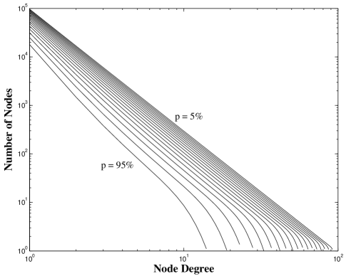
Figure 1: The degree distribution of the remaining graph when a fraction $p=5\%$–$95\%$ of the nodes in a PLN have failed, for $\beta=2.5$ and $\alpha$ chosen such that the maximum degree was $130$. The graph follows a rough power law with an increase in slope and a growing rolloff.

Our initial numerical and experimental work indicated that when $G$ is a PLN, the number of surviving nodes in $G^{\prime}$ of degree $k\geq 1$ follow an approximate power-law degree distribution (Figure 1). In finite networks, these surviving distributions will exhibit a rolloff. The observed rolloffs in these distributions make the graph less robust—the rolloff is comparable to targeted attacks, which cause SFNs to collapse more quickly (cohen01breakdown, ; dorogovtsev01comment, ). Also, the low-degree behavior of the surviving graph remains very consistent, suggesting the critical slope will not be affected (low-degree behavior such as raising the minimum degree etc. can dramatically increase $\beta_{0}$ or eliminate the critical slope entirely). Using a power law approximation with no rolloff and comparing the slope to the same critical $\beta_{0}$ should thus give us a reasonable bound on robustness to random failures.

The number of nodes $|G|$ in a PLN with $\beta>1$ is approximately $\zeta(\beta)e^{\alpha}$ (aiello00random, ), using the Riemann Zeta function $\zeta(t)=\Sigma_{n=1}^{\infty}\frac{1}{n^{t}}$. This gives the expected number of nodes of degree $k\geq 1$ in $G$ and $G^{\prime}$. For $G^{\prime}$ we will also account for orphaned nodes (nodes which have not failed but whose neighbors have all failed, leaving them with degree $0$). For us this is crucial—orphans should not be considered faulty, as they are only isolated members of the subpopulation of interest.

Assuming $G^{\prime}$ is suitably approximated with a power-law, it remains to derive the parameters of $G^{\prime}$ and determine from $\beta$ and $p$ when $\beta^{\prime}<\beta_{0}$. If failures occur with failure probability $p$ in a graph with degree distribution $c(G,k)=e^{\alpha}k^{-\beta}$ the new degree distribution (tightly bounded around its expectation) will be

$$c(G^{\prime},k)=(1-p)\sum_{k_{0}=k}^{e^{\frac{\alpha}{\beta}}}\frac{e^{\alpha}}{k_{0}^{\beta}}{k_{0}\choose k}(1-p)^{k}p^{k_{0}-k}\mbox{.}$$

Which for degree $0$ and $1$ reduce to

$$c(G^{\prime},0)=(1-p)e^{\alpha}\chi\mbox{,}\quad \chi\stackrel{{\scriptstyle\mbox{\tiny def}}}{{=}}\sum_{k_{0}=1}^{e^{\frac{\alpha}{\beta}}}\frac{1}{k_{0}^{\beta}}p^{k_{0}}\mbox{, and}$$

$$c(G^{\prime},1)=(1-p)e^{\alpha}\xi\mbox{,}\quad \xi\stackrel{{\scriptstyle\mbox{\tiny def}}}{{=}}\sum_{k_{0}=1}^{e^{\frac{\alpha}{\beta}}}\frac{1}{k_{0}^{\beta}}k_{0}(1-p)p^{k_{0}-1}$$

(noting the definitions of $\chi$ and $\xi$). Estimating the new distribution with a power law $c(G^{\prime},k)\approx e^{\alpha^{\prime}}k^{-\beta^{\prime}}$ gives $c(G^{\prime},1)\approx e^{\alpha^{\prime}}=(1-p)e^{\alpha}\xi$ and we directly obtain $\alpha^{\prime}=\alpha+\ln((1-p)\xi)$. To find $\beta^{\prime}$, note that of the original $|G|$ nodes there are an expected $p|G|$ failed nodes, $c(G^{\prime},0)$ orphaned nodes, and $|G^{\prime}|$ nodes captured by the size estimate of the new graph given the new parameters. For $\beta>1$,

$$|G| = p|G|+|G^{\prime}|+c(G^{\prime},0)$$

$$\zeta(\beta)e^{\alpha} = p\zeta(\beta)e^{\alpha}+\zeta(\beta^{\prime})e^{\alpha^{\prime}}+(1-p)e^{\alpha}\chi$$

$$\zeta(\beta)e^{\alpha} = p\zeta(\beta)e^{\alpha}+\zeta(\beta^{\prime})(1-p)e^{\alpha}\xi+(1-p)e^{\alpha}\chi$$

and solving for $\beta^{\prime}$ gives

$$(1-p)\zeta(\beta)e^{\alpha} = \zeta(\beta^{\prime})(1-p)e^{\alpha}\xi+(1-p)e^{\alpha}\chi$$

$$\zeta(\beta) = \zeta(\beta^{\prime})\xi+\chi$$

$$\beta^{\prime} = \zeta^{-1}\left(\frac{\zeta(\beta)-\chi}{\xi}\right)\mbox{.}$$

Numerical estimation shows that $\beta^{\prime}>\beta$, and this difference varies with $p$. Figures 2 and 3 show that for $\beta>2$ there are critical failure rates $p_{c}$ for which $\beta^{\prime}=\beta_{0}$, beyond which the surviving graph will not have a giant component. This shows that power-law networks are not generally robust to random node failures. However, our result depends upon a potentially coarse approximation and (although we have noted this approximation should certainly result in an upper bound on $p_{c}$) we would like an indication of how accurate our bounds are, and some validation of our methodology. The next section will present additional evidence gathered by observing failures in simulated graphs.

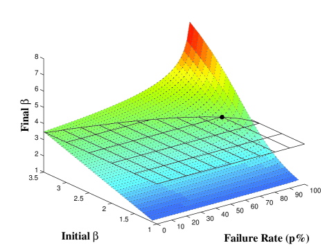
Figure 2: The function $\beta^{\prime}(\beta,p)$ for $1.1\leq\beta\leq 3.5$ and $0\leq p\leq 99\%$. For $\beta^{\prime}\geq\beta_{0}$ (intersecting plane), no giant component exists in $G^{\prime}$. An Internet-like PLN with $\beta=2.5$ will cease to have a giant component when $p=89.8\%$ (point emphasized).

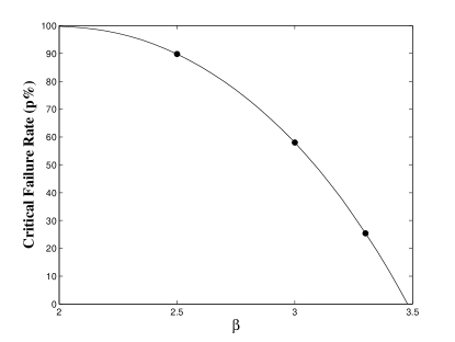
Figure 3: The critical failure rate $p$ for which $\beta^{\prime}(\beta,p)=\beta_{0}$, for $2<\beta<\beta_{0}$. The critical points for the curves of $\beta=2.5$ ($p=89.8\%$), $3.0$ ($p=58.0\%$), and $3.3$ ($p=25.4\%$) are emphasized for their correspondence with empirically studied real networks (csanyi04structure, ; reed04brief, ; saroiu02measurement, ).

4 Simulation Methods and Results

Using $c(G,k)=e^{\alpha}k^{-\beta}$ we generated node-degree histograms matching a power law, and recorded ($\beta$, $\alpha$) pairs that produced histograms averaging one million nodes. The histograms were used to populate an array of vertex-numbered “edge stubs,” the stubs were permuted randomly to create a random configuration (bollobas85random, ), and pairs of stubs were added as edges in a multigraph.

The random configuration produces multigraphs which match a node degree distribution, but it is reasonable to wonder if redundant arcs and self-arcs are frequent enough to conflict with the assumptions of independence implicit in our derivations. From (aiello00random, ) we estimated their likelihood given the number of edges in the graph and the highest expected degree, and established that they are infrequent. For $\beta>2$ the likelihood of an individual edge of the highest-degree node being a self-arc is $2/\zeta(\beta-1)e^{\frac{\beta-1}{\beta}\alpha}$, which approaches zero in large PLNs.

We used an iterated 3-coloring algorithm to identify the giant and secondary components in $G$. To simulate failures, nodes were pre-colored with probability $p$ and the algorithm run again to collect the components of $G^{\prime}$. For each $\beta$ and $p$ twenty independent graphs were created, with mean and standard deviations collected for several statistics.

For $2\leq\beta\leq 3.5$ and $0\leq p\leq 0.99$ we computed the size of the first and second largest components, the number of surviving nodes outside the largest component, and the number of orphans. The range was chosen to include $2$, a transition point of interest in regards to the density of edges in a PLN (aiello00random, ), and $3.5$, to demonstrate random failures in a graph with no giant component. For $\beta=2.5$ the data can be seen in Figure 4.

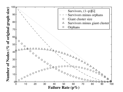
Figure 4: Simulation results for $\beta=2.5$, and $\alpha$ chosen such that $n\approx 10^{6}$. Initial giant component size and critical failure rate vary with $\beta$ but this behavior is representative of $2<\beta<\beta_{0}$. Note the decreasing fractional size of the giant component $\Circle$, and the increasing population of orphans $\square$ and nodes in small components in general $\vartriangle$.

For those familiar with the literature, the initial size of the giant component in Figure 4 may come as a surprise. For $\beta<2$ the fraction of the graph in the giant component is indirectly given in (aiello01random, ) and it is known to comprise virtually the entire graph. The probability that a random PLN node is in the giant component is approximately $1-\frac{2\log\alpha}{\alpha}$ for $\beta=2$ and approximately $1-\Theta\left(\mbox{exp}[{-\frac{(2-\beta)}{(3-\beta)\beta}\alpha}]\right)$ for $\beta<2$, both of which approach $1$ in the limit. For $2<\beta<\beta_{0}$ no such equation has been published, but in simulations the fractional size of the giant component decreases prior to its complete dissolution at $\beta_{0}$ as shown in Figure 5, subject to some scale effects. We have not seen this published elsewhere and the result was somewhat unexpected, so we include it here.

Figure 5: The fraction of nodes in the giant component (in simulation) for $2\leq\beta<\beta_{0}$, when $n\approx 10^{6}$. These numbers varied with $\alpha$; for $\beta=2$ the fraction of nodes in the giant component approaches $1$ in the limit (aiello01random, ), but for practical purposes (and possibly in the limit) the giant component for $\beta>2$ can be a small fraction of the graph.

Figure 6 presents the central result of our simulations against our mathematical predictions. The solid lines depict $|G^{\prime}|/|G|$ (i.e. $(1-p)\zeta(\beta^{\prime})e^{\alpha}\xi/\zeta(\beta)e^{\alpha}$ for select values of $\beta$—the difference between these curves and the ideal (the diagonal, $(1-p)|G|$) is the number of orphaned nodes. These curves are terminated and vertical lines are drawn at the point when $\beta^{\prime}=\beta_{0}$. Over these curves are plotted pointwise observations of these quantities in simulations of networks with $10^{6}$ nodes. The match is virtually exact, as one might expect—the combinatorics of the predictions is simply being exercised stochastically in the simulation. Finally and most importantly, Figure 6 plots the decreasing size of the giant component in the graph for comparison with the vertically distinguished critical failure rates. In this case the simulation is being compared to our approximation, and we see that the giant component falls away to virtually nothing as the failure rate approaches the predicted critical point.

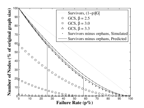
Figure 6: Predicted and actual unorphaned survivors, predicted critical failure rates, and giant component size, for $\beta=2.0$, $2.5$, $3.0$, and $3.3$, as a function of $p$. The predicted number of unorphaned survivors, $(1-p)\zeta(\beta^{\prime})e^{\alpha}\xi/\zeta(\beta)e^{\alpha}$, closely matches observed unorphaned survivors (as expected of a tightly bounded combinatorial result). More importantly, the giant component sizes ($\Circle$ $\square$ $\vartriangle$) fall away close to the predicted critical failure rates (vertical drop). Giant component sizes for $\beta=3.0$ and $3.3$ are truncated for clarity at 75% and 50%, respectively.

We conclude with a graph emphasizing the decay of the giant component itself, Figure 7. While $\beta^{\prime}<\beta_{0}$ some constant-order (although potentially small) fraction of the edge-bearing nodes in $G^{\prime}$ will almost surely remain in a giant component. Let $m$ be the size of the giant component in $G$ and $m^{\prime}$ its size in $G^{\prime}$. Then ideally $m^{\prime}=(1-p)m$, but this is clearly not the case. This graph also magnifies the disintegration of the giant component shown in Figure 6, particularly in the extreme case of $\beta=3.3$. In this case, the giant component is a small (but constant-order) fraction of the graph to begin with, and as the graph decays it is subject to greater uncertainty in its fate (this curve was the only one with a substantive standard deviation), so that it is not clear that it decays. For this case, we include the average size of the second largest component $\phi$, divided by $m$ (this value is graphically indistinguishable from zero in the other three cases). Through comparison of $m^{\prime}/m$ with $\phi/m$ it appears that the giant component has lost its status by the predicted critical point.

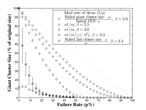
Figure 7: The ratio of the size of the giant component remaining after failure to its size before failure, for $\beta=2.0$, $2.5$, $3.0$, and $3.3$. For $\beta=3.3$ the standard deviation is shown. For $\beta=3.3$ the giant component is a fairly small fraction of the graph, and the giant component’s disintegration is shown by observing the fractional size of the second largest component falls within this range by the predicted critical failure rate of $25.4\%$. For $\beta=3.0$ and $3.3$ the plots are truncated for clarity at $75\%$ and $50\%$, respectively.

5 Conclusions and Future Work

It is probably clear to any network administrator that static graph theory has little to say about the resilience of the Internet to random failures over time: the Internet is a massive computer network with people responsible for repairing faults as they occur. Nevertheless, the random simultaneous failure model is appropriate when reasoning about the connectivity of randomly distributed subpopulations in the network. We believe we have shed some light on the subtleties of a result that has been applied too generally. By explicitly considering orphans in the failure process of a PLN, and considering graphs of minimum degree $1$, we have refined the Internet resilience result of (cohen00resilience, ) for finite networks. Thus we have better estimated when such a network would completely disintegrate as a function of its initial slope parameter and failure rate. In particular we have what we believe to be a more accurate critical failure rate for the Internet, and we show that this is not as resilient as originally suggested.

Because we are citing it so extensively, it is worth stating two additional observations in (cohen00resilience, ), to avoid confusion. Cohen et al. make casual reference to the breakdown of the SFN giant component under moderate failure levels when $\beta=3.5$. Although reasonable in general, in pure power-law networks there is no giant component when $\beta>\beta_{0}=3.47875$ (aiello00random, ). Also confusing may be their graph of the fractional size of the giant component remaining as a function of the failure rate $p$, when $\beta=2.5$ (a graph analogous to our Figure 7). This ratio is graphed in such a way that it appears to very closely follow, and even exceed, $(1-p)n$—in other words, the surviving component’s size appears to exceed the expected number of survivors. In fact the figure graphs this quantity divided by $(1-p)$, and thus in fact matches our results in Figure 7 for the values of $\beta$ they present ($2.5$ and $3.5$). This graph has been reproduced in several places without elaboration albert02statistical .

We have analytically considered these matters for finite PLNs under the full range $0<\beta<\beta_{0}$, but have not yet confirmed our results in simulation for $\beta<2$. Observing how our results vary for networks over several orders of magnitude larger and smaller also remains to be done. Doing so will require a more substantial simulation than we have implemented. Beyond pure power-law degree distributions, a more general class of PLNs with rolloff and offset terms should also be studied. In particular, most real world networks that approximate a power law exhibit a rolloff. Finally, for $2<\beta<\beta_{0}$ we have been unable to find a derivation of the fractional size of the giant component of the graph in the limit, and such a formula would be of interest. Extending the model to consider assortative networks, conditional failure models, and other variations that affect the critical failure threshold could lead to a number of interesting new results.

6 Acknowledgements

We would like to thank Dr. Reuven Cohen for his review and comments of the manuscript, and would also like to thank both Dr. Cohen and Dr. Lu for their responses to our questions.

References

- (1) R. Cohen, K. Erez, D. ben Avraham, S. Havlin, Resilience of the Internet to random breakdowns, Physical Review Letters 85 (21).
- (2) W. Aiello, F. Chung, L. Lu, A random graph model for massive graphs, in: STOC, Portland, OR, 2000, pp. 171–180.
- (3) R. Albert, A.-L. Barabási, Statistical mechanics of complex networks, Rev. Mod. Phys. 74 (2002) 47–98.
- (4) M. Faloutsos, P. Faloutsos, C. Faloutsos, On power-law relationships of the internet topology, in: SIGCOMM ’99: Proceedings of the conference on Applications, technologies, architectures, and protocols for computer communication, ACM Press, New York, NY, USA, 1999, pp. 251–262.
- (5) H. Chang, R. Govindan, S. Jamin, S. Shenker, W. Willinger, Towards capturing representative AS-level Internet topologies, Computer Networks Journal 44 (6) (2004) 737–755.
- (6) G. Csányi, B. Szendrői, Structure of a large social network, Physical Review 69 (036131).
- (7) W. J. Reed, A brief introduction to scale-free networks, unpublished work found at http://www.math.uvic.ca/faculty/reed/draft_1.pdf at the Department of Mathematics and Statistics, University of Victoria (May 18 2004).
- (8) S. Saroiu, P. K. Gummadi, S. D. Gribble, A measurement study of peer-to-peer file sharing systems, in: Proceedings of the Multimedia Computing and Networking (MMCN), San Jose, CA, 2002, pp. 156–170.
- (9) H. Link, J. Saia, T. Lane, R. Laviolette, The impact of social networks on multi-agent recommender systems, in: Proceedings of the Workshop on Cooperative Multi-Agent Learning (PKDD ’05), Porto, Portugal, 2005.
- (10) M. E. J. Newman, Mixing patterns in networks, Physical Review E 67 (026126).
- (11) M. Molloy, B. Reed, A critical point for random graphs with a given degree sequence, Random Structures and Algorithms 6 (1995) 161–180.
- (12) M. Molloy, B. Reed, The size of the giant component of a random graph with a given degree sequence, Combinatorics, Probability and Computing 7 (1998) 295–305.
- (13) R. Otter, The number of trees, Annals of Mathematics 49 (3) (1948) 583–599.
- (14) R. Otter, The multiplicative process, Annals of Mathematical Statistics 20 (2) (1949) 206–224.
- (15) B. Mohar, The laplacian spectrum of graphs, in: Y. Alavi, G. Chartrand, O. Oellermann, A. Schwenk (Eds.), Graph Theory, Combinatorics and Applications, Vol. 2, Wiley, New York, 1991, pp. 871–898.
- (16) D. Achlioptas, A. Clauset, D. Kempe, C. Moore, On the bias of traceroute sampling, or: Why almost every network looks like it has a power law, in: Proceedings of the 2005 Symposium on the Theory of Computation (STOC), Baltimore, MD, 2005, pp. 694–703.
- (17) B. Awerbuch, B. Patt-Shamir, D. Peleg, M. Tuttle, Improved recommendation systems, in: Proceedings of the Sixteenth Annual ACM-SIAM Symposium on Discrete Algorithms (SODA ’05), SIAM, ACM, Vancouver, BC, CA, 2005.
- (18) D. Kempe, J. Kleinberg, É. Tardos, Maximizing the spread of influence in a social network, in: Proceedings of KDD 2003, Washington, DC, 2003.
- (19) D. J. Watts, S. H. Strogatz, Collective dynamics of ’small-world’ networks, Nature 393 (1998) 440–442.
- (20) S. N. Dorogovtsev, J. F. F. Mendes, The shortest path to complex networks, arXiv:cond-mat/0404593 v1 (April 24 2004).
- (21) W. Aiello, F. Chung, L. Lu, A random graph model for power law graphs, Experimental Mathematics 10 (1) (2001) 53–66.
- (22) R. Cohen, K. Erez, D. ben Avraham, S. Havlin, Breakdown of the Internet under intentional attack, Physical Review Letters 86 (16).
- (23) S. N. Dorogovtsev, J. F. F. Mendes, Comment on ‘Resilience of the Internet to Random Breakdowns’, Physical Review Letters 87.
- (24) B. Bollobás, Random Graphs, Academic Press, London, UK, 1985.
- (25) W. Aiello, L. Lu, email with authors, confirming typographical errors in ‘A random graph model for power law graphs,’ in Experimental Mathematics (May 2005).
- (26) R. Cohen, email with author, confirming typographical errors in ‘Resilience of the Internet to random breakdowns,’ in Phys. Rev. Lett. (September 2005).