A simple effective method for curvatures estimation on triangular meshes

Abstract

To definite and compute differential invariants, like curvatures, for triangular meshes (or polyhedral surfaces) is a key problem in CAGD and the computer vision. The Gaussian curvature and the mean curvature are determined by the differential of the Gauss map of the underlying surface. The Gauss map assigns to each point in the surface the unit normal vector of the tangent plane to the surface at this point. We follow the ideas developed in Chen and Wu [2](2004) and Wu, Chen and Chi[11](2005) to describe a new and simple approach to estimate the differential of the Gauss map and curvatures from the viewpoint of the gradient and the centroid weights. This will give us a much better estimation of curvatures than Taubin’s algorithm [10] (1995).

Jyh-Yang Wu Sheng-Gwo Chen, and Mei-Hsiu Chi

1 Introduction

The tensors of curvatures on a regular surface $\Sigma$ in the 3D Euclidean space are important differential invariants in the theory of surfaces and its applications. Gaussian curvatures and mean curvatures are determined by the differential of the Gauss map on the surface $\Sigma$. Given a basis on the tangent plane of a point p on the surface $\Sigma$, the differential $dN$ of the Gauss map $N$ can be realized as a $2\times 2$ symmetric matrix $A$. In fact, the Gaussian curvature and the mean curvature at the point $p$ can be computed from the determinant and the trace of the matrix $A$. Since 1990, many methods, like Chen and Schmitt [1](1992) and Taubin [10] (1995), to estimate these curvatures are proposed. However, most of them are devoted to the investigation of the principal curvatures, but not directly from the differential of the Gauss map. Usually, the accurate estimation of curvatures at vertices on a triangular mesh plays as the first step for many applications such as simplification, smoothing, subdivision, visualization and registration, etc.

Chen and Schmitt [1] (1992) and Taubin [10](1995) employed the circular arcs to approximate the normal curvatures. Their methods need to estimate the Euler formula and may cause large errors. In this note, we follow the methods developed by Chen and Wu [2, 3](2004, 2005) and Wu, Chen and Chi [11](2005) to estimate the differential $dN$ of the Gauss map directly and then obtain accurate estimations of the Gaussian curvature and the mean curvature. This method follows the line of the differential of the Gauss map more directly and thus provides us a conceptually simple algorithm to estimate curvatures on a triangular mesh. Since our method is more natural, the estimation turns out to be more accurate. Indeed, it performs much better than many other proposed methods. In section two we recall the basic theory about the differential of Gauss map on a regular surface. In section three, we briefly review the methods of Chen and Schmitt, and Taubin to estimate curvatures on triangular meshes. In section four, we present our method for estimating the differential of the Gauss map and curvatures on a triangular mesh. In section five, we compare the results of our method with Taubin’s method.

2 The Gauss map and curvatures on regular surfaces

Consider a parameterization $x:U\rightarrow\Sigma$ of a regular surface $\Sigma$ at a point $p$, where $U$ is an open subset of the 2D Euclidean space $\mathbb{R}^{2}$. We can choose, at each point $q$ of $x(U)$, an unit normal vector $N(q)$. The map $N:x(U)\rightarrow S^{2}$ is the local Gauss map from an open subset of the regular surface $\Sigma$ to the unit sphere $S^{2}$ in the 3D Euclidean space $\mathbb{R}^{3}$. The Gauss map $N$ is differentiable and its differential $dN$ of $N$ at $p$ in $\Sigma$ is a linear map from the tangent space into itself.

Given an orthogonal basis $\{e_{1},e_{2}\}$ for the tangent space $T\Sigma_{p}$, we can find a $2\times 2$ matrix $A$ to represent the Gauss map as follows: set $a_{ij}$ to be the inner product of the vector $e_{i}$ with $dN_{p}(e_{j})$. That is,

$$a_{ij}=<e_{i},dN_{p}(e_{j})>.$$ (1)

Thus the matrix $A=(a_{ij})$ represents the linear map $dN_{p}$. Given a vector $v=\alpha_{1}e_{1}+\alpha_{2}e_{2}$ in $T\Sigma_{p}$, $dN_{p}(v)$ is equal to $w=\beta_{1}e_{1}+\beta_{2}e_{2}$ where $\beta_{1}$ and $\beta_{2}$ satisfy

$$\begin{pmatrix}\beta_{1}\cr\beta_{2}\end{pmatrix}=\begin{pmatrix}a_{11}&a_{12}\cr a_{21}&a_{22}\end{pmatrix}\begin{pmatrix}\alpha_{1}\cr\alpha_{2}\end{pmatrix}$$ (2)

Under this representation of the linear map $dN_{p}$, the Gaussian curvature $K$ and the mean curvature $H$ can be computed by $K=\det(A)$ and $H=-\frac{\mbox{ trace}(A)}{2}$. Namely,

$$K=a_{11}a_{22}-a_{12}a_{21}$$ (3)

$$H=-\frac{a_{11}+a_{22}}{2}$$ (4)

Indeed, since the linear map $dN_{p}$ is self-adjoint, the matrix $A$ should be symmetric and diagonalizable. Its eigenvalues are $-\kappa_{1}$ and $-\kappa_{2}$. The values $\kappa_{1}$ and $\kappa_{2}$ are the principal curvatures and their associated eigenvectors $v_{1}$ and $v_{2}$ are called the principal directions. In terms of the principal curvatures $\kappa_{1}$ and $\kappa_{2}$, we have the Gaussian curvature $K=\kappa_{1}\kappa_{2}$ and the mean curvature $H=\frac{\kappa_{1}+\kappa_{2}}{2}$.

Consider a regular curve $c(s)$ with arc length in the regular surface $\Sigma$ and $c(0)=p$. The number $k_{n}=<c^{\prime\prime}(0),N(p)>$ is called the normal curvature of $c(s)$ at $p$. Meusnier’s Theorem [4](1976) implies that all curves at $p$ with the same tangent vector will have the same normal curvature. This allows us to speak of the normal curvature along a unit tangent vector at $p$. The maximum and the minimum normal curvatures are nothing but the principal curvatures $\kappa_{1}$ and $\kappa_{2}$. Moreover, we have, for any unit vector $v$ in $T\Sigma_{p}$,

$$v=v_{1}\cos\theta+v_{2}\sin\theta$$ (5)

where $v_{1}$ and $v_{2}$ are the principal directions and $\theta$ is the angle between the vectors $v$ and $v_{1}$. The normal curvature $k_{n}$ along the unit vector $v$ is given by

$$k_{n}(v)=\kappa_{1}\cos^{2}\theta+\kappa_{2}\sin^{2}\theta$$ (6)

This is known as the Euler formula.

3 The normal curvature approach: Chen and Schmitt’s method and Taubin’s method

In this section we shall review the methods given by Chen and Schmitt [1](1992) and Taubin [10](1995). First we introduce some notations. Consider a triangular mesh $S=(V,F)$, where $V=\{v_{i}|1\leq i\leq n_{v}\}$ is the list of vertices and $F=\{f_{k}|1\leq k\leq n_{F}\}$ is the list of triangles. We assume $S$ is oriented and consistent. That is, neighboring triangles have the normals pointing to the same side of the surface. For a given vertex $v$ in $V$, we say that another vertex $w$ is a neighbor vertex of $v$ if there is a triangle $f$ in $F$ such that $v$ and $w$ are both in $f$. We denote by $Ng(v)$ the set of neighbor vertices $w$ of $v$ in $V$ and $m$ the number of points in $Ng(v)$. We also denote by $T(v)$ the set of triangles $f$ in $F$ with $v\in f$. If the triangle $f$ is in $T(v)$, we say that $f$ is incident to $v$. The area of a triangle $f$ is denoted by $|f|$.

3.1 The least square method of Chen and Schmitt

Chen and Schmitt [1](1992) provided an algorithm to estimate the principal curvatures by the Euler formula. Their main idea is to choose a suitable coordinate system $\{r_{1},r_{2}\}$ on the tangent space. Given a unit vector t in the tangent plane, the Euler formula (6) will give

$$k_{n}(t)=\kappa_{1}\cos^{2}(\theta+\theta_{0})+\kappa_{2}\sin^{2}(\theta+\theta_{0})$$ (7)

where $\theta_{0}$ is the angle between the principal direction $e_{1}$ and $r_{1}$ and $\theta$ is now the angle between the unit vector $t$ and $r_{1}$. This equation (7) can be rewritten as

$$k_{n}(t)=C_{1}\cos^{2}\theta+C_{2}\cos^{2}\theta+C_{3}\cos^{2}\theta$$ (8)

for some constant $C_{1}$, $C_{2}$ and $C_{3}$.

Given a vertex $v_{i}$ in $Ng(v)$, we can obtain an unit vector $t_{i}$ in the tangent plane of $S$ at the vertex $v$ by

$$t_{i}=\frac{(v_{i}-v)-<v_{i}-v,N>N}{||(v_{i}-v)-<v_{i}-v,N>N||}$$ (9)

where $N$ is the normal vector at $v$. The normal curvature $k_{n}(t)$ along the unit vector $t_{i}$ can now be approximated by

$$k_{n}(t_{i})=\frac{2<v_{j}-v,N>}{||v-v_{i}||^{2}}.$$ (10)

See Chen and Wu [2](2004) for the discussions. Chen and Schmitt used the least square method to find the constants $C_{1}$, $C_{2}$ and $C_{3}$:

$$\min\sum_{i}\left|(C_{1}\cos^{2}\theta_{i}+C_{2}\cos\theta_{i}\sin\theta_{i}+C_{3}\sin^{2}\theta_{i})-k_{n}(t_{i})\right|^{2}$$ (11)

where $\theta_{i}$ is the angle between $t_{i}$ and $r_{1}$. The principal curvatures can then be solved from the constants $C_{1}$, $C_{2}$ and $C_{3}$ via the following relations:

$$\left\{\begin{array}[]{ll}\kappa_{1}\cos^{2}\theta_{0}+\kappa_{2}\sin^{2}\theta_{0}&=C_{1}\cr 2(\kappa_{1}-\kappa_{2})\cos\theta_{0}\sin\theta_{0}&=C_{2}\cr\kappa_{2}\cos^{2}\theta_{0}+\kappa_{1}\sin^{2}\theta_{0}&=C_{3}\end{array}\right.$$ (12)

Moreover, the principal directions can also be computed from

$$\left\{\begin{array}[]{ll}v_{1}&=\cos(-\theta_{0})r_{1}+\sin(-\theta_{0})r_{2}\cr v_{2}&=\sin(-\theta_{0})r_{1}+\cos(-\theta_{0})r_{2}\end{array}\right.$$ (13)

3.2 The integral method of Taubin

To find the principal curvatures $\kappa_{1}$ and $\kappa_{2}$, Taubin [10](1995) considered the following integral of a symmetric $3\times 3$ matrix:

$$B=\frac{1}{2}\int_{-\pi}^{\pi}k_{n}(v)vv^{T}d\theta$$ (14)

where $v=v_{1}\cos\theta+v_{2}\sin\theta$. Taubin showed that the matrix $B$ can be decomposed into

$$B=E^{T}\begin{pmatrix}m_{1}&0\cr 0&m_{2}\end{pmatrix}E$$ (15)

where $E=\begin{pmatrix}v_{1}&v_{2}\end{pmatrix}$ is the $3\times 2$ matrix given by the principal directions. Moreover, the principal curvatures are given by the relations:

$$\left\{\begin{array}[]{ll}\kappa_{1}&=3m_{1}-m_{2}\cr\kappa_{2}&=3m_{2}-m_{1}\end{array}\right.$$ (16)

Taubin approximated the integral (14) by the finite sum

$$\tilde{B}=\sum_{i=1}^{m}\omega_{i}k_{n}(t_{i})t_{i}t_{i}^{T},$$ (17)

where the unit tangent vector $t_{i}$ is given in (9) and the normal curvature is approximated as in equation (10). The weight $\omega_{i}$ is chosen to be proportional to the sum of the areas of the triangles incident to both $v$ and $v_{i}$ with $\sum_{i=1}^{m}\omega_{i}=1$. Taubin decomposed the matrix $\tilde{B}$ with a suitable transformation and a rotation. In (Chen and Wu [2]), the centroid weights were used for Equation (17) and they gave more accurate results.

3.3 Related works

Flynn and Jain [5](1989) used a suitable sphere passing through four vertices to estimate curvatures. Meek and Walton [7](2000) examined several methods and compared them with the discretization and interpolation method. Gatzke and Grim[6](2003) systematically analyzed the results of computation of curvatures of surfaces represented by triangular meshes and recommended the surface fitting methods. See also Petitjean [9](2002) for the surface fitting methods. Meyer et al.[8](2003) employed the Gauss-Bonnet theorem to estimate the Gaussian curvatures and introduced the Laplace-Beltrami operator to approximate the mean curvature.

4 The differential approach: our method

In this section we shall describe a new, simple and effective method to approximate the differential of the Gauss map. In order to simplify the presentation, we shall follow the ideas developed in Wu, Chen and Chi[3](2005) about the gradient and the Laplacian of a function defined on a triangular mesh.

Consider a triangular mesh $S=(V,F)$, where $V=\{v_{i}|1\leq i\leq n_{v}\}$ is the list of vertices and $F=\{f_{k}|1\leq i\leq n_{F}\}$ is the list of triangles. Let $g$ be a function on $V$. First, we can extend the function $g$ to a piecewise linear function, still denoted by $g$, on $S$ as follows. Given a face $f$ in $F$ with vertices $v_{i}$, $v_{j}$ and $v_{k}$, every point $p$ in $f$ can be written as an unique linear combination of $v_{i}$, $v_{j}$ and $v_{k}$. That is, $p=\alpha v_{i}+\beta v_{j}+\gamma v_{k}$ with $\alpha,\beta,\gamma\geq 0$ and $\alpha+\beta+\gamma=1$. Then we define $g(p)$ by

$$g(p)=\alpha g(v_{i})+\beta g(v_{j})+\gamma g(v_{k})$$ (18)

Thus, the function $g$ is affine on each face $f$ of $S$ and hence is differentiable on $f$. The gradient $(\nabla g)_{f}$ of $g$ on the face $f$ at the vertex $v_{i}$ can be computed from

$$(\nabla g)_{f}(v_{i})=a(v_{j}-v_{i})+b(v_{k}-v_{i})$$ (19)

where the coefficients $a$ and $b$ are determined by the relations

$$\begin{array}[]{ll}g(v_{j})-g(v_{i})&=<(\nabla g)_{f}(v_{i}),v_{j}-v_{i}>,\cr g(v_{k})-g(v_{i})&=<(\nabla g)_{f}(v_{i}),v_{k}-v_{i}>,\cr\end{array}$$ (20)

A direct computation gives

$$\begin{pmatrix}a\cr b\end{pmatrix}=\begin{pmatrix}<v_{j}-v_{i},v_{j}-v_{i}>,&<v_{j}-v_{i},v_{k}-v_{i}>\cr<v_{j}-v_{i},v_{k}-v_{i}>,&<v_{k}-v_{i},v_{k}-v_{i}>\end{pmatrix}^{-1}\begin{pmatrix}g(v_{j})-g(v_{i})\cr g(v_{k})-g(v_{i})\end{pmatrix}$$ (21)

To obtain the gradient $\nabla g(v_{i})$ of $g$ on $S$ at the vertex $v_{i}$, we use the weighted combination method. Namely, we set

$$\nabla g(v_{i})=\sum_{f\in T(v_{i})}\omega_{f}[(\nabla g)_{f}(v_{i})]$$ (22)

with $\omega_{f}\geq 0$ and $\sum_{f\in T(v_{i})}\omega_{f}=1$. According to Chen and Wu [2, 3](2004, 2005), we shall use the centroid weight for the gradient formula (22). The centroid weights are

$$\omega_{f}=\frac{\frac{1}{||G_{f}-v_{i}||^{2}}}{\sum_{f\in T(v_{i})}\frac{1}{||G_{f}-v_{i}||^{2}}}$$ (23)

where the centroid $G_{k}$ of the triangle face $f$ is determined by

$$G_{f}=\frac{v_{i}+v_{j}+v_{k}}{3}$$ (24)

Next we consider the differential $dN$ of the Gauss map $N$. As in Chen and Wu[2](2004), we define the normal vector $N(v)$ at each vertex $v$ in $V$ by the centroid weights:

$$N(v)=\frac{\sum_{f\in T(v)}\omega_{f}N_{f}}{\left\|\sum_{f\in T(v)}\omega_{f}N_{f}\right\|}$$ (25)

where $N_{f}$ is the unit normal to the triangle face $f$ and the weight $\omega_{f}$ is given in (23). The normal vector $N(v)$ has three components:

$$N(v)=\begin{pmatrix}n_{1}(v),n_{2}(v),n_{3}(v)\end{pmatrix}^{T}$$ (26)

and its components $n_{i}(v)$ are functions on $V$. Thus, we can compute their gradients and obtain the differential $dN_{v}$ of $N$ at the vertex $v$ as

$$dN_{v}=\begin{pmatrix}\nabla n_{1}(v),\nabla n_{2}(v),\nabla n_{3}(v)\end{pmatrix}.$$ (27)

Note that the differential $dN_{v}$ is a $3\times 3$ matrix. In order to obtain the linear map $dN_{v}$ from the tangent space $TS_{v}$ into itself, we choose an orthonormal basis $\{e_{1},e_{2}\}$ for the tangent space $T\Sigma_{p}$. That is, the vectors $e_{1}$, $e_{2}$ and $N(v)$ form an 3-dimensional orthonormal basis. Then the differential $dN_{v}$ can be realized by a $2\times 2$ matrix, still denoted by $dN_{v}=\begin{pmatrix}a_{ij}\end{pmatrix}$, and the entry $a_{ij}$ is given by

$$a_{ij}=<e_{i},dN_{v}(e_{j})>.$$ (28)

Therefore, we can estimate the Gaussian curvature $K$ and the mean curvature $H$ by

$$\begin{array}[]{ll}K&=a_{11}a_{22}-a_{12}a_{21}\cr H&=-\frac{a_{11}+a_{22}}{2}\end{array}$$ (29)

The principal curvatures and the principal directions can also be computed from the eigenvalues and eigenvectors of $dN_{v}$.

5 Computational Results

Taubin’s method to estimate the tensors product of curvature on triangular mesh is very useful in CAD. Furthermore, Chen and Wu [1] (2004) provided a better choice in Taubin’s algorithm by centroid weights. We will compare Taubin’s method by centroid weights and our method. In our tests, we consider the random polynomial surface,

$$\Sigma=\{(u,v,f(u,v))\}$$ (30)

with

$$f(u,v)=\sum_{i=0}^{m}\sum_{j=0}^{n}c_{ij}u^{i}v^{j}$$

We compute the Gaussian curvature at the vertex $p=(0,0,f(0,0))$ on some different random surfaces. The set of neighbors of $p$ is constructed by

$$\{(r_{i}\cos\theta_{i},r_{i}\sin\theta_{i},f(r_{i}\cos\theta_{i},r_{i}\sin\theta_{i}))|i\in\{1,2,\cdots,n_{V}\}\}$$ (31)

In equations 30 and 31, $c_{ij}$ is a random number in the interval $[-5,5]$, $\{\theta_{0},\theta_{1},\cdots\theta_{n_{V}}\}$ is a random partition of $[0,2\pi]$ such that $0<|\theta_{j+1}-\theta_{j}|<1.9\pi$ for each $j$ and $m,n,r_{i},n_{V}\in\mathbb{R}^{+}$ are some random positive values. And we estimate the error of Gaussian curvatures by the formula

$$Err(K)=\frac{|K-K_{v}|}{K}$$

where $K$ is the real Gaussian curvature at vertex $v$ and $K_{v}$ is the Gaussian curvature at vertex $v$ obtained by Taubin’s method or our method.

From figure 1 to 3, we tests 1,000 random surfaces. For each surface, we compute the error of average of 10,000 different random partitions. From these figures, our method is better than the Taubin’s method. In Figures 4, 5 and 6, we test the effect of different partitions. For each partition, we choose 10,000 differential random surfaces and estimate the error of average and standard derivation. Obviously, Our method is more stable than the Taubin’s method.

Final Remark:
This method is conceptually simple and more natural than the normal curvature method of Chen and Schmitt and Taubin. In the next section, we shall show that this method also yields more accurate results. In Wu, Chen and Chi[11](2005), the authors also develop a differential theory for triangular meshes. The gradient, Laplace-Beltrami operators are discussed. Moreover, this method also works for boundary vertices and for polyhedron meshes.

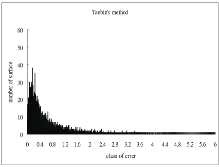
Figure 1: The effect of different surface of Taubin’s method

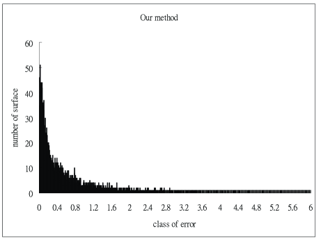
Figure 2: The effect of different surface of Our method

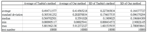
Figure 3: The table of the effect of different surface

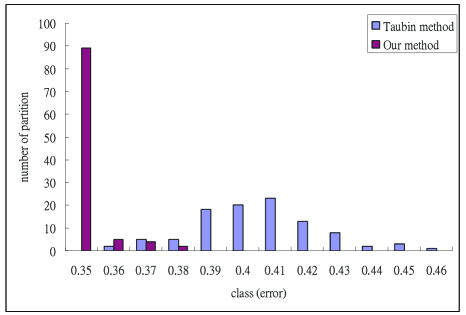
Figure 4: The effect of different partition

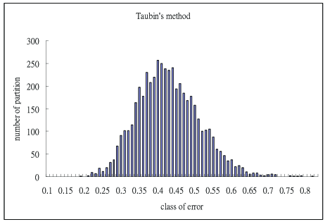
Figure 5: The effect of different partition of Taubin’s method

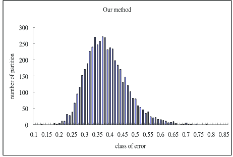
Figure 6: The effect of different partition of our method

References

- [1] Chen, X., Schmitt, F., 1992. Intrinsic Surface Properties from Surface Triangulation. Proceedings of the European Conference on Computer Vision, pp. 739-743.
- [2] Chen, S.-G., Wu, J.-Y., 2004. Estimating normal vectors and curvatures by centroid weights. Computer Aided Geometric Design, 21, pp. 447-458.
- [3] Chen, S.-G., Wu, J.-Y., 2005. A geometric interpretation of weighted normal vectors and application. Proceeding of the IEEE Computer Society Conference on Computer Graphics, Imaging and Visualization, New Trends, pp.422-425.
- [4] Do Carmo, M., 1976. Differential Geometry of curves and surfaces. Prentice Hall, Englewood Cliffs, NJ.
- [5] Flynn, P.J., Jain A.K., 1989. On reliable curvature estimation. Proceeding of the IEEE Computer Society Conference on Computer Vision and pattern Recognition, pp.110-116.
- [6] Gatzke, T., Grimm, C., 2003. Improved curvature estimation on triangular meshes. Eurographics Symposium on Geometry Processing. pp. 57-67.
- [7] Meek, D.S., Walton, D.J. 2000. On surface normal and Gaussian curvature approximations given data sampled from a smooth surface. Computer Aided Geometric Design, 17, pp. 521-543.
- [8] Meyer, M., Desbrum, M., Schroder, P., Barr, A.H., 2003. Discrete Differential Geometry Operators fot Triangulated 2-Manifolds. In: Hege, H.C., Polthier, K., (Eds), Visualization and Mathematics III. Springer Verlag, Heidelberg, Germany, pp. 35-57.
- [9] Petitjean, S., 2002. A survey of methods for recovering quagrics in triangular meshes. ACM Computing Surveys, 2(34), pp. 1-61.
- [10] Taubin, G., 1995. Estimating the tensor of curvatures of a surface from a polyhedral approximation. In: proceedings of the Fifth International Conference on Computer Vision, pp. 902-907.
- [11] Wu, J.-Y., Chen, S.-G., Chi, M-H, 2005. A simple differential theory for triangular meshes. Teachnical Report WU01, CCU. Repartment of Mathematics.