MathPSfrag: Creating Publication-Quality Labels in Mathematica Plots

Abstract

This article introduces a Mathematica^® package providing a graphics export function that automatically replaces Mathematica^® expressions in a graphic by the corresponding LaTeX constructs and positions them correctly. It thus facilitates the creation of publication-quality Enscapulated PostScript (EPS) graphics.

Introduction

Many programs producing EPS graphics do not allow the inclusion of LaTeX commands. While there exist several solutions (see for example McKay and Moore (1999)) to work around these difficulties, they all have various drawbacks. In this article, we will focus on a particular existing solution, the PSfrag package Grant and Carlisle , which provides LaTeX macros allowing to replace pieces of text (“tags”) in an EPS file by an arbitrary LaTeX construct.

However, for PSfrag to work, the application must write tags unaltered into the EPS file. For Mathematica Wolfram (1999); Wolfram Research, Inc. (2005), this requirement amounts to using single words, strictly consisting of alphanumeric characters only. As a consequence, the user has to work most of the time with an unconveniently labelled graphic and is furthermore required to keep track of the tags used in the substitution macros.

On the other hand, it is not always possible to use Mathematica’s conventional export function as it produces EPS files requiring the inclusion of additional fonts into the document, a process often not being under the author’s control. A way out is to include the font into the EPS file, or set the font family to a standard PostScript one:

Plot[…, TextStyle$\to${FontFamily$\to$"Times"}] and
Export[…, ConversionOptions$\to$
 {"IncludeSpecialFonts"$\to$True}].

(a) Conventional Mathematica plot before using MathPSfrag

\psfrag{a0A}[cr][cr][1][0]{${0}$}\psfrag{a0}[tc][tc][1][0]{${0}$}\psfrag{a1A}[cr][cr][1][0]{${1}$}\psfrag{a1}[cr][cr][1][0]{${-1}$}\psfrag{a2}[cr][cr][1][0]{${2}$}\psfrag{a2Pi}[tc][tc][1][0]{${2\pi}$}\psfrag{a3Cos2}[cr][cr][1][0]{${3\sqrt[3]{\cos^{2}\left(2\sqrt{x}\right)}}$}\psfrag{a3}[cr][cr][1][0]{${3}$}\psfrag{a3Pi2}[tc][tc][1][0]{${\frac{3\pi}{2}}$}\psfrag{localm}[tc][tc][1][0]{{{local maximum}}}\psfrag{Pi2}[tc][tc][1][0]{${\frac{\pi}{2}}$}\psfrag{Pi}[tc][tc][1][0]{${\pi}$}\psfrag{Sinx}[cl][cl][1][0]{${\sin(x)}$}\includegraphics[width=377.24727pt]{pics/ex_auto-psfrag.eps}

(b) The same plot after automatically substituting all Text primitives (including tick mark labels) by LaTeX.

Figure 1: Old vs. new graphics export mechanism.

∗ jgrosse@mppmu.mpg.de
  http://wwwth.mppmu.mpg.de/members/jgrosse

\psfrag{gA}[br][br]{---[br][br]---}\psfrag*{gA}[Br][bc][2]{---[Br][bc][2]---}\psfrag*{gA}[cr][bl]{---[cr][bl]---}\psfrag*{gA}[tr][Bl]{---[tr][Bl]---}\psfrag*{gA}[bc][Bc]{---[bc][Bc]---}\psfrag*{gA}[Bc][Br]{---[Bc][Br]---}\psfrag*{gA}[cc][cr]{---[cc][cr]---}\psfrag*{gA}[tc][cc][0.75][45]{---[tc][cc][0.75][45]---}\psfrag*{gA}[bl][cl][1.5][30]{---[bl][cl][1.5][30]---}\psfrag*{gA}[Bl][tl]{---[Bl][tl]---}\psfrag*{gA}[bl][Bl]{~{}~{}~{}~{}~{}(baseline)}\psfrag*{gA}[bl][cl]{~{}~{}~{}~{}~{}(center line)}\psfrag*{gA}[bl][tc][1][-90]{~{}~{}~{}~{}~{}(center line)}\psfrag*{gA}[cl][tc]{---[cl][tc]---}\psfrag*{gA}[tl][tr][1][180]{---[tl][tr][1][180]---}\includegraphics[width=251.50038pt]{pics/testfig.eps}

Figure 2: Illustration of the various optional arguments of the \psfrag command, taken from Grant and Carlisle with minor changes. The first option determines the alignment of the LaTeX description, while the second one is responsible for the point to which the LaTeX macro is attached.

While the slight mismatch between the PostScript font’s appearance, cf. fig. 1(a), and that of LaTeX’s standard font (Computer Modern) may be acceptable in case of ordinary text labels, mathematical expressions like square roots or fractions cannot compete with LaTeX’s typesetting quality in this approach. Consequently, some authors simply restrict labelling of Mathematica plots to a bare minimum.

MathPSfrag Große is a package that conveniently produces publication-quality labels in EPS files generated by Mathematica. MathPSfrag automates many (often all) tedious details related to the use of the standard LaTeX package PSfrag, while still allowing manual fine tuning. As a demonstration of the degree of automation, compare fig. 1(a), which has been generated by using the standard Mathematica command Export, and fig. 1(b), generated by MathPSfrag’s export instruction.

While the solution presented here, relies on the PSfrag package, it avoids many of its shortcomings by providing a semi-automatic layer. In particular,

• in most cases, it is sufficient to simply use the new PSfragExport command,

• including the graphic into the document requires only one additional command.

This article is organized as follows. A short review of PSfrag and a somewhat longer explanation of the semi-automatic features provided by MathPSfrag, are given in the first and second section, respectively. The third part contains several examples whose code as well as that of figures 1(a) and 1(b) is contained in the appendix. Finally, some of MathPSfrag’s internals are discussed.

I Review of PSfrag

This is intended to be a short introduction into PSfrag explaining only the essential features necessary to understand the corresponding Mathematica package’s internals and to take advantage of its manual options if automatic placement does not yield the desired result. The full documentation can be found in Grant and Carlisle .

PSfrag provides the macro

\psfrag$\langle$tag$\rangle$[$[$posn$]$][$[$psposn$]$][$[$scale$]$][$[$rot$]$]$\langle$LaTeX$\rangle$,

which replaces any occurence of $\langle$tag$\rangle$ in the output of an EPS file by $\langle$LaTeX$\rangle$. According to Grant and Carlisle , “all \psfrag calls that precede an \includegraphics (or equivalent) in the same or surrounding environments” will affect the output of the included graphics, i.e. \psfrag commands can be defined either locally, to act on stricly one graphic, or globally, thus acting on all graphics in a document.

$[$posn$]$ and $[$psposn$]$ are optional arguments which allow to set (first) the vertical (top, bottom, Baseline, or center) and (second) the horizontal (left, right, center) alignment of the replacement text by specifying the respective first character of the choices given in parentheses. The arguments refer to the position of the reference point in the respective bounding boxes. The LaTeX construct is placed such that its reference point is at the position of the corresponding PostScript (tag) box’ reference point, cf. fig. 2.

\psfrag{ExamplA}[cc][cc][1][0]{{{Example 90}}}\psfrag{ExamplB}[cc][cc][1][0]{{{Example 150}}}\psfrag{ExamplC}[cc][cc][1][0]{{{Example 210}}}\psfrag{Exampl}[cc][cc][1][0]{{{Example 30}}}\psfrag{ExamplD}[cc][cc][1][0]{{{Example 270}}}\psfrag{ExamplE}[cc][cc][1][0]{{{Example 330}}}\includegraphics[width=390.25534pt]{pics/ex_rot-psfrag.eps}

Figure 3: Example for substituting rotated text. To demonstrate that the new export function can preserve the orientation, only half of the labels have been substituted by LaTeX.

$[$scale$]$ and $[$rot$]$ permit scaling and rotation of the inserted box, where the rotation is relative to the slope of the PostScript bounding box such that a value of “0” preserves the orientation, see fig. 3. Scaling is best achieved by using LaTeX scaling commands, like \Large, instead of the $[$scale$]$ option, since the standard LaTeX fonts consists of bitmaps rendered specifically for the chosen size and do not rescale well. As will be demonstrated in the example section, MathPSfrag provides macro hooks that allow to scale labels retroactively from within the document.

II How to use MathPSfrag

There are only two commands needed to control MathPSfrag’s EPS generation: PSfragExport, which supersedes Mathematica’s Export command, and PSfrag, which allows overriding of the automatics for particular expressions.

The export function

PSfragExport[$\langle$basename$\rangle$, $\langle$graphics$\rangle$, $[$options$]$]

converts $\langle$graphics$\rangle$, the usual Graphics construct returned by Mathematica commands like Plot, to an EPS file and a LaTeX file containing \psfrag macros.

$[$options$]$ can be any combination of the following options, listed with their parenthetic defaults.

• TeXSuffix$\to$"$\langle$string$\rangle$" ("-psfrag.tex")

• EpsSuffix$\to$"$\langle$string$\rangle$" ("-psfrag.eps")

• RenumberTags$\to$$\langle$boolean$\rangle$ (False)

• AutoConvertText$\to$$\langle$boolean$\rangle$ (True)

• AutoPosition$\to$$\langle$boolean$\rangle$ (True)

The respective file names of the LaTeX and EPS file are determined by $\langle$basename$\rangle$ to which the value of the options TeXSuffix and EpsSuffix is appended.

\psfrag{B}[Br][Br][1][0]{${-1}$}\psfrag{C}[Br][Br][1][0]{${-0.5}$}\psfrag{D}[Br][Br][1][0]{${0}$}\psfrag{E}[Br][Br][1][0]{${1}$}\psfrag{F}[Br][Br][1][0]{${0.5}$}\psfrag{G}[Br][Br][1][0]{${1}$}\psfrag{H}[Br][Br][1][0]{${-1}$}\psfrag{I}[Br][Br][1][0]{${-0.5}$}\psfrag{J}[Br][Br][1][0]{${0}$}\psfrag{K}[Br][Br][1][0]{${1}$}\psfrag{L}[Br][Br][1][0]{${0.5}$}\psfrag{M}[Br][Br][1][0]{${1}$}\psfrag{N}[Br][Br][1][0]{${-1}$}\psfrag{O}[Br][Br][1][0]{${-0.5}$}\psfrag{P}[Br][Br][1][0]{${0}$}\psfrag{Q}[Br][Br][1][0]{${1}$}\psfrag{R}[Br][Br][1][0]{${0.5}$}\psfrag{S}[Br][Br][1][0]{${1}$}\includegraphics[width=346.89731pt]{pics/ex_3d-psfrag.eps}

Figure 4: Three dimensional example: As there exists no FullGraphics3D command, manual labelling was required and the RenumberTags option of PSfragExport was used to produce smaller tags, increasing positioning precision.

The option RenumberTags$\to$True will renumber all tags and represent the number as one of 52 (small and capital) latin characters or a combination of letters when the number is larger than 52. This feature, which generates very short tags, has been used in fig. 4 to achieve a preciser positioning.

Setting AutoConvertText$\to$False will restrict conversion of Text directives in $\langle$graphics$\rangle$ into LaTeX commands to those directives having been marked manually. The default behaviour is to wrap the PSfrag command discussed below around all expressions found in $\langle$graphics$\rangle$.

AutoPosition$\to$False switches off the mechanism for determining the \psfrag alignment from Mathematica’s internal representation of the graphics. Note that this also implies AutoConvertText$\to$False.

Any other options will be passed on to Export or applied to the graphics using a Show commmand, respectively.

For the purpose of manually controlling the output, that means circumventing the automatics, the

PSfrag[$\langle$expr$\rangle$, $[$options$]$]

command is available. It can be wrapped around each Mathematica expression $\langle$expr$\rangle$ appearing as text in a graphic, such as the argument of a PlotLabel$\to$… or AxesLabel$\to$… option.

PSfrag processes the following options, whose defaults have been put in parentheses.

• TeXCommand$\to$"$\langle$string$\rangle$" (Automatic)

• PSfragTag$\to$"$\langle$string$\rangle$" (Automatic)

• Position$\to$"$\langle$yx$\rangle$" (Automatic)

• PSPosition$\to$"$\langle$yx$\rangle$" (CopyPosition)

• Rotation$\to$"$\langle$number$\rangle$" (0)

• Scaling$\to$"$\langle$number$\rangle$" (Automatic)

Actually, PSfragExport’s automatic mechanism simply wraps PSfrag around all Text primitives using the default values above. However, manual wrapping has the advantage of allowing to apply different options to expressions where the automatic behaviour did not give satisfactory results.

TeXCommand$\to$"$\langle$string$\rangle$" sets to $\langle$string$\rangle$ the LaTeX command to appear in the final EPS graphic as a replacement of the corresponding expression $\langle$expr$\rangle$. If set to Automatic, the internal function GuessTeX is called, which is basically a wrapper around TeXForm that adds $ signs around math expressions. Moreover, GuessTeX inserts some LaTeX commands that can be used to change the text style from within your document later on.

GuessTeX has several options of the form PreApply$\langle$type$\rangle$$\to${$\langle$list$\rangle$} and PostReplace$\langle$type$\rangle$$\to${$\langle$list$\rangle$}, where $\langle$type$\rangle$ is one of “Text”, “Math” or “Numeric”. For each type respectively, they provide a list for hooking in commands applied before or string replacements applied after TeXForm. Especially, the latter is rather useful for working around minor shortcomings of earlier Mathematica versions’ TeXForm.

\psfrag{a0A}[cr][cr][1][0]{$\scriptstyle{0}$}\psfrag{a0}[tc][tc][1][0]{$\scriptstyle{0}$}\psfrag{a1A}[cr][cr][1][0]{$\scriptstyle{1}$}\psfrag{a1}[cr][cr][1][0]{$\scriptstyle{-1}$}\psfrag{a2}[cr][cr][1][0]{$\scriptstyle{2}$}\psfrag{a2Pi}[tc][tc][1][0]{$\scriptstyle{2\pi}$}\psfrag{a3Cos2}[cr][cr][1][0]{$\boldsymbol{3\sqrt[3]{\cos^{2}\left(2\sqrt{x}\right)}}$}\psfrag{a3}[cr][cr][1][0]{$\scriptstyle{3}$}\psfrag{a3Pi2}[tc][tc][1][0]{$\scriptstyle{\frac{3\pi}{2}}$}\psfrag{localm}[tc][tc][1][0]{\Large{{local maximum}}}\psfrag{Pi2}[tc][tc][1][0]{$\scriptstyle{\frac{\pi}{2}}$}\psfrag{Pi}[tc][tc][1][0]{$\scriptstyle{\pi}$}\psfrag{Sinx}[cl][cl][1][0]{$\boldsymbol{\sin(x)}$}\includegraphics[width=390.25534pt]{pics/ex_auto-psfrag.eps}

Figure 5: Using the LaTeX hooks included by GuessTeX to fine-tune the appearance. As one can see, the default values are chosen carefully.

The remaining options are in one-to-one correspondence with those of \psfrag explained in section I. Their respective default value Automatic has the following different meanings for each of them: For PSfragTag, it means that a \psfrag compatible tag is created from a string representation of $\langle$expr$\rangle$, for Position and PSPosition, it means to take over the alignment of the surrounding Text command. (If there is none, it waits till the Text command is produced during export.) For Rotation, Automatic means “0”, whereas for Scaling it means insertion of one of three LaTeX hooks, \psfragscaletext, \psfragscalemath and \psfragscalenumeric depending on the type of $\langle$expr$\rangle$. The default value CopyPosition of PSPosition does exactly what it says, i.e. taking over the value of the Position option.

In the LaTeX document

There are only two additional things the user has to do:

1. add \usepackage{psfrag, graphicx, amsmath} into the document’s preamble,

2. use \input{$\langle$basename$\rangle$-psfrag.tex}} to read the additional \psfrag labels created with PSfragExport["$\langle$basename$\rangle$", myplot].

III Examples

We start to consider in more detail figures 1(a) and 1(b). The first one has been generated using standard Mathematica commands only, for the latter, the export was carried out with PSfragExport["example", exampleplot] and it was included into this document with

\begin{psfrags}
\input{example-psfrag.tex}
\includegraphics[width=0.9\linewidth]
  {example-psfrag.eps}
\end{psfrags}.

The \begin{psfrags} starts an empty group provided by PSfrag, whose sole purpose is making \psfrag definitions local to the following graphic.

There are three LaTeX commands, one of which is inserted by the automatic LaTeX guesser depending on the type of expression: \psfragtextstyle, \psfragmathstyle and \psfragnumericstyle. The latter is used for expressions identified by NumericQ. For demonstration of their respective effects, the following lines

\newcommand{\psfragtextstyle}{\Large}
\newcommand{\psfragmathstyle}{\pmb}
\newcommand{\psfragnumericstyle}{\scriptstyle}

have been inserted just before the \input command of fig. 5.

\psfrag{a0A}[cr][cr][1][0]{${0}$}\psfrag{a0}[tc][tc][1][0]{${0}$}\psfrag{a1A}[cr][cr][1][0]{${1}$}\psfrag{a1}[cr][cr][1][0]{${-1}$}\psfrag{a2}[cr][cr][1][0]{${2}$}\psfrag{a2Pi}[tc][tc][1][0]{${2\pi}$}\psfrag{a3Cos2}[cr][cr][1][0]{$3\left|\cos\sqrt{4x}\right|^{\frac{2}{3}}$}\psfrag{a3}[cr][cr][1][0]{${3}$}\psfrag{a3Pi2}[tc][tc][1][0]{${\frac{3\pi}{2}}$}\psfrag{localm}[tc][tc][1][0]{{{local maximum}}}\psfrag{Pi2}[tc][tc][1][0]{${\frac{\pi}{2}}$}\psfrag{Pi}[tc][tc][1][0]{${\pi}$}\psfrag{Sinx}[cl][cl][1][0]{${\sin(x)}$}\includegraphics[width=390.25534pt]{pics/ex_manual-psfrag.eps}

Figure 6: Example plot without resorting to automatics: AutoConvertText$\to$False, AutoPosition$\to$False. Additionally, the “$\cos\dots$” label’s typesetting has been manually improved.

Fig. 6 demonstrates, that it is possible to easily reconstruct fig. 1(b) without using the automatic positioning feature. Additionally, one of the labels’ LaTeX code was improved to be $3\left|\cos\sqrt{4x}\right|$$\scriptstyle\frac{2}{3}$ instead of $3\sqrt[3]{\cos^{2}(2\sqrt{x})}$.

\psfrag{HoldFo}[bc][bc][1][0]{${(3x-1)^{3}}$}\psfrag{PaddedA}[tc][tc][1][0]{${0.5}$}\psfrag{PaddedB}[tc][tc][1][0]{${1.0}$}\psfrag{PaddedC}[tc][tc][1][0]{${1.5}$}\psfrag{PaddedD}[tc][tc][1][0]{${2.0}$}\psfrag{PaddedE}[tc][tc][1][0]{${2.5}$}\psfrag{PaddedF}[cr][cr][1][0]{${\mbox{-15}}$}\psfrag{PaddedG}[cr][cr][1][0]{${\mbox{-10}}$}\psfrag{PaddedH}[cr][cr][1][0]{${\mbox{ -5}}$}\psfrag{PaddedI}[cr][cr][1][0]{${\mbox{ 5}}$}\psfrag{PaddedJ}[cr][cr][1][0]{${10}$}\psfrag{PaddedK}[cr][cr][1][0]{${15}$}\psfrag{Padded}[tc][tc][1][0]{${-0.5}$}\psfrag{x}[cl][cl][1][0]{${x}$}\includegraphics[width=390.25534pt]{pics/ex_hold-psfrag.eps}

Figure 7: HoldForm example: Without HoldForm, Mathematica would normal order the label on the $y$ axis to $(-1+3x)^{3}$. The CustomTicks package has been used to have a “1.0” instead of a “1.” on the $x$ axis.

Fig. 7 demonstrates compatibility with the CustomTicks package Caprio (2005) and the HoldForm command, which can be used to circumvent Mathematica’s automatic reordering of expressions into a normal form.

While Mathematica does not reliably rotate text in an interactive session, PSfragExport has no problems in doing so, as has been shown in fig. 3. Note that for each piece of text, the Rotation option is set to “0”, thus preserving the original orientation of the PostScript text.

Finally, it has been demonstrated in fig. 4, that three dimensional graphics can be processed also, even though it has to be done manually with PSfrag commands, since the FullGraphics command only works on two dimensional graphics.

IV Discussion

MathPSfrag relies on two Mathematica commands: TeXForm and FullGraphics. Both are potential sources of failure.

For the first one, this is due to substantial changes concerning its output in its version history, which do not seem to have been publicly documented. With the latest steps in the transition towards amsmath compatible LaTeX though, TeXForm will probably stabilize. However, Mathematica versions 4.x and earlier will likely either require to include additional style files shipped with these versions to process the generated LaTeX commands or to manually produce ordinary LaTeX code. There are two possibilities to achieve the latter. First, one can substitute all non-standard LaTeX commands by setting up GuessTeX’s PostReplace…$\to${…} options accordingly. This works particularly well if there is only a small number of non-standard macros generated for a large number of text entries. Second, it is still possible to set all TeXCommands with PSfrag.

The automatic positioning relies on FullGraphics to substitute all Text generating graphics options by Text commands, which in turn are used to read off the correct alignment for \psfrag. However, as one can see comparing figures 1(a) and 1(b), the bounding box differs slightly between Export[graphics] and Export[FullGraphics[graphics]]. There might be further differences, which can not be corrected by simply rescaling the graphics. Therefore, PSfragExport allows to set AutoPosition$\to$False, disabling the use of FullGraphics. In this case it has to use static standard values when encountering an Automatic value, which cannot be interpreted anymore. (These fall back values are: Bottomline, centered horizontally.) Since the mechanism for converting options like PlotLabel into LaTeX labels also depends on FullGraphics, setting AutoPosition$\to$False implies AutoConvertText$\to$False.

V Conclusion

MathPSfrag provides a convenient interface to PSfrag permitting the generation of high-quality labels in Mathematica graphics. While it automatizes all tedious aspects of PSfrag, it still allows to seamlessly override all of its internal assumptions. Finally, MathPSfrag does not provide methods to construct correct tick mark contents as it is strictly focussed on shape. As shown in fig. 7, it does however integrate well with the CustomTicks package Caprio (2005), which provides that functionality.

Figure Source Code

We assume that MathPSfrag and CustomTicks are placed where they can be found by Mathematica. CustomTicks is only needed for one of the examples.

Needs["MathPSfrag‘"];
Needs["CustomTicks‘"];
<< Graphics‘Arrow‘;
SetDirectory["/tmp/"]; (* set according to your needs *)

.1 Automatic Example

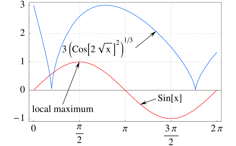
This example produces the conventional Mathematica plot in fig. 1(a). Merely in the last line, a MathPSfrag command is invoked to produce fig. 1(b).

f1[x_] := Sin[x];
f2[x_] := 3*((Cos[2 Sqrt[x]])^2)^(1/3);

rawplot = Plot[{f1[x], f2[x]}, {x, 0, 2 Pi},
      PlotStyle$\to${Hue[1.0], Hue[0.6]}, Frame$\to$True,
      FrameTicks$\to${Pi/2*{0, 1, 2, 3, 4}, Automatic, None, None},
      TextStyle$\to${FontFamily$\to$"Times"}];

SimpleLabel[tip : {_, _}, txt_, txtpos : {_, _}, align : {_, _}] :=  Sequence[
    Arrow[txtpos, tip, HeadScaling$\to$Absolute, HeadLength$\to$8, HeadCenter$\to$0.6],
    Text[txt, txtpos, align]];

textlabels = Graphics[{
        SimpleLabel[{Pi/2, f1[Pi/2]}, "local maximum", {1, -0.5}, {0, 1}],
        SimpleLabel[{7/6Pi, f1[7/6Pi]}, f1[x], {4.2, -0.3}, {-1, 0}],
        SimpleLabel[{4.2, f2[4.2]}, f2[x], {3.5, 1.5}, {1, 0}]
        }];

mygrid = Map[{#, {AbsoluteDashing[{0.1, 1}], GrayLevel[0.5]}} &, {Pi*{1/2, 1,
            3/2}, {1, 2}}, {2}];
exampleplot = Show[rawplot, textlabels, GridLines$\to$mygrid];

Export["ex_nopsfrag.eps", exampleplot, "EPS"]
PSfragExport["ex_auto", exampleplot]

.2 Rotated Text

While Mathematica does not rotate the letters of a rotated Text on screen, both the conventional Export and PSfragExport do the right thing, cf. fig. 3. Furthermore, it is demonstrated, that PSfragExport can apply the option PlotRange$\to$All to the graphics before carrying out the export.

Show[Graphics[{
        Table[Text["Example " <> ToString[Round[phi*180/Pi]],
                   {Cos[phi], Sin[phi]}, {0, 0}, {Cos[phi], Sin[phi]}],
              {phi, 0, 2Pi - 0.01, 2Pi/6}],
        Table[Text[PSfrag["Example " <> ToString[Round[phi*180/Pi]]],
                   {Cos[phi], Sin[phi]}, {0, 0}, {Cos[phi], Sin[phi]}],
              {phi, 2Pi/12, 2Pi - 0.01, 2Pi/6}],
        Circle[{0, 0}, 1]
     }]];
PSfragExport["ex_rot", %, AutoConvertText $\to$ False, PlotRange $\to$ All]

.3 Three-dimensional Knot

Here, the three-dimensional knot in fig. 4 is generated. Note that PSfragExport acting on Graphics3D always implies AutoConvertText$\to$False and AutoPosition$\to$False.

myticks3d = {#, PSfrag[#, Position$\to$"Br"]} & /@ {-1, -0.5, 0, 1, 0.5, 1};
ParametricPlot3D[
    Evaluate[Flatten[{(0.5 + 0.2*Cos[phi/5] + r*Sin[1.7phi]){Cos[phi],
              Sin[phi]}, phi/(5Pi) + r*Cos[1.7 phi]}]],
    {phi, -3Pi, 4Pi}, {r, 0.05, 0.2}, PlotPoints$\to${200, 3}, Ticks$\to${myticks3d, myticks3d, myticks3d}];
PSfragExport["ex_3d", %, RenumberTags$\to$True]

.4 Manual Clone of the Introductory Example

Under the assumption that the automatic export did not work at all, the manual alignment options are used to reproduce fig. 1(b). Moreover, the opportunity to improve the $\cos(\dots)$ label by hand is seized; the corresponding commands below are in italics. The functions f1, f2 and SimpleLabel from the first example have been taken over.

mytickmarks = {
      {N[#], PSfrag[#, Position$\to$"tc"]} & /@ (Pi/2*{0, 1, 2, 3, 4}),
      {N[#], PSfrag[#, Position$\to$"cr"]} & /@ {-1, 0, 1, 2, 3},
      None,
      None};

texstr = "$3\left|\cos \sqrt{4x}\right|^\frac{2}{3}$";

Show[ Plot[
        {f1[x], f2[x]}, {x, 0, 2 Pi}, PlotStyle$\to${Hue[1.0], Hue[0.6]},
        Frame$\to$True, FrameTicks$\to$mytickmarks, GridLines$\to$mygrid,
        DisplayFunction$\to$Identity
        ],
      Graphics[{
        SimpleLabel[{Pi/2, f1[Pi/2]},
          PSfrag["local maximum", Position$\to$"tc"], {1, -0.5}, {0, 1}],
        SimpleLabel[{7/6Pi, f1[7/6Pi]},
          PSfrag[f1[x], Position$\to$"cl"], {4.2, -0.3}, {-1, 0}],
        SimpleLabel[{4.2, f2[4.2]},
          PSfrag[f2[x], Position$\to$"cr", TeXCommand$\to$texstr], {3.5, 1.5}, {1, 0}]
        }],
      DisplayFunction$\to$$DisplayFunction
      ];
PSfragExport["ex_manual", %, AutoConvertText$\to$False, AutoPosition$\to$False]

.5 HoldForm plus CustomTicks

Fig. 7 is a plain example demonstrating that HoldForm can be used to fix the shape of an expression while LinTicks from CustomTicks Caprio (2005) can be used to circumvent the usual stripped decimal “1.” and print a much nicer “1.0” instead.

Plot[(3x - 1)^3, {x, -0.5, 2.5}, PlotStyle$\to$Hue[0.6],
    AxesLabel$\to${x, HoldForm[(3x - 1)^3]},
    Ticks$\to${LinTicks[-0.5, 2.5], LinTicks[-15, 18]}];
PSfragExport["ex_hold", %]

References

- McKay and Moore (1999) W. McKay and R. Moore, TUGboat 20(3) (1999), URL http://www.tug.org/TUGboat/Articles/tb20-3/tb64ross.pdf.
- (2) M. C. Grant and D. Carlisle, The PSfrag system, version 3, URL http://www.ctan.org/tex-archive/macros/latex/contrib/psfrag/pfgguide.ps.
- Wolfram (1999) S. Wolfram, The Mathematica book (4th edition) (Cambridge University Press, New York, NY, USA, 1999), ISBN 0-521-64314-7.
- Wolfram Research, Inc. (2005) Wolfram Research, Inc., Mathematica 5.2 (2005), URL http://www.wolfram.com/.
- (5) J. Große, MathPSfrag v. 1.0, URL http://wwwth.mppmu.mpg.de/members/jgrosse/mathpsfrag/MathPSfrag-1.0.tar.gz.
- Caprio (2005) M. Caprio, Custom tick marks for linear, logarithmic, and general nonlinear axes (2005), URL http://library.wolfram.com/infocenter/MathSource/5599/.