First-Order Modeling and Stability Analysis of Illusory Contours

Abstract

In visual cognition, illusions help elucidate certain intriguing latent perceptual functions of the human vision system, and their proper mathematical modeling and computational simulation are therefore deeply beneficial to both biological and computer vision. Inspired by existent prior works, the current paper proposes a first-order energy-based model for analyzing and simulating illusory contours. The lower complexity of the proposed model facilitates rigorous mathematical analysis on the detailed geometric structures of illusory contours. After being asymptotically approximated by classical active contours, the proposed model is then robustly computed using the celebrated level-set method of Osher and Sethian (J. Comput. Phys., 79:12-49, 1988) with a natural supervising scheme. Potential cognitive implications of the mathematical results are addressed, and generic computational examples are demonstrated and discussed.

Keywords: illusion, illusory contours, energy model, local stability, contour decomposition, real and imaginary, kinks, spans, turns, level-set method, supervision.

Dedicated to David Mumford – A wellspring of inspiration to the young.

1 Introduction

In System Theory [20], input-output analysis has been a major tool for partial or complete identification of black-box systems. In cognitive vision science, the study of various visual illusions follows exactly the same spirit. Cognitive scientists have designed numerous intriguing inputs of image signals, so that the distorted or transformed outputs (as reported by an average human observer) can help reveal some crucial latent properties of the human vision system (see, e.g., the remarkable works of Adelson [1], Knill and Kersten [14, 16], and Kanizsa [11]). Illusory contours are such a well known class of visual illusions, and the current paper develops a mathematical model to characterize, analyze, and simulate generic illusory contours. Our work has been closely inspired by many existent modeling works, especially by Sarti, Malladi, and Sethian [24], and Zhu and Chan [30, 31].

Fig. 1 shows two examples of illusory contours known as Kanizsa triangle and square [11, 24, 30]. The illusory or imaginary white triangle and square pop out almost instantly to a normal observer. The human vision system is capable of interpolating non-existent edges and making meaningful visual organization of both the real and imaginary edge segments. From the viewpoints of modeling and computation, such illusory perception has also been called segmentation with missing boundaries [24], and is closely related to some earlier works (e.g., [18, 19]).

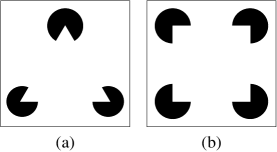
Figure 1: Two classical examples of illusory contours: Kanizsa’s triangle and square.

Qualitatively, the perception of illusory contours can be deciphered by the Gestalt framework [10, 11]. In a typical example of illusory contours, the illusory target objects share the same gray level as their background and become invisible to ordinary detectors. The illusory targets however do leave their footprints, mainly through the cues of occlusion, e.g., the visible corners in Fig. 1. An average human vision system can organize these cues and develop a so-called 2.1-D sketch of the scene [19], i.e., to separate and complete objects in ordered (according to the relative depth to a viewer) multiple layers. The multi-layer sketch of Kanizsa’s triangle is displayed in Fig. 2, for example. We also refer the reader to the recent work of Shen [29] on an abstract study of the occlusion phenomenon and 2.1-D models.

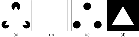
Figure 2: Multi-layer decomposition of Kanizsa’s triangle: (a) image of Kanizsa’s triangle, (b) far background, (c) three disks in the middle range, and (d) the illusory triangle closest to a viewer.

Quantitatively, however, it is a nontrivial task to properly model and compute illusory contours. There are two notable recent works that have primarily influenced the present work in developing plausible mathematical models and robust computational schemes.

In [24], Sarti, Malladi, and Sethian first proposed a variational-PDE model for computing illusory contours based on a reference point within an image. Given a reference point which models the focus of visual attention, a surface is then constructed and flattened except along the existing real edges. The level sets of the surface function are able to connect the imaginary contours. Define the edge indicator function by [24]

$$g(x)=g(x_{1},x_{2})=\frac{1}{1+(\lvert\nabla G_{\sigma}(x)*u(x)\rvert/\beta)^{2}},$$

$$G_{\sigma}(\xi)=\frac{\exp(-(\xi/\sigma)^{2})}{\sigma\sqrt{\pi}}.$$

Then the model is to minimize the $g$-weighted area of the surface $S:x=(x_{1},x_{2})\rightarrow(x_{1},x_{2},\Phi)$:

$$\min_{\Phi}\int_{\Omega}g(x)\sqrt{1+\Phi_{x_{1}}^{2}+\Phi_{x_{2}}^{2}}dx.$$

Our model shares a similar computational formulation, but is more self-contained in terms of modeling and analysis since it is directly built on curves rather than on reference points and surfaces. (We must point out that, in visual cognition, attention focuses do play important roles in a number of cognitive tasks [11].)

Later in [30], Zhu and Chan proposed a more complex level-set based variational model. Let $u:\Omega\rightarrow\mathbb{R}$ be an image defined on the domain $\Omega$, with $u=1$ on the objects and $u=-1$ otherwise. The key component of Zhu and Chan’s model is the signed distance function from solving the eikonal equation :

$$\frac{\partial d}{\partial t}=\text{sign}(u)(1-|\nabla d|),$$

with the initial data $d(x,t=0)=u(x)=u(x_{1},x_{2})$. Their variational model is then to minimize the following energy for the level-set function $\phi$ which codes the desired illusory contours:

$$\begin{split}E(\phi)=&\int_{\Omega}\left((1+\mu C(d)\kappa^{+}(d))|d|\delta(\phi)\lvert\nabla\phi\rvert+\lambda H(d)H(\phi)\right)dx\\ &+\int_{\Omega}\left(a+b\left|\nabla\cdot\left[\frac{\nabla\phi}{|\nabla\phi|}\right]\right|^{2}\right)|\nabla\phi|\delta(\phi)dx,\end{split}$$ (1)

where $\delta$ denotes Dirac’s delta, $H$ the Heaviside function, and $C$ a $C^{1}$ differentiable cut-off function. The $|d|\delta(\phi)\lvert\nabla\phi\rvert$ term measures the distance from the zero level-set to the existent boundaries and $C(d)\kappa^{+}(d)|d|\delta(\phi)\lvert\nabla\phi\rvert$ measures the distance to concave corners. The second term of the first integral measures the overlap between the existent objects and the interior of $\phi$. The last integral represents Euler’s elastica energy which was first proposed by Mumford [17], and later applied to geometric image inpainting by Chan, Kang, and Shen [2], and Esedoglu and Shen [8]. Zhu and Chan [30] showed outstanding performance of this model for several general examples. Our proposed model is much less complex than this high-order geometric model, and is also independent of the signed distance function. The essence of our proposed model is to be able to capture the most salient features of illusory perception in a simple and analyzable manner, at the unsurprising cost of losing certain high-order details. (Zhu and Chan [31] later also employed prior shape information to capture illusory contours.)

Mainly inspired by these pioneering works on quantitative modeling, we propose a new energy-based model for studying illusory contours. The model is directly formulated on admissible contours and does not depend upon reference points nor their associated surfaces. The model has a much lower order of complexity which however yields good leading-order approximation to most generic illusory contours (with exact capturing in the canonical cases of Kanizsa’s triangle or square). The relationship between this new model and the more complex models of Zhu and Chan is formally analogous to that between the first-order and second-order Taylor expansions in Calculus. Most remarkably, the lower complexity of the new model allows to almost completely characterize the structures of illusory contours, which provides a solid stepstone towards more general quantitative analysis in the future. To our best knowledge, such rigorous characterization has been unprecedented in the literature.

The second major feature of the new model is that in terms of computation, it can be efficiently implemented by classical active contours and level-set based algorithms of Osher and Sethian [22, 21, 26, 25]. In particular, we introduce a key but natural step of supervision for capturing robustly illusory contours, which can also be considered as an innate component of the new model itself.

The paper has been organized as follows. In Section 2, we develop and analyze the new model for illusory contours that emerge from any generic configuration of real objects. We are able to rigorously characterize the geometric structures of illusory contours when identified as the local minima of the proposed model. In Section 3, the model is further extended to process configurations with real contours. In Section 4, an approximate or relaxed model is then developed based on the classical active-contour model of Kass, Witkin and Terzopoulos [12], which allows the proposed model to be actually computed via asymptotic approximation. In Section 5, the level-set method of Osher and Sethian [21, 22, 26] is employed to compute the stable local minima of the model, under the help of a key step of supervision. Finally, the details of numerical implementation as well as the computational performance of the proposed model are provided in Section 6.

2 Illusory contours as stable local minima and characterization

In this section, we propose a contour-based energy model, and model illusory contours as the local minima of such an energy. The particular form of the energy allows detailed and rigorous analysis of the geometric and topological structures of admissible local minima. Such in-depth mathematical characterization is, to our best knowledge, unique in the literature.

Note that a local minimum corresponds to an energy valley and is stable only to local perturbations. This differs our model from many other efforts in modeling illusory contours as global minima. Aiming at local instead of global minima has also been motivated by cognitive sensitivities of illusory perception (of light, geometry, or objects, etc) to various factors including visual attention, focus points, orientations, and scaling, etc. Such visual factors may disrupt or erase an observer’s ongoing illusory experience, while global minima often remain stable to these external perturbations.

In later sections we then develop an efficient level-set-based computational algorithm that supports stable stagnation at such local minima.

2.1 Kinks, outer and inner spans $\theta$, and a generic configuration $Q$

Let $\Omega$ denote the entire open image domain, which could be the complete plane $\mathbb{R}^{2}$ or a finite rectangle area. Let $Q=\{Q_{i}\mid i=1:k\}$ be a configuration of disjoint compact domains whose boundaries are piecewise-$C^{2}$ simple closed curves. Denote the boundaries by

$$\partial Q=\partial Q_{1}\cup\partial Q_{2}\cup\cdots\cup\partial Q_{k}.$$

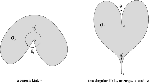
Figure 3: Left panel: a generic kink $y$ with outer span $\theta_{y}>0$ and inner span $\theta^{\ast}_{y}=2\pi-\theta_{y}>0$. Right panel: two examples of singular kinks or cusps; an inward cusp at $z$ with $\theta^{\ast}_{z}=0$ and an outward cusp $x$ with $\theta_{x}=0$. The current work discusses generic configurations containing only generic kinks. Perceptual effects of cusps have scarcely been experimented in visual cognition.

Definition 2.1 (A kink and its outer span $\theta$ and inner span $\theta^{\ast}$).

A point $y\in\partial Q$ is said to be a kink if the two tangent lines from the two sides are not identical. If $y$ is a kink, its outer span $\theta_{y}$ is the angle between the two tangent lines when moving continuously from one arm to the other outside $Q$ (see Fig. 3). We further define $\theta^{\ast}_{y}=2\pi-\theta_{y}$ to be the inner span. For a non-degenerate kink $y$, both $\theta_{y}$ and $\theta_{y}^{\ast}$ must be positive.

A cusp is a singular kink point $y$ for which either the outer span $\theta_{y}=0$ or the inner span $\theta_{y}^{\ast}=0$ (see Fig. 3). It will be interesting in vision psychology to understand the cognitive effects of cusps in various scales. In the current work we shall assume that the given configuration $Q$ only contains generic kinks so that $\theta_{y},\theta^{\ast}_{y}>0$. Such a configuration $Q$ is said to be generic consequently. Almost all classical examples correspond to generic configurations.

Definition 2.2 (Kink set $K$ and minimum spans $\theta_{\min{}}$ and $\theta^{\ast}_{\min{}}$).

Let $Q\subset\Omega$ be a generic configuration. Define its kink set $K[Q]$ to be the collection of all kinks of $Q$, and its minimum outer span by

$$\theta_{\min{}}=\theta_{\min{}}[Q]=\min\{\theta_{y}\mid y\in K[Q]\},$$

and minimum inner span by

$$\theta^{\ast}_{\min{}}=\theta^{\ast}_{\min{}}[Q]=\min\{\theta_{y}^{\ast}\mid y\in K[Q]\}=\max\{2\pi-\theta_{y}\mid y\in K[Q]\}.$$

Since $\partial Q$ is compact and piecewise $C^{2}$, $K[Q]$ must be finite and both $\theta_{\min{}}$ and $\theta^{\ast}_{\min{}}$ are positive.

2.2 Real and imaginary decomposition of a contour

Let $\Gamma$ be any piecewise $C^{2}$ simple closed curve in $\Omega$ that does not intersect the interior of $Q$. Define its real and imaginary parts by

$$\Gamma_{\mathrm{re}}=\Gamma\cap\partial Q,\qquad\Gamma_{\mathrm{im}}=\Gamma\setminus\partial Q.$$ (2)

For an illusory contour $\Gamma$, the imaginary part corresponds precisely to the illusory interpolation (Fig. 4). (The names “real” and “imaginary” have been formally motivated by complex analysis in which a complex number $z$ can be decomposed into real and imaginary parts: $z=z_{\mathrm{re}}+\sqrt{-1}\;z_{\mathrm{im}}$.)

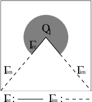
Figure 4: Decomposition of $\Gamma$ into real and imaginary parts (partial view of Kanizsa’s triangle).

Notice that since both $\Gamma$ and $\partial Q$ are compact and thus closed sets, $\Gamma_{\mathrm{re}}$ must be closed in $\Omega$ and $\Gamma_{\mathrm{im}}$ relatively open in $\Gamma$. We shall only consider a curve $\Gamma$ for which $\Gamma_{\mathrm{im}}$ contains finitely many connected components to avoid unnecessary technicalities:

$$\Gamma_{\mathrm{im}}=\gamma^{1}_{\mathrm{im}}\cup\gamma^{2}_{\mathrm{im}}\cup\cdots\cup\gamma^{m}_{\mathrm{im}}.$$

Since $\Gamma_{\mathrm{im}}=\Gamma\cap Q^{c}$, the intersection of a simple closed (and thus locally connected) curve and an open domain, $\Gamma_{\mathrm{im}}$ must be locally connected [13]. Consequently, each connected component $\gamma^{j}_{\mathrm{im}}$ must be a connected curve segment with at most two endpoints. In the current work, we assume that the two endpoints are distinct. (Otherwise, the entire curve $\Gamma$ becomes a loop which touches $\partial Q$ only at a single point. Such a loop can easily shrink to decrease the energy to be proposed immediately next, and is hence irrelevant to the local minima.) Let $\partial\gamma^{j}_{\mathrm{im}}$ denote the two boundary endpoints, and $\partial\Gamma_{\mathrm{im}}=\partial\gamma_{\mathrm{im}}^{1}\cup\cdots\cup\partial\gamma_{\mathrm{im}}^{m}$.

2.3 Energy model and the structural theorem for local minima

For a given generic configuration $Q$ in a 2-D open domain $\Omega$, define the class of admissible curves

$$\mathcal{C}=\{\Gamma\mid\mbox{$\Gamma$ is simple closed, piecewise $C^{2}$ with finitely many pieces, and $\Gamma\cap Q^{\circ}=\mathrm{empty}$}\}.$$ (3)

For any admissible curve $\Gamma\in\mathcal{C}$, we define the energy

$$E_{o}[\Gamma]=E_{o}[\Gamma\mid\alpha,\beta]=\alpha\int_{\Gamma_{{\mathrm{re}}}}ds+\beta\int_{\Gamma_{{\mathrm{im}}}}ds,$$ (4)

where $s$ denotes the arc-length parameter and $0<\alpha\ll\beta$. The subscript “o” in $E_{o}$ signifies that this energy is for object-based configuration $Q$. In the next section, we will introduce an energy $E_{c}$ for contour-based configurations. Notice that $E_{o}$ is the weighted sum of the lengths of ${\Gamma_{{\mathrm{re}}}}$ and ${\Gamma_{{\mathrm{im}}}}$. We are interested in the behavior and characteristics of the local minimizers to $E_{o}$, in particular, in how well they can quantify more familiar features of illusory contours in visual cognition, which have often been subconsciously processed by human observers.

Lemma 2.3.

Let $\Gamma\in\mathcal{C}$ be a local minimizer of $E_{o}$. Then each connected component of ${\Gamma_{{\mathrm{im}}}}$ must be a straight line segment.

Proof.

Suppose otherwise that one connected component $\gamma$ of ${\Gamma_{{\mathrm{im}}}}$ is not a straight line segment. Then there must exist at least one point $b\in\gamma$, within any of whose small neighborhoods, there can be found two points $a,c\in\gamma$ on the two sides of $b$ such that $\{a,b,c\}$ are not collinear. We then replace $\gamma|_{[a,c]}$ by the straight line segment joining $a$ and $c$. Since $\Gamma$ and hence $\gamma$ are piecewise $C^{2}$ and $\gamma\subset Q^{c}$ (an open set), as long as the neighborhood is small enough, the straight line substitute does not intersect the rest of $\Gamma$ nor $Q$. Denote the new curve after such a micro-surgery by $\Gamma^{\prime}$. Then $\Gamma^{\prime}\in\mathcal{C}$ and $E_{o}[\Gamma^{\prime}]<E_{o}[\Gamma]$ since the two only differ in between $a$ and $c$. This contradicts to the assumption that $\Gamma$ is a local minimizer since such micro-surgeries can occur in any local neighborhood of $b$. ∎

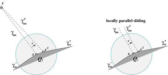
Figure 5: Local perturbation at a junction point $x\in\partial\Gamma_{\mathrm{im}}\subset\partial Q$ can be approximated (in the first order of the displacement distance $\varepsilon$) by a simple parallel translation of the attached imaginary ray $\gamma_{\mathrm{im}}$, due to Lemma 2.3 and the same mechanism that makes direct solar rays appear approximately parallel when reaching onto the Earth. Parallel shifting simplifies most computation.

In the following analysis, the local perturbation of a junction point $x\in\partial\Gamma_{\mathrm{im}}$ along $\partial Q$ (see $x\to x^{\varepsilon}$ in Fig. 5) has always been accomplished by a simple parallel translation of the attached imaginary ray $\gamma_{\mathrm{im}}$. This is justified by the preceding lemma, as well as the fact that when the other endpoint $y$ is relatively far away, the perturbed imaginary ray $\overline{yx^{\varepsilon}}$ due to $x\to x^{\varepsilon}$ is parallel to $\overline{yx}$ in the first order (of $\varepsilon$) within small neighborhoods of $x$ (see Fig. 5 and its caption).

Lemma 2.4 (Two distinct imaginary rays cannot share a hinge).

Suppose $\Gamma\in\mathcal{C}$ is a local minimizer to $E_{o}=E_{o}[\cdot|\alpha,\beta]$, and $\gamma^{1}$ and $\gamma^{2}$ are two distinct connected components (which are straight line segments by the preceding lemma). Then there exists some critical ratio $r_{c}$, such that as long as $r=\alpha/\beta<r_{c}$, $\partial\gamma^{1}\cap\partial\gamma^{2}$ must be empty.

Proof.

(See the companion illustration in Fig. 6) Otherwise, assume that $\gamma^{1}$ and $\gamma^{2}$ share a hinge at a point $z$ (i.e., the point $O$ in the figure). Then $z$ must be a real point, and one can assume that $z\in\partial Q_{j}$ for some unique $j$.

Locally in a small diskette neighborhood of $z$, the two straight rays $\gamma^{1}$ and $\gamma^{2}$ segment the disk into two parts: an “inner” part that intersects with $Q_{j}$ and an “outer” part. Let $\theta$ denote the outer span angle.

First suppose $\theta\in(0,\pi)$. Then any corner-cutting local deformation near $z$ (as shown in the left panel of Figure 6) can decrease energy $E_{o}$ since the the real part of the energy is unchanged but the imaginary one shrinks. Thus this scenario cannot occur.

Then one must have $\theta\geq\pi$. For $\partial Q_{j}$, similarly there are two real tangent rays at $z$, denoted by $\mu^{1}$ and $\mu^{2}$, so that the acute cone of $\mu^{1}$ and $\gamma^{1}$ contains neither of the other two rays. Let $\phi_{i}$ denote the acute angle between $\mu^{i}$ and $\gamma^{i}$, $i=1,2$. Without loss of generality, assume that $\phi_{1}\leq\phi_{2}$. Since

$$\phi_{1}+\phi_{2}\leq(2\pi-\theta)-\theta^{\ast}_{\min{}}\leq\pi-\theta^{\ast}_{\min{}},$$

one has

$$\phi_{1}=\min(\phi_{1},\phi_{2})\leq\frac{\pi}{2}-\frac{\theta^{\ast}_{\min{}}}{2}.$$

Then as shown in the right panel of Fig. 6, a small parallel sliding (with perpendicular distance $\varepsilon$) of the root of the imaginary ray $\gamma^{1}$ along the real edge of $\partial Q_{j}$ in the direction of $\mu^{1}$ will introduce an energy increment of:

$$\alpha\frac{\varepsilon}{\sin\phi_{1}}-\beta\frac{\varepsilon}{\tan\phi_{1}}=\frac{\varepsilon\beta}{\sin\phi_{1}}\left(\frac{\alpha}{\beta}-\cos\phi_{1}\right).$$

Define $r_{c}=\cos(\pi/2-\theta^{\ast}_{\min{}}/2)=\sin(\theta^{\ast}_{\min{}}/2)>0$. Then as long as $r=\alpha/\beta<r_{c}$, the leading order of energy increment is in fact negative, which again contradicts to the given assumption. To conclude, as long as $r<r_{c}$, two distinct imaginary line segments cannot share a hinge. ∎

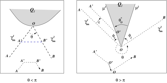
Figure 6: Companion illustration for the proof of Lemma 2.4: Two distinct imaginary rays $\gamma_{\mathrm{im}}^{1}$ and $\gamma_{\mathrm{im}}^{2}$ (of a local minimum contour $\Gamma$) cannot share a common hinge $O$ (Lemma 2.4). Left panel: if $\theta<\pi$, a local perturbation of $\overline{AOB}$ to $\overline{AA^{\prime}B^{\prime}B}$ decreases the total energy $E_{o}$. Right panel: if $\theta\geq\pi$, a local perturbation of $\overline{AOB}$ to $\overline{A^{\prime}O^{\prime}OB}$ still decreases the total energy (see the computation in the proof of Lemma 2.4).

Definition 2.5 (Junction set $J{[\Gamma]}$ and a turn $\phi_{z}$ at a junction point $z$).

For a minimizer $\Gamma\in\mathcal{C}$, we define its junction set to be

$$J[\Gamma]=\partial\Gamma_{\mathrm{im}},\qquad\mbox{i.e., all endpoints of imaginary segments.}$$

By definition, one must have $J[\Gamma]\subseteq\partial Q$. For any junction point $z\in J[\Gamma]$, in one direction $\Gamma$ goes to a uniquely associated imaginary ray, and let ${\boldsymbol{t}}_{\mathrm{im}}={\boldsymbol{t}}_{\mathrm{im}}(z)$ denote this outgoing unit vector of orientation, and in the other direction comes a curve segment of $\Gamma_{\mathrm{re}}$ (according to the preceding lemma) and let ${\boldsymbol{t}}_{\mathrm{re}}={\boldsymbol{t}}_{\mathrm{re}}(z)$ denote this incoming unit vector of orientation (see Fig. 7). The turn at $z$ is then defined to be the angle:

$$\phi_{z}=\arccos({\boldsymbol{t}}_{\mathrm{im}}\cdot{\boldsymbol{t}}_{\mathrm{re}})\in[0,\pi].$$

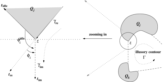
Figure 7: A permissible geometric layout at a junction point $z\in J[\Gamma]$ with the turn $\phi_{z}<\pi/2$ and idle turn $\phi_{z}\geq\pi/2$, according to the results established in Lemmas 2.6 and 2.9.

Lemma 2.6 (Acute turns at junction points).

Suppose $\Gamma\in\mathcal{C}$ is a local minimum of $E_{o}$ and $z\in J[\Gamma]$ is a junction point. Then the turn $\phi_{z}<\pi/2$.

Proof.

Suppose otherwise that $\phi_{z}\geq\pi/2$. Then if one slides the root $z$ of the imaginary ray $\gamma_{\mathrm{im}}$ along the incoming part of $\Gamma_{\mathrm{re}}$ while keeping the imaginary rays parallel, as well as other parts of $\Gamma$ intact, as in the left panel of Fig. 8, the leading order energy increment becomes:

$$-\beta\frac{\varepsilon}{\tan(\pi-\phi_{z})}-\alpha\frac{\varepsilon}{\sin(\pi-\phi_{z})}<0,$$

which contradicts to the assumption of $\Gamma$ being a local minimum. (Notice that in the critical case when $\phi_{z}=\pi/2$, the first term degenerates into a second-order change $O(\varepsilon^{2})$. Thus the result still holds due to the second term.) ∎

This lemma has an intuitive interpretation in terms of visual cognition. Illusory contours more or less are smooth and straight extrapolations of existing real boundaries [4, 5], and consequently the turns at the junction points should generally be as small as possible.

Definition 2.7 (Maximum turn of a local-minimum contour $\Gamma$).

Suppose $\Gamma\in\mathcal{C}$ is a local minimum of $E_{o}$. Define the maximum turn $\phi_{\max{}}$ of $\Gamma$ by

$$\phi_{\max{}}=\max\{\phi_{z}\mid z\in J[\Gamma]\}.$$

Then the preceding lemma implies that $\phi_{\max{}}<\pi/2$.

Definition 2.8 (Idle angle $\phi^{\mathrm{idle}}$ at a junction point).

Let $\Gamma\in\mathcal{C}$ be a local minimum to $E_{o}$, and $z\in J[\Gamma]$ a junction point. Define the imaginary tangent ${\boldsymbol{t}}_{\mathrm{im}}={\boldsymbol{t}}_{\mathrm{im}}(z)$ as in Definition 2.5. Further define the idle tangent ${\boldsymbol{t}}_{\mathrm{idle}}={\boldsymbol{t}}_{\mathrm{idle}}(z)$ to be the unit outgoing tangent vector of $\partial Q\setminus\Gamma_{\mathrm{re}}$ (i.e., the idle real boundaries that do not participate in the formation of $\Gamma$) at $z$ (see Fig. 8). Define the idle angle at $z$ by

$$\phi^{\mathrm{idle}}_{z}=\arccos({\boldsymbol{t}}_{\mathrm{idle}}\cdot{\boldsymbol{t}}_{\mathrm{im}}).$$

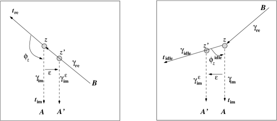
Figure 8: Companion illustration for the proofs of Lemmas 2.6 and 2.9. Left panel: the turn $\phi_{z}$ at a junction point $z\in J[\Gamma]$ cannot be blunt, otherwise the local perturbation of $z$ to $z^{\prime}$ and $\gamma_{\mathrm{im}}$ to $\gamma_{\mathrm{im}}^{\varepsilon}$ decreases both the real and imaginary energies in $E_{o}$. Right panel: the idle turn $\phi^{\mathrm{idle}}_{z}$ cannot be acute for sufficiently small $\alpha/\beta$, otherwise the perturbation shown will cause a net drop in the total energy $E_{o}$ (see the computation in the proof of Lemma 2.9).

Lemma 2.9 (Behavior of idle angles at junctions).

Suppose $\Gamma\in\mathcal{C}$ is a local minimum to $E_{o}[\cdot\mid\alpha,\beta]$ for any $\alpha,\beta>0$, and $z\in J[\Gamma]$ is one of its junction point. Then $\phi^{\mathrm{idle}}_{z}\geq\pi/2$.

Proof.

Suppose otherwise that $\phi_{z}^{\mathrm{idle}}<\pi/2$. Then if one slides the root $z$ of the imaginary ray $\gamma_{\mathrm{im}}$ along the outgoing idle part of $\partial Q\setminus\Gamma_{\mathrm{re}}$ while keeping the imaginary rays parallel, as well as other parts of $\Gamma$ intact, as in the right panel of Fig. 8, the leading order energy increment becomes:

$$\alpha\frac{\varepsilon}{\sin\phi^{\mathrm{idle}}_{z}}-\beta\frac{\varepsilon}{\tan\phi^{\mathrm{idle}}_{z}}=\frac{\varepsilon\beta}{\sin\phi_{z}^{\mathrm{idle}}}\left(\frac{\alpha}{\beta}-\cos(\phi^{\mathrm{idle}}_{z})\right).$$ (5)

Since $\Gamma$ is a local minimum for any $\alpha,\beta>0$, one must have

$$-\cos(\phi^{\mathrm{idle}}_{z})\geq 0,\qquad\mbox{or}\qquad\phi^{\mathrm{idle}}_{z}\geq\pi/2.$$

∎

Combining all the characterizations established in the lemmas of this section, we are ready to state the main theorem of this paper.

Theorem 2.10 (Characterization of a local minimum).

Let $Q$ be a generic configuration on an open domain $\Omega$, and $\theta_{\min{}},\theta^{\ast}_{\min{}}>0$ its minimum outer and inner spans. Suppose a given simple closed curve $\Gamma\in\mathcal{C}$ satisfies the following structural conditions:

1. (Imaginary behavior) each connected component $\gamma_{\mathrm{im}}$ of $\Gamma_{\mathrm{im}}$ is a straight line segment, and no two distinct components share a common hinge;

2. (Junction behavior) at any junction point $z\in J[\Gamma]$, the turn $\phi_{z}<\pi/2$, and the idle angle $\phi^{\mathrm{idle}}_{z}\geq\pi/2$.

Let $\phi_{\max{}}$ denote the maximum turn on $J[\Gamma]$. Then there exists a critical ratio $r_{c}=r_{c}(\theta_{\min{}},\phi_{\max{}})<1$, such that for any $\alpha$ and $\beta$ with $r=\alpha/\beta<r_{c}$, $\Gamma$ is a local minimum to the energy $E_{o}[\cdot\mid\alpha,\beta]$.

Proof.

We shall only outline the main steps of the proof and leave the details to the reader, which are very similar to the proofs of the above ensemble of lemmas. Let $J[\Gamma]$ denote the junction set of such a given $\Gamma$, and define

$$\Gamma_{\mathrm{re}}^{\circ}=\Gamma_{\mathrm{re}}\setminus J[\Gamma].$$

Then $\Gamma$ is segmented into three distinct parts:

$$\Gamma=\Gamma_{\mathrm{im}}\cup\Gamma_{\mathrm{re}}^{\circ}\cup J[\Gamma],$$

each of which leads to a distinct energy variation pattern due to local admissible perturbations.

First, it is easy to see that under Condition (i) any local perturbations at a point of $\Gamma_{\mathrm{im}}$ will increase the energy.

Next, $\Gamma_{\mathrm{re}}^{\circ}$ can be further partitioned into kink points $\Gamma_{\mathrm{re}}^{\circ}\cap K[Q]$ and the majority rest of smooth points. At a smooth point $y$, any generic local variation drifts a real local segment $\gamma$ into $Q^{c}$ and converts it into an imaginary one, and hence introduces a net leading-order energy increment of $(\beta-\alpha)\int_{\gamma}ds$, which is always positive for $r=\alpha/\beta<1$. At a kink point $y$ on $\Gamma_{\mathrm{re}}^{\circ}$, one defines $r_{1}=\sin\theta_{\max{}}/2>0$. Then simple trigonometric calculus shows that for any $\alpha$ and $\beta$ with $\alpha/\beta<r_{1}$, any local admissible displacement of the kink point always increases the energy.

Finally, one turns to the local perturbations at any junction point $z\in J[\Gamma]$. By Condition (ii) on the acute turns, one must have that the maximum turn $\phi_{\max{}}<\pi/2$. Define $r_{2}=\cos\phi_{\max{}}>0$. Then trigonometric calculus shows that any local drifting of $z$ into the incoming real contour $\Gamma_{\mathrm{re}}$ will increase the energy as long as $\alpha/\beta<r_{2}$. On the other hand, any local drifting of $z$ into the idle real edge $\partial Q\setminus\Gamma_{\mathrm{re}}$ always increases energy due to Condition (ii) on $\phi^{\mathrm{idle}}_{z}\geq\pi/2$, for any $\alpha,\beta>0$. The details are very similar to the proofs of Lemmas 2.6 and 2.9.

In combination, one defines the critical ratio $r_{c}=\min(r_{1},r_{2},1)$. Then for any $\alpha$ and $\beta$ with $\alpha/\beta<r_{c}$, the above analysis in all the three scenarios shows that the energy always increases under any local perturbations of $\Gamma$. Thus $\Gamma$ must be a local minimum to $E_{o}[\cdot\mid\alpha,\beta]$. ∎

By this theorem, it is straightforward to establish the following corollary, which demonstrates that local minima of $E_{o}$ are indeed reasonable models for illusory contours, at least in terms of the leading-order approximation.

Corollary 2.11.

Both Kanizsa’s triangle and square are local minimizers to $E_{o}[\Gamma\mid\alpha,\beta]$ for sufficiently small $\alpha/\beta$.

Remark 2.12.

In the preceding main theorem, only the condition $\phi^{\mathrm{idle}}_{z}\geq\pi/2$ could be relaxed to $\phi^{\mathrm{idle}}_{z}\geq\pi/2-\delta$ for some constant $\delta=\delta(\alpha,\beta)\geq 0$ with $\delta\to 0$ as $r=\alpha/\beta\to 0$ (due to Eqn. (5)). The preceding lemmas show that all the other conditions are necessary and cannot be further relaxed.

3 Real contour bundles and object-contour mixtures

In this section, we briefly discuss contour-based illusory contours, as well as those arising from a mixture configuration of both objects and contours. Computationally, however, it can be handled by exactly the same scheme for the object-based model, as to be numerically demonstrated later on.

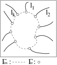
Figure 9: Decomposing a candidate contour $\Gamma$ into its real part $\Gamma_{\mathrm{re}}$ and imaginary part $\Gamma_{\mathrm{im}}$.

Let $L=\{l_{i}\}^{n}_{i=1}$ be a bundle of disjoint compact contour segments on a given open image domain $\Omega$. To be distinguished from illusory contours, each $l_{i}$ shall be called a real contour (see Fig. 9). Let $\partial l_{i}=\{a_{i},b_{i}\}$ denote the two endpoints of $l_{i}$. Define

$$\partial L=\cup_{i=1}^{n}\partial l_{i}=\cup_{i=1}^{n}\{a_{i},b_{i}\},\qquad L^{\circ}=L\setminus\partial L.$$

As for object-based illusory contours, we define the class of contour-based admissible contours by

$$\mathcal{C}_{c}=\{\Gamma\mid\mbox{$\Gamma$ is simple closed, piecewise $C^{2}$, and $\Gamma\cap L^{\circ}=$empty}\}.$$

For each admissible contour $\Gamma\in\mathcal{C}_{c}$, we define, in the same spirit of the previous object-based case, the real-imaginary decomposition (Fig. 9):

$$\Gamma_{\mathrm{re}}=\Gamma\cap\partial L,\quad\Gamma_{\mathrm{im}}=\Gamma\setminus\partial L=\Gamma\setminus\Gamma_{\mathrm{re}}.$$

As a result, the previous object-based energy $E_{o}$ is modified to the following contour-based:

$$E_{c}[\Gamma]=-\alpha\mathcal{H}^{0}({\Gamma_{{\mathrm{re}}}})+\beta\int_{\Gamma_{{\mathrm{im}}}}ds=-\alpha\mathcal{H}^{0}({\Gamma_{{\mathrm{re}}}})+\beta\int_{\Gamma}ds,$$ (6)

with $\alpha,\beta>0$. Here $\mathcal{H}^{0}$ denotes the 0-dimensional Hausdorff measure, or equivalently, the atomic counting measure.

The major difference of $E_{c}$ from the previous object-based energy $E_{o}$ resides in the first negative term. Under this new formulation, any real end point from $\partial L$ acts like an energy basin, in order to be able to anchor prospective illusory contours.

The local minimizers of $E_{c}$ are much easier to characterize.

Theorem 3.1.

$\Gamma\in\mathcal{C}_{c}$ is a local minimizer with a non-empty imaginary part $\Gamma_{\mathrm{im}}$ if and only if it is a polygon whose vertices are all anchored within $\partial L$.

Proof.

First suppose $\Gamma$ is a local minimizer with a non-empty imaginary part $\Gamma_{\mathrm{im}}$. For any connected component $\gamma$ of $\Gamma_{\mathrm{im}}$, the same argument as in Lemma 2.3 applies since a local perturbation of $\gamma$ only modifies the length integral in the $\beta$-term. Thus $\gamma$ must be a straight line segment. Since $\gamma$ is arbitrary, $\Gamma\in\mathcal{C}_{c}$ has to be a polygon whose vertices are anchored within $\partial L$.

Conversely, suppose $\Gamma\in\mathcal{C}_{c}$ is a polygon whose vertices belong to $\partial L$. Any local variation within a side $\gamma$ of $\Gamma$ increases the $\beta$-term line integral while leaving the atomic $\alpha$-term unchanged, since $\gamma$ is straight. On the other hand, any nonzero local perturbation of a vertex of $\Gamma$ will drift it into $\Omega\setminus L$ (since the perturbation must be kept within the admissible class $\mathcal{C}_{c}$), and consequently cause a leading-order energy increment of $\alpha$. Hence $\Gamma$ is a local minimizer, and the proof is complete. ∎

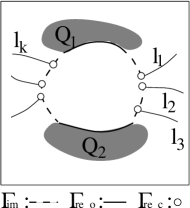
Figure 10: Decomposition of a candidate curve $\Gamma$ in an object-contour mixture configuration.

Finally, some examples in the literature also involve illusory contours from a mixture configuration of both objects and contours. For this reason, we consider a mixture model briefly. Consider an image which is composed of compact and mutually disjoint real objects $Q$ and real contours $L$. Let $\Gamma$ be an admissible piecewise $C^{2}$ simple closed curve in $\Omega$ that does not intersect $Q^{\circ}\cup L^{\circ}$ (defined previously). We define the real and imaginary part of $\Gamma$ as follows:

$$\Gamma_{{\mathrm{re}}} = \Gamma_{\text{re\_o}}\cup\Gamma_{\text{re\_c}}=(\Gamma\cap\partial Q)\cup(\Gamma\cap\partial L),$$

$$\Gamma_{{\mathrm{im}}} = \Gamma\setminus\Gamma_{\mathrm{re}}=\Gamma\setminus(\partial Q\cup\partial L).$$

Notice that here the real part has been further categorized into object-based real part $\Gamma_{\text{re\_o}}$ and contour-based real part $\Gamma_{\text{re\_c}}$. We then define a mixture energy functional $E_{m}$ in the form of:

$$E_{m}[\Gamma]=\alpha_{o}\int_{\Gamma_{\text{re\_o}}}ds-\alpha_{c}\mathcal{H}^{0}(\Gamma_{\text{re\_c}})+\beta\int_{\Gamma_{\mathrm{im}}}ds.$$

where $0<\alpha_{o}\ll\beta$ and $\alpha_{c}>0$.

The characterization of a local minimizer to this mixture energy can be readily obtained from a straightforward combination of the previous two major theorems. In particular, for example, if $\Gamma$ is a local minimizer, then two distinct connected components $\gamma^{1}$ and $\gamma^{2}$ of the imaginary part can share a common hinge, but the hinge point must belong to $\partial L$ and not to $\partial Q$.

Next we discuss how to compute these models in real applications. In particular, we will demonstrate numerically that for practical applications, a single relaxed model is sufficient to handle all the previous three theoretical models of $E_{o},E_{c},$ and $E_{m}$.

4 Relaxation of the model: approximation by active contours

The main models have been built upon the real-imaginary decomposition of any candidate contour $\Gamma$, which in turn depends upon the identifiability of the real edge set $\partial Q$. Hence arise two major practical issues for implementing these models realistically. First, for general images, one has to perform a pre-processing of edge detection in order to obtain $\partial Q$, which is easier for binary images but highly nontrivial for general continuous-tone images. Second, even provided with $\partial Q$, it is well known that direct computation of curves is highly challenging due to the densening or coarsening effects of discrete points as well as potential topological changes like splitting and merging.

The current section resolves the first issue, while the next section will address the second.

The main result of this section is to show that the edge-detection process can be implicitly integrated into an approximate model, which surprisingly turns out to be the more familiar active contour model [7, 6, 12, 15]. That is, the proposed new model for illusory contours can be asymptotically approximated by active contours when restricted in the class of admissible contours $\mathcal{C}$.

First consider an ideal binary image $u(x)=\chi_{Q}(x)$, i.e., the characteristic function of a generic configuration $Q$. Let $\eta(x)$ be any $C^{\infty}$ positive function which is compactly supported on the unit disk in the plane, and for any scale $\sigma>0$, define the mollifier $\eta_{\sigma}(x)=\frac{1}{\sigma^{2}}\eta(\frac{x}{\sigma})$, and the mollification $u_{\sigma}=u\ast\eta_{\sigma}$. Since $Q$ is assumed to be compact in the open image domain $\Omega$, $u_{\sigma}$ is well defined as long as $\sigma$ is smaller than the distance $\mathrm{dist}(Q,\partial\Omega)$.

Then for any admissible curve $\Gamma\in\mathcal{C}$, we introduce the following approximate energy model

$$E_{a}[\Gamma|u]=\alpha\int_{\Gamma}ds+\beta\int_{\Gamma}g(\lvert\nabla u_{\sigma}(s)\rvert)ds,$$ (7)

where $g(t)=\frac{1}{1+\lambda t^{2}}$ for some fixed parameter $\lambda>0$. This is in fact precisely the classical active contour model, where $g(\lvert\nabla u_{\sigma}(s)\rvert)$ is an edge signature distribution, or a soft edge indicator [12]. The next theorem explains the relation between $E_{o}$ and $E_{a}$.

Theorem 4.1.

For any admissible curve $\Gamma\in\mathcal{C}$, one has $\displaystyle\int_{\Gamma}\frac{1}{1+\lambda\lvert\nabla u_{\sigma}\rvert^{2}}ds\longrightarrow\int_{{\Gamma_{{\mathrm{im}}}}}ds$ as $\sigma\rightarrow 0$.

Proof.

Denote $B_{\sigma}=\{x\in\Omega\,|\,\text{dist}(x,\partial Q)\leq\sigma\}$. Then $u_{\sigma}=1$ in $Q\setminus B_{\sigma}$ and $u_{\sigma}=0$ in $Q^{c}\setminus B_{\sigma}$. As a result, $\nabla u_{\sigma}=0$ and $\frac{1}{1+\lambda\lvert\nabla u_{\sigma}\rvert^{2}}=1$ in $\Omega\setminus B_{\sigma}$. Since as $\sigma\to 0$, $B_{\sigma}$ shrinks to $\partial Q$, one has

$$\frac{1}{1+\lambda\lvert\nabla u_{\sigma}\rvert^{2}}\longrightarrow 1\text{ as }\sigma\rightarrow 0\text{ pointwise in }\Omega\setminus\partial Q.$$ (8)

Since $u$ is a characteristic function, one must have $\lvert\nabla u_{\sigma}\rvert\rightarrow\infty$ as $\sigma\rightarrow 0$ along the piecewise smooth edge $\partial Q$, and

$$\frac{1}{1+\lambda\lvert\nabla u_{\sigma}\rvert^{2}}\longrightarrow 0\text{ as }\sigma\rightarrow 0\text{ on }\partial Q.$$ (9)

In combination of (8) and (9), one has

$$\lim_{\sigma\rightarrow 0}{\frac{1}{1+\lambda\lvert\nabla u_{\sigma}\rvert^{2}}}=\chi_{\Omega\setminus\partial Q},$$

pointwise on the entire image domain $\Omega$. Since $\Gamma\in\mathcal{C}$ is piecewise smooth, simple closed, and $\Gamma\cap Q^{\circ}$ is empty, by applying Lebesgue’s dominated convergence theorem on $\Gamma$ with respect to its arclength measure $ds|_{\Gamma}$ [9], one has, as $\sigma\to 0$,

$$\int_{\Gamma}\frac{1}{1+\lambda\lvert\nabla u_{\sigma}\rvert^{2}}ds\longrightarrow\int_{\Gamma}\chi_{\Omega\setminus\partial Q}ds=\int_{\Gamma\setminus Q}ds=\int_{{\Gamma_{{\mathrm{im}}}}}ds.$$

This completes the proof. ∎

Consequently, as $\sigma\to 0$, one has for any admissible contour $\Gamma\in\mathcal{C}$,

$$E_{a}[\Gamma\mid u]\longrightarrow\alpha\int_{\Gamma_{{\mathrm{re}}}}ds+(\alpha+\beta)\int_{\Gamma_{{\mathrm{im}}}}ds.$$

In particular, the current parameter pair $(\alpha,\alpha+\beta)$ corresponds to the original parameter pair $(\alpha,\beta)$ in $E_{o}$. The approximate energy $E_{a}$ is, however, computationally much more tractable since the practically difficult decomposition $\Gamma={\Gamma_{{\mathrm{re}}}}\cup{\Gamma_{{\mathrm{im}}}}$ is replaced by much simpler function evaluations of $g$ and $u_{\sigma}$. This technique is well known in the literature of active contours [6, 12].

Furthermore, the active-contour approximation $E_{a}$, rigorously established above for binary images, is now readily applicable to general images which could have continuous tones or have been degraded by moderate noises.

Remark 4.2.

Due to mollification, 1-D real contours in a mixture configuration are mollified to 2-D stripes. As a result, our later computational results show that the relaxed active-contour model works equally well for contour configurations or object-contour mixtures.

Remark 4.3.

It is well known that classical (non-region-based) active contours are often easily trapped in local minima [6]. This no longer becomes an issue herein since illusory contours have been actually modelled as local minima, as extensively developed in the preceding sections. That is, it would be bad news if the active contour model $E_{a}$ never stably stagnates at local minima.

The key question becomes how to compute robustly those local minima that correspond to meaningful illusory contours in cognition. This issue is resolved by the supervised level-set computation, which is the main theme of the next section.

5 Supervised level-set-based robust computation

In this section, we derive the level set formulation to the approximate model (7) via classical active contours, and introduce a simple but key step of supervision to be able to extract illusory contours as stable local minima.

5.1 Derivation of the Euler-Lagrange equation

The following brief derivation of the Euler-Lagrange equation is canonical (see, e.g., [6, 12]) and makes the current paper more self-contained.

To derive the formal Euler-Lagrange equation, the candidate contour $\Gamma$ is assumed to be at least $C^{2}$ so that second-order geometric features like curvature $\kappa$ are well defined. We denote by $\Phi(x)=\Phi(x\mid u,\sigma)=g(\lvert\nabla u_{\sigma}(x)\rvert)$ for convenience. Then

$$E[\Gamma|u]=\alpha\int_{\Gamma}ds+\beta\int_{\Gamma}\Phi(s)ds,$$

where $ds$ denotes the arc-length element of $\Gamma$. Since $\Gamma$ is assumed to be $C^{2}$, any smooth perturbation of $\Gamma_{r}$ of $\Gamma$ can be represented as a displacement along the normal ${\boldsymbol{n}}$:

$$\mathbf{c}_{r}(s)=\mathbf{c}(s)+r\delta\mathbf{c}(s)=\mathbf{c}(s)+rh(s){\boldsymbol{n}}(s),\,\,r\in(-\varepsilon,\varepsilon),\qquad h=O(1).$$

Then by Frenet’s frame formula [6], ${\boldsymbol{n}}^{\prime}(s)=-\kappa(s){\boldsymbol{t}}(s)$, and

$$\mathbf{c}_{r}^{\prime}(s)=(1-rh(s)\kappa(s)){\boldsymbol{t}}(s)+rh^{\prime}(s){\boldsymbol{n}}(s),$$

$$\lvert\mathbf{c}_{r}^{\prime}(s)\rvert=\sqrt{(1-rh(s)\kappa(s))^{2}+r^{2}h^{\prime}(s)^{2}}.$$

Suppose $s\in[a,b]$ is the domain of $\mathbf{c}$ and $\tilde{s}$ denotes the arc-length parameter of $\mathbf{c}_{r}$ so that $d\tilde{s}=|\mathbf{c}_{r}^{\prime}(s)|ds$. Then

$$\int_{\Gamma_{r}}d\tilde{s}=\int_{a}^{b}\lvert\mathbf{c}_{r}^{\prime}(s)\rvert ds.$$

$$\frac{d}{dr}\int_{\Gamma_{r}}d\tilde{s}=\int_{a}^{b}\frac{\partial}{\partial r}\lvert\mathbf{c}_{r}^{\prime}(s)\rvert ds=\int_{a}^{b}\frac{-(1-rh(s)\kappa(s))h(s)\kappa(s)+rh^{\prime}(s)^{2}}{\sqrt{(1-rh(s)\kappa(s))^{2}+r^{2}h^{\prime}(s)^{2}}}ds.$$

$$\left.\frac{d}{dr}\,\right|_{r=0}\int_{\Gamma_{r}}d\tilde{s} =\int_{a}^{b}-h(s)\kappa(s)ds$$ (10)

$$=\int_{\Gamma}-\kappa(s){\boldsymbol{n}}(s)\cdot h(s){\boldsymbol{n}}(s)ds.$$

On the other hand, for the second term, by noticing that

$$\frac{\partial}{\partial r}\Phi(\mathbf{c}_{r}(s))=\nabla\Phi\cdot\frac{\partial}{\partial r}\mathbf{c}_{r}(s)=\nabla\Phi\cdot h(s){\boldsymbol{n}}(s)=h(s)\frac{\partial\Phi}{\partial{\boldsymbol{n}}}(\mathbf{c}(s)),$$

one has

$$\frac{d}{dr}\int_{\Gamma_{r}}\Phi d\tilde{s}=\int_{a}^{b}\frac{\partial}{\partial r}\Phi(\mathbf{c}_{r}(s))\lvert\mathbf{c}_{r}^{\prime}(s)\rvert ds+\int_{a}^{b}\Phi(\mathbf{c}_{r}(s))\frac{\partial}{\partial r}\lvert\mathbf{c}_{r}^{\prime}(s)\rvert ds,$$

$$\left.\frac{d}{dr}\,\right|_{r=0}\int_{\Gamma_{r}}\Phi d\tilde{s}=\int_{a}^{b}h(s)\frac{\partial\Phi}{\partial{\boldsymbol{n}}}(\mathbf{c}(s))ds-\int_{a}^{b}\Phi(\mathbf{c}(s))h(s)\kappa(s)ds.$$ (11)

In combination of (10) and (11), one has

$$\left.\frac{d}{dr}\,\right|_{r=0}E_{a}[\Gamma_{r}|u]= -\alpha\int_{\Gamma}\kappa(s){\boldsymbol{n}}(s)\cdot\delta\mathbf{c}(s)ds$$

$$-\beta\int_{\Gamma}\left(\Phi(s)\kappa(s){\boldsymbol{n}}(s)-\frac{\partial\Phi}{\partial{\boldsymbol{n}}}(s){\boldsymbol{n}}(s)\right)\cdot\delta\mathbf{c}(s)ds.$$

As a result, after introducing $t$ as the artificial evolution time, we arrive at the gradient-descent equation for $E_{a}[\Gamma|u]$:

$$\frac{\partial\mathbf{c}}{\partial t}=(\alpha+\beta\Phi)\kappa{\boldsymbol{n}}-\beta\Phi_{\boldsymbol{n}}{\boldsymbol{n}}.$$ (12)

In particular, if one defines

$$G(x)=G(x\mid\alpha,\beta,\sigma,u)=\alpha+\beta\Phi(x)=\alpha+\beta g(\lvert\nabla u_{\sigma}(x)\rvert),$$

then (12) simplifies to

$$\frac{\partial\mathbf{c}}{\partial t}=G\kappa{\boldsymbol{n}}-G_{\boldsymbol{n}}{\boldsymbol{n}}.$$ (13)

This is the canonical “snake” equation in its original form (see, e.g., [6, 12]).

5.2 Supervised computation via the level-set method

The level-set method of Osher and Sethian [22, 21, 26] is a powerful computational tool to handle curve and interface motions, especially those that intrinsically involve topological changes. The above active contour equation has a simple formulation under the level-set representation.

Suppose the evolving contour $\mathbf{c}(t,s)$ is always identified as the zero-level contour of an evolving level-set function $\phi(t,x)$, which is smooth or at least Lipschitz continuous:

$$\phi(t,\mathbf{c}(t,s))=0,\;\forall t\geq 0.$$ (14)

Assume for convenience that $\phi$ is positive in the interior of $\mathbf{c}(t,s)$. By differentiating (14) with respect to $t$, one has

$$\frac{\partial\phi}{\partial t}+\left\langle\nabla\phi,\frac{\partial\mathbf{c}}{\partial t}\right\rangle=0.$$

Recall that for an implicit contour, the curvature, and tangent and normal vectors can be represented as follows:

$$\kappa=-\nabla\cdot\left[\frac{\nabla\phi}{\lvert\nabla\phi\rvert}\right],\quad{\boldsymbol{t}}=\frac{\nabla\phi^{\bot}}{\lvert\nabla\phi\rvert},\quad{\boldsymbol{n}}=\frac{\nabla\phi}{\lvert\nabla\phi\rvert}.$$ (15)

Thus the active-contour model (13) allows the following level-set representation:

$$\frac{\partial\phi}{\partial t}+\left\langle\nabla\phi,-G\nabla\cdot\left[\frac{\nabla\phi}{\lvert\nabla\phi\rvert}\right]\frac{\nabla\phi}{\lvert\nabla\phi\rvert}-G_{\boldsymbol{n}}\frac{\nabla\phi}{\lvert\nabla\phi\rvert}\right\rangle=0.$$

It can be further simplified to

$$\frac{\partial\phi}{\partial t}=\lvert\nabla\phi\rvert G\nabla\cdot\left[\frac{\nabla\phi}{\lvert\nabla\phi\rvert}\right]+\lvert\nabla\phi\rvert G_{\boldsymbol{n}}.$$ (16)

Since $\nabla G=G_{\boldsymbol{t}}{\boldsymbol{t}}+G_{\boldsymbol{n}}{\boldsymbol{n}}$, one has

$$\nabla G\cdot\nabla\phi=|\nabla\phi\rvert(\nabla G\cdot{\boldsymbol{n}})=|\nabla\phi\rvert G_{\boldsymbol{n}},$$ (17)

and consequently,

$$\frac{\partial\phi}{\partial t}=\lvert\nabla\phi\rvert\nabla\cdot\left[G\frac{\nabla\phi}{\lvert\nabla\phi\rvert}\right].$$ (18)

In the variational-PDE literature, this evolutionary partial differential equation is integrated via the Neumann boundary condition $\frac{\partial\phi}{\partial\nu}=0$ along $\partial\Omega$.

Since in our model, illusory contours have been modelled as local minima, the initial contour or the initial configuration of the level-set function becomes important. In the numerical computation, we have chosen the initial function $\phi_{0}$ such that $\phi_{0}=1$ in $\Omega_{\varepsilon}$ and $-1$ otherwise. Here $\Omega_{\varepsilon}$ denotes an open sub-domain of $\Omega$ such that the Hausdorff distance between $\Omega$ and $\Omega_{\varepsilon}$ is less than $\varepsilon$. That is, $\Omega_{\varepsilon}$ is a slightly contracted version of $\Omega$. As long as the targeted illusory contour is a compact set on $\Omega$, $\Omega_{\varepsilon}$ can capture it within for small enough $\varepsilon$.

Finally, unlike the classical active-contour computation whose goal is to capture real boundaries of existent objects, the active-contour model $E_{a}$ in the present context approximates our original contour model $E_{o}$ and hence is targeted at capturing illusory contours. There is a side condition which has been stated theoretically throughout the earlier discussion but not yet incorporated into the level-set formulation. In the definition of the admissible class $\mathcal{C}$ of candidate illusory contours, we have required that any admissible contour $\Gamma$ must lie outside the object configuration $Q$, i.e., that $\Gamma\cap Q^{\circ}$ is empty.

Classical level-set functions for active contours ideally prefer $\phi>0$ on $Q$ in order to capture real edges and real objects, but the above discussion shows that for the computing of illusory contours, ideally one prefers $\phi<0$ on the object configuration $Q$. Thus we impose the following supervision condition for the level-set computation:

$$\phi(t,x)\equiv-d_{Q}(x),\qquad x\in Q^{\circ},\;\;t>0,$$

where $d_{Q}(x)=\mathrm{dist}(x,\partial Q)$ is the absolute distance function. In reality, for computation on a discrete image lattice, the supervision can be conveniently replaced by the less complex one:

$$\phi(t,x)\equiv-1,\qquad x\in Q^{\circ},\;\;t>0.$$

On one hand, it substantially lessens the computational burden without turning to the eikonal equation for $d_{Q}(x)$, and on the other, it provides a cheaper way to minimizing the second term in Zhu and Chan’s model (1) without turning to either the variational formulation or its associated Euler-Lagrange equation. To conclude, the last supervision condition is an efficient tool to reinforce the contour admissibility condition “$\Gamma\cap Q^{\circ}=\mbox{empty}$” in the original exact model.

6 Implementation details and computational examples

In this last section, we explain the numerical implementation and discuss several generic numerical examples. The equation and conditions in the preceding section 5.2 can be reiterated by

$$\left\{\begin{aligned} &\frac{\partial\phi}{\partial t}=\lvert\nabla\phi\rvert\nabla\cdot\left[G\frac{\nabla\phi}{\lvert\nabla\phi\rvert}\right]\text{ for }(t,x)\in(0,\infty)\times\Omega,\\ &\phi(0,x)=\phi_{0}(x),\\ &\frac{\partial\phi}{\partial\nu}=0\text{ for }(t,x)\in(0,\infty)\times\partial\Omega,\\ &\phi(t,x)=-1\text{ for }(t,x)\in(0,\infty)\times Q^{\circ},\end{aligned}\right.$$ (19)

where $G(x)=\alpha+\beta g(\lvert\nabla u_{\sigma}(x)\rvert)$.

Let $\phi^{m}_{i,j}$ be the approximation to the value $\phi(t_{m},x_{i}^{1},x_{j}^{2})$, where $x_{i}^{1}=i\Delta x_{1}$, $x_{j}^{2}=j\Delta x_{2}$ with $x=(x_{1},x_{2})$, and $t_{m}=m\Delta t$. For simplicity, we assume the spacial sizes coincide: $\Delta x_{1}=\Delta x_{2}=1$. Then,

$$\phi^{m+1}_{i,j}\approx\phi^{m}_{i,j}+\Delta t\lvert\nabla\phi^{m}_{i,j}\rvert\nabla\cdot\left[\left(\alpha+\beta g(\lvert(\nabla u_{\sigma})^{m}_{i,j}\rvert)\right)\frac{\nabla\phi^{m}_{i,j}}{|\nabla\phi^{m}_{i,j}|_{\epsilon}}\right],$$ (20)

where $|\cdot|_{\epsilon}$ is defined by

$$|s|_{\epsilon}:=\sqrt{s^{2}+\epsilon^{2}},$$

for some positive $\epsilon\ll 1$. This simple regularization technique helps the computation of the denominator $|\nabla\phi|$ when it is close to be singular (see, e.g., [23, 28, 27]). We now focus on the spatial discretization of the right hand side at a fixed time $t_{m}$, and shall leave out the superscript $m$ for convenience. We have employed central differencing for differential discretization, and mean filtering for interpolation. Write

$$\overrightarrow{V}_{i,j}=(V^{1}_{i,j},V^{2}_{i,j})=\left(\alpha+\beta g(|(\nabla u_{\sigma})_{i,j}|\right))\frac{\nabla\phi_{i,j}}{|\nabla\phi_{i,j}|}.$$

Based on central differencing at the half points of the Cartesian lattice, one has

$$\nabla\cdot\overrightarrow{V}_{i,j} =\frac{\partial}{\partial x}V^{1}_{i,j}+\frac{\partial}{\partial y}V^{2}_{i,j}$$ (21)

$$\approx\left(V^{1}_{i+\frac{1}{2},j}-V^{1}_{i-\frac{1}{2},j}\right)+\left(V^{2}_{i,j+\frac{1}{2}}-V^{2}_{i,j-\frac{1}{2}}\right).$$

Thus we need to specify the half-point values in (21). For example, at $(i+\frac{1}{2},j)$, one has

$$\frac{\partial}{\partial x}\phi_{i+\frac{1}{2},j} \approx\phi_{i+1,j}-\phi_{i,j},$$

$$\frac{\partial}{\partial y}\phi_{i+\frac{1}{2},j} \approx\frac{1}{2}\left(\frac{\phi_{i+1,j+1}-\phi_{i+1,j-1}}{2}+\frac{\phi_{i,j+1}-\phi_{i,j-1}}{2}\right).$$

To satisfy the supervision condition $\phi(t,x)=-1$ for $(t,x)\in(0,\infty)\times Q^{\circ}$, we reset $\phi^{m+1}_{i,j}=-1$ on $Q^{\circ}$ after each discrete evolution (20). For more details on numerical discretization, we also refer the reader to [3].

Shown in Fig. 11 through 15 are computational outputs on some generic examples of illusory contours, including the well known classical examples of Kanizsa’s triangle (Fig. 11) and square (Fig. 12).

Fig. 13 shows an example of illusory contours from a configuration of contour bundles, as theoretically modelled in Section 3. Due to the mollification effect, the supervised level-set-based active contour model, which has been mainly developed for object-based illusory contours, works equally well for contour-based illusory contours in terms of computation.

Fig. 14 shows a computed illusory contour emerging from a more complex configuration $Q$ of objects. The small hump remaining in the final output is not due to numerical defection but to the competition between the two terms in the model $E_{o}$, or equivalently, between $\alpha$ and $\beta$.

Finally, Fig. 15 shows the first-order nature of our proposed model. In order to be able to output smoother illusory shapes, high order geometric features such as the curvature have to be incorporated, as in Zhu and Chan’s earlier works [30, 31]. The tradeoff is that comprehensive analytical results as in Section 2 would be extremely difficult to develop, which is well known in the literature of variational modelling involving curvatures [2, 17].

The captions of the figures also provide further on-site explanation and discussion.

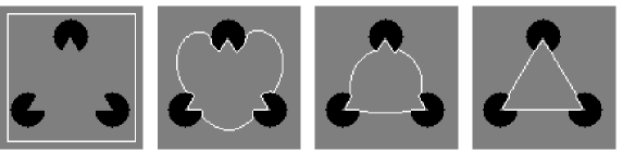
Figure 11: Kanizsa’ illusory triangle as a stable local minimum to the proposed contour energy.

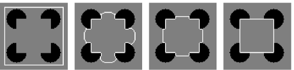
Figure 12: Kanizsa’ illusory square as a stable local minimum and the stagnation process.

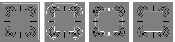
Figure 13: An illusory square emerges from a configuration of real contour bundles. The object-based supervised level-set computation works equally well for contour-based illusory contours due to the mollification operator applied to a given image $u$.

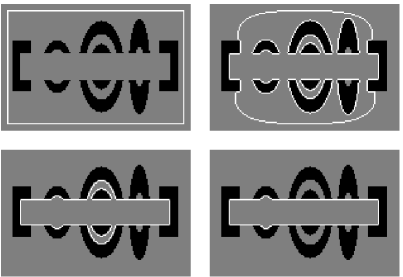
Figure 14: An illusory contour emerges from a complex configuration $Q$ of objects, as captured by the supervised level-set-based active contours. The small hump in the final output (near the left end of the illusory bar) is not due to numerical defection but to the competition between the two weights $\alpha$ and $\beta$ in the model.

Figure 15: The consequence of first-order geometric modeling: our model can efficiently capture illusory objects and contours in their first-order proximity. To achieve high order fidelity, the model should incorporate at least the curvature information, as in the earlier works of Zhu and Chan [30, 31]. Such high order models are, however, often highly challenging for both rigorous theoretical analysis and efficient numerical computation. In-depth analysis in Section 2 is often difficult to establish for high order models.

References

- [1] E. H. Adelson. Lightness perception and lightness illusions. In M. Gazzaniga, editor, The New Cognitive Neurosciences, pages 339–351. MIT press, 2nd edition, 2000.
- [2] T. F. Chan, S.-H. Kang, and J. Shen. Euler’s elastica and curvature based inpainting. SIAM J. Appl. Math., 63(2):564–592, 2002.
- [3] T. F. Chan, S. Osher, and J. Shen. The digital TV filter and nonlinear denoising. IEEE Trans. Image Process., 10(2):231–241, 2001.
- [4] T. F. Chan and J. Shen. Nontexture inpainting by curvature driven diffusions (CDD). J. Visual Comm. Image Rep., 12(4):436–449, 2001.
- [5] T. F. Chan and J. Shen. Mathematical models for local nontexture inpaintings. SIAM J. Appl. Math., 62(3):1019–1043, 2002.
- [6] T. F. Chan and J. Shen. Image Processing and Analysis: variational, PDE, wavelet, and stochastic methods. SIAM Publisher, Philadelphia, 2005.
- [7] T. F. Chan and L. A. Vese. Active contours without edges. IEEE Trans. Image Process., 10(2):266–277, 2001.
- [8] S. Esedoglu and J. Shen. Digital inpainting based on the Mumford-Shah-Euler image model. European J. Appl. Math., 13:353–370, 2002.
- [9] G. B. Folland. Real Analysis - Modern Techniques and Their Applications. John Wiley & Sons, Inc., second edition, 1999.
- [10] W. T. Freeman. The generic viewpoint assumption in a framework for visual perception. Nature, 368:542–545, 1994.
- [11] G. Kanizsa. Organization in Vision. Praeger, New York, 1979.
- [12] M. Kass, A. Witkin, and D. Terzopoulos. Snakes: active contour models. Int’l J. Comp. Vision, 1(4):321–331, 1987.
- [13] J. L. Kelley. General Topology. Springer Verlag, 1997.
- [14] D. Kersten. High-level vision and statistical inference. In M. S. Gazzaniga, editor, The New Cognitive Neurosciences, pages 353–363. The MIT Press, Cambridge, MA, USA.
- [15] S. Kichenassamy, A. Kumar, P. Olver, A. Tannenbaum, and A. Yezzi. Conformal curvature flows: from phase transitions to active vision. Arch. Rational Mech. Anal., 134(3):275 301, 1996.
- [16] D. C. Knill and D. Kersten. Apparent surface curvature affects lightness perception. Nature, 351:228–230, 1991.
- [17] D. Mumford. Elastica and computer vision. In C. L. Bajaj, editor, Algebraic Geometry and its Applications, pages 491–506. Springer-Verlag, New York, 1994.
- [18] D. Mumford and J. Shah. Optimal approximations by piecewise smooth functions and associated variational problems. Comm. Pure Applied. Math., 42:577–685, 1989.
- [19] M. Nitzberg, D. Mumford, and T. Shiota. Filtering, Segmentation, and Depth. Lecture Notes in Comp. Sci., Vol. 662. Springer-Verlag, Berlin, 1993.
- [20] A. V. Oppenheim and A. S. Willsky. Signals and Systems. Prentice Hall, 1996.
- [21] S. Osher and N. Paragios. Geometric Level Set Methods in Imaging, Vision and Graphics. Springer Verlag, 2002.
- [22] S. Osher and J. A. Sethian. Fronts propagating with curvature-dependent speed: Algorithms based on Hamilton-Jacobi formulations. J. Comput. Phys., 79(12):12–49, 1988.
- [23] L. Rudin, S. Osher, and E. Fatemi. Nonlinear total variation based noise removal algorithms. Physica D, 60:259–268, 1992.
- [24] A. Sarti, R. Malladi, and J. A. Sethian. Subjective surfaces: A geometric model for boundary completion. Int’l J. Comp. Vision, 46(3):201–221, 2002.
- [25] J. A. Sethian. A marching level set method for monotonically advancing fronts. Proc. Nat. Acad. Sci., 93(4):1591–1595, 1996.
- [26] J. A. Sethian. Level Set Methods and Fast Marching Methods. Cambridge University Press, 2nd edition, 1999.
- [27] J. Shen. On the foundations of vision modeling I. Weber’s law and Weberized TV (total variation) restoration. Physica D: Nonlinear Phenomena, 175:241–251, 2003.
- [28] J. Shen. Bayesian video dejittering by BV image model. SIAM J. Appl. Math., 64(5):1691–1708, 2004.
- [29] J. Shen. On the foundations of vision modeling III. Noncommutative monoids of occlusive preimages. J. Math. Imag. Vision, in press, 2005.
- [30] W. Zhu and T. Chan. Capture illusory contours: A level set based approach. UCLA CAM Tech. Report, 03-65, 2003.
- [31] W. Zhu and T. Chan. Illusory contours using shape information. UCLA CAM Tech. Report, 03-09, 2005.