Deterministic boundary recognition and topology extraction
for large sensor networks

Abstract

We present a new framework for the crucial challenge of self-organization of a large sensor network. The basic scenario can be described as follows: Given a large swarm of immobile sensor nodes that have been scattered in a polygonal region, such as a street network. Nodes have no knowledge of size or shape of the environment or the position of other nodes. Moreover, they have no way of measuring coordinates, geometric distances to other nodes, or their direction. Their only way of interacting with other nodes is to send or to receive messages from any node that is within communication range. The objective is to develop algorithms and protocols that allow self-organization of the swarm into large-scale structures that reflect the structure of the street network, setting the stage for global routing, tracking and guiding algorithms.

Our algorithms work in two stages: boundary recognition and topology extraction. All steps are strictly deterministic, yield fast distributed algorithms, and make no assumption on the distribution of nodes in the environment, other than sufficient density.

1 Introduction

In recent time, the study of wireless sensor networks (WSN) has become a rapidly developing research area that offers fascinating perspectives for combining technical progress with new applications of distributed computing. Typical scenarios involve a large swarm of small and inexpensive processor nodes, each with limited computing and communication resources, that are distributed in some geometric region; communication is performed by wireless radio with limited range. As energy consumption is a limiting factor for the lifetime of a node, communication has to be minimized. Upon start-up, the swarm forms a decentralized and self-organizing network that surveys the region.

From an algorithmic point of view, the characteristics of a sensor network require working under a paradigm that is different from classical models of computation: absence of a central control unit, limited capabilities of nodes, and limited communication between nodes require developing new algorithmic ideas that combine methods of distributed computing and network protocols with traditional centralized network algorithms. In other words: How can we use a limited amount of strictly local information in order to achieve distributed knowledge of global network properties?

This task is much simpler if the exact location of each node is known. Computing node coordinates has received a considerable amount of attention. Unfortunately, computing exact coordinates requires the use of special location hardware like GPS, or alternatively, scanning devices, imposing physical demands on size and structure of sensor nodes. As we demonstrated in our paper [10], current methods for computing coordinates based on anchor points and distance estimates encounter serious difficulties in the presence of even small inaccuracies, which are unavoidable in practice.

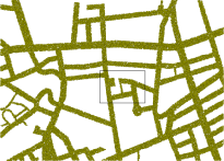
(a) 60,000 sensor nodes, uniformly distributed in a polygonal region.

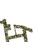
(b) A zoom into (a) shows the communication graph.

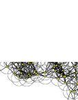
(c) A further zoom shows the communication ranges.

Figure 1: Scenario of a geometric sensor network, obtained by scattering sensor nodes in the street network surrounding Braunschweig University of Technology.

When trying to extract robust cluster structures from a huge swarm of nodes scattered in a street network of limited size, trying to obtain individual coordinates for all nodes is not only extremely difficult, but may indeed turn out to be a red-herring chase. As shown in [9], there is a way to sidestep many of the above difficulties, as some structural location aspects do not depend on coordinates. This is particularly relevant for sensor networks that are deployed in an environment with interesting geometric features. (See [9] for a more detailed discussion.) Obviously, scenarios as the one shown in Figure 1 pose a number of interesting geometric questions. Conversely, exploiting the basic fact that the communication graph of a sensor network has a number of geometric properties provides an elegant way to extract structural information.

One key aspect of location awareness is boundary recognition, making sensors close to the boundary of the surveyed region aware of their position. This is of major importance for keeping track of events entering or leaving the region, as well as for communication with the outside. More generally, any unoccupied part of the region can be considered a hole, not necessary because of voids in the geometric region, but also because of insufficient coverage, fluctuations in density, or node failure due to catastrophic events. Neglecting the existence of holes in the region may also cause problems in communication, as routing along shortest paths tends to put an increased load on nodes along boundaries, exhausting their energy supply prematurely; thus, a moderately-sized hole (caused by obstacles, by an event, or by a cluster of failed nodes) may tend to grow larger and larger. (See [7].) Therefore, it should be stressed that even though in our basic street scenario holes in the sensor network are due to holes in the filled region, our approach works in other settings as well.

Once the boundary of the swarm is obtained, it can be used as a stepping stone for extracting further structures. This is particularly appealing in our scenario, in which the polygonal region is a street network: In that scenario, we have a combination of interesting geometric features, a natural underlying structure of moderate size, as well as a large supply of practical and relevant benchmarks that are not just some random polygons, but readily available from real life. More specifically, we aim at identifying the graph in which intersections are represented by vertices, and connecting streets are represented by edges. This resulting cluster structure is perfectly suited for obtaining useful information for purposes like routing, tracking or guiding. Unlike an arbitrary tree structure that relies on the performance of individual nodes, it is robust.

Related Work:

[2] is the first paper to introduce a communication model based on quasi-unit disk graphs (QUDGs). A number of articles deal with node coordinates; most of the mathematical results are negative, even in a centralized model of computation. [3] shows that unit disk graph (UDG) recognition is NP-hard, while [1] shows NP-hardness for the more restricted setting in which all edge lengths are known. [12] shows that QUDG recognition, i.e., UDG approximation, is also hard; finally, [4] show that UDG embedding is hard, even when all angles between edges are known. The first paper (and to the best of our knowledge, the only one so far) describing an approximative UDG embedding is [13]; however, the approach is centralized and probabilistic, yielding (with high probability) a $\mathcal{O}(\log^{2.5}n\sqrt{\log\log n})$-approximation.

There are various papers dealing with heuristic localization algorithms; e.g., see [5, 6, 15, 16, 17]. In this context, see our paper [10] for an experimental study pointing out the serious deficiencies of some of the resulting coordinates.

Main Results:

Our main result is the construction of an overall framework that allows a sensor node swarm to self-organize into a well-structured network suited for performing tasks such as routing, tracking or other challenges that result from popular visions of what sensor networks will be able to do. The value of the overall framework is based on the following aspects:

• We give a distributed, deterministic approach for identifying nodes that are in the interior of the polygonal region, or near its boundary. Our algorithm is based on topological considerations and geometric packing arguments.

• Using the boundary structure, we describe a distributed, deterministic approach for extracting the street graph from the swarm. This module also uses a combination of topology and geometry.

• The resulting framework has been implemented and tested in our simulation environment Shawn; we display some experimental results at the end of the paper.

The rest of this paper is organized as follows. In the following Section 2 we describe underlying models and introduce necessary notation. Section 3 deals with boundary recognition. This forms the basis for topological clustering, described in Section 4. Section 5 describes some computational experiments with a realistic network.

2 Models and Notation

Sensor network:

A Sensor Network is modeled by a graph $G=(V,E)$, with an edge between any two nodes that can communicate with each other. For a node $v\in V$, we define $N_{k}(v)$ to be the set of all nodes that can be reached from $v$ within at most $k$ edges. The set $N(v)=N_{1}(v)$ contains the direct neighbors of $v$, i.e., all nodes $w\in V$ with $vw\in E$. For convenience we assume that $v\in N(v)$ $\forall v\in V$. For a set $U\subseteq V$, we define $N_{k}(U):=\cup_{u\in U}N_{k}(u)$. The size of the largest $k$-hop neighborhood is denoted by $\Delta_{k}:=\max_{v\in V}|N_{k}(v)|$. Notice that for geometric radio networks with even distribution, $\Delta_{k}=\mathcal{O}(k^{2}\Delta_{1})$ is a reasonable assumption.

Each node has a unique ID of size $\mathcal{O}(\log|V|)$. The identifier of a node $v$ is simply $v$.

Every node has is equipped with local memory of size $\mathcal{O}(\Delta^{2}_{\mathcal{O}(1)}\log|V|)$. Therefore, each node can store a subgraph consisting of nodes that are at most $\mathcal{O}(1)$ hops away, but not the complete network.

Computation:

Storage limitation is one of the main reasons why sensor networks require different algorithms: Because no node can store the whole network, simple algorithms that collect the full problem data at some node to perform centralized computations are infeasible.

Due to the distributed nature of algorithms, the classic means to describe runtime complexity are not sufficient. Instead, we use separate message and time complexities: The former describes the total number of messages that are sent during algorithm execution. The time complexity describes the total runtime of the algorithm over the whole network.

Both complexities depend heavily on the computational model. For our theoretical analysis, we use a variant of the well-established $\mathcal{CONGEST}$ model [14]: All nodes start their local algorithms at the same time (simultaneous wakeup). The nodes are synchronized, i.e., time runs in rounds that are the same for all nodes. In a single round, a node can perform any computation for which it has complete data. All messages arrive at the destination node at the beginning of the subsequent round, even if they have the same source or destination. There are no congestion or message loss effects. The size of a message is limited to $\mathcal{O}(\log|V|)$ bits. Notice that this does only affect the message complexity, as there is no congestion. We will use messages of larger sizes in our algorithms, knowing that they can be broken down into smaller fragments of feasible size.

Geometry:

All sensor nodes are located in the two-dimensional plane, according to some mapping $p:V\to\mathbb{R}^{2}$. It is a common assumption that the ability to communicate depends on the geometric arrangement of the nodes. There exists a large number of different models that formalize this assumption. Here we use the following reasonable model:

We say $p$ is a $d$-Quasi Unit Disk Embedding of $G$ for parameter $d\leq 1$, if both

$$uv\in E \Longrightarrow \|p(u)-p(v)\|_{2}\leq 1$$

$$uv\in E \Longleftarrow \|p(u)-p(v)\|_{2}\leq d$$

hold. $G$ itself is called a $d$-Quasi Unit Disk Graph ($d$-QUDG) if an embedding exists. A $1$-QUDG is called a Unit Disk Graph (UDG). Throughout this paper we assume that $G$ is a $d$-QUDG for some $d\geq\tfrac{1}{2}\sqrt{2}$. The reason for this particular bound lies in Lemma 3.1, which is crucial for the feasibility of our boundary recognition algorithm. The network nodes know the value of $d$, and the fact that $G$ is a $d$-QUDG. The embedding $p$ itself is not available to them.

An important property of our algorithms is that they do not require a specific distribution of the nodes. We only assume the existence of the embedding $p$.

3 Boundary Recognition

This section introduces algorithms that detect the boundary of the region that is covered by the sensor nodes. First, we present some properties of QUDGs. These allow deriving geometric knowledge from the network graph without knowing the embedding $p$. Then we define the Boundary Detection Problem, in which solutions are geometric descriptions of the network arrangement. Finally, we describe a start procedure and an augmentation procedure. Together, they form a local improvement algorithm for boundary detection.

3.1 QUDG Properties.

We start this section with a simple property of QUDGs. The special case where $d=1$ was originally proven by Breu and Kirkpatrick [3]. Recall that we assume $d\geq\sqrt{2}/2$.

Lemma 3.1

Let $u,v,w,x$ be four different nodes in $V$, where $uv\in E$ and $wx\in E$. Assume the straight-line embeddings of $uv$ and $wx$ intersect. Then at least one of the edges in $F:=\{uw,ux,vw,vx\}$ is also in $E$.

• We assume $p(u)\neq p(v)$; otherwise the lemma is trivial. Let $a:=\|p(u)-p(v)\|_{2}\leq 1$. Consider two circles of common radius $d$ with their centers at $p(u)$, resp. $p(v)$. The distance between the two intersection points of these circles is $h:=2\sqrt{d^{2}-\tfrac{1}{4}a^{2}}\geq 1$. If $F$ and $E$ were distinct, $p(w)$ and $p(x)$ had both to be outside the two circles. Because of the intersecting edge embeddings, $\|p(w)-p(x)\|_{2}>h\geq 1$, which would contradict $wx\in E$.

Lemma 3.1 allows to use edges in the graph to separate nodes in the embedding $p$, even without knowing $p$. We can use this fact to certify that a node is inside the geometric structure defined by some other nodes. Let $C\subset V$ be a chordless cycle in $G$, i.e., $(C,E(C))$ is a connected 2-regular subgraph of $G$. $P(C)$ denotes the polygon with a vertex at each $p(v),v\in C$ and an edge between vertices whose corresponding nodes are adjacent in $G$. $P(C)$ also defines a decomposition of the plane into faces. A point in the infinite face is said to be outside of $P(C)$, all other points are inside.

Corollary 3.1

Let $C$ be a chordless cycle in $G$, and let $U\subset V$ be connected. Also assume $N(C)\cap U=\varnothing$. Then either the nodes in $U$ are all on the outside of $P(C)$, or all on the inside.

This follows directly from Lemma 3.1. So we can use chordless cycles for defining cuts that separate inside from outside nodes. Our objective is to certify that a given node set is inside the cycle, thereby providing insight into the network’s geometry. Unfortunately, this is not trivial; however, it is possible to guarantee that a node set is outside the cycle.

Note that simply using two node sets that are separated by a chordless cycle $C$ and proving that the first set is outside the cycle does not guarantee that the second set is on the inside. The two sets could be on different sides of $P(C)$. So we need more complex arguments to certify insideness.

Now we present a certificate for being on the outside. Define $\mathrm{fit}_{d}(n)$ to be the maximum number of independent nodes $J$ that can be placed inside a chordless cycle $C$ of at most $n$ nodes in any $d$-QUDG embedding such that $J\cap N(C)=\varnothing$. We say that nodes are independent, if there is no edge between any two of them. These numbers exist because independent nodes are placed at least $d$ from each other, so there is a certain area needed to contain the nodes. On the other hand, $C$ defines a polygon of perimeter at most $|C|$, which cannot enclose arbitrarily large areas. Also define $\mathrm{enc}_{d}(m):=\min\{n:\mathrm{fit}_{d}(n)\geq m\}$, the minimum length needed to fit $m$ nodes.

$n$	1	2	3	4	5	6	7	8	9	10	11	12	13	14	15	16	17	18	19	20
$\mathrm{fit}_{1}(n)$	0	0	0	0	0	0	1	1	2	3	4	5	7	8	9	12	14	16	17	19
$\lim_{d\uparrow 1}\mathrm{fit}_{d}(n)$	0	0	0	0	0	1	1	2	3	4	5	7	8	9	12	14	16	17	19	23

Table 1: First values of $\mathrm{fit}_{d}(n)$

The first 20 values of $\mathrm{fit}_{1}$ and $\mathrm{fit}_{1-\varepsilon}$ for some small $\varepsilon$ are shown in Table 1. They can be obtained by considering hexagonal circle packings. Because these are constants it is reasonable to assume that the first few values of $\mathrm{fit}_{d}$ are available to every node.

We are not aware of the exact values of $\mathrm{fit}_{d}$ for all $d$. However, our algorithms just need upper bounds for $\mathrm{fit}_{d}$, and lower bounds for $\mathrm{enc}_{d}$. (An implementation of the following algorithms has to be slightly adjusted to use bounds instead of exact values.)

Now we can give a simple criterion to decide that a node set is outside a chordless cycle:

Lemma 3.2

Let $C$ be a chordless cycle and $I\subset V\setminus N(C)$ be a connected set that contains an independent subset $J\subset I$. If $|J|>\mathrm{fit}_{d}(|C|)$, then every node in $I$ is outside $P(C)$.

• By Corollary 3.1 and the definition of $\mathrm{fit}_{d}$.

3.2 Problem statement.

In this section, we define the Boundary Detection Problem. Essentially, we are looking for node sets and chordless cycles, where the former are guaranteed to be on the inside of the latter. For the node sets to become large, the cycles have to follow the perimeter of the network region. In addition, we do not want holes in the network region on the inside of the cycles, to ensure that each boundary is actually reflected by some cycle.

We now give formal definitions for these concepts. We begin with the definition of a hole: The graph $G$ and its straight-line embedding w.r.t. $p$ defines a decomposition of the plane into faces. A finite face $F$ of this decomposition is called $h$-hole with parameter $h$ if the boundary length of the convex hull of $F$ strictly exceeds $h$. An important property of an $h$-hole $F$ is the following fact: Let $C$ be a chordless cycle with $|C|\leq h$. Then all points $f\in F$ are on the outside of $P(C)$.

To describe a region in the plane, we use chordless cycles in the graph that follow the perimeter of the region. There is always one cycle for the outer perimeter. If the region has holes, there is an additional cycle for each of them. We formalize this in the opposite direction: Given the cycles, we define the region that is enclosed by them. So let $\mathcal{C}:=(C_{b})_{b\in\mathcal{B}}$ be a family of chordless cycles in the network. It describes the boundary of the region $A(\mathcal{C})\subset\mathbb{R}^{2}$, which is defined as follows. First let $\tilde{A}$ be the set of all points $x\in\mathbb{R}^{2}$ for which the cardinality of $\{b\in\mathcal{B}:x\mbox{ is on the inside of }P(C_{b})\}$ is odd. This set gives the inner points of the region, which are all points that are surrounded by an odd number of boundaries. The resulting region is defined by

(3.1) $$A(\mathcal{C}):=\bigcup_{b\in\mathcal{B}}P(C_{b})\cup\tilde{A}\;.$$

Figure 2: Area described by four boundary cycles.

See Figure 2 for an example with some cycles and the corresponding region.

We can use this approach to introduce geometry descriptions. These consist of some boundary cycles $(C_{b})_{b\in\mathcal{B}}$, and nodes sets $(I_{i})_{i\in\mathcal{I}}$ that are known to reside within the described region. The sets are used instead of direct representations of $A(\mathcal{C})$, because we seek descriptions that are completely independent of the actual embedding of the network. There is a constant $K$ that limits the size of holes. We need $K$ to be large enough to find cycles in the graph that cannot contain $K$-holes. Values $K\approx 15$ fulfill these needs.

Definition 3.1

A feasible geometry description (FGD) is a pair $(\mathcal{C},(I_{i})_{i\in\mathcal{I}})$ with $\mathcal{C}=(C_{b})_{b\in\mathcal{B}}$ of node set families that fulfills the following conditions:
(F1) Each $C_{b}$ is a chordless cycle in $G$ that does not contain any node from the family $(I_{i})_{i\in\mathcal{I}}$.
(F2) There is no edge between different cycles.
(F3) For each $v\in I_{i}$ ($i\in\mathcal{I}$), $p(v)\in A(\mathcal{C})$.
(F4) For every component $A^{\prime}$ of $A(\mathcal{C})$, there is an index $i\in\mathcal{I}$, such that $p(v)\in A^{\prime}$ $\forall v\in I_{i}$ and $p(v)\notin A^{\prime}$ $\forall v\in I_{j},j\neq i$.
(F5) $A(\mathcal{C})$ does not contain an inner point of any $k$-hole for $k>K$.

Note that condition (F4) correlates some cycles with a component of $A(\mathcal{C})$, which in turn can be identified by an index $i\in\mathcal{I}$. This index is denoted by $\mathrm{IC}(v)$, where $v\in V$ is part of such a cycle or the corresponding $I_{i}$.

See Figure 6 in the computational experience section for an example network. Figures 6 and 7 show different FGDs in this network.

We are looking for a FGD that has as many inside nodes as possible, because that forces the boundary cycles to follow the network boundary as closely as possible. The optimization problem we consider for boundary recognition is therefore

(3.2) $$\mbox{(BD)}\left\{\begin{array}[]{ll}\max&|\cup_{i\in\mathcal{I}}I_{i}|\\ \mbox{s.t.}&((C_{b})_{b\in\mathcal{B}},(I_{i})_{i\in\mathcal{I}})\mbox{ is a FGD}\end{array}\right.\;.$$

3.3 Algorithm.

We solve (BD) with local improvement methods that switch from one FGD to another of larger $|\cup_{i\in\mathcal{I}}I_{i}|$. In addition to the FGD, our algorithms maintain the following sets:

• The set $C:=\cup_{b\in\mathcal{B}}C_{b}$ of cycle nodes.

• $N(C)$, the cycle neighbors. Notice $C\subseteq N(C)$.

• $I:=\cup_{i\in\mathcal{I}}I_{i}$, the inner nodes. Our algorithms ensure $I\cap N(C)=\varnothing$ (this is no FGD requirement), and all $I_{i}$ will be connected sets. This is needed in several places for Lemma 3.2 to be applicable.

• $J\subseteq I$, consisting of so-called independent inners. These nodes form an independent set in $G$.

• the set $U:=V\setminus(N(C)\cup I)$ of unexplored nodes.

Initially, $U=V$, all other sets are empty.

We need to know how many independent nodes are in a given $I_{i}$ as proof that a cycle cannot accidently surround $I_{i}$. Because all considered cycles consist of at most $K$ nodes, every count exceeding $\mathrm{fit}_{d}(K)$ has the same implications. So we measure the mass of an $I_{i}$ by

(3.3) $$M(i):=\min\{|J\cap I_{i}|,\mathrm{fit}_{d}(K)+1\}\;.$$

Because we are interested in distributed algorithms, we have to consider what information is available at the individual nodes. Our methods ensure (and require) that each node knows to which of the above sets it belongs. In addition, each cycle node $v\in C$ knows $\mathrm{IC}(v)$, $M(\mathrm{IC}(v))$, and $N(v)\cap C$, and each cycle neighbor $w\in N(C)$ knows $N(w)\cap C$.

The two procedures are described in the following two sections: First is an algorithm that produces start solutions, second an augmentation method that increases the number of inside nodes.

3.4 Flowers.

So far, we have presented criteria by which one can decide that some nodes are outside a chordless cycle, based on a packing argument. Such a criterion will not work for the inside, as any set of nodes that fit in the inside can also be accomodated by the unbounded outside. Instead, we now present a stronger strcutural criterion that is based on a particular subgraph, an $m$-flower. For such a structure, we can prove that there are some nodes on the inside of a chordless cycle. Our methods start by searching for flowers, leading to a FGD. We begin by actually defining a flower, see Figure 4 for a visualization.

Figure 3: A 5-flower.

Figure 4: Construction of a 4-flower in a dense region.

Definition 3.2

An $m$-flower in $G$ is an induced subgraph whose node set consists of a seed $f_{0}\in V$, independent nodes $f_{1,1},\ldots,f_{1,m}\in V$, bridges $f_{2,1},\ldots,f_{2,m}\in V$, hooks $f_{3,1},\ldots,f_{3,m}\in V$, and chordless paths $W_{1},\ldots,W_{m}$, where each $W_{i}=(w_{j,1},\ldots,w_{j,\ell_{j}})\subset V$. All of these $1+3m+\sum_{j=1}^{m}\ell_{j}$ nodes have to be different nodes. For convenience, we define $f_{j,0}:=f_{j,m}$ and $f_{j,m+1}:=f_{j,1}$ for $j=1,2,3$.

The edges of the subgraph are the following: The seed $f_{0}$ is adjacent to all independent nodes: $f_{0}f_{1,j}\in E$ for $j=1,\ldots,m$. Each independent node $f_{1,j}$ is connected to two bridges: $f_{1,j}f_{2,j}\in E$ and $f_{1,j}f_{2,j+1}\in E$. The bridges connect to the hooks: $f_{2,j}f_{3,j}\in E$ for $j=1,\ldots,m$. Each path $W_{j}$ connects two hooks, that is, $f_{3,j}w_{j,1},w_{j,1}w_{j,2},\ldots,w_{j,\ell_{j}}f_{3,j+1}$ are edges in $E$.

Finally, the path lengths $\ell_{j}$, $j=1,\ldots,m$ obey

(3.4) $$\mathrm{fit}_{d}(5+\ell_{j}) < m-2\;,$$

(3.5) $$\mathrm{fit}_{d}(7+\ell_{j}) < \left\lceil\frac{1}{2}\left(\sum_{k\neq i}\ell_{k}+1\right)\right\rceil\;.$$

Notice that Equations (3.4) and (3.5) can be fulfilled: for $d=1$, $m=5$ and $\ell_{1}=\ell_{2}=\ldots=\ell_{5}=3$ are feasible. This is the flower shown in Figure 4.

The beauty of flowers lies in the following fact:

Lemma 3.3

In every $d$-QUDG embedding of a $m$-flower, the independent nodes are placed on the inside of $P(C)$, where $C:=\{f_{3,1},\ldots,f_{3,m}\}\cup\bigcup_{j=1}^{m}W_{j}$ is a chordless cycle.

• Let $P_{j}:=(f_{1,j},f_{2,j},f_{3,j},W_{j},f_{3,j+1},f_{2,j+1})$ be a petal of the flower. $P_{j}$ defines a cycle of length $5+\ell_{j}$. The other nodes of the flower are connected and contain $m-2$ independent bridges. According to (3.4), this structure is on the outside of $P(P_{j})$.

  Therefore, the petals form a ring of connected cycles, with the seed on either the inside or the outside of the structure. Assume the seed is on the outside. Consider the infinite face of the straight-line embedding of the flower. The seed is part of the outer cycle, which consists of $7+\ell_{j}$ nodes for some $j\in\{1,\ldots,m\}$. This cycle has to contain the remaining flower nodes, which contradicts  (3.5). Therefore, the seed is on the inside, and the claim follows.

Because we do not assume a particular distribution of the nodes, we cannot be sure that there is a flower in the network. Intuitively, this is quite clear, as any node may be close to the boundary, so that there are no interior nodes; as the nodes can only make use of the local graph structure, and have no direct way of detecting region boundaries, this means that for low densities everywhere, our criterion may fail. As we show in the following, we can show the existence of a flower if there is a densely populated region somewhere: We say $G$ is locally $\varepsilon$-dense in a region $A\subset\mathbb{R}^{2}$, if every $\varepsilon$-ball in $A$ contains at least one node, i.e., $\forall z\in\mathbb{R}^{2}:B_{\varepsilon}(z)\subset A\Rightarrow\exists v\in V:\|p(v)-z\|_{2}\leq\varepsilon$.

Lemma 3.4

Let $0<\varepsilon<\tfrac{3}{2}-\sqrt{2}\approx 0.086$. Assume $d=1$. If $G$ is $\varepsilon$-dense on the disk $B_{3}(z)$ for some $z\in\mathbb{R}^{2}$, then $G$ contains a $4$-flower.

• Let $w:=2(\sqrt{2}-1)$. See Figure 4. Place an $\varepsilon$-ball at all the indicated places and choose a node in each. Then the induced subgraph will contain precisely the drawn edges. Then $m=4$ and $\ell_{1}=\ldots=\ell_{4}=3$, so for $d=1$, these $\ell$-numbers are feasible.

Now we present the actual algorithm to detect flowers. Notice that a flower is a strictly local structure, so we use a very simple kind of algorithm. Each node $v\in V$ performs the following phases after the simultaneous wakeup:

1. Collect the subgraph on $N_{8}(v)$.
2. Find a flower.
3. Announce update.
4. Update.

Collect:

First, each node $v\in V$ collects and stores the local neighborhood graph $N_{8}(v)$. This can be done in time $\mathcal{O}(\Delta_{1})$ and message complexity $\mathcal{O}(\Delta_{1}\Delta_{8})$, if every nodes broadcasts its direct neighborhood to its 8-neighborhood.

Find Flower:

Then, every node decides for itself whether it is the seed of a flower. This does not involve any communication.

Announce update:

Because there could be multiple intersecting flowers, the final manifestation of flowers has to be scheduled: Every seed of some flower broadcasts an announcement to all nodes of the flower and their neighbors. Nodes that receive multiple announcements decide which seed has higher priority, e.g., higher ID number. The seeds are then informed whether they lost such a tie-break. This procedure has runtime $\mathcal{O}(1)$ and message complexity $\mathcal{O}(\Delta_{9})$ per seed, giving a total message complexity of $\mathcal{O}(\Delta_{9}|V|)$.

Update:

The winning seeds now inform their flowers that the announced updates can take place. This is done in the same manner as the announcements. The nodes that are part of a flower store their new status and the additional information described in Section 3.3.

3.5 Augmenting Cycles.

Now that we have an algorithm to construct an initial FGD in the network, we seek an improvement method. For that, we employ augmenting cycles. Consider an FGD $((C_{b})_{b\in\mathcal{B}},(I_{i})_{i\in\mathcal{I}})$. Let $U=(u_{1},u_{2},\ldots,u_{|U|})\subset V$ be a (not necessarily chordless) cycle. For convenience, define $u_{0}:=u_{|U|}$ and $u_{|U|+1}:=u_{1}$.

When augmenting, we open the cycles $(C_{b})_{b\in\mathcal{B}}$ where they follow $U$, and reconnect the ends according to $U$. Let $U^{-}:=\{u_{i}\in U:u_{i-1},u_{i},u_{i+1}\in C\}$ and $U^{+}:=U\setminus C$. The resulting cycle nodes of the augmentation operation are then $C^{\prime}:=C\cup U^{+}\setminus U^{-}$. If $N(U)\cap I=\varnothing$, this will not affect inside nodes, and it may open some new space for the inside nodes to discover. In addition, as the new cycle cannot contain a $|U|$-hole, we can limit $|U|$ to guarantee condition (F5).

We use a method that will search for an augmenting cycle that will lead to another FGD with a larger number of inside nodes, thereby performing one improvement step. The method is described for a single node $v_{1}\in C$ that searches for an augmenting cycle containing itself. This node is called initiator of the search.

It runs in the following phases:

1. Cycle search.
2. Check solution.
(a) Backtrack.
(b) Query feasibility.
3. Announce update.
4. Update.

Cycle search:

$v_{1}$ initiates the search by passing around a token. It begins with the token $T=(v_{1})$. Each node that receives this token adds itself to the end of it and forwards it to a neighbor. When the token returns from there, the node forwards it to the next feasible neighbor. If there are no more neighbors, the node removes itself from the list end and returns the token to its predecessor.

The feasible neighbors to which $T$ gets forwarded are all nodes in $V\setminus I$. The only node that may appear twice in the token is $v_{1}$, which starts the “check solution” phase upon reception of the token. In addition, $T$ must not contain a cycle node between two cycle neighbors. The token is limited to contain

(3.6) $$|T| < \min_{v\in T\cap C}\mathrm{enc}_{d}(M(\mathrm{IC}(v)))$$

(3.7) $$\leq K$$

nodes. This phase can be implemented such that no node (except for $v_{1}$) has to store any information about the search. When this phase terminates unsuccessfully, i.e., without an identified augmenting cycle, the initiator exits the algorithm.

Check Solution:

When the token gets forwarded to $v_{1}$, it describes a cycle. $v_{1}$ then sends a backtrack message backwards along $T$:

Backtrack:

While the token travels backwards, each node performs the following: If it is a cycle node, it broadcasts a query containing $T$ to its neighbors, which in turn respond whether they would become inside nodes after the update. Such nodes are called new inners. Then, the cycle node stores the number of positive responses in the token.

A non-cycle node checks whether it would have any chords after the update. In that case, it cancels the backtrack phase and informs $v_{1}$ to continue the cycle search phase.

Query Feasibility:

When the backtrack message reaches $v_{1}$, feasibility is partially checked by previous steps. Now, $v_{1}$ checks the remaining conditions.

Let $\mathcal{I}^{\prime}:=\{\mathrm{IC}(v):v\in C\cap T\}$. First, it confirms that for every $i\in\mathcal{I}$ there is a matching cycle node in the token that has a nonzero new inner count. Then it picks a $i^{\prime}\in\mathcal{I}$. All new inners of cycle nodes of this $\mathrm{IC}$ value then explore the new inner region that will exist after the update. This can be done by a BFS that carries the token. The nodes report back to $v_{1}$ the $\mathrm{IC}$ values of new inner nodes that could be reached. If this reported set equals $\mathcal{I}^{\prime}$, $T$ is a feasible candidate for an update and phase “announce update” begins. Otherwise, the cycle search phase continues.

Announce update:

Now $T$ contains a feasible augmenting cycle. $v_{1}$ informs all involved nodes that an update is coming up. These nodes are $T$, $N(T)$ and all nodes that can be reached from any new inner in the new region. This is done by a distributed BFS as in the “query feasibility” phase. Let $I^{\prime}$ be the set of all nodes that will become inner nodes after the update. During this step, the set $J$ of independent nodes is also extended in a simple greedy fashion.

If any node receives multiple update announcements, the initiator node of higher ID wins. The loser is then informed that its announcement failed.

Update:

When the announcement successfully reached all nodes without losing a tie-break somewhere, the update is performed.

If there is just one component involved, i.e., $|\mathcal{I}^{\prime}|=1$, the update can take place immediatly.

If $|\mathcal{I}^{\prime}|>1$, there might be problems keeping $M(\mathrm{IC}(\cdot))$ accurate if multiple augmentations happen simultaneously. So $v_{1}$ first decides that the new ID of the merged component will be $v_{1}$. It then determines what value $M(\mathrm{IC}(v_{1}))$ will take after the update. If this value strictly exceeds $\mathrm{fit}_{d}(K)$, $M(\mathrm{IC}(v_{1}))$ is independent of potential other updates; the update can take place immediately. However, $M(\mathrm{IC}(v_{1}))\leq\mathrm{fit}_{d}(K)$, concurrent updates have to be schedules. So $v_{1}$ floods the involved components with an update announcement, and performs its update after all others of higher prioity, i.e., higher initiator ID.

Finally, all nodes in $T$ flood their $\tfrac{K}{2}$-hop neighborhood so that cycle nodes whose cycle search phase was unsuccessful can start a new attempt, because their search space has changed.

Lemma 3.5

If the augmenting cycle algorithm performs an update on a FGD, it produces another FGD with strictly more inner nodes.

• We need to show that all five FGD conditions are met: (F1) and (F2) are checked in the backtrack phase, (F3) follows from (3.6), (F4) from the connectivity test in the feasibility check phase, and (F5) follows from (3.7). The increase in inner nodes is assured in the query feasibility phase.

Lemma 3.6

One iteration of the augmenting cycle algorithm for a given initiator nodes has message complexity $\mathcal{O}(\Delta_{K}^{K}|V|)$ and time complexity $\mathcal{O}(\Delta_{K}^{K}\Delta_{1}+|V|)$.

• There at at most $\Delta_{K}^{K}$ cycles that are checked. For one cycle, the backtrack phase takes $\mathcal{O}(\Delta_{1})$ message and time complexity. The query feasibility phase involves flooding the part of the new inside that is contained in the cycle. Because there can be any number of nodes in this region, message complexity for this flood is $\mathcal{O}(|V|)$. The flood will be finished after at most $2\mathrm{fit}_{d}(K)$ communication rounds, the time complexity is therefore $\mathcal{O}(1)$. After a feasible cycle was found, the announce update and update phases happen once. Both involve a constant number of floods over the network, their message and time complexities are therefore $\mathcal{O}(|V|)$. Combining these complexities results in the claimed values.

4 Topological Clustering

This section deals with constructing clusters that follow the geometric network topology. We use the working boundary detection from the previous section and add a method for clustering.

4.1 Problem statement.

We assume the boundary cycle nodes are numbered, i.e., $C_{b}=(c_{b,1},\ldots,c_{b,|C_{b}|})$ for $b\in\mathcal{B}$. We use a measure $\tilde{d}$ that describes the distance of nodes in the subgraph $(C,E(C))$:

$$\tilde{d}(c_{b,j},c_{b^{\prime},j^{\prime}}):=\left\{\begin{array}[]{cl}+\infty&\!\!\!\mbox{if }b\neq b^{\prime}\\ \min\{|j^{\prime}-j|,|C_{b}|-|j^{\prime}-j|\}&\!\!\!\mbox{if }b=b^{\prime}\end{array}\right.$$

That is, $\tilde{d}$ assigns nodes on the same boundary their distance within this boundary, and $\infty$ to nodes on different boundaries.

For each node $v\in V$, let $Q_{v}\in C$ be the set of cycle nodes that have minimal hop-distance to $v$, and let $s_{v}$ be this distance. These nodes are called anchors of $v$. Let $v\in V$ and $u,w\in N(v)$. We say $u$ and $w$ have distant anchors w.r.t. $v$, if there are $q_{u}\in Q_{u}$ and $q_{v}\in Q_{v}$ such that $\tilde{d}(q_{u},q_{w})>\pi(s_{v}+1)$ holds (with $\pi=3.14\ldots$). This generalizes closeness to multiple boundaries to the closeness to two separate pieces of the same boundary. (Here “separate pieces” means that there is sufficient distance along the boundary between the nodes to form a half-circle around $v$.)

$v$ is called $k$-Voronoi node, if $N(v)$ contains at least $k$ nodes with pairwise distant anchors. We use these nodes to identify nodes that are precisely in the middle between some boundaries. Let $V_{k}$ be the set of all $k$-Voronoi nodes. Our methods are based on the observation that $V_{2}$ forms strips that run between two boundaries, and $V_{3}$ contains nodes where these strips meet.

The connected components of $V_{3}$ are called intersection cores. We build intersection clusters around them that extend to the boundary. The remaining strips are the base for street clusters connecting the intersections.

4.2 Algorithms.

We use the following algorithm for the clustering:
1. Synchronize end of boundary detection.
2. Label boundaries.
3. Identify intersection cores.
4. Cluster intersections and streets.

Synchronize:

The second phase needs to be started at all cycle nodes simultaneously, after the boundary detection terminates. For that matter, we use a synchronization tree in the network, i.e., a spanning tree. Every node in the tree keeps track of whether there are any active initiator nodes in their subtree. When the synchronization tree root detects that there are no more initiators, it informs the cycle nodes to start the second phase. Because the root knows the tree depth, it can ensure the second phase starts in sync.

Label:

Now the cycle nodes assign themselves consecutive numbers. Within each cycle $C_{b}$, this starts at the initiator node of the last augmentation step. If $C_{b}$ stems from a flower that has not been augmented, some node that has been chosen by the flower’s seed takes this role. This start node becomes $c_{b,1}$. It then sends a message around the cycle so that each node knows its position. Afterwards, it sends another message with the total number of nodes in the cycle. In the end, each node $c_{b,j}$ knows $b$, $j$, and $|C_{b}|$. Finally, the root of the synchronization tree gets informed about the completion of this phase.

Intersection cores:

This phase identifies the intersection cores. It starts simultaneously at all cycle nodes. This is scheduled via the synchronization tree. This tree’s root knows the tree depth. Therefore, it can define a start time for this phase and broadcast a message over the tree that reaches all nodes shortly before this time. Then the cycle nodes start a BFS so that every node $v$ knows one $q_{v}\in Q_{v}$ and $s_{v}$. The BFS carries information about the anchors so that $v$ also knows $b$ and $j$ for which $q_{v}=c_{b,j}$. Also, each nodes stores this information for all of its neighbors.

Each node $v$ checks whether there are three nodes $u_{1},u_{2},u_{3}\in N(v)$ whose known anchors are distant, i.e., $\tilde{d}(q_{u_{j}},q_{u_{k}})>\pi(s_{v}+1)$ for $j\neq k$. In that case, $v$ declares itself to be a 3-Voronoi node. This constructs a set $\tilde{V}_{3}\subseteq V_{3}$.

Finally, the nodes in $\tilde{V}_{3}$ determine their connected components and the maximal value of $s_{v}$ within each component by constructing a tree within each component, and assign each component an unique ID number.

Cluster:

Now each intersection core starts BFS up to the chosen depth. Each node receiving a BFS message associates with the closest intersection core. This constructs the intersection clusters. Afterwards, the remaining nodes determine their connected components by constructing a tree within each component, thereby forming street clusters.

Because the synchronization phase runs in parallel to the boundary detection algorithm, it makes sense to analyze the runtime behaviour of this phase separately:

Theorem 4.1

The synchronization phase of the algorithm has both message and time complexity $\mathcal{O}(|V|^{3})$.

• We do not separate between time and message complexity, because here they are the same. Constructing the tree takes $\mathcal{O}(|V|\log|V|)$, and the final flood is linear. However, keeping track of the initiators is more complex: There can be $\mathcal{O}(|V|)$ augmentation steps. In each step, $\mathcal{O}(|V|)$ may change their status, which has to be broadcast over $\mathcal{O}(|V|)$ nodes.

Theorem 4.2

The remaining phases have message and time complexity $\mathcal{O}(|V|\log|V|)$.

• The most expensive operation in any of the phases is a BFS over the whole network, which takes $\mathcal{O}(|V|\log|V|)$.

5 Computational Experience

We have implemented and tested our methods with our large-scale network simulator Shawn [11]. We demonstrate the performance on a complex scenario, shown in Figure 6: The network consists of 60,000 nodes that are scattered over a street map. To show that the procedures do not require a nice distribution, we included fuzzy boundaries and varying densities. Notice that this network is in fact very sparse: The average neighborhood size is approximatly 20 in the lightly populated and 30 in the heavily populated area.

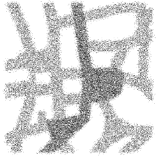
Figure 5: Example network.

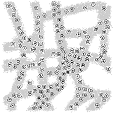
Figure 6: Boundary cycles and inside nodes identified by the flower procedure.

Figure 6 shows the FGD that is produced by the flower procedure. It includes about 70 flowers, where a single one would suffice to start the augmentation. Figure 7 shows some snapshots of the augmenting cycle method and its final state. In the beginning, many extensions to single cycles lead to growing zones. In the end, they get merged together by multi-cycle augmentations. It is obvious that the final state indeed consists of a FGD that describes the real network boundaries well.

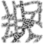
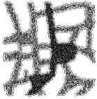
Figure 7: Two snapshots and final state of the Augmenting Cycle algorithm.

Figure 8 shows the Voronoi sets $V_{2}$ and $V_{3}$. One can clearly see the strips running between the boundaries and the intersection cluster cores that are in the middle of intersections. Finally, Figure 9 shows the clustering that is computed by our method. It consists of the intersection clusters around the 3-Voronois, and street clusters in the remaining parts. The geometric shape of the network area is reflected very closely, even though the network had no access to geometric information.

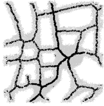
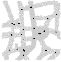
Figure 8: Identified 2-Voronoi and 3-Voronoi nodes.

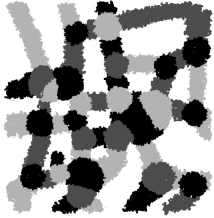
Figure 9: The final clustering.

6 Conclusions

In this paper we have described an integrated framework for the deterministic self-organization of a large swarm of sensor nodes. Our approach makes very few assumptions and is guaranteed to produce correct results; the price is dealing with relatively complex combinatorial structures such as flowers. Obviously, stronger assumptions on the network properties, the boundary structure or the distribution of nodes allow faster and simpler boundary recognition; see our papers [8] and [9] for probabilistic ideas.

Our framework can be seen as a first step towards robust routing, tracking and guiding algorithms. We are currently working on extending our framework in this direction.

References

- [1] J. Aspnes, D. Goldenberg, and Y. Yang. On the computational complexity of sensor network localization. In ALGOSENSORS, volume 3121 of LNCS. Springer, 2004.
- [2] L. Barrière, P. Fraigniaud, and L. Narayanan. Robust position-based routing in wireless ad hoc networks with unstable transmission ranges. In DIALM ’01, pages 19–27, New York, NY, USA, 2001. ACM Press.
- [3] H. Breu and D. Kirkpatrick. Unit disk graph recognition is NP-hard. Comp. Geom.: Theory Appl., 9(1-2):3–24, 1998.
- [4] J. Bruck, J. Gao, and A. A. Jiang. Localization and routing in sensor networks by local angle information. In Proc. of the 6th ACM Int. Symp. on Mobile Ad Hoc Networking and Computing (MOBIHOC), 2005.
- [5] S. Čapkun, M. Hamdi, and J. Hubaux. GPS-free positioning in mobile ad-hoc networks. In Proc. IEEE HICSS-34—vol.9, page 9008, 2001.
- [6] L. Doherty, K. Pister, and L. E. Ghaoui. Convex position estimation in wireless sensor networks. In Proc. IEEE Infocom ’01, pages 1655–1663, 2001.
- [7] Q. Fang, J. Gao, and L. Guibas. Locating and bypassing routing holes in sensor networks. In Proc. InfoCom, volume 23. IEEE, 2004.
- [8] S. Fekete, M. Kaufmann, A. Kröller, and K. Lehmann. A new approach for boundary recognition in geometric sensor networks. In Proceedings 17th Canadian Conference on Computational Geometry, 2005. (To appear).
- [9] S. P. Fekete, A. Kröller, D. Pfisterer, S. Fischer, and C. Buschmann. Neighborhood-based topology recognition in sensor networks. In ALGOSENSORS, volume 3121 of Lecture Notes in Computer Science, pages 123–136. Springer, 2004.
- [10] A. Kröller, S. P. Fekete, D. Pfisterer, S. Fischer, and C. Buschmann. Koordinatenfreies lokationsbewusstsein. Information Technology, 47:70–78, 2005.
- [11] A. Kröller, D. Pfisterer, C. Buschmann, S. P. Fekete, and S. Fischer. Shawn: A new approach to simulating wireless sensor networks. In Proceedings Design, Analysis, and Simulation of Distributed Systems (DASD05), pages 117–124, 2005.
- [12] F. Kuhn, T. Moscibroda, and R. Wattenhofer. Unit disk graph approximation. In DIALM-POMC ’04, pages 17–23, New York, NY, USA, 2004. ACM Press.
- [13] T. Moscibroda, R. O’Dell, M. Wattenhofer, and R. Wattenhofer. Virtual coordinates for ad hoc and sensor networks. In DIALM-POMC ’04, pages 8–16, New York, NY, USA, 2004. ACM Press.
- [14] D. Peleg. Distributed computing: a locality-sensitive approach. Society for Industrial and Applied Mathematics, Philadelphia, PA, USA, 2000.
- [15] N. Priyantha, H. Balakrishnan, E. Demaine, and S. Teller. Anchor-free distributed localization in sensor networks. Technical Report MIT-LCS-TR-892, MIT Laboratory for Computer Science, APR 2003.
- [16] C. Savarese, J. Rabaey, and K. Langendoen. Robust positioning algorithms for distributed ad-hoc wireless sensor networks. In Proc. 2002 USENIX Ann. Tech. Conf., pages 317–327, 2002.
- [17] N. Sundaram and P. Ramanathan. Connectivity-based location estimation scheme for wireless ad hoc networks. In Proc. IEEE Globecom ’02, volume 1, pages 143–147, 2002.