A Near Maximum Likelihood Decoding Algorithm for MIMO Systems Based on Semi-Definite Programming

Abstract

In Multi-Input Multi-Output (MIMO) systems, Maximum-Likelihood (ML) decoding is equivalent to finding the closest lattice point in an $N$-dimensional complex space. In general, this problem is known to be NP hard. In this paper, we propose a quasi-maximum likelihood algorithm based on Semi-Definite Programming (SDP). We introduce several SDP relaxation models for MIMO systems, with increasing complexity. We use interior-point methods for solving the models and obtain a near-ML performance with polynomial computational complexity. Lattice basis reduction is applied to further reduce the computational complexity of solving these models. The proposed relaxation models are also used for soft output decoding in MIMO systems.

I Introduction

Recently, there has been a considerable interest in Multi-Input Multi-Output (MIMO) antenna systems due to achieving a very high capacity as compared to single-antenna systems [4, 5]. In MIMO systems, a vector is transmitted by the transmit antennas. In the receiver, a corrupted version of this vector affected by the channel noise and fading is received. Decoding concerns the operation of recovering the transmitted vector from the received signal. This problem is usually expressed in terms of “lattice decoding” which is known to be NP-hard.

To overcome the complexity issue, a variety of sub-optimum polynomial time algorithms are suggested in the literature for lattice decoding. However, unfortunately, these algorithms usually result in a noticeable degradation in the performance. Examples of such polynomial time algorithms include: Zero Forcing Detector (ZFD) [6, 7], Minimum Mean Squared Error Detector (MMSED) [8, 9], Decision Feedback Detector (DFD) and Vertical Bell Laboratories Layered Space-Time Nulling and Cancellation Detector (VBLAST Detector) [10, 11].

Lattice basis reduction has been applied as a pre-processing step in sub-optimum decoding algorithms to reduce the complexity and achieve a better performance. Minkowski reduction [12], Korkin-Zolotarev reduction [13] and LLL reduction [14] have been successfully used for this purpose in [15, 16, 17, 18, 19, 20].

In the last decade, Sphere Decoder (SD) is introduced as a Maximum Likelihood (ML) decoding method for MIMO systems with near-optimal performance [23]. In the SD method, the lattice points inside a hyper-sphere are generated and the closest lattice point to the received signal is determined. The average complexity of this algorithm is shown to be polynomial time (almost cubic) over certain ranges of rate, Signal to Noise Ratio (SNR) and dimension, while the worst case complexity is still exponential [15, 24, 25]. However, recently, it has been shown that it is a misconception that the expected number of operations in SD asymptotically grows as a polynomial function of the problem size [26] (reference [26] derives an exponential lower bound on the average complexity of SD).

In [27], a quasi-maximum likelihood method for lattice decoding is introduced. Each signal constellation is expressed by its binary representation and the decoding is transformed into a quadratic minimization problem [27]. Then, the resulting problem is solved using a relaxation for rank-one matrices in Semi-Definite Programming (SDP) context. It is shown that this method has a near optimum performance and a polynomial time worst case complexity. However, the method proposed in [27] is limited to scenarios that the constellation points are expressed as a linear combination of bit labels. A typical example is the case of natural labeling in conjunction with PSK constellation. This restriction is removed in this work. Therefore, we are able to handle any form of constellation for an arbitrary labeling of points, for example PAM constellation with Gray labeling. Another quasi-maximum likelihood decoding method is introduced in [29] for larger PSK constellations with near ML performance and low complexity.

Recently, we became aware of another quasi-maximum likelihood decoding method [30] for the MIMO systems employing 16-QAM. They replace any finite constellation by a polynomial constraint, e.g. if $x\in\{a,b,c\}$, then $(x-a)(x-b)(x-c)=0$. Then, by introducing some slack variables, the constraints are expressed in terms of quadratic polynomials. Finally, the SDP relaxation is resulted by dropping the rank-one constraint. The work in [30] , in its current form, is restricted to MIMO systems employing 16-QAM. However, it can be generalized for larger constellations at the cost of defining more slack variables, increasing the complexity, and significantly decreasing the performance.

In this work, we develop an efficient approximate ML decoder for MIMO systems based on SDP. In the proposed method, the transmitted vector is expanded as a linear combination (with zero-one coefficients) of all the possible constellation points in each dimension. Using this formulation, the distance minimization in Euclidean space is expressed in terms of a binary quadratic minimization problem. The minimization of this problem is over the set of all binary rank-one matrices with column sums equal to one. In order to solve this minimization problem, we present two relaxation models (Model III and IV), providing a trade-off between the computational complexity and the performance (both models can be solved with polynomial-time complexity). Two additional relaxation models (Model I and II) are presented as intermediate steps in the derivations of Model III and IV.

Model I: A preliminary SDP relaxation of the minimization problem is obtained by removing the rank-one constraint in the problem and using Lagrangian duality [31]. This relaxation has many redundant constraints and no strict interior point in the feasible set (there are numerical difficulties in computing the solution for a problem without an interior point).

Model II: To overcome this drawback, the feasible set is projected onto a face of the semi-definite cone. Then, based on the identified redundant constraints, another form of the relaxation is obtained, which can be solved using interior-point methods.

Model III: The relaxation Model II results in a weak lower bound. To strengthen this relaxation model, the structure of the feasible set is investigated. An interesting property of the feasible set imposes a zero pattern for the solution. Adding this pattern as an extra constraint to the previous relaxation model results in a stronger model.

Model IV: Finally, the strongest relaxation model in this work is introduced by adding some additional non-negativity constraints. The number of non-negativity constraints can be adjusted to provide a trade-off between the performance and complexity of the resulting method.

Simulation results show that the performance of the last model is near optimal for M-ary QAM or PSK constellation (with an arbitrary binary labeling, say Gray labeling). Therefore, the decoding algorithm built on this model has a near-ML performance with polynomial computational complexity.

The proposed models result in a solution that is not necessarily a binary rank-one matrix. This solution is changed to a binary rank-one matrix through a randomization algorithm. We modify the conventional randomization algorithms to adopt to our problem. Also, a new randomization procedure is introduced which finds the optimal binary rank-one solution in a smaller number of iterations than the conventional ones. Finally, we discuss using a lattice basis reduction method to further reduce the computational complexity of the proposed relaxation models. The extension of the decoding technique for soft output decoding is also investigated.

Following notations are used in the sequel. The space of $K\times N$ (resp. $N\times N$) real matrices is denoted by ${\mathcal{M}}_{K\times N}$ (resp. ${\mathcal{M}}_{N}$), and the space of $N\times N$ symmetric matrices is denoted by ${\mathcal{S}}_{N}$. The indexing of the matrix elements start from one, unless in cases that an extra row (or column) is inserted in the first row (or column) of a matrix in which case indexing starts from zero. For a $K\times N$ matrix $\mathbf{X}\in{\mathcal{M}}_{K\times N}$ the $(i,j)$th element is represented by $x_{ij}$, where $1\leq i\leq K,\;1\leq j\leq N$, i.e. ${\bf X}=[x_{ij}]$. We use ${{\rm trace}}(\mathbf{A})$ to denote the trace of a square matrix ${\bf A}$. The space of symmetric matrices is considered with the trace inner product $\langle\mathbf{A},\mathbf{B}\rangle={{\rm trace}}(\mathbf{AB})$. For $\mathbf{A},\mathbf{B}\in{\mathcal{S}}_{N}$, $\mathbf{A}\succeq 0$ (resp. $\mathbf{A}\succ 0$) denotes positive semi-definiteness (resp. positive definiteness), and $\mathbf{A}\succeq\mathbf{B}$ denotes $\mathbf{A}-\mathbf{B}\succeq 0$. For two matrices $\mathbf{A},\mathbf{B}\in{\mathcal{M}}_{N}$, $\mathbf{A}\geq\mathbf{B}$, ($\mathbf{A}>\mathbf{B}$) means $a_{ij}\geq b_{ij}$, $(a_{ij}>b_{ij})$ for all $i,j$. The Kronecker product of two matrices $\mathbf{A}$ and $\mathbf{B}$ is denoted by $\mathbf{A}\otimes\mathbf{B}$ (for definition see [32]).

For $\mathbf{X}\in{\mathcal{M}}_{K\times N}$, ${\rm vec}(\mathbf{X})$ denotes the vector in $\mathbb{R}^{KN}$ (real $KN$-dimensional space) that is formed from the columns of the matrix $\mathbf{X}$. The following identity relates the Kronecker product with ${\rm vec}(\cdot)$ operator, see e. g. [32],

$${\rm vec}(\mathbf{ACB})=(\mathbf{B}^{T}\otimes\mathbf{A}){\rm vec}(\mathbf{C}).$$ (1)

For $\mathbf{X}\in{\mathcal{M}}_{N}$, ${\rm diag}(\mathbf{X})$ is a vector of the diagonal elements of $\mathbf{X}$. We use $\mathbf{e}_{N}\in\mathbb{R}^{N}$ (resp. $\mathbf{0}_{N}\in\mathbb{R}^{N}$) to denote the $N\times 1$ vector of all ones (resp. all zeros), $\mathbf{E}_{K\times N}\in{\mathcal{M}}_{K\times N}$ to denote the matrix of all ones, and $\mathbf{I}_{N}$ to denote the $N\times N$ Identity matrix. For $\mathbf{X}\in{\mathcal{M}}_{K\times N}$, the notation $\mathbf{X}(1:i,1:j)$, $i<k$ and $j<n$ denotes the sub-matrix of $\mathbf{X}$ containing the first $i$ rows and the first $j$ columns.

The rest of the paper is organized as follows. The problem formulation is introduced in Section II. Section III is devoted to the semi-definite solution of this problem. In Section IV, randomization procedures for finding rank-one solutions are presented. Section V introduces a method based on lattice basis reduction to reduce the computational complexity of the proposed relaxation models. In Section VI, the soft decoding methods based on the proposed models are investigated. Simulation results are presented in Section VII. Finally, Section VIII concludes the paper.

II Problem Formulation

A MIMO system with $\tilde{N}$ transmit antennas and $\tilde{M}$ receive antennas is modelled as

$$\tilde{\mathbf{y}}=\sqrt{\dfrac{S\!N\!R}{\tilde{M}\tilde{E}_{s_{av}}}}\tilde{\mathbf{H}}\tilde{\mathbf{x}}+\tilde{\mathbf{n}},$$ (2)

where $\tilde{\mathbf{H}}=\left[\tilde{h}_{ij}\right]$ is the $\tilde{M}\times\tilde{N}$ channel matrix composed of independent, identically distributed complex Gaussian random elements with zero mean and unit variance, $\tilde{\mathbf{n}}$ is an $\tilde{M}\times 1$ complex additive white Gaussian noise vector with zero mean and unit variance, and $\tilde{\mathbf{x}}$ is an $\tilde{N}\times 1$ data vector whose components are selected from a complex set $\tilde{\mathcal{S}}=\left\{\tilde{s}_{1},\tilde{s}_{2},\cdots,\tilde{s}_{K}\right\}$ with an average energy of $\tilde{E}_{s_{av}}$. The parameter $S\!N\!R$ in (2) is the SNR per receive antenna.

Noting $\tilde{x}_{i}\in\tilde{\mathcal{S}}$, for $i=1,\cdots,\tilde{N}$, we have

$$\tilde{x}_{i}=u_{i}(1)\tilde{s}_{1}+u_{i}(2)\tilde{s}_{2}+\cdots+u_{i}(K)\tilde{s}_{K},$$ (3)

where

$$u_{i}(j)\in\left\{0,1\right\}\;\;{\rm and}\;\;\sum_{j=1}^{K}u_{i}(j)=1,\;\;\forall\,i=1,\cdots,\tilde{N}.$$ (4)

Let ${\bf u}=\left[\begin{array}[]{ccccccc}u_{1}(1)&\cdots&u_{1}(K)&\cdots&u_{N}(1)&\cdots&u_{N}(K)\end{array}\right]^{T}$ and $N=\tilde{N}$. Using the equations in (3) and (4), the transmitted vector is expressed as

$$\tilde{\mathbf{x}}=\tilde{\mathbf{S}}\mathbf{u},$$ (5)

where $\tilde{\mathbf{S}}={\bf I}_{N}\otimes[\tilde{s}_{1},\cdots,\tilde{s}_{K}]$ is an $N\times NK$ matrix of coefficients, and $\mathbf{u}$ is an $NK\times 1$ binary vector such that $\mathbf{A}\mathbf{u}=\mathbf{e}_{N}$, where $\mathbf{A}={\bf I}_{N}\otimes{\bf e}_{K}^{T}$. This constraint states that among each $K$ components of the binary vector ${\bf u}$, i.e. $u_{i}(1),\cdots,u_{i}(K)$, there is only one element equal to “1” and the rest are zero.

To avoid using complex matrices, the system model (2) is represented by real matrices in (12).

$$\left[\begin{tabular}[]{c}$\mathfrak{R}\left(\tilde{\mathbf{y}}\right)$\\ $\mathfrak{I}\left(\tilde{\mathbf{y}}\right)$\\ \end{tabular}\right] = \sqrt{\dfrac{SNR}{\tilde{M}\tilde{E}_{s_{av}}}}\left[\begin{tabular}[]{cc}$\mathfrak{R}\left(\tilde{\mathbf{H}}\right)$&$\mathfrak{I}\left(\tilde{\mathbf{H}}\right)$\\ $-\mathfrak{I}\left(\tilde{\mathbf{H}}\right)$&$\mathfrak{R}\left(\tilde{\mathbf{H}}\right)$\\ \end{tabular}\right]\left[\begin{tabular}[]{c}$\mathfrak{R}\left(\tilde{\mathbf{x}}\right)$\\ $\mathfrak{I}\left(\tilde{\mathbf{x}}\right)$\\ \end{tabular}\right]$$ (12)

$$+ \left[\begin{tabular}[]{c}$\mathfrak{R}\left(\tilde{\mathbf{n}}\right)$\\ $\mathfrak{I}\left(\tilde{\mathbf{n}}\right)$\\ \end{tabular}\right]$$ (15)

$$\Rightarrow\mathbf{y} = \mathbf{H}\mathbf{x}+\mathbf{n},$$ (16)

where $\mathfrak{R}(.)$ and $\mathfrak{I}(.)$ denote the real and imaginary parts of a matrix, respectively, $\mathbf{y}$ is the received vector, and $\mathbf{x}$ is the input vector.
Let $\mathbf{S}$ denotes the real matrix $\left[\begin{tabular}[]{c}$\mathfrak{R}\left(\tilde{\mathbf{S}}\right)$\\ $\mathfrak{I}\left(\tilde{\mathbf{S}}\right)$\end{tabular}\right];$ therefore,

$$\mathbf{y}=\mathbf{H}\mathbf{S}\mathbf{u}+\mathbf{n}$$ (17)

expresses the MIMO system model by real matrices and the input binary data vector, ${\bf u}$.

Consider the case that different components of ${\bf\tilde{x}}$ in (2), corresponding to the two-dimensional sub-constellations, are equal to the cartesian product of their underlying one-dimensional sub-constellations, e.g. QAM signalling. In this case, the components of ${\bf x}$ in (12) belong to the set $\mathcal{S}=\left\{s_{1},\cdots,s_{K}\right\}$ with real elements, i.e.

$$x_{i}=u_{i}(1)s_{1}+u_{i}(2)s_{2}+\cdots+u_{i}(K)s_{K},$$ (18)

where only one of the $u_{i}(j)$ is $1$ and the rest are zero.

Let $\mathbf{u}=\left[u_{1}(1)\cdots u_{1}(K)\cdots u_{N}(1)\cdots u_{N}(K)\right]^{T}$, $N=2\tilde{N}$, and $\mathbf{S}={\bf I}_{N}\otimes[s_{1},\cdots,s_{K}]$. Then, the equation for the components of ${\bf x}$ in (18) reduces to $\mathbf{x}=\mathbf{S}\mathbf{u}$ and the relationship for the MIMO system model is given in (17).

At the receiver, the Maximum-Likelihood (ML) decoding rule is given by

$$\hat{\mathbf{x}}=\arg\min_{x_{i}\in\mathcal{S}}\|\hat{\mathbf{y}}-\mathbf{H}\mathbf{x}\|^{2},$$ (19)

where $\hat{\mathbf{x}}$ is the most likely input vector and $\hat{\mathbf{y}}$ is the received vector. Noting ${\bf x}={\bf Su}$, this problem is equivalent to

$$\min_{\mathbf{A}\mathbf{u}=\mathbf{e}_{N}}\|\hat{\mathbf{y}}-\mathbf{H}\mathbf{S}\mathbf{u}\|^{2}\equiv$$

$$\min_{\mathbf{A}\mathbf{u}=\mathbf{e}_{N}}\mathbf{u}^{T}\mathbf{S}^{T}\mathbf{H}^{T}\mathbf{H}\mathbf{S}\mathbf{u}-2\hat{\mathbf{y}}^{T}\mathbf{H}\mathbf{S}\mathbf{u},$$ (20)

where ${\bf u}$ is a binary vector.

Let $\mathbf{Q}=\mathbf{S}^{T}\mathbf{H}^{T}\mathbf{H}\mathbf{S}$ and $\mathbf{c}=-\mathbf{S}^{T}\mathbf{H}^{T}\hat{\mathbf{y}}$. Therefore, this problem is formulated as

$$\min\;\; \mathbf{u}^{T}\mathbf{Q}\mathbf{u}+2\mathbf{c}^{T}\mathbf{u}$$

$$s.t.\;\; \mathbf{A}\mathbf{u}=\mathbf{e}_{N}$$

$${\bf u}\in\left\{0,1\right\}^{n},$$ (21)

where $n=NK$. The formulation (II) is a quadratic minimization problem with binary variables [31]. Recent studies on solving binary quadratic minimization problems such as Graph Partitioning [33] and Quadratic Assignment Problem [34, 35], show that semi-definite programming is a very promising approach to provide tight relaxations for such problems. In the following, we derive several SDP relaxation models for the minimization problem in (II). Appendix A provides the mathematical framework for these models using the Lagrangian Duality [31].

III Semi-Definite Programming Solution

Consider the minimization problem in (II). Since ${\bf u}$ is a binary vector, the objective function is expressed as

$${\bf u}^{T}\mathbf{Q}{\bf u}+2\mathbf{c}^{T}{\bf u} = {\rm trace}\left(\left[\begin{array}[]{cc}1&{\bf u}^{T}\end{array}\right]{\bf{\mathcal{L}}_{Q}}\left[\begin{array}[]{c}1\\ {\bf u}\end{array}\right]\right)$$ (25)

$$= {\rm trace}\left({\bf{\mathcal{L}}_{Q}}\left[\begin{array}[]{c}1\\ {\bf u}\end{array}\right]\left[\begin{array}[]{cc}1&{\bf u}^{T}\end{array}\right]\right)$$ (29)

$$= {\rm trace}\left({\bf{\mathcal{L}}_{Q}}\left[\begin{array}[]{c|c}1&{\bf u}^{T}\\ \hline\cr{\bf u}&{\bf u}{\bf u}^{T}\end{array}\right]\right),$$ (32)

where ${\bf{\mathcal{L}}_{Q}}:=\left[\begin{array}[]{c|c}0&\mathbf{c}^{T}\\ \hline\cr\mathbf{c}&\mathbf{Q}\end{array}\right].$

Let ${\mathcal{E}}_{K\times N}$ denote the set of all binary matrices in ${\mathcal{M}_{K\times N}}$ with column sums equal to one, i.e.

$${\mathcal{E}}_{K\times N}=\left\{{\bf X}\in{\mathcal{M}_{K\times N}}:{\bf e}^{T}_{K}{\bf X}={\bf e}^{T}_{N},x_{ij}\in\{0,1\},\forall i,j\right\}.$$ (33)

Since the constraints ${\bf A}{\bf u}=\mathbf{e}_{N}$, $u_{i}\in\{0,1\}^{NK}$ in (II) and ${\bf u}={\rm vec}({\bf U}),{\bf U}\in\mathcal{E}_{K\times N}$ are equivalent, the minimization problem (II) can be written as

$$\begin{array}[]{ll}\min&{\rm trace}~{}{{\mathcal{L}}_{Q}}\left[\begin{array}[]{c|c}1&{\bf u}^{T}\\ \hline\cr{\bf u}&{\bf u}{\bf u}^{T}\end{array}\right]\\[10.76385pt] {\rm s.t.}&{\bf u}={\rm vec}({\bf U}),~{}{\bf U}\in{\mathcal{E}}_{K\times N}.\end{array}$$ (34)

To derive the first semi-definite relaxation model, a direct approach based on the well known lifting process [36] is selected. In accordance to (34), for any ${\bf U}\in{\mathcal{E}}_{K\times N}$, ${\bf u}={\rm vec}({\bf U})$, the feasible points of (34) are expressed by

$${\bf Y}_{\bf u}=\left[\begin{array}[]{c}1\\ {\bf u}\end{array}\right]\left[\begin{array}[]{cc}1&{\bf u}^{T}\end{array}\right]=\left[\begin{array}[]{c|c}1&{\bf u}^{T}\\ \hline\cr{\bf u}&{\bf u}{\bf u}^{T}\end{array}\right].$$ (35)

The matrix ${\bf Y}_{\bf u}$ is a rank-one and positive semi-definite matrix. Also, we have

$$\begin{array}[]{l}{\rm diag}({\bf Y}_{\bf u})={\bf Y}^{T}_{{\bf u}_{0,:}}={\bf Y}_{{\bf u}_{:,0}},\end{array}$$

where ${\bf Y}_{{\bf u}_{0,:}}$ (resp. ${\bf Y}_{{\bf u}_{:,0}}$) denotes the first row (resp. the first column) of ${\bf Y_{\bf u}}$ (Note that ${\bf u}$ is a binary vector, and consequently, ${\rm diag}({\bf uu}^{T})={\bf u}$).

In order to obtain a tractable SDP relaxation of (34), we remove the rank-one restriction from the feasible set. In fact, the feasible set is approximated by another larger set $\mathcal{F}$, defined as

$${\mathcal{F}}:={\rm conv}\left\{{\bf Y}_{\bf u}:{\bf u}={\rm vec}({\bf U}),~{}{\bf U}\in{\mathcal{E}}_{K\times N}\right\},$$ (36)

where ${\rm conv(.)}$ denotes the convex hull of a set. This results in our first relaxation model (Model I) for the original problem given in (II):

$$\begin{array}[]{ll}\min&~{}{\rm trace}{\bf\mathcal{L}_{Q}Y}\\ {\rm s.t.}&{\bf Y}\in{\mathcal{F}}\end{array}$$ (37)

It is clear that the matrices

$${\bf Y}_{\bf u}{\rm~{}for~{}}{\bf u}={\rm vec}({\bf U}),~{}{\bf U}\in{\mathcal{E}}_{K\times N}$$

are the feasible points of ${\mathcal{F}}$. Moreover, since these points are rank-one matrices, they are contained in the set of extreme points of ${\mathcal{F}}$, see e.g. [37]. In other words, if the matrix $\mathbf{Y}$ is restricted to be rank-one in (37), i.e. $\mathbf{Y}=\left[\begin{tabular}[]{c}$1$\\ $\mathbf{u}$\\ \end{tabular}\right]\left[1\;\mathbf{u}^{T}\right],$ for some $\mathbf{u}\in\mathbb{R}^{n}$, then the optimal solution of (37) provides the optimal solution of (II).

The SDP relaxation problem (37) is not solvable in polynomial time and $\mathcal{F}$ has no interior points. Therefore our goal is to approximate the set $\mathcal{F}$ by a larger set containing $\mathcal{F}$. In the following, we show that $\mathcal{F}$ actually lies in a smaller dimensional subspace. We will further see that relative to this subspace, $\mathcal{F}$ will have interior points.

III-A Geometry of the Relaxation

In order to approximate the feasible set $\mathcal{F}$ for solving the problem, we elaborate more on the geometrical structure of this set. First, we prove the following lemma on the representation of matrices having sum of the elements in each column equal to one.

Lemma 1

Let

$${\bf V}_{K\times(K-1)}=\left[\begin{array}[]{c}{\bf I}_{K-1}\\ \hline\cr-{\bf e}_{K-1}^{T}\end{array}\right]\in{\mathcal{M}}_{K\times(K-1)}$$ (38)

and

$${\bf F}_{K\times N}:=\frac{1}{K}\left[{\bf E}_{K\times N}-{\bf V}_{K\times(K-1)}{\bf E}_{(K-1)\times N}\right].$$ (39)

A matrix ${\bf X}\in{\mathcal{M}}_{K\times N}$ with the property that the summation of its elements in each column is equal to one, i.e. ${\bf e}^{T}_{K}{\bf X}={\bf e}^{T}_{N}$, can be written as

$${\bf X}={\bf F}_{K\times N}+{\bf V}_{K\times(K-1)}{\bf Z},$$ (40)

where ${\bf Z}={\bf X}(1:(K-1),1:N)$.

Proof:

see Appendix B. ∎

Corollary 1

$\forall{\bf X}\in{\mathcal{E}}_{K\times N}$, $\exists{\bf Z}\in{\mathcal{M}}_{(K-1)\times N}$, $z_{ij}\in\{0,1\}$ s.t. ${\bf X}={\bf F}_{K\times N}+{\bf V}_{K}{\bf Z}$, where ${\bf Z}={\bf X}(1:(K-1),1:N)$.

Using Lemma 1, the following theorem can be proved which provides the structure of the elements in the set $\mathcal{F}$.

Theorem 2

Let

$$\hat{\bf V}=\left[\begin{array}[]{c|c}1&{\bf 0}_{N(K-1)}^{T}\\ \hline\cr\frac{1}{K}({\bf e}_{NK}-({\bf I}_{N}\otimes{\bf V}_{K\times(K-1)}){\bf e}_{(K-1)N})&{\bf I}_{N}\otimes{\bf V}_{K\times(K-1)}\end{array}\right],$$ (41)

where $\hat{\bf V}\in{\mathcal{M}}_{(NK+1)\times((K-1)N+1)}$. For any ${\bf Y}\in{\mathcal{F}}$, there exists a symmetric matrix ${\bf R}$ of order $N(K-1)+1$, indexed from 0 to $N(K-1)$, such that

$${\bf Y}=\hat{\bf V}{\bf R}\hat{\bf V}^{T},~{}{\bf R}\succeq 0,~{}\mbox{ and }~{}r_{00}=1,~{}r_{ii}=r_{0i},~{}\forall i.$$ (42)

Also, if ${\bf Y}$ is an extreme point of ${\mathcal{F}}$, then $r_{ij}\in\{0,1\}$, otherwise $r_{ij}\in[0,1]$ for $i,j\in\{0,\ldots,N(K-1)\}$.

Proof:

see Appendix B. ∎

Using Theorem 2, we can show that the set $\mathcal{F}_{r}$ contains ${\mathcal{F}}$:

$$\mathcal{F}_{r}=\left\{{\bf Y}\in{\mathcal{S}}_{NK+1}:\exists\,{\bf R}\in{\mathcal{S}}_{(K-1)N+1},~{}{\bf R}\succeq{\bf 0},\right.$$

$$\left.~{}R_{00}=1,{\bf Y}=\hat{\bf VR}\hat{\bf V}^{T},~{}{\rm diag}({\bf Y})={\bf Y}_{0,:}\right\}.$$ (43)

Therefore, the feasible set in (37) is approximated by $\mathcal{F}_{r}$. This results in our second relaxation model (Model II) of the original problem given in (II):

$$\min\;\; \textmd{trace }(\mathbf{\hat{V}}^{T}\mathcal{L}_{\mathbf{Q}}\mathbf{\hat{V}})\mathbf{R}$$

s.t. $$\textmd{diag}(\mathbf{\hat{V}R\hat{V}}^{T})=(1,(\mathbf{\hat{V}R\hat{V}}^{T})_{0,1:n})^{T}$$

$$\mathbf{R}\succeq 0.$$ (44)

Note that the matrices ${\bf Y}_{\bf u}$ are contained in the set of extreme points of $\mathcal{F}$. We need only consider faces of $\mathcal{F}$ which contain all of these extreme points. Therefore, we are only looking for the minimal face, which is the intersection of all these faces. We will show later that the SDP relaxation (III-A) is the projection of the SDP relaxation (37) onto the minimal face of $\mathcal{F}$.

Solving the relaxation model in (37) over $\mathcal{F}$ results in the optimal solution of the original problem in (34), but this problem is NP-hard. Solving the relaxation model in (III-A) over $\mathcal{F}_{r}$ results in a weaker bound for the optimal solution. In order to improve this bound, the relaxation is strengthen by adding an interesting property of the matrix ${\bf Y}_{\bf u}$. This results in the next relaxation model.

III-B Tightening the Relaxation by Gangster Operator

The feasible set of the minimization problem (III-A) is convex. It contains the set of matrices of the form ${\bf Y}_{\bf u}$ corresponding to different vectors ${\bf u}$. However, the SDP relaxations may contain many points that are not in the affine hull of these ${\bf Y}_{\bf u}$. In the following, we extract a condition which is implicit in the matrix ${\bf Y}_{\bf u}$ and explicitly add it to the relaxation model (III-A). Subsequently, some redundant constraint are removed and this results in an improved relaxation (relaxation Model III).

Theorem 3

Let $\mathcal{U}$ denote the set of all binary vectors ${\bf u}={\rm vec}({\bf U}),~{}{\bf U}\in{\mathcal{E}}_{K\times N}$. Define the barycenter point, $\mathbf{\hat{Y}}$, as the arithmetic mean of all the feasible points in the minimization problem (34); therefore,

$$\mathbf{\hat{Y}}=\dfrac{1}{K^{N}}\sum_{{\bf u}\in\mathcal{U}}{\bf Y}_{\bf u}=\dfrac{1}{K^{N}}\sum_{{\bf u}\in\mathcal{U}}\left[\begin{tabular}[]{c|c}$1$&$\mathbf{u}^{T}$\\ \hline\cr$\mathbf{u}$&$\mathbf{u}\mathbf{u}^{T}$\end{tabular}\right].$$ (45)

Then:

1. $\mathbf{\hat{Y}}$ has (a) the value of $1$ as its $(0,0)$ element, (b) $N$ blocks of dimension $K\times K$ on its diagonal which are diagonal matrices with elements $1/K$, and (c) the first row and first column equal to the vector of its diagonal elements. The rest of the matrix is composed of $K\times K$ blocks with all elements equal to $1/K^{2}$:

   $$\mathbf{\hat{Y}} = \left[\begin{array}[]{c|c}1&\frac{1}{K}\mathbf{e}^{T}_{n}\\ \hline\cr\frac{1}{K}\mathbf{e}_{n}&\begin{array}[]{cccc}\frac{1}{K}\mathbf{I}_{K}&\frac{1}{K^{2}}\mathbf{E}_{K}&\cdots&\frac{1}{K^{2}}\mathbf{E}_{K}\\ \vdots&\vdots&\ddots&\vdots\\ \vdots&\vdots&\ddots&\vdots\\ \frac{1}{K^{2}}\mathbf{E}_{K}&\cdots&\frac{1}{K^{2}}\mathbf{E}_{K}&\frac{1}{K}\mathbf{I}_{K}\\ \end{array}\end{array}\right]$$ (52)

   $$= \left[\begin{tabular}[]{c}$1$\\ $\frac{1}{K}\mathbf{e}_{n}$\end{tabular}\right]\left[\begin{tabular}[]{cc}$1$&$\frac{1}{K}\mathbf{e}^{T}_{n}$\end{tabular}\right]$$ (56)

   $$+ \left[\begin{array}[]{c|c}0&{\bf 0}_{n}^{T}\\ \hline\cr{\bf 0}_{n}&\frac{1}{K^{2}}\mathbf{I}_{N}\otimes\left(K\mathbf{I}_{K}-\mathbf{E}_{K}\right)\end{array}\right];$$ (59)

2. $\textmd{rank}(\mathbf{\hat{Y}})=N(K-1)+1;$

3. The $NK+1$ eigenvalues of $\mathbf{\hat{Y}}$ are given in the vector

   $\left(\dfrac{K+N}{K},\dfrac{1}{K}\mathbf{e}^{T}_{{}_{N(K-1)}},{\bf 0}_{N}^{T}\right)^{T};$

4. The null space of $\mathbf{\hat{Y}}$ can be expressed by $\mathcal{N}(\mathbf{\hat{Y}})=\left\{u:u\in\mathcal{R}(\mathbf{T}^{T})\right\},$ where the constraint matrix $\mathbf{T}$ is the following $N\times(NK+1)$ matrix

   $$\mathbf{T}=\left[\begin{tabular}[]{c|c}$-\mathbf{e}_{N}$&$\mathbf{A}$\end{tabular}\right];$$

5. the range of $\mathbf{\hat{Y}}$ can be expressed by the columns of the $(NK+1)\times(N(K-1)+1)$ matrix $\mathbf{\hat{V}}$. Furthermore, $\mathbf{T\hat{V}}=0$.

Proof:

see Appendix B. ∎

Remark 2

The faces of the positive semi-definite cone are characterized by the null space of the points in their relative interior. The minimal face of the SDP problem contains matrices ${\bf Y}_{\bf u}$ and can be expressed as $\hat{\bf V}\mathcal{S}_{N(K-1)+1}\hat{\bf V}^{T}$. Thus, the SDP relaxation (III-A) is a projected relaxation onto the minimal face of the feasible set $\mathcal{F}$.

Theorem 3 suggests a zero pattern for the elements of $\mathcal{F}$. We use a Gangster Operator [34] to represent these constraints more efficiently. Let $J$ be a set of indices, then this operator is defined as

$$\left(\mathcal{G}_{J}(\mathbf{Y})\right)_{ij}=\left\{\begin{tabular}[]{ll}$Y_{ij}$&$\textmd{if }(i,j)\textmd{ or }(j,i)\in J$\\ $0$&$\textmd{otherwise}$.\end{tabular}\right.$$ (60)

Considering the barycenter point, we have $\mathcal{G}_{J}(\mathbf{\hat{Y}})=0$ for

$$J=\left\{(i,j):\;i=K(p-1)+q,\;j=K(p-1)+r,\right.$$

$$\left.q<r,q,r\in\{1,\cdots,K\},p\in\{1,\cdots,N\}\right\}.$$ (61)

Since $\mathbf{\hat{Y}}$ is a convex combination of all matrices in $\mathcal{U}$ with entries either $0$ or $1$; hence, from (III-B), we have $\mathcal{G}_{J}(\mathbf{Y}_{\bf u})=0$. Also, all the points from the feasible set $\mathcal{F}$ are the convex combination of ${\bf Y}_{\bf u}$. Therefore,

$$\mathcal{G}_{J}(\mathbf{Y})=0,\qquad\forall\mathbf{Y}\in\mathcal{F}.$$ (62)

The feasible set of the projected SDP in (III-A) is tightened by adding the constraints $\mathcal{G}_{J}(\mathbf{Y})=0$. By combining these constraints and (III-A), we note that there are some redundant constraints that can be removed to enhance the relaxation model. This is expressed in the following lemma.

Lemma 4

Let $\mathbf{R}$ be an arbitrary $(N(K-1)+1)\times(N(K-1)+1)$ symmetric matrix with

𝐑10𝐑11⋯𝐑1​N⋮⋱⋱⋮𝐑N​0𝐑N​1⋯𝐑N​N],𝐑delimited-[]fragments fragmentsR10fragmentsR11⋯fragmentsR1𝑁⋮⋱⋱⋮fragmentsR𝑁0fragmentsR𝑁1⋯fragmentsR𝑁𝑁\mathbf{R}=\left[\begin{tabular}[]{c|ccc}$r_{00}$&$\mathbf{R}_{01}$&$\cdots$&$\mathbf{R}_{0N}$\\ \hline\cr$\mathbf{R}_{10}$&$\mathbf{R}_{11}$&$\cdots$&$\mathbf{R}_{1N}$\\ $\vdots$&$\ddots$&$\ddots$&$\vdots$\\ $\mathbf{R}_{N0}$&$\mathbf{R}_{N1}$&$\cdots$&$\mathbf{R}_{NN}$\end{tabular}\right],

r00R01⋯R0Nr00R01⋯R0N (63)

where $r_{00}$ is a scalar, $\mathbf{R}_{i0}$, for $i=1,\cdots,N$ are $(K-1)\times 1$ vectors and $\mathbf{R}_{ij}$, for $i,j=1,\cdots,N$, are $(K-1)\times(K-1)$ blocks of $\mathbf{R}$. Theorem 2 states that $\mathbf{Y}=\mathbf{\hat{V}R}{\bf\hat{V}}^{T}$. We can partition $\mathbf{Y}$ as

𝐘10𝐘11⋯𝐘1​N⋮⋱⋱⋮𝐘N​0𝐘N​1⋯𝐘N​N],𝐘delimited-[]fragments fragmentsY10fragmentsY11⋯fragmentsY1𝑁⋮⋱⋱⋮fragmentsY𝑁0fragmentsY𝑁1⋯fragmentsY𝑁𝑁\mathbf{Y}=\left[\begin{tabular}[]{c|ccc}$y_{00}$&$\mathbf{Y}_{01}$&$\cdots$&$\mathbf{Y}_{0N}$\\ \hline\cr$\mathbf{Y}_{10}$&$\mathbf{Y}_{11}$&$\cdots$&$\mathbf{Y}_{1N}$\\ $\vdots$&$\ddots$&$\ddots$&$\vdots$\\ $\mathbf{Y}_{N0}$&$\mathbf{Y}_{N1}$&$\cdots$&$\mathbf{Y}_{NN}$\end{tabular}\right],

y00Y01⋯Y0Ny00Y01⋯Y0N (64)

where $y_{00}$ is a scalar, $\mathbf{Y}_{i0}$, for $i=1,\cdots,N$ are $K\times 1$ vectors and $\mathbf{Y}_{ij}$, for $i,j=1,\cdots,N$, are $K\times K$ blocks of $\mathbf{Y}$. Then,

1. $y_{00}=r_{00}$ and $\mathbf{Y}_{0i}\mathbf{e}_{K}=r_{00}$, for $i=1,\cdots,N$.

2. $\mathbf{Y}_{0j}=\mathbf{e}_{K}^{T}\mathbf{Y}_{ij}$ for $i,j=1,\cdots,N$.

Proof:

Noting $\mathbf{TY}=\mathbf{0}$ (see Theorem 3.4), the proof follows. ∎

If the Gangster operator is applied to (III-A), it results in the following redundant constraint

$$\textmd{diag}(\mathbf{\hat{V}R\hat{V}}^{T})=(1,(\mathbf{\hat{V}R\hat{V}}^{T})_{0,1:n})^{T}.$$

Note that using Lemma 4, $\mathbf{Y}_{0j}=\mathbf{e}_{K}^{T}\mathbf{Y}_{jj}$ for $j=1,\cdots,N$ and the off-diagonal entries of each $\mathbf{Y}_{jj}$ are zero. Therefore, by defining a new set $\bar{J}=J\cup\left\{0,0\right\}$ and eliminating the redundant constraints, we obtain a new SDP relaxation model (Model III):

$$\min\;\; \textmd{trace}(\mathbf{\hat{V}}^{T}\mathcal{L}_{\mathbf{Q}}\mathbf{\hat{V}})\mathbf{R}$$

s.t. $$\mathcal{G}_{\bar{J}}(\mathbf{\hat{V}R\hat{V}^{T}})={\bf E}_{00}$$

$$\mathbf{R}\succeq 0,$$ (65)

where $\mathbf{R}$ is an $(N(K-1)+1)\times(N(K-1)+1)$ matrix and ${\bf E}_{00}$ is an $(NK+1)\times(NK+1)$ all zero matrix except for a single element equal to $1$ in its $(0,0)$th entry. With this new index set $\bar{J}$, we are able to remove all the redundant constraints while maintaining the SDP relaxation. The relaxation model in (III-B) corresponds to a tighter lower bound and has an interior point in its feasible set as shown in the following theorem.

Theorem 5

The $(N(K-1)+1)\times(N(K-1)+1)$ matrix

$$\hat{\bf R}=\left[\begin{array}[]{c|c}1&\frac{1}{K}{\bf e}^{T}_{N(K-1)}\\[6.45831pt] \hline\cr\frac{1}{K}{\bf e}_{N(K-1)}&\frac{1}{K^{2}}{\bf E}_{N(K-1)}+\frac{1}{K^{2}}{\bf I}_{N}\otimes(K{\bf I}_{K-1}-{\bf E}_{K-1})\end{array}\right]$$ (66)

is a strictly interior point of the feasible set for the relaxation problem (III-B).

Proof:

The matrix $\mathbf{\hat{R}}$ is positive definite. The rest of the proof follows by showing $\mathbf{\hat{V}\hat{R}\hat{V}^{T}}=\mathbf{\hat{Y}}$. ∎

The relaxation in (III-B) is further tightened by considering the non-negativity constraints [35]. All the elements of the matrix $\mathbf{Y}$ which are not covered by the Gangster operator are greater than or equal to zero. These inequalities can be added to the set of constraints in (III-B), resulting in a stronger relaxation model (Model IV):

$$\min\;\; \textmd{trace}(\mathbf{\hat{V}}^{T}\mathcal{L}_{\mathbf{Q}}\mathbf{\hat{V}})\mathbf{R}$$

s.t. $$\mathcal{G}_{\bar{J}}(\mathbf{\hat{V}R\hat{V}^{T}})=E_{00}$$

$$\mathcal{G}_{\hat{J}}(\mathbf{\hat{V}R\hat{V}^{T}})\geq 0$$

$$\mathbf{R}\succeq 0,$$ (67)

where the set $\hat{J}$ indicates those indices which are not covered by $\bar{J}$.

Note that this model is considerably stronger than model (III-B) because non-negativity constraints are also imposed in the model. The advantage of this formulation is that the number of inequalities can be adjusted to provide a trade-off between the strength of the bounds and the complexity of the problem. The larger number of the constraints in the model is, the better it approximates the optimization problem (34) (with an increase in the complexity).

The most common methods for solving SDP problems of moderate sizes (with dimensions on the order of hundreds) are IPMs, whose computational complexities are polynomial, see e.g. [38]. There are a large number of IPM-based solvers to handle SDP problems, e.g., DSDP [39], SeDuMi [40], SDPA [41], etc. In our numerical experiments, we use DSDP and SDPA for solving (III-B), and SeDuMi is implemented for solving (III-B). Note that adding the non-negativity constraints increases the computational complexity of the model. Since the problem sizes of our interest are moderate, the complexity of solving (III-B) with IPM solvers is tractable.

IV Randomization Method

Solving the SDP relaxation models (III-B) and (III-B) results in a matrix ${\bf R}$. This matrix is transformed to ${\bf Y}$ using ${\bf Y}={\hat{\bf V}}{\bf R}{\hat{\bf V}}^{T}$, whose elements are between 0 and 1. This matrix has to be converted to a binary rank-one solution of (34), i.e. ${\bf Y}_{\bf u}$, or equivalently, a binary vector ${\bf u}$ as a solution for (II).

For any feasible point of (34), i.e. ${\bf Y}_{\bf u}$, the first row, the first column, and the vector of the diagonal elements of this symmetric matrix are equal to a binary solution for (II). For any matrix ${\bf Y}$ resulting from the relaxation problems (III-B) or (III-B), its first row, its first column, and the vector of its diagonal elements are equal. Therefore, the vector ${\bf u}$ is approximated by rounding off the elements of the first column of the matrix ${\bf Y}$. However, this transformation results in a loose upper bound on the performance. In order to improve the performance, ${\bf Y}$ is transformed to a binary rank-one matrix through a randomization procedure. An intuitive explanation of the randomization procedure is presented in [27]. We present two randomization algorithms in the Appendix C.

V Complexity Reduction Using Lattice Basis Reduction

Lattice structures have been used frequently in different communication applications such as quantization or MIMO decoding. A real lattice $\Lambda$ is a discrete set of $M$-dimensional vectors in the real Euclidean $M$-space, $\mathbb{R}^{M}$, that forms a group under the ordinary vector addition. Every lattice $\Lambda$ is generated by the integer linear combinations of a set of linearly independent vectors $\{\mathbf{b}_{1},\cdots,\mathbf{b}_{N}\}$, where ${\bf b}_{i}\in\Lambda$, and the integer $N,N\leq M$, is called the dimension of the lattice. The set of vectors $\{\mathbf{b}_{1},\cdots,\mathbf{b}_{N}\}$ is called a basis of $\Lambda$, and the $N\times M$ matrix $B=[\mathbf{b}_{1},\cdots,\mathbf{b}_{N}]^{T}$ which has the basis vectors as its rows is called the basis matrix (or generator matrix) of $\Lambda$.

The basis for representing a lattice is not unique. Usually a basis consisting of relatively short and nearly orthogonal vectors is desirable. The procedure of finding such a basis for a lattice is called Lattice Basis Reduction. Several distinct notions of reduction have been studied, including Lenstra-Lenstra and Lovasz (LLL) reduced basis [14], which can be computed in polynomial time.

An initial solution for the lattice decoding problem can be computed using one of the simple sub-optimal algorithms such as ZFD or channel inversion, e.g. ${\bf s}^{\prime}=\left[{\bf H}^{-1}{\bf y}\right]$. If the channel is not ill-conditioned, i.e. the columns of the channel matrix are nearly orthogonal and short, it is most likely that the ML solution of the lattice decoding problem is around ${\bf s}^{\prime}$. Therefore, using a reduced basis for the lattice, each $x_{i}$ in (18) can be expressed by a few points in $\mathcal{S}$ around $s^{\prime}_{i}$, not all the points in $\mathcal{S}$. In general, this results in a sub-optimal algorithm. However, for the special case of a MIMO system with two antennas (with real coefficients), it has been shown that by using the LLL approximation and considering two points per dimension we achieve the ML decoding performance [42].

Let $\mathbf{L}=\mathbf{H}\mathbf{Q}$ be the LLL reduced basis for the channel matrix $\mathbf{H}$, where $\mathbf{Q}$ is a unimodular matrix. The MIMO system model in (12) can be written as

$$\mathbf{y}=\mathbf{L}\mathbf{Q}^{-1}\mathbf{x}+\mathbf{n}.$$ (68)

Consider the QAM signaling. Without loss of generality, we can assume coordinates of ${\bf x}$ are in the integer grid. Since ${\bf Q}$ is a unimodular matrix, the coordinates of a new variable defined as $\mathbf{x}^{\prime}=\mathbf{Q}^{-1}\mathbf{x}$ are also in the integer grid. Therefore, the system in (68) is modelled by $\mathbf{y}=\mathbf{L}\mathbf{x}^{\prime}+\mathbf{n}$. Note that by multiplying ${\bf x}$ by ${\bf Q}^{-1}$ the constellation boundary will change. However, it is shown that in the lattice decoding problem with finite constellations the best approach is to ignore the boundary and compute the solution [43]. If the solution is outside the region, it is considered as an error. This change of boundary will result in some performance degradation. The performance degradation for some scenarios are depicted in Fig. 5 and Fig. 6.

In order to implement the proposed method using LLL basis reduction, each component of ${\bf x}^{\prime}$ is expressed by a linear combination (with zero-one coefficients) of $L$ (usually much smaller than $K$) integers around $s^{\prime}_{i}$, where ${\bf s}^{\prime}=\left[{\bf L}^{-1}{\bf y}\right]$. Then, the proposed algorithm can be applied to this new model. Due to the change of constellation boundary, there is a degradation in the performance. However, the complexity reduction is large. The trade-off between performance degradation and complexity reduction can be controlled by the choice of $L$ (see simulation results). The reduction in the complexity is more pronounced for larger constellations. Note that the dimension of the semi-definite matrix $\mathbf{Y}$ is $N*(K-1)+1$. Therefore, the LLL reduction decreases the dimension of the matrix $\mathbf{Y}$ to $N*(L-1)+1$ (where usually $L\ll K$), and consequently, decreases the computational complexity of the proposed algorithm. The performance of this method is shown in the simulation results.

VI Extension for Soft Decoding

In this section, we extend our proposed SDP relaxation decoding method for soft decoding in MIMO systems. The SDP soft decoder is derived as an efficient solution of the max-approximated soft ML decoder. The complexity of this method is much less than that in the soft ML decoder. Moreover, the performance of the proposed method is comparable with that in the ML one. Also, the proposed method can be applied to any arbitrary constellation and labelling method, say Grey labeling.

In the MIMO system defined in (12), any transmit data ${\bf x}$ is represented by $N_{b}=\log_{2}K$ bits (${\bf x}={\rm map}({\bf b})$, where ${\bf b}$ is the corresponding binary input). Given a received vector $\mathbf{y}$, the soft decoder returns the soft information about the likelihood of $b_{j}=0~{}{\rm or}~{}1,~{}j=1,\cdots,NN_{b}$. The likelihoods are calculated by Log-Likelihood Ratios (LLR) in a Maximum A Posteriori (MAP) decoder by

$$\mathcal{L}(b_{j}|{\bf y})=\log\left(\dfrac{P(b_{j}=1|{\bf y})}{P(b_{j}=0|{\bf y})}\right).$$ (69)

Define

$$\mathcal{L}_{A}(b_{j}|{\bf y})=\log\dfrac{P(b_{j}=1)}{P(b_{j}=0)}.$$ (70)

It is shown that the LLR values are formulated by [44]

$$\mathcal{L}(b_{j}|{\bf y}) = \underbrace{\log\dfrac{\sum_{{\bf b}\in\mathbb{B}_{k,1}}p({\bf y}|{\bf b}).\exp\left(\frac{1}{2}{\bf b}_{[k]}^{T}.{\bf L}_{A,[k]}\right)}{\sum_{{\bf b}\in\mathbb{B}_{k,0}}p({\bf y}|{\bf b}).\exp\left(\frac{1}{2}{\bf b}_{[k]}^{T}.{\bf L}_{A,[k]}\right)}}_{\mathcal{L}_{E}(b_{k}|{\bf y})}$$ (71)

$$+ \mathcal{L}_{A}(b_{j}|{\bf y}),$$

where ${\bf b}_{[k]}$ denotes the sub-vector of ${\bf b}$ obtained by omitting its $k$th element $b_{k}$, ${\bf L}_{A,[k]}$ denotes the vector of all $\mathcal{L}_{A}$ values, also omitting $b_{k}$, and $\mathbb{B}_{k,1}$ (resp. $\mathbb{B}_{k,0}$) denotes the set of all input vectors, ${\bf b}$, such that $b_{k}=1$ (resp. $b_{k}=0$). Note that there is an isomorphism between $\mathbb{B}_{k,1}$ (resp. $\mathbb{B}_{k,0}$) and $\mathbb{X}_{k,1}$ (resp. $\mathbb{X}_{k,0}$), where $\mathbb{X}_{k,1}$ (resp. $\mathbb{X}_{k,0}$) denotes the set of all corresponding constellation symbols, $\mathbb{X}_{k,1}=\left\{{\bf x}:{\bf x}={\rm map}({\bf b}),{\bf b}\in\mathbb{B}_{k,1}\right\}$ (resp. $\mathbb{X}_{k,0}=\left\{{\bf x}:{\bf x}={\rm map}({\bf b}),{\bf b}\in\mathbb{B}_{k,0}\right\}$).

As shown in [44], the computation of the LLR values in (71) requires computing the likelihood function $p({\bf y}|{\bf b})$, i.e.

$$p({\bf y}|{\bf x}={\rm map}({\bf b}))=\dfrac{\exp\left[-\frac{1}{2\sigma^{2}}.\parallel{\bf y}-{\bf Hx}\parallel^{2}\right]}{\left(2\pi\sigma^{2}\right)^{N}},$$ (72)

where $\sigma^{2}=\frac{1}{SNR}$.

By having the likelihood functions, these LLR values are approximated efficiently using the Max-log approximation [44]

$$\mathcal{L}_{E}(b_{k}|{\bf y})\approx + \frac{1}{2}\max_{{\bf b}\in\mathbb{B}_{k,1}}\left\{-\frac{1}{\sigma^{2}}\parallel{\bf y}-{\bf Hx}\parallel^{2}+{\bf b}_{[k]}^{T}.{\bf L}_{A,[k]}\right\}$$ (73)

$$- \frac{1}{2}\max_{{\bf b}\in\mathbb{B}_{k,0}}\left\{+\frac{1}{\sigma^{2}}\parallel{\bf y}-{\bf Hx}\parallel^{2}+{\bf b}_{[k]}^{T}.{\bf L}_{A,[k]}\right\}.$$

Without loss of generality, we assume that all components, $x_{i}$, of an input vector are equiprobable; therefore, the second term in each maximization in (73) will be removed. Hence, computing the LLR values requires to solve problems of the form

$$\min_{{\bf x}\in\mathbb{X}_{k,\zeta}}\parallel{\bf y}-{\bf Hx}\parallel^{2},$$ (74)

where $k=1,\cdots,NN_{b}$ and $\zeta=0\;{\rm or}\;1$. Note that, as mentioned in [46], only $NN_{b}+1$ problems among $2NN_{b}$ problems of the form (74) are considered.

The Quasi-Maximum likelihood decoding method proposed in this paper can be applied to the problem (74). However, $\mathbb{X}_{k,\zeta}$ must be defined in implementing the algorithm. This set includes all the input vectors, ${\bf x}\in\mathcal{S}^{N}$, such that $b_{k}=\zeta$. Assigning 0 or 1 to one of the bits in ${\bf b}$ removes half of the points in $\mathcal{S}^{N}$. In other words, when $b_{k}=\zeta$, one of the components of the input vector ${\bf x}$, say $x_{p}$, can only select half of the points in the set $\mathcal{S}$, say $\left\{s_{p_{1}},\cdots,s_{p_{\frac{K}{2}}}\right\}$. Therefore, the $p$th component of ${\bf x}$ is represented by

$$x_{p}=u_{p}(1)s_{p_{1}}+\cdots+u_{p}(\frac{K}{2})s_{p_{\frac{K}{2}}}.$$ (75)

As a result, we have the same matrix expression ${\bf x=Su}$ as (18), except that the length of the vector ${\bf u}$ is $(N-1)*K+\frac{K}{2}$ and in the $p$th row of the matrix ${\bf S}$, we have $\frac{K}{2}$ elements $\left\{s_{p_{1}},\cdots,s_{p_{\frac{K}{2}}}\right\}$, instead of $K$ elements $\left\{s_{1},\cdots,s_{K}\right\}$. Now, the proposed method can be applied to the new equation based on the new matrix ${\bf S}$ and ${\bf u}$.

VII Simulation Results

VII-A Performance Analysis

We simulate the two proposed models (III-B) and (III-B) for decoding in MIMO systems with QAM and PSK constellations. Fig. 1 demonstrates that the proposed quasi-ML method using model (III-B) and the randomization procedure achieves near ML performance in an un-coded $2\times 2$ MIMO system with QPSK constellation. Fig. 2 shows the performance in a $4\times 4$ MIMO system with 16-QAM. The performance analysis of a MIMO system with different number of antennas employing $8$-PSK is shown in Fig. 3. In figures 1, 2, and 3, the curved lines with the stars represent the performance of the system using relaxation model (III-B), while a simple rounding algorithm, as described in Section IV, transforms matrix ${\bf Y}$ to the binary vector ${\bf u}$. The ML decoding performance is also denoted by a curved line with circles. By increasing the dimension, the resulting gap between the relaxation model (III-B) and the ML decoding increases. However, using the randomization Algorithm I with $M_{rand}=30$ to $50$ significantly decreases this gap (curved line with diamonds). The curved lines with squares show the performance of the relaxation model (III-B) with a simple rounding, in which all the non-negative constraints are included. This curve is close to ML performance. It is clear that the relaxation model (III-B) is much stronger than the relaxation model (III-B). Note that adopting different number of non-negative constraints will change the performance of the system between the two curves with diamonds and squares. In other words, the trade-off between complexity and performance relies on the number of extra non-negative constraints.

Fig. 4 compares the two proposed Randomization procedure for the relaxation model (III-B) and (III-B). The effect of the randomization methods, Algorithm I and II, for the relaxation model (III-B) is shown. As expected, Algorithm II performs slightly better, while its computational complexity is lower. The solution of the relaxation model in (III-B), in most cases, corresponds to the optimal solution of the original problem (II). In the other words, because the model in (III-B) is strong enough, there is no need for the randomization algorithm. Several compromises for improving the performance can be done, e.g. including only some of the non-negative constraints in (III-B) and/or using a randomization procedure with a fewer number of iterations.

In order to reduce the computational complexity of the proposed method, the LLL lattice basis reduction is implemented as a pre-processing step for the relaxation model (III-B). Fig. 5 and Fig. 6 show the effect of using the LLL lattice basis reduction in $2\times 2$ and $4\times 4$ multiple antenna systems with $64$-QAM and $256$-QAM. In a system with $64$-QAM and $256$-QAM, the performance of the relaxation model (III-B) is close to the ML performance with $K=8$ and $K=16$, respectively. By using LLL reduction and considering $L=\log_{2}(K)$ symbols around the initial point, the performance degradation is acceptable, see Fig. 5 and Fig. 6. Note that the resulting gap in the performance is small, while the reduction in computational complexity is substantial.

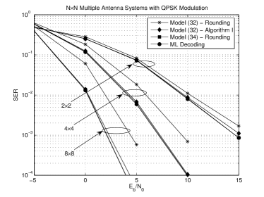
Figure 1: Performance of the proposed model (III-B) and (III-B) in a MIMO system with $N$ transmit and $N$ receive antennas employing QPSK

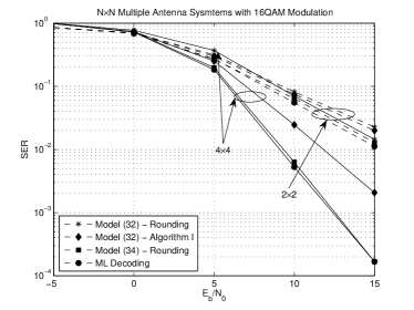
Figure 2: Performance of the proposed model (III-B) and (III-B) in a MIMO system with $N$ transmit and $N$ receive antennas employing 16-QAM

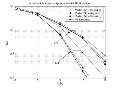
Figure 3: Performance of the proposed model (III-B) and (III-B) in a MIMO system with $N$ transmit and $N$ receive antennas employing 8-PSK

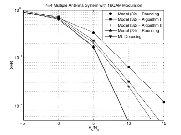
Figure 4: Different randomization algorithms in a MIMO system with $4$ transmit and $4$ receive antennas employing 16-QAM

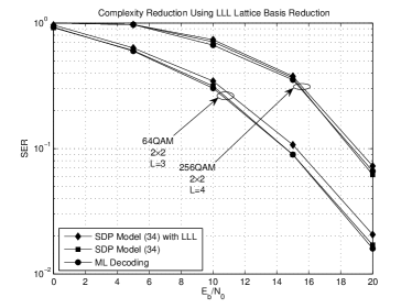
Figure 5: Performance of using LLL lattice basis reduction for relaxation model (III-B) in a $2\times 2$ MIMO system with $L=\log 2(K)$

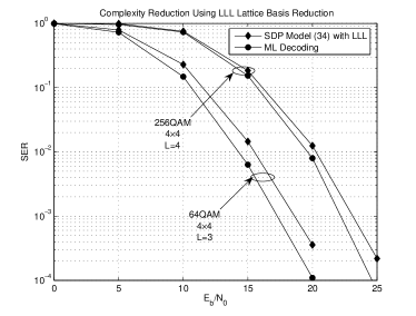
Figure 6: Performance of using LLL lattice basis reduction for relaxation model (III-B) in a $4\times 4$ MIMO system with $L=\log 2(K)$

VII-B Complexity Analysis

Semi-definite programs of reasonable size can be solved in polynomial time within any specified accuracy by IPMs. IPMs are iterative algorithms which use a Newton-like method to generate search directions to find an approximate solution to the nonlinear system. The IPMs converge vary fast and an approximately optimal solution is obtained within a polynomial number of iterations. For a survey on IPMs see [47, 48]. In the sequel, we provide an analysis for the worst case complexity of solving models (III-B) and (III-B) by IPMs.

It is known (see e.g. [49]) that a SDP with rational data can be solved, within a tolerance $\epsilon$, in $O(\sqrt{m}\log(1/\epsilon))$ iterations, where $m$ is the dimension of the matrix variable. Note that for the SDP problems (III-B) and (III-B), $m=N(K-1)+1$.

The computational complexity for one interior-point iteration depends on several factors. The main computational task in each iteration is solving a linear system an order determined by the number of constraints, $p$. This task requires $O(p^{3})$ operations. The remaining computational tasks involved in one interior-point iteration include forming system matrix whose total construction requires $O(pm^{3}+p^{2}m^{2})$ arithmetic operations. Thus, the complexity per iteration of the IPM for solving SDP problem whose matrix variable is of dimension $m$ and number of equality constraints $p$, is $O(pm^{3}+p^{2}m^{2}+p^{3})$. This means for a given accuracy $\epsilon$, an interior-point method in total requires at most $O(p(m^{3}+pm^{2}+p^{2})\sqrt{m}$ $\log(1/\epsilon))$ arithmetic operations.

Since the SDP relaxation (III-B) contains $O(K^{2}N)$ equality constraints, it follows that a solution to (III-B) can be found in at most $O(N^{4.5}K^{6.5}\log(1/\epsilon))$ arithmetic operations. SDP relaxation (III-B) contains $O(K^{2}N)$ equations and $O(K^{2}N^{2})$ sign constraints. In order to solve relaxation (III-B), we formulate the SDP model as a standard linear cone program (see e.g. [50]) by adding some slack variables. The additional inequality constraints make the model in (III-B) considerably stronger than the model in (III-B) (see numerical results), but also more difficult to solve. An interior-point method for solving SDP model (III-B) within a tolerance $\epsilon$ requires at most $O(N^{6.5}K^{6.5}\log(1/\epsilon))$ arithmetic operations. Since the problem sizes of interest are moderate, the problem in (III-B) is tractable. However, there exist a trade-off between the strength of the bounds and the computational complexity for solving these two models (see Section III).

The complexity of the randomization procedure applied to the model (III-B) is negligible compared to that of solving the problem itself. Namely, if we denote the number of randomization iterations by $N_{rand}$, then the worst case complexity of the randomization procedure is $O(NKN_{rand})$.

The problems (III-B) and (III-B) are polynomially solvable. These problems have many variables; however, they contain sparse low-rank (rank-one) constraint matrices. Exploiting the structure and sparsity characteristic of semi-definite programs is crucial to reduce the complexity. In [51], it is shown that rank-one constraint matrices (similar to our problems) reduce the complexity of the interior-point algorithm for positive semi-definite programming by a factor of $NK$. In other words, the complexities of the SDP relaxation problems (III-B) and (III-B) are decreased to $O(N^{3.5}K^{5.5}\log(1/\epsilon))$ and $O(N^{5.5}K^{5.5}\log(1/\epsilon))$, respectively. Also, implementing the rank-one constraint matrices results in a faster convergence and a saving in the computation time and memory requirements. It is worth mentioning that when we use the LLL lattice basis reduction, the value of $K$ is replaced with $L$ in the aforementioned analysis. As mentioned before, this value is much smaller than $K$, e.g. in our simulation results $L=\log_{2}(K)$, which results in reducing the computational complexity.

VII-C Comparison

The worst-case complexity of well-known SD method [24, 15] is known to be an exponential function of dimension $M$ over all ranges of rate and $S\!N\!R$ [24]. The complexity analysis shows that our proposed SDP algorithms possess a polynomial-time worst case complexity. It should be emphasized that in real time problems, the time spent for decoding the received vector is important and it can be considered as a measure of the complexity.

In the following, the worst case complexities of the algorithm based on model (III-B), the method proposed in [30], the method in [27], and the SD algorithm [15] are compared with different random values of input vector, channel matrix, and noise for $E_{b}/N_{0}=\{-5,0,5,10,15\}$. For each value of $E_{b}/N_{0}$, the algorithms are performed for $10^{5}$ times and the maximum time spent for the decoding procedure is saved in $MaxTime$. The average time spent for decoding each case is stored in $AveTime$.

It should be emphasized that the $MaxTime$ for each case depends on how the algorithm is implemented. There are numerous variants for SD algorithm. In the following, we have implemented the SD algorithm based on the Schnorr-Euchner strategy proposed in [15]. Moreover, the simulations of the proposed algorithms are implemented by one of the simplest available packages, the SDPA package [41]. However, by utilizing the sparsity of the constraint matrices as suggested in [51] and using the DSDP package, the computed $AveTime$ and $MaxTime$ can be reduced dramatically (a factor of $NK$ in the analysis), without any performance degradation.

Table I shows the simulation results for a MIMO system with $\tilde{M}=\tilde{N}=4$ employing 16-QAM. The maximum time for decoding a symbol using SD algorithm is much longer than the corresponding time in the proposed SDP relaxation method. The other three methods have comparable $MaxTime$. As it is also shown in the analysis, the proposed Model III is more complex compared to the two other SDP methods. However, this method outperforms the other SDP methods in [27] and [30].

TABLE I: Comparison of $MaxTime$ for different methods in a MIMO system with 4 transmit and 4 receive antennas employing 16-QAM

$E_{b}/N_{0}$	-5	0	5	10	15
Model III	0.1037	0.1095	0.1108	0.1178	0.1196
Method [30]	0.0685	0.0640	0.0697	0.0735	0.0624
Method [27]	0.0580	0.0633	0.0536	0.0646	0.0596
SD Method	61.8835	47.0480	28.0347	4.3848	2.2477

The relaxation model (III-B) outperforms the SDP methods proposed in [27] and [29]. Fig. 7 compares the performance of [29] and the relaxation model (III-B) and the performance of the method proposed in [27] is shown in Fig. 8 in a MIMO system with 4 transmit and receive antennas. The order of the complexity of [27] is comparable to the proposed model (III-B) and the order of the complexity of [29] is less than that of the model (III-B) ($O(N^{2})$ vs. $O(N^{3.5})$). The method in [27] can handle QAM constellations; however, it achieves near ML performance only in the case of BPSK and QPSK constellations. Also, the method in [29] is limited to PSK constellations. Note that our proposed methods can be used for any arbitrary constellation and labeling.

The comparison of the performance of the relaxation model proposed in [30] and that of our method is shown in Fig. 8 ($4\times 4$ antenna system employing $16$-QAM). It is observed that the SDP relaxation models (III-B) and (III-B) perform better than [30]. The order of the complexity of [30] is the same as that of the model (III-A), while the model (III-B) is more complex ($O(N^{5.5})$ vs. $O(N^{3.5})$).

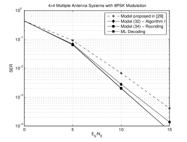
Figure 7: Comparison of the relaxation model proposed in [29] and that in our method in a MIMO system with 4 transmit and receive antennas, employing 8-PSK modulation

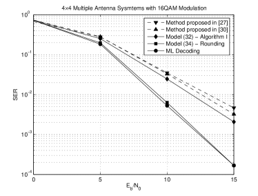
Figure 8: Comparison of the relaxation model proposed in [30] and that in our method in a MIMO system with 4 transmit and receive antennas, employing 16-QAM modulation

Although the worst case complexities of the SD algorithm [15, 24] and the other variants are exponential, in several papers, the average complexity of these algorithms are investigated. In [26], it is shown that generally, there is an exponential lower bound on the average complexity of the SD algorithm. However, it is shown that for large values of $E_{b}/N_{0}$ and small values of dimension $M$, the average complexity can be approximated by a polynomial function of dimension $M$.

In Table II, the average time $AveTime$ spent for decoding the received vectors in the previous scenario is shown. As it can be seen, the average complexity of all SDP methods is gradually increasing with $E_{b}/N_{0}$ while the average complexity of SD method is decreasing exponentially. This suggests that for different dimensions $M$ and values of $E_{b}/N_{0}$, there is a threshold that the proposed SDP methods perform better than SD algorithm even in terms of the average complexity. However, Table I shows that how inefficient SD algorithm performs in terms of the worst-case complexity.

TABLE II: Comparison of $AveTime$ for different methods in a MIMO system with 4 transmit and 4 receive antennas employing 16QAM

$E_{b}/N_{0}$	-5	0	5	10	15
Model III	0.0372	0.0377	0.0394	0.0428	0.0417
Method [30]	0.0130	0.0134	0.0142	0.0156	0.0156
Method [27]	0.0116	0.0118	0.0126	0.0141	0.0141
SD Method	0.0449	0.0139	0.0060	0.0026	0.0016

In the following, in Tables III and IV, the performance of the proposed algorithm based on Model III and SD algorithm are shown in terms of $AveTime$ and $MaxTime$, for different number of antennas and constellations. It can be seen that, in terms of the worst-case complexity the proposed algorithm based on Model III always outperforms SD algorithm. Generally, we can conclude that by increasing the dimension and rate, the range of $E_{b}/N_{0}$ that the proposed model outperforms the SD algorithm increases. In order to show that the $MaxTime$ values are not sporadic, we also provide the values of $AveMaxTime$ in Table IV. This number is the average of the largest $100$ decoding times in each case.

TABLE III: Decoding Time in a MIMO system with 4 transmit and 4 receive antennas employing QPSK

	$E_{b}/N_{0}$	-5	0	5	10	15
$AveTime$	Model III	0.0154	0.0156	0.0238	0.0278	0.0236
	SD Method	0.0199	0.0074	0.0046	0.0028	0.0020
$MaxTime$	Model III	0.4271	0.4251	0.4765	0.7572	0.8417
	SD Method	28.326	26.3109	25.4260	2.2232	0.9663

TABLE IV: Decoding Time in a MIMO system with 8 transmit and 8 receive antennas

		$E_{b}/N_{0}$	-5	0	5	10	15
QPSK	$AveTime$	Model III	0.0152	0.0152	0.0174	0.0224	0.0306
		SD Method	0.6005	0.1061	0.0319	0.0149	0.0052
	$MaxTime$	Model III	0.0965	0.0655	0.1666	0.6586	0.6959
		SD Method	433.3972	179.0310	19.7889	16.7787	7.7819
	$AveMaxTime$	Model III	0.0658	0.0587	0.0642	0.1492	0.2109
		SD Method	73.4830	16.3274	6.1652	5.9249	1.8074
16-QAM	$AveTime$	Model III	0.0936	0.0948	0.0984	0.1050	0.1059
		SD Method	42.2894	1.6575	0.4762	0.2955	0.1080
	$MaxTime$	Model III	0.2867	0.2974	0.2772	0.2916	0.3273
		SD Method	8633.8	383.40	290.89	121.92	91.032
	$AveMaxTime$	Model III	0.1574	0.1580	0.1633	0.1682	0.1712
		SD Method	411.6743	15.3724	4.5987	2.9336	1.0162

The performance of the proposed SDP relaxation model (III-B), Model IV, is close to the ML performance. Similar to the SDP relaxation model (III-B), the algorithm based on Model IV outperforms the SD algorithm in terms of the worst case complexity (polynomial vs. exponential). Furthermore, by using the LLL lattice basis reduction before the proposed SDP model, the complexity is reduced, with an acceptable degradation in the performance (as shown in Simulation Results section).

As a final note, we must emphasis that in the complexity analysis for model (III-B), we have considered all the non-negative constraints. This suggests that the complexity of this model is not tractable. However, it is not required to consider all the non-negative constraints. In order to implement this model more efficiently, we can solve the SDP relaxation (III-B), and solve the SDP relaxation (III-B) with only the most violated constraints. These constraints correspond to those positions in matrix ${\bf Y}$ where their values are the minimum negative numbers. Implementing Model IV based on the most violated constraints reduces the complexity to almost a number of times more complex compared to the Model III.

VIII Conclusion

A method for quasi-maximum likelihood decoding based on two semi-definite relaxation models is introduced. The proposed semi-definite relaxation models provide a wealth of trade-off between the complexity and the performance. The strongest model provides a near-ML performance with polynomial-time worst-case complexity (unlike the SD that has exponential-time complexity). Moreover, the soft decoding method based on the proposed models is investigated. By using lattice basis reduction the complexity of the decoding methods based on theses models is reduced.

Appendix A Lagrangian Duality

In this appendix, we show that Lagrangian duality can be used to derive the SDP relaxation problem (III-A). We first dualize the constraints of (II), and then derive the SDP relaxation from the dual of the homogenized Lagrangian dual. Finally, we project the obtained relaxation onto the minimal face. The resulting relaxation is equivalent to the relaxation (III-A).

Consider the minimization problem in (II). According to [31], for an accurate semi-definite solution, zero-one constraints should be formulated as quadratic constraints. Therefore,

$$\min\;\; \mathbf{u}^{T}\mathbf{Q}\mathbf{u}+2\mathbf{c}^{T}\mathbf{u}$$

$$s.t.\;\; \|\mathbf{A}\mathbf{u}-\mathbf{e}_{N}\|^{2}=0$$

$$u_{i}^{2}=u_{i}\;\;\forall i=1,\cdots,n.$$ (76)

First, the constraints are added to the objective function using lagrange multipliers $\lambda$ and $\mathbf{\tilde{w}}=\left[\tilde{w}_{1},\cdots,\tilde{w}_{n}\right]^{T}$:

$$\mu_{\mathcal{O}}=\min_{\mathbf{u}}\max_{\lambda,\mathbf{\tilde{w}}} \left\{\mathbf{u}^{T}\mathbf{Q}\mathbf{u}+2\mathbf{c}^{T}\mathbf{u}\right.$$

$$+\lambda\left(\mathbf{u}^{T}\mathbf{A}^{T}\mathbf{A}\mathbf{u}-2\mathbf{e}_{N}^{T}\mathbf{A}\mathbf{u}+\mathbf{e}_{N}^{T}\mathbf{e}_{N}\right)$$

$$+\sum_{i=1}^{n}\tilde{w}_{i}\left(u_{i}^{2}-u_{i}\right)\left.\right\}.$$ (77)

Interchanging min and max yields

$$\mu_{\mathcal{O}}\geq\mu_{\mathcal{L}}=\max_{\lambda,\mathbf{\tilde{w}}}\min_{\mathbf{u}} \left\{\mathbf{u}^{T}\mathbf{Q}\mathbf{u}+2\mathbf{c}^{T}\mathbf{u}\right.$$

$$+\lambda\left(\mathbf{u}^{T}\mathbf{A}^{T}\mathbf{A}\mathbf{u}-2\mathbf{e}_{N}^{T}\mathbf{A}\mathbf{u}+\mathbf{e}_{N}^{T}\mathbf{e}_{N}\right)$$

$$+\sum_{i=1}^{n}\tilde{w}_{i}\left(u_{i}^{2}-u_{i}\right)\left.\right\}.$$ (78)

Next, we homogenize the objective function by multiplying t with a constrained scalar $u_{0}$ and then increasing the dimension of the problem by $1$. Homogenization simplifies the transition to a semi-definite programming problem. Therefore, we have

$$\mu_{\mathcal{O}}\geq\mu_{\mathcal{L}}=\max_{\lambda,\mathbf{\tilde{w}}}\min_{\mathbf{u},u_{0}^{2}=1} \left\{\mathbf{u}^{T}\left[\mathbf{Q}+\lambda\mathbf{A}^{T}\mathbf{A}+\textmd{Diag}(\mathbf{\tilde{w}})\right]\mathbf{u}\right.$$

$$-\left(2\lambda\mathbf{e}_{N}^{T}\mathbf{A}-2\mathbf{c}^{T}+\mathbf{\tilde{w}}^{T}\right)u_{0}\mathbf{u}$$

$$+\lambda\mathbf{e}_{N}^{T}\mathbf{e}_{N}\left.\right\},$$ (79)

where $\textmd{Diag}(\mathbf{\tilde{w}})$ is a diagonal matrix with $\mathbf{\tilde{w}}$ as its diagonal elements. Introducing a Lagrange multiplier $w_{0}$ for the constraint on $u_{0}$, we obtain the lower bound $\mu_{\mathcal{R}}$

$$\mu_{\mathcal{O}}\geq\mu_{\mathcal{L}}\geq\mu_{\mathcal{R}}=\max_{\lambda,\mathbf{\tilde{w}},w_{0}} \min_{u_{0},\mathbf{u}}\left\{\mathbf{u}^{T}\left[\mathbf{Q}+\lambda\mathbf{A}^{T}\mathbf{A}+\textmd{Diag}(\mathbf{\tilde{w}})\right]\mathbf{u}\right.$$

$$-\left(2\lambda\mathbf{e}_{N}^{T}\mathbf{A}-2\mathbf{c}^{T}+\mathbf{\tilde{w}}^{T}\right)u_{0}\mathbf{u}$$

$$+\lambda\mathbf{e}_{N}^{T}\mathbf{e}_{N}u_{0}^{2}+w_{0}\left(u_{0}^{2}-1\right)\left.\right\}.$$ (80)

Note that both inequalities can be strict, i.e. there can be duality gaps in each of the Lagrangian relaxations. Also, the multiplication of $\lambda\mathbf{e}_{N}^{T}\mathbf{e}_{N}$ by $u_{0}^{2}$ is a multiplication by $1$. Now, by grouping the quadratic, linear, and constant terms together and defining $\mathbf{\tilde{u}}^{T}=\left[u_{0},\mathbf{u}^{T}\right]^{T}$ and $\mathbf{w}^{T}=\left[w_{0},\mathbf{\tilde{w}}^{T}\right]^{T}$, we obtain

$$\mu_{\mathcal{R}}=\max_{\lambda,\mathbf{w}}\min_{\tilde{\mathbf{u}}}\left\{\tilde{\mathbf{u}}^{T}\left[\mathcal{L}_{\mathbf{Q}}+\textmd{Arrow}(\mathbf{w})+\lambda\mathcal{L}_{\lambda}\right]\mathbf{u}-w_{0}\right\},$$ (81)

where

$$\mathcal{L}_{\lambda}=\left[\begin{tabular}[]{cc}$\mathbf{e}_{N}^{T}\mathbf{e}_{N}$&$-\mathbf{e}_{N}^{T}\mathbf{A}$\\ $-\mathbf{A}^{T}\mathbf{e}_{N}$&$\mathbf{A}^{T}\mathbf{A}$\\ \end{tabular}\right]=\left[\begin{tabular}[]{cc}$N$&$-\mathbf{e}^{T}_{K}\otimes\mathbf{e}^{T}_{N}$\\ $-\mathbf{e}_{K}\otimes\mathbf{e}_{N}$&$\mathbf{I}_{N}\otimes(\mathbf{e}_{K}\mathbf{e}^{T}_{K})$\\ \end{tabular}\right],$$ (86)

$$\textmd{Arrow}(\mathbf{w})=\left[\begin{tabular}[]{cc}$w_{0}$&$-\frac{1}{2}\mathbf{w}^{T}_{1:n}$\\ $-\frac{1}{2}\mathbf{w}_{1:n}$&$\textmd{Diag}(\mathbf{w}_{1:n})$\\ \end{tabular}\right],$$ (89)

$$\textmd{and }\mathcal{L}_{\mathbf{Q}}=\left[\begin{tabular}[]{cc}$0$&$\mathbf{c}^{T}$\\ $\mathbf{c}$&$\mathbf{Q}$\\ \end{tabular}\right].$$ (92)

Note that we will refer to the additional row and column generated by the homogenization of the problem as the 0-th row and column. There is a hidden semi-definite constraint in (81), i.e. the inner minimization problem is bounded below only if the Hessian of the quadratic form is positive semi-definite. In this case, the quadratic form has minimum value $0$. This yields the following SDP problem:

$$\max\;\; -w_{0}$$

$$s.t.\;\; \mathcal{L}_{\mathbf{Q}}+\textmd{Arrow}(\mathbf{w})+\lambda\mathcal{L}_{\lambda}\succeq 0.$$ (93)

We now obtain our desired SDP relaxation of (A) as the Lagrangian dual of (A). By Introducing the $(n+1)\times(n+1)$ dual matrix variable $\mathbf{Y}\succeq 0$, the dual program to the SDP (A) would be

$$\min\;\; \textmd{trace }\mathcal{L}_{\mathbf{Q}}\mathbf{Y}$$

$$s.t.\;\; {\rm diag}(\mathbf{Y})=(1,\mathbf{Y}_{0,1:n})^{T}$$

$$\textmd{trace}\mathbf{Y}\mathcal{L}_{\lambda}=0$$

$$\mathbf{Y}\succeq 0,$$ (94)

where the first constraint represents the zero-one constraints in (A) by guaranteeing that the diagonal and 0-th column (row) are identical (matrix ${\bf Y}$ is indexed from 0); and the constraint ${\bf Au}={\bf e}_{N}$ is represented by the constraint $\textmd{trace}\mathbf{Y}\mathcal{L}_{\lambda}=0$. Note that if the matrix $\mathbf{Y}$ is restricted to be rank-one in (A), i.e.

$$\mathbf{Y}=\left[\begin{tabular}[]{c}$1$\\ $\mathbf{u}$\\ \end{tabular}\right]\left[1\;\mathbf{u}^{T}\right],$$

for some $\mathbf{u}\in\mathbb{R}^{n}$, then the optimal solution of (A) provides the optimal solution, $\mathbf{u}$, for (A).

Since the matrix $\mathcal{L}_{\lambda}\neq 0$ is a positive semi-definite matrix; therefore, to satisfy the constraint in (A), $\mathbf{Y}$ has to be singular. This means the feasible set of the primal problem in (A) has no interior [34] and an interior-point method may never converge. However, a simple structured matrix can be found in the relative interior of the feasible set in order to project (and regularize) the problem into a smaller dimension.

As mentioned before, the rank-one matrices are the extreme points of the feasible set of the problem in (A) and the minimal face of the feasible set that contains all these points shall be found [34].

From Theorems 2 and 3, we conclude that $\mathbf{Y}\succeq 0$ is in the minimal face if and only if $\mathbf{Y}=\mathbf{\hat{V}R\hat{V}}^{T}$, for some $\mathbf{R}\succeq 0$. By substituting $\mathbf{\hat{V}R\hat{V}}^{T}$ for $\mathbf{Y}$ in the SDP relaxation (A), we get the following projected SDP relaxation which is the same as the SDP relaxation in (III-A):

$$\mu_{R1}=\min\;\; \textmd{trace }(\mathbf{\hat{V}}^{T}\mathcal{L}_{\mathbf{Q}}\mathbf{\hat{V}})\mathbf{R}$$

s.t. $$\textmd{diag}(\mathbf{\hat{V}R\hat{V}}^{T})=(1,(\mathbf{\hat{V}R\hat{V}}^{T})_{0,1:n})^{T}$$

$$\mathbf{R}\succeq 0.$$ (95)

Note that the constraint $\textmd{trace}(\mathbf{\hat{V}}^{T}\mathcal{L}_{\lambda}\mathbf{\hat{V}})\mathbf{R}=0$ can be dropped since it is always satisfied, i.e. $\mathcal{L}_{\lambda}\mathbf{\hat{V}}=0$.

Appendix B Proofs

B-A Lemma 1

Let ${\bf X}\in{\mathcal{M}}_{K\times N}$ and ${\bf e}^{T}_{K}{\bf X}={\bf e}^{T}_{N}$. Since ${\bf V}_{K\times(K-1)}$ is a $K\times(K-1)$ matrix containing a basis of the orthogonal complement of the vector of all ones, i.e., ${\bf V}_{K\times(K-1)}^{T}{\bf e}_{K}={\bf 0}$, and

$${\bf e}^{T}_{K}{\bf F}_{K\times N}={\bf e}^{T}_{N},$$ (96)

we have

$${\bf X}={\bf F}_{K\times N}+{\bf V}_{K\times(K-1)}{\bf Z},$$ (97)

where ${\bf Z}\in{\mathcal{M}}_{(K-1)\times N}$. From

$${\bf F}_{K\times N} =\frac{1}{K}({\bf E}_{K\times N}-{\bf V}_{K\times(K-1)}{\bf E}_{(K-1)\times N})$$

$$=\left[\begin{array}[]{c}{\bf 0}_{(K-1)\times N}\\ \hline\cr{\bf e}_{N}^{T}\end{array}\right],$$ (100)

and

$${\bf V}_{K\times(K-1)}{\bf Z}=\left[\begin{array}[]{c}{\bf Z}\\ \hline\cr-{\bf e}^{T}_{K-1}{\bf Z}\end{array}\right]$$ (101)

it follows that ${\bf Z}={\bf X}(1:(K-1),1:N)$.

B-B Theorem 2

Let ${\bf Y}\in{\mathcal{F}}$ be an extreme point of ${\mathcal{F}}$, i.e.

$${\bf Y}={\bf Y}_{\bf u}=\left[\begin{array}[]{c|c}1&{\bf x}^{T}\\ \hline\cr{\bf x}&{\bf xx}^{T}\end{array}\right],$$ (102)

for some ${\bf x}={\rm vec}({\bf X})$, ${\bf X}\in{\mathcal{E}}_{K\times N}$. From Lemma 1, it follows that every matrix ${\bf X}\in{\mathcal{E}}_{K\times N}$ is of the form ${\bf X}={\bf F}_{K\times N}+{\bf V}_{K\times(K-1)}\tilde{\bf X}$ where $\tilde{\bf X}={\bf X}(1:K-1,1:N)$. From the properties of the Kronecker product (see [32]), it follows

$${\bf x}={\rm vec}({\bf X}) =\frac{1}{K}({\bf e}_{KN}-({\bf I}_{N}\otimes{\bf V}_{K\times(K-1)}){\bf e}_{(K-1)N})$$

$$+({\bf I}_{N}\otimes{\bf V}_{K\times(K-1)})\tilde{\bf x},$$ (103)

where $\tilde{\bf x}={\rm vec}(\tilde{\bf X})$. Let ${\bf p}^{T}:=\left[\begin{array}[]{cc}1&\tilde{\bf x}^{T}\end{array}\right]$ and

$${\bf W}:=\left[\frac{1}{K}({\bf e}_{KN}-({\bf I}_{N}\otimes{\bf V}_{K\times(K-1)}){\bf e}_{(K-1)\times N}),{\bf I}_{N}\otimes{\bf V}_{K\times(K-1)}\right].$$ (104)

Therefore, ${\bf x}={\bf Wp}$, and

$${\bf Y}=\left[\begin{array}[]{c|c}1&{\bf p}^{T}{\bf W}^{T}\\[4.30554pt] \hline\cr{\bf Wp}&{\bf Wpp}^{T}{\bf W}^{T}\end{array}\right]=\hat{\bf V}{\bf R}\hat{\bf V}^{T},$$ (105)

where ${\bf R}:={\bf pp}^{T}$, i.e.

$${\bf R}=\left[\begin{array}[]{c|c}1&\tilde{\bf x}^{T}\\ \hline\cr\tilde{\bf x}&\tilde{\bf x}\tilde{\bf x}^{T}\end{array}\right]\succeq{\bf 0}.$$ (106)

Since $\tilde{\bf x}$ is a binary vector, it follows that $r_{ij}\in\{0,1\},~{}\forall i,j\in\{0,\ldots,N(K-1)\}$, and ${\rm diag}(\tilde{\bf x}\tilde{\bf x}^{T})=\tilde{\bf x}$. The proof follows analogously for any convex combination of the extreme points from ${\mathcal{F}}$.

B-C Theorem 3

Fix $\mathbf{u}\in\mathcal{U}$ and let

$\mathbf{Y}={\bf Y}_{\bf u}=\left[\begin{tabular}[]{c}$1$\\ $\mathbf{u}$\end{tabular}\right]\left[1\;\mathbf{u}^{T}\right].$

Considering the constraint on this vector in (34), we divide ${\bf u}$ into $N$ sub-vectors of length $K$. In each sub-vector all the elements are zero except one of the elements which is one. Therefore, there are $K^{N}$ different binary vectors in the set $\mathcal{U}$. Consider the entries of the 0-th row of $\mathbf{Y}$. Note that $y_{0,j}=1$ means that the $j$-th element of $\mathbf{u}$ is 1. In addition, there is only one element equal to $1$ in each sub-vector. Therefore, there are $K^{N-1}$ such vectors, and the components of the 0-th row of $\hat{\mathbf{Y}}$ are given by

$\hat{y}_{0,j}=\dfrac{1}{K^{N}}K^{N-1}=\dfrac{1}{K}.$

Now consider the entries of $\mathbf{Y}$ in the other rows, $Y_{i,j}$.

1. If $i=j$, then, $y_{i,j}=1$ means that the $i$-th element of the vector $\mathbf{u}$ is 1 and there are $K^{N-1}$ such vectors; therefore, the diagonal elements are

   $\hat{y}_{i,i}=\dfrac{1}{K^{N}}K^{N-1}=\dfrac{1}{K}.$

2. If $i=K(p-1)+q,\;j=K(p-1)+r,q\neq r,q,r\in\{1,\cdots,K\},p\in\{1,\cdots,N\}$, i.e. the element is an off-diagonal element in a diagonal block, then, $y_{i,j}=1$ means that the $i$-th and the $j$-th elements of $\mathbf{u}$ in a sub-vector should be 1 and this is not possible. Therefore, this element is always zero.

3. Otherwise, we consider the elements of the off-diagonal blocks of $\mathbf{Y}$. Then, $y_{i,j}=1$ means that the $i$-th and the $j$-th elements of $\mathbf{u}$ in two different sub-vectors are 1 and there are $K^{N-2}$ such vectors; therefore, the elements of the off-diagonal blocks are

   $\hat{y}_{i,i}=\dfrac{1}{K^{N}}K^{N-2}=\dfrac{1}{K^{2}}.$

This proves the representation of $\mathbf{\hat{Y}}$ in (i) in Theorem 3.

It can be easily shown that

$$\left[\begin{tabular}[]{c|c}$1$&${\bf 0}_{n}^{T}$\\ \hline\cr$-\frac{1}{K}\mathbf{e}_{n}$&$\mathbf{I}_{n}$\end{tabular}\right]\mathbf{\hat{Y}}\left[\begin{tabular}[]{c|c}$1$&$-\frac{1}{K}\mathbf{e}^{T}_{n}$\\ \hline\cr${\bf 0}_{n}$&$\mathbf{I}_{n}$\end{tabular}\right]=\left[\begin{tabular}[]{c|c}$1$&${\bf 0}_{n}^{T}$\\ \hline\cr${\bf 0}_{n}$&$\hat{\mathbf{W}}$\end{tabular}\right],$$ (107)

where $\hat{\mathbf{W}}=\dfrac{1}{K^{2}}\mathbf{I}_{N}\otimes\left(K\mathbf{I}_{K}-\mathbf{E}_{K}\right)$. Note that $\textmd{rank}(\mathbf{\hat{Y}})=1+\textmd{rank}(\mathbf{\hat{W}})$.
The eigenvalues of $\mathbf{I}_{N}$ are 1, with multiplicity $N$ and the eigenvalues of $K\mathbf{I}_{K}-\mathbf{E}_{K}$ are $K$, with multiplicity $K-1$, and 0. Note that the eigenvalues of a Kronecker product are given by the Kronecker product of the eigenvalues [32]. Therefore, the eigenvalues of $\hat{\mathbf{W}}$ are $\frac{1}{K}$, with multiplicity $N(K-1)$, and 0, with multiplicity $N$. Therefore, we have

$$\textmd{rank}(\mathbf{\hat{Y}})=1+\textmd{rank}(\mathbf{\hat{W}})=N(K-1)+1.$$ (108)

This proves (ii) in Theorem 3.

By (107) and (108), we can easily see that the eigenvalues of $\mathbf{\hat{Y}}$ are $\dfrac{1}{K}$, with multiplicity $N(K-1)$, $\dfrac{K+N}{K}$, and 0, with multiplicity $N$. This proves (iii) in Theorem 3.

The only constraint that defines the minimal face is ${\bf Au}={\bf b}$. By multiplying of both sides by ${\bf u}^{T}$ and using the fact that ${\bf u}$ is a binary vector, we obtain

$${\bf Tuu}^{T}={\bf e}_{N}\left({\rm diag}({\bf uu}^{T})\right)^{T}.$$ (109)

This condition is equivalent to

$${\bf T}\hat{\bf Y}={\bf 0}.$$ (110)

Note that ${\rm rank}({\bf T})=N$. Therefore, we have

$$\mathcal{N}(\hat{\bf Y})=\{{\bf u}:{\bf u}\in\mathcal{R}({\bf T}^{T})\}.$$

This proves (iv) in Theorem 3.

Since $\textmd{rank}(\mathbf{\hat{V}})=N(K-1)+1$ and using Theorem 2, the columns of $\mathbf{\hat{V}}$ span the range space of $\mathbf{\hat{Y}}$. This proves (v) in Theorem 3.

Appendix C Randomization Algorithm

In this appendix, we present two randomization algorithms to transform ${\bf Y}$ to a binary rank-one matrix.

C-A Algorithm I

Goemans and Williamson [52] introduced an algorithm that randomly transforms an SDP relaxation solution to a rank-one solution. This approach is used in [27] for the quasi maximum likelihood decoding of a PSK signalling. This technique is based on expressing the BPSK symbols by $\{-1,1\}$ elements. After solving the relaxation problem in [27], the Cholesky factorization is applied to the $n\times n$ matrix $\bf Y$ and the Cholesky factor ${\bf V}=[{\bf v}_{1},\ldots,{\bf v}_{n}]$ is computed, i.e. ${\bf Y}={\bf VV}^{T}$. In [27], it is observed that one can approximate the solution of the distance minimization problem, $\bf u$, using $\bf V$, i.e. $u_{i}$ is approximated using ${\bf v}_{i}$. Thus, the assignment of $-1$ or $1$ to the vectors $\{{\bf v}_{1},\ldots,{\bf v}_{n}\}$ is equivalent to specifying the elements of $\bf u$.

Figure 9: Representation of the randomization algorithm in [52]

It is shown that norms of the vectors $\{{\bf v}_{1},\ldots,{\bf v}_{n}\}$ are one, and they are inside an $n$–dimensional unit sphere [27], see Fig. 9. These vectors should be classified in two different groups corresponding to $1$ and $-1$. In order to assign $-1$ or $1$ to these vectors, the randomization procedure generates a random vector uniformly distributed in the sphere. This vector defines a plane crossing the origin. Among given vectors ${\bf v}_{i}$, $i=1,\ldots n$, all the vectors at one side of the plane are assigned to $1$ and the rest are assigned to $-1$, as shown in Fig. 9. This procedure is repeated several times and the vector $\bf u$ resulting in the lowest objective function is selected as the answer.

In our proposed approach, the variables are binary numbers. In order to implement the randomization procedure of [52], we bijectively map the computed solution of the $\{0,1\}$ SDP formulation to the solution of the corresponding $\{-1,1\}$ SDP formulation. More precisely, we use the following mapping:

$${\bf M}=\left[\begin{array}[]{c|ccc}1&0&\cdots&0\\ \hline\cr-1&2&\cdots&0\\ \vdots&\vdots&\ddots&\vdots\\ -1&0&\cdots&2\end{array}\right],$$ (115)

$${\bf Y}_{\{-1,1\}}={\bf MY}_{\{0,1\}}{\bf M}^{T},$$ (116)

where ${\bf Y}_{\{0,1\}}$ is the resulting matrix from the relaxation model (III-B) or (III-B) and ${\bf Y}_{\{-1,1\}}$ is its corresponding matrix with $\{-1,1\}$ elements. Using (115), the solution for (II) can be computed using a similar randomization method as in [27]. The computational complexity of this randomization algorithm is polynomial [27].

Considering zero-one elements in our problem, we propose a new randomization procedure inspired by [52]. This algorithm can be applied to $\{0,1\}$ formulation directly. Therefore, the complexity of the whole randomization procedure is reduced, since the preprocessing step, i.e. bijective mapping in (115), is omitted.

C-B Algorithm II

After solving the relaxation model (III-B) or (III-B), the Cholesky factorization of $\bf Y$ results in a matrix $\bf V=[{\bf v}_{1},\ldots,{\bf v}_{n}]$ such that ${\bf Y}={\bf VV}^{T}$. The matrix ${\bf Y}$ is neither binary nor rank-one. Therefore, norms of the resulting vectors ${\bf v}_{i}$ are between zero and one. These vectors are depicted in Fig. 10. Intuitively, a sphere with a random radius uniformly distributed between zero and one has the same functionality as the random plane in Fig. 9.

Figure 10: Graphic representation for the proposed randomization algorithm

In order to assign $0$ or $1$ to these vectors, the randomization procedure generates a random number, uniformly distributed between 0 and 1, as the radius of the sphere. Among given vectors ${\bf v}_{i}$, $i=1,\ldots,n$, all the vectors whose norms are larger than this number are assigned to $1$ and the rest are assigned to $0$. In another variation of this algorithm, the radius of the sphere can be fixed, and norms of these vectors are multiplied by a random number. This procedure is repeated several times and the vector $\bf u$ resulting in the smallest objective function value in (II) is selected as the solution. Simulation results confirm that the proposed method results in a slightly better performance for the lattice decoding problem compared to the first algorithm. Also, the computational complexity of the randomization algorithm is decreased, due to the removal of the preprocessing step in (115). It is worth mentioning that, according to (102) and (106), the randomization procedure can be implemented for the matrix ${\bf R}$, which results in further reduction in the computational complexity.

References

- [1] A. Mobasher, M. Taherzadeh, R. Sotirov, and A. K. Khandani, “An Efficient Quasi-Maximum Likelihood Decoding for Finite Constellations,” in Conference on Information Sciences and Systems (CISS) 2005, March 16-18 2005.
- [2] ——, “A Randomization Method for Quasi-Maximum Likelihood Decoding,” in Canadian Workshop on Information Theory, Jun. 5-8 2005.
- [3] ——, “A Near Maximum Likelihood Decoding Algorithm for MIMO Systems Based on Graph Partitioning,” in IEEE International Symposium on Information Theory, Sept. 4-9 2005.
- [4] E. Telatar, “Capacity of multi-antenna gaussian channels,” European Trans. on Telecomm. ETT, vol. 10, no. 6, pp. 585–596, November 1999.
- [5] G. J. Foschini, “Layered Space-Time Architecture for Wireless Communication in a Fading Environment when using Multi-Element Antennas,” Bell Labs Technical Journal, pp. 41–59, Autumn 1996.
- [6] K. S. Schneider, “Optimum detection of code division multiplexed signals,” IEEE Trans. Aerospace Elect. Sys., vol. AES-15, pp. 181–185, January 1979.
- [7] R. Kohno, H. Imai, and M. Hatori, “Cancellation techniques of co-channel interference in asynchronous spread spectrum multiple access systems,” Trans. Elect. and Comm. in Japan, vol. 66, pp. 416–423, May 1983.
- [8] M. Honig, U. Madhow, and S. Verdu, “Blind adaptive multiuser detection,” IEEE Trans. Inform. Theory, vol. 41, no. 4, pp. 994–960, July 1995.
- [9] Z. Xie, R. T. Short, and C. K. Rushforth, “A family of suboptimum detectors for coherent multi-user communications,” IEEE J. Select. Areas Commun., vol. 8, no. 4, pp. 683–690, May 1990.
- [10] G. D. Golden, G. J. Foschini, R. A. Valenzuela, and P. W. Wolniansky, “Detection Algorithm and Initial Laboratory Results using V-BLAST Space-Time Communication Architecture,” Electronics Letters, vol. 35, no. 1, pp. 14–16, January 1999.
- [11] M. Debbah, B. Muquet, M. de Courville, M. Muck, S. Simoens, and P. Loubaton, “A MMSE successive interference cancellation scheme for a new adjustable hybrid spread OFDM system,” in IEEE VTC, Tokyo (Japan), Spring 2000, pp. 745–749.
- [12] B. Helfrich, “Algorithms to construct Minkowski reduced and Hermit reduced lattice bases,” Theoretical Computer Sci. 41, pp. 125–139, 1985.
- [13] A. Korkine and G. Zolotareff, “Sur les formes quadratiques,” Mathematische Annalen, vol. 6, pp. 366–389, 1873 (in French).
- [14] A. K. Lenstra, H. W. Lenstra, and L. Lovsz, “Factoring polynomials with rational coefficients,” Mathematische Annalen, vol. 261, pp. 515–534, 1982.
- [15] E. Agrell, T. Eriksson, A. Vardy, and K. Zeger, “Closest point search in lattices,” IEEE Transaction on Information Theory, vol. 48, no. 8, pp. 2201–2214, Aug. 2002.
- [16] L. Babai, “On Lovasz’ lattice reduction and the nearest lattice point problem,” Combinatorica 6, pp. 1–13, 1986.
- [17] A. H. Banihashemi and A. K. Khandani, “Lattice decoding using the Korkin-Zolotarev reduced basis,” Elec. & Comp. Eng. Dept., Univ. of Waterloo, Waterloo, Ont., Canada, Tech. Rep. UW-E&CE 95-12, 1995.
- [18] ——, “On the Complexity of Decoding Lattices Using the Korkin-Zolotarev Reduced Basis,” IEEE Transactions in Information Theory, vol. IT-44, no. 1, pp. 162–171, January 1998.
- [19] W. H. Mow, “Universal Lattice Decoding: Principle and Recent Advances,” Wireless Communications and Mobile Computing, Special Issue on Coding and Its Applications in Wireless CDMA Systems, vol. 3, no. 5, pp. 553–569, Aug. 2003.
- [20] C. Windpassinger and R. F. H. Fischer, “Low-complexity near-maximum-likelihood detection and precoding for MIMO systems using lattice reduction,” in ITW2003, Paris, France, March 31-April 4 2003.
- [21] M. E. C. P. Schnorr, “Lattice basis reduction: Improved practical algorithms and solving subset sum problems,” Mathematical Programming, no. 66, pp. 181–191, 1994.
- [22] U. Fincke and M. Pohst, “Improved methods for calculating vectors of short length in a lattice, including a complexity analysis,” Mathematics of Computation, vol. 44, pp. 463–471, Apr. 1985.
- [23] M. O. Damen, A. Chkeif, and J.-C. Belfiore, “Lattice Code Decoder for Space-Time Codes,” IEEE Communications Letters, vol. 4, no. 5, pp. 161–163, May 2000.
- [24] B. Hassibi and H. Vikalo, “On Sphere Decoding Algorithm. Part I. Expected Complexity,” 2003, submitted to IEEE Transaction on Signal Processing.
- [25] G. Rekaya and J.-C. Belfiore, “Complexity of ML lattice decoders for the decoding of linear full rate Space-Time Codes,” Dec. 2002, accepted for publication in IEEE Trans. on Wireless Communications.
- [26] J. Jaldén and B. Ottersten, “On the complexity of sphere decoding in digital communications,” IEEE Trans. on Signal Proc., vol. 53, no. 4, pp. 1474–1484, 2005.
- [27] B. Steingrimsson, T. Luo, and K. M. Wong, “Soft quasi-maximum-likelihood detection for multiple-antenna wireless channels,” IEEE Transactions on Signal Processing, vol. 51, no. 11, pp. 2710– 2719, Nov. 2003.
- [28] E. Agrell, J. Lassing, E. G. Strm, and T. Ottosson, “On the optimality of the binary reflected gray code,” IEEE Trans. on Inform. Theory, vol. 50, no. 12, pp. 3170–3182, Dec 2004.
- [29] Z. Q. Luo, X. Luo, and M. Kisialiou, “An Efficient Quasi-Maximum Likelihood Decoder for PSK Signals,” in ICASSP ’03, 2003.
- [30] A. Wiesel, Y. C. Eldar, and S. Shamai, “Semidefinite relaxation for detection of 16-QAM signaling in mimo channels,” IEEE Signal Processing Letters, vol. 12, no. 9, Sept. 2005.
- [31] H. Wolkowicz, R. Saigal, and L. Vandenberghe, Handbook of Semidefinite Programming: Theory, Algorithms, and Applications. Kluwer, 2000.
- [32] A. Graham, Kronecker Products and Matrix Calculus with Applications, Mathematics and its Applications. Ellis Horwood Limited, Chichester, 1981.
- [33] H. Wolkowicz and Q. Zhao, “Semidefinite programming relaxations for the graph partitioning problem,” Discrete Applied Mathematics 96-97, pp. 461–479, 1999.
- [34] Q. Zhao, S. Karisch, F. Rendl, and H. Wolkowicz, “Semidefinite programming relaxation for the quadratic assignment problem,” J. Combinatorial Optimization, vol. 2, pp. 71–109, 1998.
- [35] R. Sotirov and F. Rendl, “Bounds for the Quadratic Assignment Problem Using the Bundle Method,” Department of Mathematics, University of Klagenfurt, Austria, Tech. Rep., 2003, available at http://www.ms.unimelb.edu.au/rsotirov.
- [36] E. Balas, S. Ceria, and G. Cornuejols, “A lift-and-project cutting plane algorithm for mixed 0–1 programs,” Mathematical Programming, vol. 58, pp. 295–324, 1993.
- [37] G. Pataki, “Algorithms for cone-optimization problems and semi-definite programming,” Graduate School of Industrial Administration, Carnegie Mellon University, Tech. Rep., 1994.
- [38] F. Alizadeh, J.-P. A. Haeberly, and M. Overton, “Primal-dual interior-point methods for semidefinite programming: Stability, convergence, and numerical results,” SIAM Journal on Optimization, vol. 8, no. 3, pp. 746–768, 1998.
- [39] S. J. Benson and Y. Ye, “DSDP5 User Guide The Dual-Scaling Algorithm for Semidefinite Programming,” Mathematics and Computer Science Division, Argonne National Laboratory, Argonne, IL, Tech. Rep. ANL/MCS-TM-255, 2004, available via the WWW site at http://www.mcs.anl.gov/benson.
- [40] J. Sturm, “Using sedumi 1.02, a matlab toolbox for optimization over symmetric cones,” Optimization Methods and Software, vol. 11-12, pp. 625–653, 1999.
- [41] M. Kojima, K. Fujisawa, K. Nakata, and M. Yamashita, “SDPA(SemiDefinite Programming Algorithm) User s Mannual Version 6.00,” Dept. of Mathematical and Computing Sciences, Tokyo Institute of Technology, 2-12-1 Oh-Okayama, Meguro-ku, Tokyo, 152-0033, Japan, Tech. Rep., 2002, available via the WWW site at http://sdpa.is.titech.ac.jp/SDPA/.
- [42] H. Yao and G. W. Wornell, “Lattice-reduction-aided detectors for MIMO communication systems,” in Global Telecommunications Conference, 2002. GLOBECOM ’02. IEEE, vol. 1, 17-21 Nov 2002, pp. 424–428.
- [43] M. O. Damen, H. E. Gamal, and G. Caire, “MMSE-GDFE Lattice Decoding for Under-determined Linear Channels,” in Conference on Information Sciences and Systems (CISS04), March 2004.
- [44] B. M. Hochwald and S. ten Brink, “Achieving near-capacity on a multiple-antenna channel,” IEEE Transactions on Communications, vol. 51, no. 3, pp. 389 –399, March 2003.
- [45] B. Steingrimsson, Z. Q. Luo, and K. M. Wong;, “Quasi-ML detectors with soft output and low complexity for PSK modulated MIMO channels,” in 4th IEEE Workshop on Signal Processing Advances in Wireless Communications (SPAWC 2003), 15-18 June 2003, pp. 427 – 431.
- [46] R. Wang and G. B. Giannakis, “Approaching MIMO Capacity with Reduced-Complexity Soft Sphere-Decoding,” in Wireless Comm. and Networking Conf, Atlanta, GA, March 21-25, 2004.
- [47] E. de Klerk, Aspects of Semidefinite Programming: Interior Point Algorithms and Selected Applications, ser. Applied Optimization. Kluwer Academic Publishers, March 2002, vol. 65.
- [48] Y. Ye, Interior Point Algorithms: Theory and Analysis, ser. Wiley Interscience series in discrete Mathematics and Optimization. John Wiley Sons, 1997.
- [49] M. Todd, “Semidefinite Optimization,” Acta Numerica, vol. 10, pp. 515–560, 2001.
- [50] J. Sturm, “Implementation of interior point methods for mixed semidefinite and second order cone optimization problems,” Optimization Methods and Software, vol. 17, no. 6, pp. 1105–1154, 2002.
- [51] S. Benson, Y. Ye, and X. Zhang, “Mixed linear and semidefinite programming for combinatorial and quadratic optimization,” Optimization Methods and Software, vol. 11-12, pp. 515–544, 1999.
- [52] M. Goemans and D. Williamson, “Improved approximation algorithms for maximum cut and satisfability problem using semidefinite programming,” Journal of ACM, vol. 42, pp. 1115–1145, 1995.