Generalized ABBA Space-Time Block Codes

Abstract

Linear space-time block codes (STBCs) of unitary rate and full diversity, systematically constructed over arbitrary constellations for any number of transmit antennas are introduced. The codes are obtained by generalizing the existing ABBA STBCs, a.k.a quasi-orthogonal STBCs (QO-STBCs). Furthermore, a fully orthogonal (symbol-by-symbol) decoder for the new generalized ABBA (GABBA) codes is provided. This remarkably low-complexity decoder relies on partition orthogonality properties of the code structure to decompose the received signal vector into lower-dimension tuples, each dependent only on certain subsets of the transmitted symbols. Orthogonal decodability results from the nested application of this technique, with no matrix inversion or iterative signal processing required. The exact bit-error-rate probability of GABBA codes over generalized fading channels with maximum likelihood (ML) decoding is evaluated analytically and compared against simulation results obtained with the proposed orthogonal decoder. The comparison reveals that the proposed GABBA solution, despite its very low complexity, achieves nearly the same performance of the bound corresponding to the ML-decoded system, especially in systems with large numbers of antennas.

I Introduction

The design of space-time codes (STCs) as building blocks of multiple-input-multiple-output (MIMO) systems [1] has been a popular research topic in wireless communications since the discovery of the Alamouti scheme [2] and the orthogonal space-time block-codes (OSTBC) [3, 4].

Although STC techniques were originally envisioned for rather modest spatial-temporal dimensions, the last few years has seen a growing interest on techniques suitable for large/scalable MIMO systems [5, 6]. Arguably, this recent owes mainly to two related developments. The first is the advance the antenna technology enabling the design of compact multi-mode antennas [7, 8, 9] which, though small in size, can provide a large number of independent channels by exploiting spatial, pattern and polarization diversities [10]. The second is the increasing popularity of distributed and cooperative systems [11, 12, 13].

These recent developments provide a rationale for the feasibility of MIMO systems of not only large but, in fact, variable dimensions. For example, in the case of compact multi-mode antennas, MIMO setups of different dimensions may occur because the number of channels effectively made available by the spatial, pattern and polarization diversities dependents on the physical scattering properties of the environment. Analogously, in the case of distributed architectures, variable MIMO setups arise naturally since the cooperative transmission can only be employed after the group of cooperating devices is assembled [14].

MIMO techniques can significantly improve both user and rate capacities (efficiencies) of wireless communications systems [15, 16]. Although space-time transmission diversity techniques in point-to-point links are known to be sub-optimum from a Shannon capacity viewpoint [17], these techniques have their extremely low-complexity to their advantage. This trade-off argument is especially compelling when considered that the capacity achieved by MIMO systems is in practice significantly limited by the use of digital modulation [18]. It is in distributed, cooperative diversity systems, however, that the flexibility of scalable space-time coding techniques have the most of their potential [19, 20].

Given the above, it is fair to say that, when considering space-time block codes as building blocks for scalable MIMO systems, modulation-independence, generalized and systematic constructibility, orthogonal (symbol-by-symbol) decodability and rate-unitariness are the most essential features to be sought. These requirements make a strong case for linear STBCs and since existing techniques such as the Alamouti scheme, the OSTBCs and the maximum-rate minimum-delay (MRMD) STBCs are either limited to a small number of antennas, or to particular constellations, or undermined by sub-unitary rateness [21, 22], many have taken upon the challenge of designing alternative solutions. To cite a few examples, the universal STCs by Gamal et al. [23], the full-rate full-diversity (FRFD) STCs by Xiaoli et al. [24], the full-rate full-diversity orthogonal STBC scheme by He et al. [25] and the variable-rate STBCs by Kim et al. [26].

Each of the above-mentioned methods are clever techniques representing a step forward in the quest for high-performing, low-complexity STBCs with no or little rate-loss. To the best of our knowledge, however, these and other similar contributions fail to simultaneously deliver a systematic design, scalable to any number of transmit antennas, applicable to arbitrary constellations and allowing a linear, symbol-by-symbol decoding method with performance comparable to that of the maximum likelihood (ML) decoder.

In this paper, a family of space-time block codes that satisfies all these objectives is introduced. The codes are obtained by generalizing the ABBA (a.k.a quasi-orthogonal) STBCs (QO-STBCs) presented in [27, 28, 29]. A linear, orthogonal decoder for the proposed generalized ABBA (GABBA) STBCs is also provided. The performance of the new codes is also studied both analytically and through computer simulations. In particular, the exact bit error rate (BER) probability of GABBA codes over uncorrelated memoryless fading channels with unequal powers and arbitrary statistics is derived under the assumption of perfect channel knowledge at the receiver and ML decoding. Comparing those results against computer simulations, it is shown that orthogonally decoded GABBA STBCs achieve nearly the same performance of achievable with the ML decoder (which is prohibitively complex for large codes and higher-order constellations), especially in systems with a relatively large number of antennas at the receiver. The transmission rates theoretically achieved by the GABBA codes are compared against the corresponding Shannon SIMO bound [16, 30], showing that GABBA codes have the potential to reach the capacity of the SIMO channel, despite the remarkably low-complexity involved in the technique.

II Systematic Construction of GABBA-STBCs

II-A Preliminaries

To the best of our knowledge, a simple and systematic method to construct linear, full(unitary)-rate, modulation-independent STBCs for any number of antennas is yet to be demonstrated. In [27], Tirkkonen et al. conjectured that larger ABBA STBCs codes could “probably be constructed by repeatedly iterating the ABBA scheme.” It will be shown here that this conjecture was almost correct, except that the generalized construction involves two distinct ABBA schemes.

Consider a vector $\mathbf{s}_{\!K}$ of symbols taken from a non-ambiguous arbitrary complex constellation $\mathcal{S}\in\mathbb{C}_{-\{0\}}^{Q}$:

$$\mathbf{s}_{\!K}\triangleq[s_{1},\cdots,s_{K}]^{\textup{T}}\in\mathcal{S}^{K\times 1},$$ (1)

where ${}^{\textup{T}}$ denotes transpose.

Definition 1 (Linear Space-time Block Encoding Matrix)

The term linear space-time block encoding matrix will be used throughout this paper in reference to matrices of the form

$$\mathbf{C}(\mathbf{s}_{\!K}\!)=\left[\begin{array}[]{ccc}c_{1,1}&\cdots&c_{1,K}\\[-4.09024pt] \vdots&\ddots&\vdots\\[-3.22916pt] c_{K,1}&\cdots&c_{K,K}\end{array}\right]\in\mathbb{C}_{-\{0\}}^{K\times n_{t}},$$ (2)

where each element $c_{i,j}$ relates to one and only one symbol $s_{k}\in\mathbf{s}_{\!K}$, such that $c_{i,j}\in\{s_{k},-s_{k},s_{k}^{*},-s_{k}^{*}\}$. ∎

Notice that definition 1 rules out constructions based on linear combinations of entries of the symbol vector, such as the rate $3/4$ code that appears in [3].

Definition 2 (Raw Symbol, Raw Encoding Matrix)

The symbol $s_{k}$ from which an entry $c_{i,j}$ of a linear space-time block encoding matrix $\mathbf{C}(\mathbf{s}_{\!K}\!)$ derives, is referred to as the raw symbol of $c_{i,j}$, and is denoted by $\langle c_{i,j}\rangle$. Likewise, the matrix $\langle\mathbf{C}(\mathbf{s}_{\!K})\rangle$ consisting of the raw symbols of the space-time block encoding matrix $\mathbf{C}(\mathbf{s}_{\!K})$ is referred to as the raw encoding matrix of $\mathbf{C}(\mathbf{s}_{\!K})$. ∎

Definition 3 (Dense STBCs)

A linear space-time block code matrix $\mathbf{C}(\mathbf{s}_{\!K}\!)$ is said to be dense if and only if (iff) $\langle c_{i,j}\rangle\neq 0\ \forall\ (i,j)$. ∎

Definition 4 (Complete STBCs)

A linear space-time block code matrix $\mathbf{C}(\mathbf{s}_{\!K}\!)$ is said to be complete iff it satisfies both the following conditions:

• $\begin{array}[]{lcl}\langle\mathbf{c}_{i,\downarrow}\!(\mathbf{s}_{\!K})\rangle\neq\langle\mathbf{c}_{j,\downarrow}\!(\mathbf{s}_{\!K})\rangle&\forall&i\neq j\end{array}$,

• $\begin{array}[]{lcl}\langle\mathbf{c}_{\downarrow,i}\!(\mathbf{s}_{\!K})\rangle\neq\langle\mathbf{c}_{\downarrow,j}\!(\mathbf{s}_{\!K})\rangle&\forall&i\neq j\end{array}$. ∎

In plain words, if the rows and columns of an encoding channel matrix represent different transmit epochs and different transmit spatial channels, respectively, definition 3 implies that at every transmit epoch, all diversity branches are utilized. On the other hand, according to definition 4, the raw columns and raw rows of a complete encoding matrix $\mathbf{C}(\mathbf{s}_{\!K}\!)$ are, simultaneously, mutually exclusive permutations of $\mathbf{s}_{\!K}$ and $\mathbf{s}_{\!K}^{\textup{T}}$, respectively. These two properties ensure that the code fully exploits the “raw diversity” of the channel, as defined in [27, section II, $\S 1$]. Notice that the $K$-by-$n_{t}$ rectangular matrices resulting from column partitions of a dense and complete linear space-time block encoding matrix $\mathbf{C}(\mathbf{s}_{\!K}\!)$ preserve this property. For simplicity, such matrices will also be, therefore, referred to as dense and complete.

Definition 5 (Rate)

The rate of a linear space-time block code described by the matrix $\mathbf{C}(\mathbf{s}_{\!K}\!)$ is defined as the ratio between the number of independent raw symbols and the number of linearly independent rows in $\mathbf{C}(\mathbf{s}_{\!K}\!)$. ∎

Notice that, according to definition 5, a linear space-time block code as defined here can, at most, achieve a unitary rate. Therefore, the terms rate-one and full-rate will be hereafter used interchangeably in reference to a linear STBCs of rate $1$.

Definition 6 (Real Orthogonality)

A pair of vectors $\mathbf{a}$ and $\mathbf{b}$ $\in\mathbb{C}^{n\times 1}$ is said to be real orthogonal to one another iff

$$\mathbf{a}^{\textup{T}}\!\cdot\!\mathbf{b}\equiv\mathbf{b}^{\textup{T}}\!\cdot\!\mathbf{a}=\sum\limits_{i=1}^{n}a_{i}b_{i}=0.\vspace{-1em}$$ (3)

∎

Definition 6 is introduced in order make clear the distinction between the orthogonality property given in equation (3) and the notion of vector orthogonality which is usually defined, in complex Hilbert spaces, over the product of a vector against the transpose-conjugate of another [31].

Definition 7 (Block-orthogonal STBCs)

A matrix $\mathbf{C}\in\mathbb{C}^{n\times m}$ is said to be block-orthogonal iff there exists a permutation $\boldsymbol{\mathcal{C}}$ of $\mathbf{C}$ such that

$$\boldsymbol{\mathcal{C}}\cdot\boldsymbol{\mathcal{C}}^{\textup{H}}=\left[\begin{array}[]{cc}\mathbf{D}_{1}&\mathbf{0}\\ \mathbf{0}&\mathbf{D}_{2}\end{array}\right]\!,$$ (4)

where ${}^{\textup{H}}$ denotes Hermitian.

Furthermore, $\mathbf{C}$ is said to be real block-orthogonal iff a permutation $\boldsymbol{\mathcal{C}}$ exists such that

$$\boldsymbol{\mathcal{C}}\cdot\boldsymbol{\mathcal{C}}^{\textup{T}}=\left[\begin{array}[]{cc}\mathbf{D}_{1}&\mathbf{0}\\ \mathbf{0}&\mathbf{D}_{2}\end{array}\right]\!.\vspace{-1.5em}$$ (5)

∎

Definitions $6$ and $7$ establish a slight generalization of the concept of quasi-orthogonality, in the sense presented in [27, 28, 29], with quasi-orthogonality resulting in the special case where the dimensions of $\mathbf{D}_{1}$ and $\mathbf{D}_{2}$ are identical. The notion of real orthogonality will be used later in the derivation of the GABBA orthogonal decoder, in section IV.

Definition 8 (Manifold Matrices)

Consider the generating function defined below over the space of complex-valued square matrices $\mathbf{A},\mathbf{B}\in\mathbb{C}^{K\times K}$,

$$X(\mathbf{A},\mathbf{B})\triangleq\left[\!\!\!\begin{array}[]{rc}\mathbf{A}&\!\!\!\mathbf{B}\\ -\mathbf{B}&\!\!\!\mathbf{A}\\ \end{array}\!\!\right]\!\!.$$ (6)

The $1^{\textup{st}}$ order ABBA manifold matrix of the vector $\mathbf{s}_{2}=[s_{1},s_{2}]$, denoted by $\mathbf{X}_{[s_{1},s_{2}]}$, is defined as the outcome of $X(s_{1},s_{2})$, with $s_{i}\in\mathcal{S}$. Accordingly, the $2^{\textup{nd}}$ order ABBA manifold matrix of the symbol vector $\mathbf{s}_{4}\!=\![s_{1},s_{2},s_{3},s_{4}]$ with generating function $X$ is defined as the outcome of $X(\mathbf{X}_{[s_{1},s_{2}]},\mathbf{X}_{[s_{3},s_{4}]})$ and denoted by $\mathbf{X}^{2}_{[s_{1},s_{2},s_{3},s_{4}]}$.

In general, the $n$-th order ABBA manifold matrix of the vector $\mathbf{s}_{\!K}$ with generating function $X$ is defined as the outcome of $X(\mathbf{X}^{(n-1)}_{\mathbf{s}_{\!K\!/2}},\mathbf{X}^{(n-1)}_{\tilde{\mathbf{s}}_{\!K\!/2}})$ and denoted by $\mathbf{X}^{n}_{\mathbf{s}_{\!K}}$, where $\tilde{\mathbf{s}}_{\!K\!/2}$ is the complementary symbol given below

$$\tilde{\mathbf{s}}_{\!K\!/2}\triangleq[s_{\!K\!/2+1},\cdots,s_{\!K}]^{\textup{T}}.\vspace{-1em}$$ (7)

∎

Lemma 1 (Commutativeness of n-th Order Manifold Matrices)

The $n$-th order manifold matrices of independent, equal-sized vectors $\mathbf{a}_{\!K}$ and $\mathbf{b}_{\!K}\in\mathbb{C}^{K\times 1}$ commute with respect to matrix product.

Proof:

Let us rewrite $\mathbf{X}^{n}_{\mathbf{a}_{\!K}}$ and $\mathbf{X}^{n}_{\mathbf{b}_{\!K}}$ in terms of their half block-partitions:

$$\mathbf{X}^{n}_{\mathbf{a}_{K}}\!\equiv\!\!\left[\!\!\!\begin{array}[]{cl}\ \ \ \ \!\mathbf{X}^{(n\!-\!1\!)}_{\mathbf{a}_{\!K\!/2}}&\!\!\!\!\mathbf{X}^{(n\!-\!1\!)}_{\tilde{\mathbf{a}}_{\!K\!/2}}\\ -\mathbf{X}^{(n\!-\!1\!)}_{\tilde{\mathbf{a}}_{\!K\!/2}}&\!\!\!\!\mathbf{X}^{(n\!-\!1\!)}_{\mathbf{a}_{\!K\!/2}}\end{array}\!\!\!\!\right]\!\!=\!\!\left[\!\!\!\!\begin{array}[]{rl}\ \mathbf{A}_{1}&\!\!\!\!\mathbf{B}_{1}\\ -\mathbf{B}_{1}&\!\!\!\!\mathbf{A}_{1}\end{array}\!\!\!\!\right]\!\!,\vspace{-0.5em}$$ (8)

$$\mathbf{X}^{n}_{\mathbf{b}_{K}}\!\equiv\!\!\left[\!\!\!\begin{array}[]{cl}\ \ \ \ \!\mathbf{X}^{(n\!-\!1\!)}_{\mathbf{b}_{\!K\!/2}}&\!\!\!\!\mathbf{X}^{(n\!-\!1\!)}_{\tilde{\mathbf{b}}_{\!K\!/2}}\\ -\mathbf{X}^{(n\!-\!1\!)}_{\tilde{\mathbf{b}}_{\!K\!/2}}&\!\!\!\!\mathbf{X}^{(n\!-\!1\!)}_{\mathbf{b}_{\!K\!/2}}\end{array}\!\!\!\!\right]\!\!=\!\!\left[\!\!\!\!\begin{array}[]{rl}\mathbf{A}_{2}&\!\!\!\!\mathbf{B}_{2}\\ -\mathbf{B}_{2}&\!\!\!\!\mathbf{A}_{2}\end{array}\!\!\!\right]\!\!.$$ (9)

Writing the products $\mathbf{X}^{n}_{\mathbf{a}_{K}}\!\cdot\mathbf{X}^{n}_{\mathbf{b}_{K}}$ and $\mathbf{X}^{n}_{\mathbf{b}_{K}}\!\cdot\mathbf{X}^{n}_{\mathbf{a}_{K}}$ explicitly and using standard block-partition properties we obtain,

$$\mathbf{X}^{n}_{\mathbf{a}_{\!K}}\!\cdot\mathbf{X}^{n}_{\mathbf{b}_{\!K}}\!\!=\!\left[\!\!\!\begin{array}[]{cc}\mathbf{A}_{1}\!\cdot\!\mathbf{A}_{2}\!-\!\mathbf{B}_{1}\!\cdot\!\mathbf{B}_{2}&\!\!\!\mathbf{A}_{1}\!\cdot\!\mathbf{B}_{2}\!+\!\mathbf{B}_{1}\!\cdot\!\mathbf{A}_{2}\\ -(\mathbf{A}_{1}\!\cdot\!\mathbf{B}_{2}\!+\!\mathbf{B}_{1}\!\cdot\!\mathbf{A}_{2})&\!\!\!\mathbf{A}_{1}\!\cdot\!\mathbf{A}_{2}\!-\!\mathbf{B}_{1}\!\cdot\!\mathbf{B}_{2}\end{array}\!\!\!\right]\!\!,\vspace{-0.1em}$$ (10)

$$\mathbf{X}^{n}_{\mathbf{b}_{\!K}}\!\cdot\!\mathbf{X}^{n}_{\mathbf{a}_{\!K}}\!\!=\!\left[\!\!\!\begin{array}[]{cc}\mathbf{A}_{2}\!\cdot\!\mathbf{A}_{1}\!-\!\mathbf{B}_{2}\!\cdot\!\mathbf{B}_{1}&\!\!\!\mathbf{A}_{2}\!\cdot\!\mathbf{B}_{1}\!+\!\mathbf{B}_{2}\!\cdot\!\mathbf{A}_{1}\\ -(\mathbf{A}_{2}\!\cdot\!\mathbf{B}_{1}\!+\!\mathbf{B}_{2}\!\cdot\!\mathbf{A}_{1})&\!\!\!\mathbf{A}_{2}\!\cdot\!\mathbf{A}_{1}\!-\!\mathbf{B}_{2}\!\cdot\!\mathbf{B}_{1}\end{array}\!\!\!\right]\!\!.$$ (11)

It is clear from equations (10) and (11) that the condition for the $n$-th order manifold matrices $\mathbf{X}^{n}_{\mathbf{a}_{\!K}}$ and $\mathbf{X}^{n}_{\mathbf{b}_{\!K}}$ to commute is that their minors $\mathbf{A}_{1}$, $\mathbf{B}_{1}$, $\mathbf{A}_{2}$ and $\mathbf{B}_{2}$ commute. These minors are, in turn, $(n\!-\!\!1\!)$-th order manifold matrices (see equations (8) and (9)) and, therefore, commute under the same condition. Since the minors of first-order ABBA manifold matrices are complex scalars, the commutativeness of $\mathbf{X}^{n}_{\mathbf{a}_{\!K}}$ and $\mathbf{X}^{n}_{\mathbf{b}_{\!K}}$ with respect to matrix product follows immediately, by induction. ∎

II-B GABBA Encoding Matrices

We can now introduce the major result of this section.

Theorem 1 (Construction of GABBA Matrices)

For any given number of transmit antennas $n_{t}\in\mathbb{N}^{+}$, there exists a dense, complete and block-orthogonal GABBA matrix for rate-one space-time block encoded transmission of symbols taken from any complex-valued arbitrary constellation $\mathcal{S}$.

Proof:

The proof is constructive. For any given $n_{t}$, let $n\!=\!\lceil\log_{2}n_{t}\!\rceil$ and $K=2^{n}$, where $\lceil x\rceil$ denotes the smallest integer greater or equal to $x$. Next, construct the $(n\!\!-\!\!1\!)$-th order ABBA manifold matrix $\mathbf{X}^{(n\!-\!1\!)}_{\mathbf{s}_{\!K\!/2}}$ of the symbol vector $\mathbf{s}_{\!K\!/2}$, and the $(n\!\!-\!\!1\!)$-th ABBA order manifold matrix $\mathbf{X}^{(n\!-\!1\!)}_{\tilde{\mathbf{s}}_{\!K\!/2}}$ of the complimentary symbol vector $\tilde{\mathbf{s}}_{\!K\!/2}$, both with the generating function $X$ given in equation (6).

Next, construct the dense and complete GABBA mother encoding matrix $\mathbf{C}(\mathbf{s}_{\!K}\!)$ by computing

$$\mathbf{C}(\mathbf{s}_{\!K}\!)=\mathbf{Y}^{n}_{\!\mathbf{s}_{\!K}}=Y(\mathbf{X}^{(n\!-\!1\!)}_{\mathbf{s}_{\!K\!/2}},\mathbf{X}^{(n\!-\!1\!)}_{\tilde{\mathbf{s}}_{\!K\!/2}}),$$ (12)

with $Y(\mathbf{A},\mathbf{B})$ defined as

$$Y(\mathbf{A},\mathbf{B})\triangleq\left[\!\!\!\begin{array}[]{cl}\ \mathbf{A}&\!\!\!\mathbf{B}\\ -\mathbf{B}^{\textup{H}}&\!\!\!\mathbf{A}^{\textup{H}}\\ \end{array}\!\!\right]\!\!.$$ (13)

For obvious reasons, $Y(\mathbf{A},\mathbf{B})$ is referred to as the wrapping function.

Notice that the manifold matrices $\mathbf{X}^{(n\!-\!i\!)}$ are constructed over $2^{(n\!-\!i\!)}$ vectors each carrying a mutually exclusive partition of $\mathbf{s_{K}}$ tuples of symbols and, furthermore, that at each iteration of $X$, these arguments are in opposite quadrants of the resulting matrix. The same occurs with the final “wrapping” operation, $i.e.$, the application of equation (13). It is therefore clear that the GABBA mother encoding matrices are dense and complete.

It is also evident that $\mathbf{Y}^{n}_{\!\mathbf{s}_{\!K}}$ are square matrices of size $K=2^{n}$. Therefore, the capital scalar $K$ will, hereafter, exclusively denote integer powers of two. Rectangular ($K$–by–$n_{t}$) GABBA encoding matrix are obtained by simply selecting any $n_{t}$ columns of $\mathbf{C}(\mathbf{s}_{\!K}\!)$. Since columnwise partition does not affect the density and completeness of $\mathbf{C}(\mathbf{s}_{\!K}\!)$, GABBA encoding matrices $\mathbf{C}_{\!n_{t}}$ are also dense and complete, which concludes the proof. ∎

Hereafter we shall simplify the notation slightly and write $\mathbf{C}_{\!K}$, instead of $\mathbf{C}(\mathbf{s}_{\!K}\!)$, for the $K$-by-$K$ GABBA mother encoding matrix. Accordingly, the matrix obtained by selecting $n_{t}$ columns of $\mathbf{C}_{\!K}$ will be denoted by $\mathbf{C}_{\!n_{t}}$.

The following property is an immediate consequence of Theorem 1.

Corollary 1 (Block-orthogonality of GABBA Encoding Matrices)

GABBA mother encoding matrices are quasi-orthogonal and GABBA encoding matrices are block-orthogonal.

Proof:

The $K$–by–$K$ GABBA mother encoding matrix is given by

$$\mathbf{C}(\mathbf{s}_{\!K}\!)\!\triangleq\!\!\left[\!\!\!\begin{array}[]{cc}\ \ \ \!\mathbf{X}^{(n\!-\!1\!)}_{\mathbf{s}_{\!K\!/2}}&\!\!\!\!\!\mathbf{X}^{(n\!-\!1\!)}_{\tilde{\mathbf{s}}_{\!K\!/2}}\\ -\!\left(\!\mathbf{X}^{(n\!-\!1\!)}_{\tilde{\mathbf{s}}_{\!K\!/2}}\!\right)^{\textup{\!\!H}}&\!\!\!\!\left(\mathbf{X}^{(n\!-\!1\!)}_{\mathbf{s}_{\!K\!/2}}\right)^{\textup{\!\!H}}\end{array}\!\!\!\!\right]\!\!=\!\!\left[\!\!\!\!\begin{array}[]{cl}\ \mathbf{A}&\!\!\!\!\mathbf{B}\\ -\mathbf{B}^{\textup{H}}&\!\!\!\!\mathbf{A}^{\textup{\!H}}\end{array}\!\!\!\right]\!\!.$$ (14)

Writing the product $\mathbf{C}(\mathbf{s}_{\!K}\!)\!\cdot\!\mathbf{C}(\mathbf{s}_{\!K}\!)^{\textup{H}}$ explicitly, and after trivial algebraic manipulations, we obtain

$$\mathbf{C}(\mathbf{s}_{\!K}\!)\!\cdot\!\mathbf{C}(\mathbf{s}_{\!K}\!)^{\textup{H}}\!=\!\left[\!\!\!\begin{array}[]{cc}\mathbf{A}\!\cdot\!\mathbf{A}^{\textup{\!H}}+\mathbf{B}\!\cdot\!\mathbf{B}^{\textup{\!H}}&\!\!\!\mathbf{B}\!\cdot\!\mathbf{A}-\mathbf{A}\!\cdot\!\mathbf{B}\\ (\mathbf{B}\!\cdot\!\mathbf{A}-\mathbf{A}\!\cdot\!\mathbf{B})^{\textup{\!H}}&\!\!\mathbf{A}\!\cdot\!\mathbf{A}^{\textup{\!H}}+\mathbf{B}\!\cdot\!\mathbf{B}^{\textup{\!H}}\end{array}\!\!\!\right]\!\!.$$ (15)

Equation (15) indicates that the quasi-orthogonality of GABBA mother matrices is conditioned on the commutativeness of its minors $(\mathbf{A},\mathbf{B})$ and, therefore, follows directly from Lemma $1$.

Rectangular ($K$–by–$n_{t}$) GABBA matrices $\mathbf{C}_{\!n_{t}}$ are obtained by arbitrarily selecting $n_{t}$ columns of $\mathbf{C}(\mathbf{s}_{\!K}\!)$, that is, by selection a total of $n_{t}$ column vectors out of the sets $\{\mathbf{c}_{\downarrow,1}\!(\mathbf{s}_{\!K}),\cdots,\mathbf{c}_{\downarrow,K\!/2}\!(\mathbf{s}_{\!K})\}$ and $\{\mathbf{c}_{\downarrow,{1+K\!/2}}\!(\mathbf{s}_{\!K}),\cdots,\mathbf{c}_{\downarrow,K}\!(\mathbf{s}_{\!K})\}$. Since this columnwise partition does not affect the orthogonality between these two sets, the corresponding mother encoding matrix, $\mathbf{C}_{\!n_{t}}$ are obviously block-orthogonal, which concludes the proof. ∎

An example of a GABBA mother encoding matrix with $K=32$ and a Matlab implementation of the encoder described in this section are given in Appendix A. The reader is encouraged to inspect the example provided and to utilize the program in order to generate GABBA matrices of various sizes and verify their block-orthogonality.

III Quasi-Orthogonal Decoding GABBA Codes

III-A Preliminaries

Consider the problem of decoding the received signal vector corresponding to the transmission of a GABBA matrix $\mathbf{C}_{n_{t}}$ through a memoryless block-fading channel $\mathbf{h}_{\!n_{t}}$ in the presence of an additive noise vector $\mathbf{n}_{\!K}$. At a given receive antenna, such a received signal vector can be modeled as

$$\mathbf{r}=\mathbf{C}_{n_{t}}\!\cdot\mathbf{h}_{\!n_{t}}+\mathbf{n}_{\!K}=\mathbf{H}_{\!K}\cdot\bar{\mathbf{s}}_{\!K}+\mathbf{n}_{\!K},$$ (16)

where $\bar{\mathbf{s}}_{\!K}$ is the augmented symbol vector, defined as

$$\bar{\mathbf{s}}_{\!K}\triangleq[s_{1},\cdots,s_{K},s_{1}^{*},\cdots,s_{K}^{*}]^{\textup{T}},$$ (17)

where ^∗ denotes complex conjugate.

Examples of the use of alternative representations of the linear STBC receive vector, similar to that given in equation (16), can be found in the literature. For instance, in [32], the idea was employed in order derive a simpler decoder for OSTBCs, and in [29], the transformation was used to construct the quasi-orthogonal decoder for the $4$-by-$4$ code there proposed.

We have shown, however, that this technique can be expanded well beyond the relatively straightforward applications suggested in [32] and [29]. In particular, we have shown in [33, 34] that a more elaborate utilization of these transformation can be exploited to construct a novel decoder for OSTBCs which enables its use in time-selective fading channels. In this section, we build on the concepts laid in [33, 34] in order to show that GABBA codes are indeed orthogonally decodable.

III-B Structure of GABBA Encoded Channel Matrices

Equation (16) indicates that $\mathbf{H}_{\!K}$ are constructed by simply re-arranging the corresponding channel entries appropriately. These matrices are, therefore, hereafter referred to as the GABBA encoded channel matrices.

Begin by noticing that when the transmitter has a number $n_{t}\!<\!K$ of antennas, an $n_{t}$ column-partition of the corresponding $K$-by-$K$ GABBA mother encoding matrix is utilized. Mathematically, this is equivalent to the case when $K-n_{t}$ columns of $\mathbf{C}_{\!K}$ and rows of $\mathbf{h}$ (corresponding to the “unused” antennas) assume zero values, leading to a sparse $\mathbf{H}_{\!K}$, but leaving unaffect its real quasi-orthogonality properties. It is, therefore, sufficient to consider mother matrices $\mathbf{H}_{\!K}$ when studying the properties of GABBA encoded channel matrices $\mathbf{H}_{\!n_{t}}$.

Before we proceed, let us introduce some additional terminology .

Definition 9 (Notation for Matrix Partitions)

The symbol $[\mathbf{A}]^{\textup{P}:p}$ denotes the left (P=L), right (P=R), upper (P=U) or lower (P=D) partition of the matrix $\mathbf{A}$, containing its $p$ leftmost, rightmost,uppermost and lowermost columns/rows, respectively.

Definition 10 (Notation for Matrix Reorientation)

The symbols $\mathbf{A}^{\!\dagger}$ and $\mathbf{A}^{\!\ddagger}$ denote, respectively, the bottom-up and the left-to-right reorientations of a matrix $\mathbf{A}$ (a.k.a. flip upside-down and flip left-right operations). Trivial properties of these operations are:

$$\left(\mathbf{A}^{\!\dagger}\right)^{\!\dagger}=\mathbf{A},$$ (18a)

$$\mathbf{A}^{\!\dagger}\!\cdot\!\mathbf{b}=\left(\mathbf{A}\!\cdot\!\mathbf{b}\right)^{\dagger}=\mathbf{A}^{\!\dagger\ddagger}\!\cdot\!\mathbf{b}^{\dagger}\!\!.$$ (18b)

where $$\mathbf{A}\in\mathbb{C}^{n\times m} \mathbf{b}\in\mathbb{C}^{m\times 1}$$ and .

Next, observe that due to the structures of $\mathbf{C}_{\!K}$ and $\bar{\mathbf{s}}_{\!K}$, $\mathbf{H}_{\!K}$ can be written as

$$\mathbf{H}_{\!K}=\left[\begin{array}[]{cc}\mathbf{H}_{\!K_{1}}\!\!&\!\!\mathbf{0}\!\!\\ \mathbf{0}\!\!&\!\!\mathbf{H}_{\!K_{2}}\!\!\\ \end{array}\right]\!\!,$$ (19)

where $\mathbf{H}_{\!K_{1}}$ and $\mathbf{H}_{\!K_{2}}$ are both $K\!/2$–by–$K$ matrices.

The following result can then be stated and proved.

Lemma 2 (Construction of GABBA Encoded Channel Matrices)

The non-zero minors $\mathbf{H}_{\!K_{1}}$ and $\mathbf{H}_{\!K_{2}}$ of the GABBA encoded channel matrix $\mathbf{H}_{\!K}$ are given by

$$\mathbf{H}_{\!K_{1}}=[\mathbf{H}^{n}_{\mathbf{h}_{\!K}^{+}}]^{\textup{U}:K\!/2}\!,$$ (20)

$$\mathbf{H}_{\!K_{2}}=[\tilde{\mathbf{H}}^{n}_{\mathbf{h}_{\!K}^{\circlearrowright}}]^{\textup{U}:K\!/2}\!,$$ (21)

where $\mathbf{H}^{n}_{\mathbf{h}_{\!K}^{+}}$ and $\tilde{\mathbf{H}}^{n}_{\mathbf{h}_{\!K}^{\circlearrowright}}$ are $n$-th order manifold matrices of the extended channel vector $\mathbf{h}_{\!K}^{+}$ and the modified channel vector $\mathbf{h}^{\circlearrowright}_{\!K}$, respectively,

$$\mathbf{h}_{\!K}^{+}\triangleq[\underbrace{h_{1},\cdots,0,\cdots,h_{k},\cdots,0,\cdots,h_{n_{t}},\cdots,0}_{\mathbf{h}_{n_{t}}\textup{ extended with }K-n_{t}\textup{ zero-entries}}]^{\textup{T}}\!,$$ (22)

$$\mathbf{h}^{\circlearrowright}_{\!K}\triangleq[[\mathbf{h}_{\!K}^{+}]^{\textup{D}:K\!/2}\ [\mathbf{h}_{\!K}^{+}]^{\textup{U}:K\!/2}]=[\underbrace{h_{\!K\!/2+1},\cdots,0,\cdots,h_{n_{t}},\cdots,0}_{\textup{last }K\!/2\textup{ entries of }\mathbf{h}_{\!K}^{+}}\underbrace{,h_{1},\cdots,h_{k},\cdots,0,\cdots,h_{\!K\!/2}}_{\textup{first }K\!/2\textup{ entries of }\mathbf{h}_{\!K}^{+}}]^{\textup{T}}\!,$$ (23)

with the corresponding generating functions $H$ and $\tilde{H}$ given by

$$H(\mathbf{A},\mathbf{B})\triangleq\left[\!\!\!\begin{array}[]{cr}\mathbf{A}&\!\!\!\mathbf{B}\\ \mathbf{B}&\!\!\!-\mathbf{A}\\ \end{array}\!\!\right]\!\!,$$ (26)

$$\tilde{H}(\mathbf{A},\mathbf{B})\triangleq\left[\!\!\!\begin{array}[]{cr}\mathbf{A}&\!\!\!-\mathbf{B}\\ \mathbf{B}&\!\!\!\mathbf{A}\\ \end{array}\!\!\right]\!\!.$$ (29)

Proof:

The proof is constructive. The noise-independent terms of the first $K/2$ entries of $\mathbf{r}$ can be written as

[[𝐂K]U:K2]D:2]⋅[h1h2[𝐡]D:(K−2)]=[ [𝐇K1]D:(K/2−2)]⋅[s1s2[𝐬]D:(K−2)]=𝐇K1⋅𝐬K.⋅superscriptdelimited-[]subscript𝐂subscript𝑛𝑡:U𝐾2𝐡⋅delimited-[]fragments fragments[[C𝐾]:U𝐾2]:D2delimited-[]subscriptℎ1subscriptℎ2missing-subexpressionmissing-subexpressionsuperscriptdelimited-[]𝐡:D𝐾2⋅delimited-[]fragments fragments[Hsubscript𝐾1]:D𝐾22delimited-[]subscript𝑠1subscript𝑠2missing-subexpressionmissing-subexpressionsuperscriptdelimited-[]𝐬:D𝐾2⋅subscript𝐇subscript𝐾1subscript𝐬𝐾\displaystyle[\mathbf{C}_{\!n_{t}}]^{\textup{U}:\tfrac{K}{2}}\!\cdot\mathbf{h}\!\!=\!\!\!\left[\begin{tabular}[]{cc}$\begin{array}[]{rl}\!\!\!\!\!\!s_{1}&\!\!\!s_{2}\\ \!\!\!\!\!\!-s_{2}&\!\!\!s_{1}\end{array}$ \!\!\!\!\vline\!\!\!\!&\!\!\!\! $\left[[\mathbf{C}_{\!K}]^{\textup{U}:2}\right]^{\!\textup{R}:(\!K-\!2)}$\!\!\!\!\\ \hline\cr\\[-17.22217pt] \lx@intercol\hfil$\big{[}[\mathbf{C}_{\!K}]^{\textup{U}:\tfrac{K}{2}}\big{]}^{\textup{D}:2}$\hfil\lx@intercol\!\!\!\!\\ \end{tabular}\right]\!\!\cdot\!\!\left[\begin{array}[]{c}\!\!\!h_{1}\!\!\!\!\!\\ \!\!\!h_{2}\!\!\!\!\!\\ \hline\cr\\[-17.22217pt] \!\!\![\mathbf{h}]^{\textup{D}:(\!K-\!2)}\!\!\!\!\!\\ \end{array}\right]\!\!\!=\!\!\left[\begin{tabular}[]{cc}$\begin{array}[]{lr}\!\!\!\!\!\!\!h_{1}&\!\!\!\!h_{2}\\ \!\!\!\!\!\!\!h_{2}&\!\!\!\!-h_{1}\end{array}$ \!\!\!\!\vline\!\!\!\!&\!\!\!\! $\left[[\mathbf{H}_{\!K_{1}}]^{\textup{U}:2}\right]^{\textup{R}:(\!K-\!2)}$\!\!\!\!\\ \hline\cr\\[-17.22217pt] \lx@intercol\hfil$[\mathbf{H}_{\!K_{1}}]^{\textup{D}:(\!K\!/2-\!2)}$\hfil\lx@intercol\!\!\!\!\\ \end{tabular}\right]\!\!\cdot\!\!\left[\!\begin{array}[]{c}\!\!s_{1}\!\!\!\!\\ \!\!s_{2}\!\!\!\!\\ \hline\cr\\[-17.22217pt] \!\![\mathbf{s}]^{\textup{D}:(\!K-\!2)}\!\!\!\!\\ \end{array}\!\right]\!\!\!=\!\mathbf{H}_{\!K_{1}}\!\cdot\mathbf{s}_{\!K}.

s1s2-s2s1 ​​​​​​​​​​​​ [[CK]:U2]:R(-K2)​​​​ h1h2h2-h1 ​​​​​​​​​​​​ [[HK1]:U2]:R(-K2)​​​​ s1s2-s2s1 ​​​​​​​​​​​​ [[CK]:U2]:R(-K2)​​​​ h1h2h2-h1 ​​​​​​​​​​​​ [[HK1]:U2]:R(-K2)​​​​ (48)

Equation (48) derives directly from the structure of $\mathbf{C}_{\!K}$ (see section II-B), and reveals that $\mathbf{H}_{\!K_{1}}$ is the upper half-partition of the $n$-th order manifold matrix of $\mathbf{h}_{\!K}^{+}$, with the generating function given by equation (26).

Analogously, the noise-independent terms of the last $K/2$ entries of $\mathbf{r}$ (flipped upside-down), can be written as

[𝐂K†]U:K/2D:K/2−2]⋅𝐡K=[ [𝐇K2†‡]D:K/2−2]⋅𝐬∗†=absent⋅delimited-[]fragments fragments[C𝐾†]:U𝐾2:D𝐾22subscript𝐡𝐾⋅delimited-[]fragments fragments[Hsubscript𝐾2†absent‡]:D𝐾22superscript𝐬absent†absent\displaystyle=\!\!\left[\!\begin{tabular}[]{cccc}$\begin{array}[]{ll}\!\!\!\!\!\!-\!s_{\!K}^{*}&\!\!\!\!\!\!\!\!-\!s_{\!K-\!1}^{*}\\ \!\!\!\!\!\!-\!s_{\!K-\!1}^{*}&\!\!\!\!\!s_{\!K}^{*}\end{array}$ \!\!\!\!\!\vline\!\!\!\!&\!\!\!\! $[\mathbf{C}_{\!K}^{\dagger}]{\!\!\!\tiny\begin{array}[]{l}\textup{U}\!:\!2\\ \textup{R}\!:\!\!K\!-\!2\\ \textup{L}\!:\!\!\frac{K}{2}\!\!-\!2\end{array}}$ \!\!\!\!\!\! \vline\!\!\!&\!\!\!\!\!$\begin{array}[]{lr}\!s_{\!\tfrac{K}{2}\!}^{*}&\!\!\!\!\!\!s_{\!\tfrac{K}{2}-\!1}^{*}\\ \!s_{\!\tfrac{K}{2}-\!1}^{*}&\!\!\!\!\!\!-\!s_{\!\tfrac{K}{2}\!}^{*}\end{array}$ \!\!\!\!\!\!\! \vline\!\!\!&\!\!\!\!\! $[\mathbf{C}_{\!K}^{\dagger}]{\!\!\!\tiny\begin{array}[]{l}\textup{U}\!:\!2\\ \textup{R}\!:\!\!\tfrac{K}{2}\!\!-\!2\end{array}}$\!\!\!\!\!\!\!\!\\[17.22217pt] \hline\cr\\[-17.22217pt] \lx@intercol\hfil$[\mathbf{C}_{\!K}^{\!\dagger}]{\!\!\!\tiny\begin{array}[]{l}\textup{U}\!:\!\!K/2\\ \textup{D}\!:\!\!K/2\!\!-\!2\end{array}}$\hfil\lx@intercol\\ \end{tabular}\right]\!\!\cdot\!\mathbf{h}_{\!K}\!\!=\!\!\left[\begin{tabular}[]{clcl}$\begin{array}[]{rr}\!\!\!\!\!\!\!\!-\!h_{1}&\!\!\!\!\!-\!h_{2}\\ \!\!\!\!\!\!\!\!h_{2}&\!\!\!\!\!-\!h_{1}\end{array}$ \!\!\!\!\! \vline\!\!\!\!&\!\!\!\! $[\mathbf{H}_{\!K_{2}}^{\dagger\ddagger}]{\!\!\!\tiny\begin{array}[]{l}\textup{U}\!:\!2\\ \textup{R}\!:\!\!K\!-\!2\\ \textup{L}\!:\!\!\tfrac{K}{2}\!\!-\!\!2\end{array}}$ \!\!\!\!\!\! \vline\!\!\!\!\!&\!\! $\begin{array}[]{rl}\!\!\!\!h_{\!\tfrac{K}{2}+1}&\!\!\!\!\!h_{\!\tfrac{K}{2}+2}\\ \!\!\!\!-\!h_{\!\tfrac{K}{2}+2}&\!\!\!\!\!h_{\!\tfrac{K}{2}+1}\end{array}$ \!\!\!\!\!\! \vline\!\!\!\!&\!\!\!\! $[\mathbf{H}_{\!K_{2}}^{\dagger\ddagger}]{\!\!\!\tiny\begin{array}[]{l}\textup{U}\!:\!2\\ \textup{R}\!:\!\!\tfrac{K}{2}\!\!-\!\!2\end{array}}$ \!\!\!\!\!\!\!\!\!\!\\[17.22217pt] \hline\cr\\[-17.22217pt] \lx@intercol\hfil$[\mathbf{H}_{\!K_{2}}^{\dagger\ddagger}]^{{\scriptscriptstyle\textup{D}:\!K\!/2\!-\!2}}$\hfil\lx@intercol\!\!\!\!\\ \end{tabular}\right]\!\!\cdot\!\mathbf{s}^{*\!\dagger}\!\!=

$$\big{[}[\mathbf{C}_{\!n_{t}}]^{\textup{D}:\tfrac{K}{2}}\big{]}^{\!\dagger}\!\cdot\mathbf{h}\!=$$ (77)

-sK∗-s-K1∗-s-K1∗sK∗ ​​​​​​​​​​​​​ [CK†]:U2:R-K2:L-K22 ​​​​​​ ​​​​​​​​sK2∗s-K21∗s-K21∗-sK2∗ ​​​​​​​ ​​​​​​​​ [CK†]:U2:R-K22​​​​​​​​ -h1-h2h2-h1 ​​​​​ ​​​​ [HK2†‡]:U2:R-K2:L-K22 ​​​​​​ ​​​​​​​ h+K21h+K22-h+K22h+K21 ​​​​​​ ​​​​ [HK2†‡]:U2:R-K22 ​​​​​​​​​​ -sK∗-s-K1∗-s-K1∗sK∗ ​​​​​​​​​​​​​ [CK†]:U2:R-K2:L-K22 ​​​​​​ ​​​​​​​​sK2∗s-K21∗s-K21∗-sK2∗ ​​​​​​​ ​​​​​​​​ [CK†]:U2:R-K22​​​​​​​​ -h1-h2h2-h1 ​​​​​ ​​​​ [HK2†‡]:U2:R-K2:L-K22 ​​​​​​ ​​​​​​​ h+K21h+K22-h+K22h+K21 ​​​​​​ ​​​​ [HK2†‡]:U2:R-K22 ​​​​​​​​​​

$$\hskip 40.00006pt=\mathbf{H}_{\!K_{2}}^{\dagger\ddagger}\!\cdot\!\mathbf{s}^{*\dagger}=\left(\mathbf{H}_{\!K_{2}}\!\cdot\!\mathbf{s}^{*}\right)^{\dagger}=\mathbf{H}_{\!K_{2}}^{\dagger}\!\cdot\!\mathbf{s}^{*}.$$

From equation (77) it is found that $\mathbf{H}_{\!K_{2}}$ has the following structure:

[𝐇K2]D:K/2−2].subscript𝐇subscript𝐾2delimited-[]fragments fragments[Hsubscript𝐾2]:D𝐾22\displaystyle\mathbf{H}_{\!K_{2}}=\left[\begin{tabular}[]{clcl}$\begin{array}[]{rr}\!\!\!\!h_{\!K\!/2+1}&\!\!\!\!\!-\!h_{\!K\!/2+2}\\ \!\!\!\!h_{\!K\!/2+2}&\!\!\!\!\!h_{\!K\!/2+1}\end{array}$ \!\!\!\!\! \vline\!\!\!\!&\!\!\!\! $[\mathbf{H}_{\!K_{2}}]{\!\!\!\tiny\begin{array}[]{l}\textup{U}\!:\!2\\ \textup{R}\!:\!\!K\!-\!2\\ \textup{L}\!:\!\!K\!/2\!\!-\!\!2\end{array}}$ \!\!\!\!\!\! \vline\!\!\!&\!\! $\begin{array}[]{rr}\!\!\!\!\!\!-\!h_{1}&\!\!\!h_{2}\\ \!\!\!\!\!\!-\!h_{2}&\!\!\!-\!h_{1}\end{array}$ \!\!\!\!\!\! \vline\!\!\!\!&\!\!\!\! $[\mathbf{H}_{\!K_{2}}]{\!\!\!\tiny\begin{array}[]{l}\textup{U}\!:\!2\\ \textup{R}\!:\!\!K\!/2\!\!-\!\!2\end{array}}$ \!\!\!\!\!\!\!\!\!\!\\[8.61108pt] \hline\cr\\[-17.22217pt] \lx@intercol\hfil$[\mathbf{H}_{\!K_{2}}]^{{\scriptscriptstyle\textup{D}:\!K\!/2\!-\!2}}$\hfil\lx@intercol\!\!\!\!\\ \end{tabular}\right]\!\!.

h+/K21-h+/K22h+/K22h+/K21 ​​​​​ ​​​​ [HK2]:U2:R-K2:L-/K22 ​​​​​​ ​​​​​ -h1h2-h2-h1 ​​​​​​ ​​​​ [HK2]:U2:R-/K22 ​​​​​​​​​​ h+/K21-h+/K22h+/K22h+/K21 ​​​​​ ​​​​ [HK2]:U2:R-K2:L-/K22 ​​​​​​ ​​​​​ -h1h2-h2-h1 ​​​​​​ ​​​​ [HK2]:U2:R-/K22 ​​​​​​​​​​ (90)

Equation (90) finally reveals that $\mathbf{H}_{\!K_{2}}$ is the upper half-partition of the $n$-th order manifold matrix of $\mathbf{h}^{\circlearrowright}_{\!K}$, with the generating function given in equation (29), which concludes the proof. ∎

Lemma 2 gives an algorithm to construct GABBA encoded channel matrices of any size, and reveals the similarity in the construction of the GABBA mother encoding, and encoded channel matrices. As an example, the minors $\mathbf{H}_{\!K_{1}}$ and $\mathbf{H}_{\!K_{2}}$ of the encoded channel matrix corresponding to $\mathbf{C}_{32}$ are shown in Appendix B. A Matlab implementation of the algorithm is also provided. The reader is again encouraged to inspect the example, as well as to utilize the program to generate GABBA encoded channel matrices of various sizes and verify the veracity of equation (16).

III-C Properties of GABBA Encoded Channel Matrices

Let us now introduce the following property of GABBA encoded channel matrices.

Lemma 3 (Quasi-orthogonality of GABBA Encoded Channel Matrices)

The following property holds and is referred to as the quasi-orthogonality of GABBA Encoded Channel Matrices:

$$\mathbf{H}_{\!\mathbf{h}_{\!K}^{+}}^{n\textup{H}}\!\cdot\!\mathbf{H}_{\!\mathbf{h}_{\!K}^{+}}^{n}+\mathbf{H}_{\!\mathbf{h}^{\circlearrowright}_{\!K}}^{n\textup{T}}\!\cdot\!\mathbf{H}_{\!\mathbf{h}^{\circlearrowright}_{\!K}}^{n*}\triangleq\mathbf{P}=\left[\!\!\!\begin{array}[]{cc}\hat{\mathbf{H}}_{1}&\!\!\!\mathbf{0}\\ \mathbf{0}&\!\!\!\hat{\mathbf{H}}_{2}\\ \end{array}\!\!\right]\!\!,$$ (91)

where $\hat{\mathbf{H}}_{1}$ and $\hat{\mathbf{H}}_{2}$ are $K\!/2$–by–$K\!/2$ matrices.

Proof:

Let $\mathbf{A}_{i}$ and $\mathbf{B}_{i}$ be manifold matrices of the sub-vectors $[\mathbf{h}_{\!K}^{+}]^{\textup{U:K/2}}$ and $[\mathbf{h}^{\circlearrowright}_{\!K}]^{\textup{U:K/2}}$, such that:

1. $\mathbf{A}_{1}$ and $\mathbf{B}_{1}$ are structured as described by the generating function given in equation (26);
   

2. $\mathbf{A}_{2}$ and $\mathbf{B}_{2}$ are structured as described by the generating function given in equation (29);
   

3. $\mathbf{A}_{i}$ depend on the $K\!/2$-tuple $\mathbf{h}_{a}\!\triangleq\![h_{1},\cdots,h_{\!K\!/2}]$, while $\mathbf{B}_{i}$ depend on the $K\!/2$-tuple $\mathbf{h}_{b}\!\triangleq\![h_{\!K\!/2+1},\cdots,h_{\!K}]$.

From equations (26) and (29) we then have

$$\mathbf{P}\!=\!\!\left[\!\!\!\begin{array}[]{ll}\hat{\mathbf{H}}_{1}&\hat{\mathbf{P}}\\ \hat{\mathbf{P}}^{\textup{H}}&\hat{\mathbf{H}}_{2}\\ \end{array}\!\!\right]\!\!,$$ (92)

where

$$\hat{\mathbf{H}}_{1}=|\mathbf{A}_{1}\!|^{2}\!\!+|\mathbf{B}_{1}\!|^{2}\!+\!\mathbf{A}_{2}^{\textup{\!T}}\!\cdot\!\mathbf{A}_{2}^{*}\!\!+\!\mathbf{B}_{2}^{\textup{T}}\!\cdot\!\mathbf{B}_{2}^{*},$$ (93)

$$\hat{\mathbf{H}}_{2}=|\mathbf{A}_{\!2}\!|^{2}\!\!+|\mathbf{B}_{2}|^{2}\!+\!\mathbf{A}_{1}^{\textup{\!T}}\!\cdot\!\mathbf{A}_{1}^{*}\!\!+\!\mathbf{B}_{1}^{\textup{T}}\!\cdot\!\mathbf{B}_{1}^{*},$$ (94)

$$\hat{\mathbf{P}}=\hat{\mathbf{P}}_{1}-\hat{\mathbf{P}}_{1}^{\textup{\!H}},$$ (95)

$$\hat{\mathbf{P}}_{1}\triangleq\mathbf{A}_{1}^{\textup{\!H}}\!\cdot\!\mathbf{B}_{1}\!\!+\!\mathbf{A}_{2}^{\textup{T}}\!\cdot\!\mathbf{B}_{2}^{*},$$ (96)

Form equation (95) it is seen hat the quasi-orthogonality of the GABBA encoded channel matrices, as defined in equation (91), can result from two independent, and both sufficient, conditions:

• $\hat{\mathbf{P}}_{1}=\hat{\mathbf{P}}_{1}^{\textup{H}}$ (“weak” condition)

• $\hat{\mathbf{P}}_{1}=\mathbf{0}$ (“strong” condition)

The commutativeness of manifold matrices established by Lemma 1 implies that $\hat{\mathbf{P}}_{1}=\hat{\mathbf{P}}_{1}^{\textup{T}}$. It is therefore evident that the weak condition is only satisfied if either the matrices $\mathbf{A}_{i}$ and $\mathbf{B}_{i}$ or, equivalently, $\mathbf{C}_{\!K}$ are/is real-valued.

The strong condition $ii$, on the other hand, is generally satisfied, as shown below.

Let $\mathbf{A}_{1}\!=\!H(\mathbf{A}_{1,1},\mathbf{B}_{1,1}),\mathbf{B}_{1}\!=\!H(\mathbf{A}_{1,2},\mathbf{B}_{1,2}),\mathbf{A}_{2}\!=\!\tilde{H}(\mathbf{A}_{2,1},\mathbf{B}_{2,1}),\mathbf{B}_{2}\!=\!\tilde{H}(\mathbf{A}_{2,2},\mathbf{B}_{2,2})$, where $\mathbf{A}_{1,j}$ and $\mathbf{B}_{1,j}$ are build over the the first and second half partitions of $\mathbf{h}_{a}$, respectively, while $\mathbf{A}_{2,j}$ and $\mathbf{B}_{2,j}$ are build over the first and second half partitions of $\mathbf{h}_{b}$, respectively. Then, $\hat{\mathbf{P}}_{1}$ can be written as:

$$\hat{\mathbf{P}}_{1}=\overbrace{\left[\!\!\!\begin{array}[]{cr}\mathbf{A}_{1,1}^{\textup{H}}&\!\!\!\mathbf{B}_{1,1}^{\textup{H}}\\ \mathbf{B}_{1,1}^{\textup{H}}&\!\!\!-\mathbf{A}_{1,1}^{\textup{H}}\\ \end{array}\!\!\!\right]}^{\scriptstyle\textup{dependent on}\atop[h_{1},\cdots,h_{\!K\!/\!4}]}\!\!\cdot\!\!\underbrace{\left[\!\!\!\begin{array}[]{cr}\mathbf{A}_{1,2}&\!\!\!\mathbf{B}_{1,2}\\ \mathbf{B}_{1,2}&\!\!\!-\mathbf{A}_{1,2}\\ \end{array}\!\!\!\right]}_{\scriptstyle\textup{dependent on}\atop[h_{\!K\!/\!4\!+1},\cdots,h_{\!K\!/\!2}]}\!+\overbrace{\left[\!\!\!\begin{array}[]{rc}\mathbf{B}_{2,1}^{\textup{T}}&\!\!\!\mathbf{A}_{2,1}^{\textup{T}}\\ -\mathbf{A}_{2,1}^{\textup{T}}&\!\!\!\mathbf{B}_{2,1}^{\textup{T}}\\ \end{array}\!\!\!\right]}^{\scriptstyle\textup{dependent on}\atop[h_{\!K\!/\!2\!+1},\cdots,h_{\!3K\!/\!4}]}\!\!\cdot\!\!\underbrace{\left[\!\!\!\begin{array}[]{cr}\mathbf{B}_{2,2}^{*}&\!\!\!-\mathbf{A}_{2,2}^{*}\\ \mathbf{A}_{2,2}^{*}&\!\!\!\mathbf{B}_{2,2}^{*}\\ \end{array}\!\!\!\right]}_{\scriptstyle\textup{dependent on}\atop[h_{3\!K\!/\!4\!+1},\cdots,h_{\!K}]}\!=\left[\!\!\!\begin{array}[]{cr}\hat{\mathbf{P}}_{1,1}&\!\!\!\hat{\mathbf{P}}_{1,2}\\ \hat{\mathbf{P}}_{2,1}&\!\!\!\hat{\mathbf{P}}_{2,2}\\ \end{array}\!\!\!\right]\!\!.$$ (97)

From equations (91), (92), (96) and (97), and due to the properties $a$, $b$ and $c$ listed above, it is evident that the sum-product structure of $\mathbf{P}$ propagates to $\hat{\mathbf{P}}$, to $\hat{\mathbf{P}}_{1}$, to its blocks $\hat{\mathbf{P}}_{i,j}$, and so fourth. For example $\hat{\mathbf{P}}_{1,1}$ is given by

$$\hat{\mathbf{P}}_{1,1} \!\!\!\!=\!\!\!\! (\mathbf{A}_{1,1}^{\textup{\!H}}\!\cdot\!\mathbf{A}_{1,2}\!+\!\mathbf{B}_{1,1}^{\textup{H}}\!\cdot\!\mathbf{B}_{1,2}\!+\!\mathbf{B}_{2,1}^{\textup{T}}\!\cdot\!\mathbf{B}_{2,2}^{*}\!-\!\mathbf{A}_{2,1}^{\textup{\!T}}\!\cdot\!\mathbf{A}_{2,2}^{*})\!-\!(\mathbf{A}_{1,1}^{\textup{\!H}}\!\cdot\!\mathbf{A}_{1,2}\!+\!\mathbf{B}_{1,1}^{\textup{H}}\!\cdot\!\mathbf{B}_{1,2}\!+\!\mathbf{B}_{2,1}^{\textup{T}}\!\cdot\!\mathbf{B}_{2,2}^{*}\!-\!\mathbf{A}_{2,1}^{\textup{\!T}}\!\cdot\!\mathbf{A}_{2,2}^{*})^{\textup{H}}\!=$$ (98)

$$\!\!\!\!=\!\!\!\! \!\overbrace{\!\!\!\!\!\underbrace{\mathbf{A}_{1,1}^{\textup{\!H}}}_{\scriptstyle\textup{dependent on}\atop[h_{1},\cdots,h_{\!K\!/\!4}]}\!\!\!\!\!\!\!\!\cdot\mathbf{A}_{1,2}\!-\!\mathbf{A}_{1,1}\!\cdot\!\!\!\!\!\!\!\!\!\!\!\!\underbrace{\mathbf{A}_{1,2}^{\textup{\!H}}}_{\scriptstyle\textup{dependent on}\atop[h_{\!K\!/\!4\!+1},\cdots,h_{\!K\!/\!2}]}\!\!\!\!\!\!\!\!\!\!}^{\textup{same generating function}}\!+\cdots=\underbrace{\tilde{\mathbf{A}}_{1}^{\textup{\!H}}\!\cdot\!\tilde{\mathbf{B}}_{1}\!-\!\tilde{\mathbf{B}}_{1}\!\cdot\!\tilde{\mathbf{A}}_{1}^{\textup{\!H}}}_{\scriptstyle\textup{same structure as }\hat{\mathbf{P}}_{1}}\!+\cdots$$

Ultimately, this structure propagates to each of the scalar elements $\hat{p}_{{}_{\scriptstyle 1(n,m)}}$ of $\hat{\mathbf{P}}_{1}$, yielding

$$\hat{p}_{{}_{\scriptstyle 1(n,m)}}=\!\sum\limits_{i=1}^{K/2}(h_{\!a_{i}}^{*}h_{\!b_{i}}\!\!+\!h_{\!a_{i}}h_{\!b_{i}}^{*})\!-\!(h_{\!a_{i}}^{*}h_{\!b_{i}}\!\!+\!h_{\!a_{i}}h_{\!b_{i}}^{*})^{*}\!\!=0,$$ (99)

where the set of pairs $\{(h_{\!a_{1}},h_{\!b_{1}}),\cdots,(h_{\!a_{\!K/2}},h_{\!b_{\!K/2}})\}$ are different for each $(n,m)$-th element of the matrix.

Equation (99), together with the fact that $\hat{\mathbf{H}}_{1}$ and $\hat{\mathbf{H}}_{2}$ are matrices of the same size, implies the quasi-diagonality of $\hat{\mathbf{P}}$, which concludes the proof. ∎

The reader is invited to utilize the Matlab code provided in Appendix B-A to generate GABBA channel encoded matrices of various sizes and verify its quasi-orthogonality property algebraically.

III-D Quasi-orthogonal Decodability

The quasi-orthogonality of GABBA encoded channel matrices has the following consequence.

Theorem 2 (GABBA Quasi-Orthogonal Decodability)

The receive vector $\mathbf{r}_{\!K}$ corresponding to a GABBA STBC $K$-by-$n_{t}$ transmitted through a memoryless block-fading channel with additive noise can be linearly combined so as to produce the following pair of vectors $\hat{\mathbf{r}}_{\!K_{1}}$ and $\hat{\mathbf{r}}_{\!K_{2}}$, respectively dependent on the mutually exclusive $K\!/2$-tuple of symbols, as shown below

$$\hat{\mathbf{r}}_{\!K_{1}}\!\!=\!\!\mathbf{H}_{\!K\!/2}\!\cdot\!\mathbf{s}_{\!K\!/2}+\mathbf{n}_{\!K\!/2_{1}},$$ (100)

$$\hat{\mathbf{r}}_{\!K_{2}}\!\!=\!\!\mathbf{H}_{\!K\!/2}\!\cdot\!\tilde{\mathbf{s}}_{\!K\!/2}+\mathbf{n}_{\!K\!/2_{2}}.$$ (101)

Proof:

Consider the following linear combination:

$$\hat{\mathbf{r}}_{\!K}=[\mathbf{H}_{\!K}^{\textup{H}}]^{\textup{U}:K}\!\cdot\!\mathbf{r}_{K}+\mathbf{r}_{K}^{*}\!\cdot\![\mathbf{H}_{\!K}^{\textup{T}}]^{\textup{R}:K}.$$ (102)

Due to the block structure of $\mathbf{H}_{\!K}$, it is clear that the noise independent-terms in equation (102) can be split into the following independent components:

$$\hat{\mathbf{r}}_{\!K_{1}}\!\!=\!\!\big{[}[\mathbf{H}_{\!K_{1}}^{\textup{H}}]^{\textup{U}:\tfrac{K}{2}}\ \mathbf{0}\big{]}\!\!\cdot\!\!\left[\!\!\begin{array}[]{l}\mathbf{H}_{\!K_{1}}\!\!\cdot\!\mathbf{s}_{\!K}\\ \mathbf{H}_{\!K_{2}}\!\!\cdot\!\mathbf{s}_{\!K}^{*}\end{array}\!\!\!\right]\!\!+\!\big{[}\mathbf{0}\ \ [\mathbf{H}_{\!K_{2}}^{\textup{T}}]^{\textup{U}:\tfrac{K}{2}}\big{]}\!\!\cdot\!\!\left[\!\!\begin{array}[]{l}\mathbf{H}_{\!K_{1}}^{*}\!\!\cdot\!\mathbf{s}_{\!K}^{*}\\ \mathbf{H}_{\!K_{2}}^{*}\!\!\cdot\!\mathbf{s}_{\!K}\end{array}\!\!\!\right]\!\!\!=\!\!\left([\mathbf{H}_{\!K_{1}}^{\textup{H}}]^{\textup{U}:\tfrac{K}{2}}\!\cdot\!\mathbf{H}_{\!K_{1}}\!\!+\![\mathbf{H}_{\!K_{2}}^{\textup{T}}]^{\textup{U}:\tfrac{K}{2}}\!\cdot\!\mathbf{H}_{\!K_{2}}^{*}\right)\!\!\cdot\!\mathbf{s}_{\!K}\!=\hat{\mathbf{H}}_{\!K_{1}}\!\!\cdot\!\mathbf{s}_{\!K\!/2},$$ (107)

(108)

$$\hat{\mathbf{r}}_{\!K_{2}}\!\!\!=\!\!\big{[}[\mathbf{H}_{\!K_{1}}^{\textup{H}}]^{\textup{D}:\tfrac{K}{2}}\ \mathbf{0}\big{]}\!\!\cdot\!\!\left[\!\!\begin{array}[]{l}\mathbf{H}_{\!K_{1}}\!\!\cdot\!\mathbf{s}_{\!K}\\ \mathbf{H}_{\!K_{2}}\!\!\cdot\!\mathbf{s}_{\!K}^{*}\end{array}\!\!\!\right]\!\!+\!\big{[}\mathbf{0}\ \ [\mathbf{H}_{\!K_{2}}^{\textup{T}}]^{\textup{D}:\tfrac{K}{2}}\big{]}\!\!\cdot\!\!\left[\!\!\begin{array}[]{l}\mathbf{H}_{\!K_{1}}^{*}\!\!\cdot\!\mathbf{s}_{\!K}^{*}\\ \mathbf{H}_{\!K_{2}}^{*}\!\!\cdot\!\mathbf{s}_{\!K}\end{array}\!\!\!\right]\!\!\!=\!\!\left([\mathbf{H}_{\!K_{1}}^{\textup{H}}]^{\textup{D}:\tfrac{K}{2}}\!\cdot\!\mathbf{H}_{\!K_{1}}\!\!+\![\mathbf{H}_{\!K_{2}}^{\textup{T}}]^{\textup{D}:\tfrac{K}{2}}\!\cdot\!\mathbf{H}_{\!K_{2}}^{*}\right)\!\!\cdot\!\mathbf{s}_{\!K}\!=\hat{\mathbf{H}}_{\!K_{2}}\!\!\cdot\!\tilde{\mathbf{s}}_{\!K\!/2}.$$ (113)

It is left to prove that the matrices $\hat{\mathbf{H}}_{\!K_{1}}$ and $\hat{\mathbf{H}}_{\!K_{2}}$, which are referred to as equivalent encoded channel matrices, are identical. From equations (26) and (48); and from equations (29) and (48), we have

$$\mathbf{H}_{\!K_{1}}=\left[\!\!\!\begin{array}[]{cr}\mathbf{A}_{1}&\!\!\!\mathbf{B}_{1}\\ \mathbf{B}_{1}&\!\!\!-\mathbf{A}_{1}\\ \end{array}\!\!\right]\!\!,$$ (117)

$$\mathbf{H}_{\!K_{2}}=\left[\!\!\!\begin{array}[]{cr}\mathbf{B}_{2}&\!\!\!-\mathbf{A}_{2}\\ \mathbf{A}_{2}&\!\!\!\mathbf{B}_{2}\\ \end{array}\!\!\right]\!\!.$$ (120)

Substituting these into equations (107) and (113), we have, straightforwardly:

$$\hat{\mathbf{H}}_{\!K_{1}}=\left[[\!\begin{array}[]{lr}\mathbf{A}_{1}^{\textup{\!H}}&\mathbf{B}_{1}^{\textup{H}}\end{array}\!]\!\cdot\!\!\left[\!\!\!\begin{array}[]{cr}\mathbf{A}_{1}&\!\!\!\mathbf{B}_{1}\\ \mathbf{B}_{1}&\!\!\!-\mathbf{A}_{1}\\ \end{array}\!\!\!\!\right]\!+\![\!\begin{array}[]{lr}\mathbf{B}_{2}^{\textup{T}}&\mathbf{A}_{2}^{\textup{\!T}}\end{array}\!]\!\cdot\!\!\left[\!\!\!\begin{array}[]{cr}\mathbf{B}_{2}^{*}&\!\!\!-\mathbf{A}_{2}^{*}\\ \mathbf{A}_{2}^{*}&\!\!\!\mathbf{B}_{2}^{*}\\ \end{array}\!\!\right]\right]^{\textup{U}:\tfrac{K}{2}}\!\!\!\!\!\!\!\!\!\!\!\!=|\mathbf{A}_{1}\!|^{2}\!+\!|\mathbf{B}_{1}\!|^{2}\!+\!\mathbf{B}_{2}^{\textup{T}}\!\cdot\!\mathbf{B}_{2}^{*}\!+\!\mathbf{A}_{2}^{\textup{\!T}}\!\cdot\!\mathbf{A}_{2}^{*}\triangleq\mathbf{H}_{\!K\!/2},$$ (121)

$$\hat{\mathbf{H}}_{\!K_{2}}=\left[[\!\begin{array}[]{lr}\mathbf{B}_{1}^{\textup{H}}&-\mathbf{A}_{1}^{\textup{\!H}}\end{array}\!]\!\cdot\!\!\left[\!\!\!\begin{array}[]{cr}\mathbf{A}_{1}&\!\!\!\mathbf{B}_{1}\\ \mathbf{B}_{1}&\!\!\!-\mathbf{A}_{1}\\ \end{array}\!\!\!\!\right]\!+\![\!\begin{array}[]{ll}-\mathbf{A}_{2}^{\textup{\!T}}&\mathbf{B}_{2}^{\textup{T}}\end{array}\!]\!\cdot\!\!\left[\!\!\!\begin{array}[]{cr}\mathbf{B}_{2}^{*}&\!\!\!-\mathbf{A}_{2}^{*}\\ \mathbf{A}_{2}^{*}&\!\!\!\mathbf{B}_{2}^{*}\\ \end{array}\!\!\right]\right]^{\textup{D}:\tfrac{K}{2}}\!\!\!\!\!\!\!\!\!\!\!\!=|\mathbf{A}_{1}\!|^{2}\!+\!|\mathbf{B}_{1}\!|^{2}\!+\!\mathbf{B}_{2}^{\textup{T}}\!\cdot\!\mathbf{B}_{2}^{*}\!+\!\mathbf{A}_{2}^{\textup{\!T}}\!\cdot\!\mathbf{A}_{2}^{*}\triangleq\mathbf{H}_{\!K\!/2},$$ (122)

which concludes the proof. ∎

Referring to equations (107) through (120), it is clear that equations (121) and (122) can be combined into

$$\hat{\mathbf{H}}_{\!K_{1}}=\hat{\mathbf{H}}_{\!K_{2}}=\mathbf{H}_{\!K\!/2}=\dfrac{1}{2}\left(\mathbf{H}_{\!K_{1}}^{\textup{H}}\cdot\mathbf{H}_{\!K_{1}}+\mathbf{H}_{\!K_{2}}^{\textup{T}}\cdot\mathbf{H}_{\!K_{2}}^{*}\right),$$ (123)

which removes the need for partitioning the minors $\mathbf{H}_{\!K_{1}}$ and $\mathbf{H}_{\!K_{2}}$ when computing the GABBA reduced encoded channel matrix.

The reader is invited to inspect the quasi-orthogonal decodability of GABBA codes using the Matlab programs provided in Appendices A and B.

In light of the similarities between equations (100) and (101) and the equivalent system description given in equation (16), the matrix $\mathbf{H}_{\!K\!/2}$ will be hereafter referred to as the GABBA reduced encoded channel matrix.

Theorem 2 establishes that the GABBA codes admit a quasi-orthogonal decoder similar to that described in [27, 28, 29] and, therefore, can be seen as a complete generalization of the ABBA scheme previously known for limited number of antennas only. In the next section it will be shown, however, that a fully orthogonal decoder for the proposed GABBA codes also exists.

IV Orthogonal Decoding of GABBA Codes

IV-A Properties of GABBA Reduced Encoded Channel Matrices

The essence behind Theorem 2 is that the $n$-th order manifold structure of the GABBA encoded channel matrices, which ensures their quasi-orthogonality, ultimately enables the decomposition of the received vector into two vectors each dependent of mutually exclusively $K/2$-tuples of transmitted symbols. Similarly, it will be shown that the symbol-by-symbol decodability of GABBA codes derives from additional orthogonalities in the reduced encoded channel matrix, beyond those proved in Theorem 2.

To this end, let us first introduce the following result.

Lemma 4 (Structure of GABBA Reduced Encoded Channel Matrices)

GABBA reduced encoded channel matrices $\mathbf{H}_{\!K\!/2}$ are $(n-1)$-th order manifold matrices with generating function as given in equation (29).

Proof:

In similarity to Lemma 3, let us write the minors $\mathbf{A}_{i}$ and $\mathbf{B}_{i}$ in equations (121) and (122) one step more explicitly, yielding $\mathbf{A}_{1}\!=\!H(\mathbf{A}_{1,1},\mathbf{B}_{1,1})$, $\mathbf{B}_{1}\!=\!H(\mathbf{A}_{1,2},\mathbf{B}_{1,2})$, $\mathbf{A}_{2}\!=\!\tilde{H}(\mathbf{A}_{2,1},\mathbf{B}_{2,1})$ and $\mathbf{B}_{2}\!=\!\tilde{H}(\mathbf{A}_{2,2},\mathbf{B}_{2,2})$. Then, the equivalent encoded channel matrix $\mathbf{H}_{\!K\!/2}$ can be written as

$$\mathbf{H}_{\!\tfrac{K}{2}}\!\!=\!\!\sum\limits_{i=1}^{2}{\!\!\left[\!\!\!\begin{array}[]{cc}|\mathbf{A}_{1,i}|^{2}\!\!+\!|\mathbf{B}_{1,i}|^{2}\!\!+\!\mathbf{B}_{2,i}^{\textup{T}}\!\cdot\!\mathbf{B}_{2,i}^{*}\!\!+\!\mathbf{A}_{2,i}^{\textup{\!T}}\!\cdot\!\mathbf{A}_{2,i}^{*}\!\!\!&\!\!\!\mathbf{A}_{1,i}^{\textup{\!H}}\!\cdot\!\mathbf{B}_{1,i}\!-\!\mathbf{B}_{1,i}^{\textup{H}}\!\cdot\!\mathbf{A}_{1,i}\!-\!\mathbf{B}_{2,i}^{\textup{T}}\!\cdot\!\mathbf{A}_{2,i}^{\!*}\!\!+\!\mathbf{A}_{2,i}^{\textup{\!T}}\!\cdot\!\mathbf{B}_{2,i}^{\!*}\\[4.30554pt] \mathbf{B}_{1,i}^{\textup{H}}\!\cdot\!\mathbf{A}_{1,i}\!-\mathbf{A}_{1,i}^{\textup{\!H}}\!\cdot\!\mathbf{B}_{1,i}\!+\!\mathbf{B}_{2,i}^{\textup{T}}\!\cdot\!\mathbf{A}_{2,i}^{\!*}\!\!-\!\mathbf{A}_{2,i}^{\textup{\!T}}\!\cdot\!\mathbf{B}_{2,i}^{\!*}\!\!\!&\!\!\!|\mathbf{A}_{1,i}|^{2}\!\!+\!|\mathbf{B}_{1,i}|^{2}\!\!+\!\mathbf{B}_{2,i}^{\textup{T}}\!\cdot\!\mathbf{B}_{2,i}^{*}\!\!+\!\mathbf{A}_{2,i}^{\textup{\!T}}\!\cdot\!\mathbf{A}_{2,i}^{*}\end{array}\!\!\!\right]}\!\!=\!\!\left[\!\!\!\!\begin{array}[]{cr}\mathbf{A}&\!\!\!-\mathbf{B}\\[-2.15277pt] \mathbf{B}&\!\!\!\mathbf{A}\end{array}\!\!\!\!\right]\!\!.$$ (124)

It is evident from equation (124) that $\mathbf{H}_{\!K\!/2}$ has the structure described by equation (29). Proceeding in a similar manner it is straightforward to show that, furthermore, the minors $\mathbf{A}$ and $\mathbf{B}$ also have the same structure. In other words, $\mathbf{H}_{\!K\!/2}$ can be constructed by iterating the generating function given by equation (29) $n\!-\!1$ times and, therefore, is a $(n\!-\!1)$-th order manifold matrix. ∎

The fact that GABBA reduced encoded channel matrices $\mathbf{H}_{\!K\!/2}$ have a manifold structure similar to that $\mathbf{H}_{\!K}$ prompted us to investigate its orthogonality properties. One difficulty in dealing with the reduced matrices in algebraic form, however, is that its elements are sums of products of the channel estimates. A solution to this problem is to relabel the entries of $\mathbf{H}_{\!K\!/2}$. A Matlab program that can be used to systematically relabel the entries of GABBA reduced channel matrices is provided in Appendix C-A. Another solution is to simply rely on the proof of Lemma 4, and construct the relabeled GABBA reduced encoded channel as the manifold matrix of a channel vector of length with the . The corresponding Matlab code is provided in Appendix C-B. Finally, one could also use the program given in Appendix B-B and generate the $(n\!-\!1)$-th manifold matrix as the second minor of the GABBA encoded channel matrix ($i.e.$, the matrix $<$H2$>$), using a modified channel vector as input.

Empowered by the ability to algebraically generate GABBA reduced channel matrices of any size, one can easy inspect their properties. Such an inspection quickly reveals that GABBA reduced channel matrices are real quasi-orthogonal (see definitions 6 and 7), $i.e.$, there is a permutation that can be applied to a reduced GABBA encoded matrices such that the first half columns(rows) of the resulting permuted matrix are real-orthogonal to the remaining half columns(rows).

For example, it is found that first and fourth columns(rows) of the $4$-by-$4$ GABBA reduced encoded channel matrix are real-orthogonal to its second and third columns(rows). Likewise, the $\{1,4,6,7\}$-th columns(rows) of the $8$-by-$8$ GABBA reduced encoded channel matrix are real-orthogonal to its $\{2,3,5,8\}$-th columns(rows).. Analogously, the $\{1,4,6,7,10,11,13,16\}$-th and $\{2,3,5,8,9,12,14,15\}$-th columns and rows of the $16$-by-$16$ GABBA reduced encoded channel matrix are mutually real-orthogonal, and so fourth. Though rather hard to prove in a concise and generalized fashion, these results are easy to verify algebraically (for example, using the Matlab programs given in Appendix C), and indicate a clear pattern of real-orthogonality between the vectors of the GABBA reduced encoded channel matrices, which is conjectured to behave as follows.

Conjecture 1 (Real Quasi-Orthogonality Pattern of GABBA Reduced Encoded Channel Matrices)

Consider the function

$$p_{N}(x)=\!\!\!\!\!\!\mod\!\!\!\!\left(x\!\cdot\!\left\lfloor\log_{2}\!N\right\rfloor-x+\!\!\!\!\!\sum\limits_{n=1}^{\left\lfloor\log_{2}{\!N}\right\rfloor\!-\!1}{\!\!\left\lfloor\dfrac{x}{2^{n}}\right\rfloor},2\right),$$ (125)

where $\lfloor x\rfloor$ denotes the largest integer no greater than $x$ and $\!\!\!\!\mod\!\!(x,2)$ denotes the rest of division by $2$.

Let the sets $\boldsymbol{p}_{0:N}$ and $\boldsymbol{p}_{1:N}$ be respectively given by

$$\boldsymbol{p}_{0:N}=\{1,\cdots,i,\cdots\},\textup{ such that }p_{N}(i)=0,(i\leq N),$$ (126)

$$\boldsymbol{p}_{1:N}=\{2,\cdots,j,\cdots\},\textup{ such that }p_{N}(j)=1,(j\leq N).$$ (127)

If $\mathbf{H}_{\!K\!/2}$ denotes the $K\!/2$-by-$K\!/2$ GABBA reduced encoded channel matrix, then the permuted matrix given below is real quasi-orthogonal

$$\boldsymbol{\mathcal{H}}_{\!K\!/2}=\big{[}[\mathbf{H}_{\!K\!/2}]^{\boldsymbol{p}_{0:K\!/2}}[\mathbf{H}_{\!K\!/2}]^{\boldsymbol{p}_{1:K\!/2}}\big{]}.$$ (128)

That is, the $\boldsymbol{p}_{0:N}$-th columns(rows) of the $N$-by-$N$ GABBA reduced encoded channel matrix are real-orthogonal to its $\boldsymbol{p}_{1:N}$-th columns(rows). ∎

A Matlab program to generate the permutation indexes $\boldsymbol{p}_{0:N}$ and $\boldsymbol{p}_{1:N}$ is provided in Appendix D.

Conjecture 1 is algebraically verifiable for matrices of very large sizes and, therefore, is nearly as strong as theorem for most practical purposes. Indeed, using the programs provided in Appendices C and D, it is found that conjecture 1 is hold true for matrices as large as Matlab can handle in symbolic form, which is beyond the dimension of virtually any foreseeable MIMO application! The reader is invited to test our claims.

IV-B Orthogonal Decodability of the Original ABBA Code

The real quasi-orthogonality of GABBA reduced encoded matrices implies that the vectors $\hat{\mathbf{r}}_{\!K_{1}}$ and $\hat{\mathbf{r}}_{\!K_{2}}$, of equations (107) and (113), can be further decomposed into a total of $4$ vectors, each dependent of mutually exclusively $K\!/\!4$-tuples of transmitted symbols as follows.

First, notice that the real quasi-orthogonality property of $\mathbf{H}_{\!K\!/2}$ ensures that,

$$\boldsymbol{\mathcal{H}}_{\!\tfrac{K}{2}}^{\!\textup{T}}\!\cdot\!\boldsymbol{\mathcal{H}}_{\!\tfrac{K}{2}}=\left[\!\!\!\begin{array}[]{cc}\boldsymbol{\mathcal{H}}_{1}&\!\!\!\mathbf{0}\\ \mathbf{0}&\!\!\!\boldsymbol{\mathcal{H}}_{2}\\ \end{array}\!\!\right]\!\!.$$ (129)

Let $\hat{\boldsymbol{r}}_{\!K_{1}}$, $\hat{\boldsymbol{r}}_{\!K_{2}}$, $\boldsymbol{s}_{\!K\!/2}$ and $\tilde{\boldsymbol{s}}_{\!K\!/2}$ be the permuted versions of the vectors $\hat{\mathbf{r}}_{\!K_{1}}$, $\hat{\mathbf{r}}_{\!K_{2}}$, $\mathbf{s}_{\!K\!/2}$ and $\tilde{\mathbf{s}}_{\!K\!/2}$, respectively. Then, equations (107) and (113) can be rewritten as (see also equations (121) and (122)),

$$\hat{\boldsymbol{r}}_{\!K_{1}}=\boldsymbol{\mathcal{H}}_{\!K\!/2}\cdot\boldsymbol{s}_{\!K\!/2},$$ (130)

$$\hat{\boldsymbol{r}}_{\!K_{2}}=\boldsymbol{\mathcal{H}}_{\!K\!/2}\cdot\tilde{\boldsymbol{s}}_{\!K\!/2}.$$ (131)

Substituting equation (129) into these equations we obtain,

$$\hat{\boldsymbol{r}}_{\!K_{1,1}}=[\boldsymbol{\mathcal{H}}_{\!K\!/2}^{\textup{T}}\cdot\hat{\boldsymbol{r}}_{\!K_{1}}]^{\textup{U:K/4}}=\boldsymbol{\mathcal{H}}_{1}\cdot[\boldsymbol{s}_{\!K\!/2}]^{\textup{U:K/4}}=\boldsymbol{\mathcal{H}}_{1}\cdot[\mathbf{s}_{\!K}]^{[\boldsymbol{p}_{0:K\!/2}]^{\textup{U:K/4}}},$$ (132)

$$\hat{\boldsymbol{r}}_{\!K_{1,2}}=[\boldsymbol{\mathcal{H}}_{\!K\!/2}^{\textup{T}}\cdot\hat{\boldsymbol{r}}_{\!K_{1}}]^{\textup{D:K/4}}=\boldsymbol{\mathcal{H}}_{2}\cdot[\boldsymbol{s}_{\!K\!/2}]^{\textup{D:K/4}}=\boldsymbol{\mathcal{H}}_{2}\cdot[\mathbf{s}_{\!K}]^{[\boldsymbol{p}_{1:K\!/2}]^{\textup{U:K/4}}},$$ (133)

$$\hat{\boldsymbol{r}}_{\!K_{2,1}}=[\boldsymbol{\mathcal{H}}_{\!K\!/2}^{\textup{T}}\cdot\hat{\boldsymbol{r}}_{\!K_{2}}]^{\textup{U:K/4}}=\boldsymbol{\mathcal{H}}_{1}\cdot[\tilde{\boldsymbol{s}}_{\!K\!/2}]^{\textup{U:K/4}}=\boldsymbol{\mathcal{H}}_{1}\cdot[\mathbf{s}_{\!K}]^{[\boldsymbol{p}_{0:K\!/2}]^{\textup{D:K/4}}},$$ (134)

$$\hat{\boldsymbol{r}}_{\!K_{2,2}}=[\boldsymbol{\mathcal{H}}_{\!K\!/2}^{\textup{T}}\cdot\hat{\boldsymbol{r}}_{\!K_{2}}]^{\textup{D:K/4}}=\boldsymbol{\mathcal{H}}_{2}\cdot[\tilde{\boldsymbol{s}}_{\!K\!/2}]^{\textup{D:K/4}}=\boldsymbol{\mathcal{H}}_{2}\cdot[\mathbf{s}_{\!K}]^{[\boldsymbol{p}_{1:K\!/2}]^{\textup{D:K/4}}}.$$ (135)

The last terms in equations (132) through (135) are obtained by recalling that the product $\mathbf{H}_{\!K\!/2}^{\textup{T}}\cdot\mathbf{H}_{\!K\!/2}$ is a sparse matrix with the elements of $\boldsymbol{\mathcal{H}}_{1}$ distributed across its $\boldsymbol{p}_{0:K\!/2}$ columns and rows, and with the elements of $\boldsymbol{\mathcal{H}}_{2}$ distributed across its $\boldsymbol{p}_{1:K\!/2}$ columns and rows, such that the half-partitions of $\boldsymbol{p}_{0:K\!/2}$ are, respectively, the indexes of the symbols in the permuted vectors $[\boldsymbol{s}_{\!K\!/2}]^{\textup{U:K/4}}$ and $[\tilde{\boldsymbol{s}}_{\!K\!/2}]^{\textup{U:K/4}}$ and, likewise, $\boldsymbol{p}_{1:K\!/2}$ is the set of indexes of the symbols in $[\boldsymbol{s}_{\!K\!/2}]^{\textup{D:K/4}}$ and $[\tilde{\boldsymbol{s}}_{\!K\!/2}]^{\textup{D:K/4}}$, respectively.

In particular, for the case of $K=4$, where the GABBA code reduces to the a variation of the original ABBA code, equations (132) through (135) ensure the full decoupling of all four symbols encoded. In that case, it is trivial to show that $\boldsymbol{\mathcal{H}}_{1}$ and $\boldsymbol{\mathcal{H}}_{2}$ reduce to identical scalar numbers, such that equations (132) through (135) need only be normalized accordingly to yield soft estimates of the encoded symbols.

For the convenience of the reader, explicit calculations for the orthogonal decoding of the $4$-by-$4$ GABBA code are put together in a Matlab script file provided in Appendix E-A. One needs only to study and execute the file to verify the veracity of our claims.

IV-C Orthogonal Decodability of GABBA Codes

It was shown, so far, that the quasi-orthogonality of GABBA encoded channel matrices and the real quasi-orthogonality of GABBA reduced encoded channel matrices enable the orthogonal decodability of the $4$-by-$4$ GABBA code, which is a variation of the original ABBA scheme proposed in [27, 28, 29].

In this subsection, it will be shown that the orthogonal decodability is a general property of the GABBA codes. To this end, it is sufficient to show that the real quasi-orthogonality of GABBA reduced encoded channel matrices propagates to the minors $\boldsymbol{\mathcal{H}}_{1}$ and $\boldsymbol{\mathcal{H}}_{2}$, and so forth.

Conjecture 2 (Real Quasi-Orthogonality of Second-Order GABBA Reduced Encoded Channel Matrices)

Let $\boldsymbol{\mathcal{H}}_{1}$ and $\boldsymbol{\mathcal{H}}_{2}$ denote the minors of the real-product of two $K\!/2$-by-$K\!/2$ permuted GABBA reduced encoded channel matrices, as given in equation (129). Then, the second-order GABBA reduced encoded channel matrix, defined as

$$\mathbf{H}^{2}_{\!K\!/4}\triangleq\boldsymbol{\mathcal{H}}_{1}^{\textup{T}}\cdot\boldsymbol{\mathcal{H}}_{2}=\boldsymbol{\mathcal{H}}_{2}^{\textup{T}}\cdot\boldsymbol{\mathcal{H}}_{1},$$ (136)

is a real quasi-orthogonal matrix.

Furthermore, let the $\boldsymbol{\mathcal{H}}^{2}_{\!K\!/4}$ denote the permuted version of $\mathbf{H}^{2}_{\!K\!/4}$ such that

$$\boldsymbol{\mathcal{H}}^{2}_{\!\tfrac{K}{4}}\!{}^{\!\textup{T}}\!\cdot\!\boldsymbol{\mathcal{H}}^{2}_{\!\tfrac{K}{4}}=\left[\!\!\!\begin{array}[]{cc}\boldsymbol{\mathcal{H}}^{2}_{1}&\!\!\!\mathbf{0}\\ \mathbf{0}&\!\!\!\boldsymbol{\mathcal{H}}^{2}_{2}\\ \end{array}\!\!\right]\!\!.$$ (137)

Such a permutated matrix is given by

$$\boldsymbol{\mathcal{H}}^{2}_{\!K\!/4}=\big{[}[\mathbf{H}^{2}_{\!K\!/4}]^{\boldsymbol{p}_{0:K\!/4}}[\mathbf{H}^{2}_{\!K\!/2}]^{\boldsymbol{p}_{1:K\!/4}}\big{]},$$ (138)

where $\boldsymbol{p}_{0:K\!/4}$ and $\boldsymbol{p}_{1:K\!/4}$ are as in equations (126) and (127). ∎

Again, the veracity of conjecture 2 can be easily verified for values of $K$ as large as Matlab is able to handle and, therefore, has the strength of a theorem form most practical purposes.

The similarity between Conjectures 1 and 2 is evident. In fact, these results can be can be combined and generalized as follows.

Conjecture 3 (Real Quasi-Orthogonality of $n$-th Order GABBA Reduced Encoded Channel Matrices)

Let the $n$-th GABBA reduced encoded channel matrix defined by

$$\mathbf{H}_{\!K\!/2}\triangleq\dfrac{1}{2}\left(\mathbf{H}_{\!K_{1}}^{\textup{H}}\cdot\mathbf{H}_{\!K_{1}}+\mathbf{H}_{\!K_{2}}^{\textup{T}}\cdot\mathbf{H}_{\!K_{2}}^{*}\right), \quad\qquad(n=1)$$ (139)

$$\mathbf{H}^{n}_{\!K\!/{2^{n}}}\triangleq(\boldsymbol{\mathcal{H}}^{n\!-\!1}_{1})^{\textup{T}}\cdot\boldsymbol{\mathcal{H}}^{n\!-\!1}_{2}=(\boldsymbol{\mathcal{H}}^{n\!-\!1}_{2})^{\textup{T}}\cdot\boldsymbol{\mathcal{H}}^{n\!-\!1}_{1} \quad(1<n\leq\log_{2}{\!K}).$$ (140)

Then, for all $1\leq n\leq\log_{2}{\!K}$, the permutation

$$\boldsymbol{\mathcal{H}}^{n}_{\!K\!/{2^{n}}}=\big{[}[\mathbf{H}^{n}_{\!K\!/{2^{n}}}]^{\boldsymbol{p}_{0:K\!/{2^{n}}}}[\mathbf{H}^{n}_{\!K\!/{2^{n}}}]^{\boldsymbol{p}_{1:K\!/{2^{n}}}}\big{]},$$ (141)

is such that

$$\boldsymbol{\mathcal{H}}^{n}_{\!\tfrac{K}{2^{n}}}\!{}^{\!\textup{T}}\!\cdot\!\boldsymbol{\mathcal{H}}^{n}_{\!\tfrac{K}{2^{n}}}=\left[\!\!\!\begin{array}[]{cc}\boldsymbol{\mathcal{H}}^{n}_{1}&\!\!\!\mathbf{0}\\ \mathbf{0}&\!\!\!\boldsymbol{\mathcal{H}}^{n}_{2}\\ \end{array}\!\!\right]\!\!,$$ (142)

with $\boldsymbol{\mathcal{H}}^{n}_{1}$ and $\boldsymbol{\mathcal{H}}^{n}_{2}$ reducing to a complex scalar at $n=\log_{2}{\!K}$.

In other words, GABBA reduced encoded channel matrices of $n$-th order are real quasi-orthogonal. ∎

The claims stated in conjecture 3 are, once more, verifiable to matrices of very large sizes and, therefore, are a solid results that can be used with the strength of a theorem for all cases of practical interest. A Matlab script file is provided in Appendix F-A to facilitate this verification.

The orthogonal decodability of GABBA codes is an immediate and obvious consequence of the real quasi-orthogonality of GABBA reduced encoded channel matrices. The following algorithm to obtain orthogonal estimates of all symbols encoded in GABBA encoding matrix can be inferred directly from conjecture 3.

Algorithm 1 (Orthogonal Decoding of GABBA Codes with a Multi-antenna Receiver)

Consider a $K$-by-$n_{r}$ matrix constructed from the collection of independent receive vectors $\mathbf{r}_{{\!K_{1}}:1},\cdots,\mathbf{r}_{{\!K_{1}}:n_{r}}$, each obtained at a different receive antenna, corresponding to the transmission of a $K$-by-$n_{t}$ GABBA encoding matrix through a MIMO channel consisting of $n_{t}$ transmit and $n_{r}$ receive antennas. Assume that the $n_{t}$-by-$1$ channel vectors $\mathbf{h}_{n_{t}:1},\cdots,\mathbf{h}_{n_{t}:nr}$ at all receive antennas are perfectly known. Then, orthogonal estimates of all symbols encoded in GABBA encoding matrix are obtained as follows:

1. For every $i$-th receive antenna, construct the corresponding $K$-by-$2K$ GABBA encoded channel matrix as described in Lemma 2;

2. For every $i$-th receive antenna, combine the received vector as shown in equations (107) and (113), obtaining two independent reduced receive vectors $\hat{\mathbf{r}}_{\!K_{1}:i}$ and $\hat{\mathbf{r}}_{\!K_{2}:i}$;

3. For every $i$-th receive antenna, use equation (139) to construct the $1^{\textup{st}}$ order GABBA reduced encoded channel matrix $\mathbf{H}_{\!K\!/2:i}$;

4. Add the first reduced receive vectors $\hat{\mathbf{r}}_{\!K_{1}:i}$ across the receive antennas, obtaining $\hat{\mathbf{r}}_{\!K_{1}:\Sigma}$;

5. Add the second reduced receive vector $\hat{\mathbf{r}}_{\!K_{2}:i}$ across the receive antennas, obtaining $\hat{\mathbf{r}}_{\!K_{2}:\Sigma}$;

6. Add the $1^{\textup{st}}$ order GABBA reduced encoded channel matrix across the receive antennas, obtaining $\mathbf{H}_{\!K\!/{2^{n}}:\Sigma}$;

7. Set $n=1$;

8. Multiply the aggregate reduced receive vectors $\hat{\mathbf{r}}_{\!K_{j}:\Sigma}$, $(j=1,\cdots,2^{n})$ by the transpose of the aggregate $n$-th order GABBA reduced encoded channel matrix $\mathbf{H}_{\!K\!/{2^{n}}:\Sigma}$, obtaining $2^{n+1}$ new aggregate reduced receive vectors, each dependent on mutually exclusive $K\!/{2^{(n+1)}}$-tuples of transmitted symbols (see equations (132) through (135));

9. Compute the permutation indexes $\boldsymbol{p}_{0:K/{2^{n}}}$ and $\boldsymbol{p}_{1:K/{2^{n}}}$;

10. Obtain a higher-order GABBA reduced encoded channel matrices by partitioning $\mathbf{H}_{\!K\!/{2^{n}}:\Sigma}$, as in equation (141);

11. If $n<\log_{2}{\!K}-1$, increment $n$ by $1$ and return to step $8$;

12. Otherwise, the symbols have been fully decoupled. Normalize the combined signals $\hat{\mathbf{r}}_{\!K_{j}:\Sigma}$, $(j=1,\cdots,2^{n})$ by the GABBA reduced encoded channel matrix (which at this point has been reduced to a scalar) to obtain the soft estimate of the corresponding symbol. ∎

Notice that right after step $6$ of algorithm 1, we have:

$$\hat{\mathbf{r}}_{\!K_{1}:\Sigma}=\sum\limits_{i=1}^{nr}{(\hat{\mathbf{r}}_{\!K_{1}:i}+\mathbf{n}_{\!K_{1}:i})}=\sum\limits_{i=1}^{nr}{(\mathbf{H}_{\!K\!/2:i}\cdot\mathbf{s}_{\!K\!/2}+\mathbf{n}_{\!K_{1}:i})}=\mathbf{H}_{\!K\!/2:\Sigma}\cdot\mathbf{s}_{\!K\!/2}+\mathbf{n}_{\!K_{1}:\Sigma},$$ (143)

$$\hat{\mathbf{r}}_{\!K_{2}:\Sigma}=\sum\limits_{i=1}^{nr}{(\hat{\mathbf{r}}_{\!K_{2}:i}+\mathbf{n}_{\!K_{2}:i})}=\sum\limits_{i=1}^{nr}{(\mathbf{H}_{\!K\!/2:i}\cdot\tilde{\mathbf{s}}_{\!K\!/2}+\mathbf{n}_{\!K_{2}:i})}=\mathbf{H}_{\!K\!/2:\Sigma}\cdot\mathbf{s}_{\!K\!/2}+\mathbf{n}_{\!K_{2}:\Sigma},$$ (144)

where $\mathbf{n}_{\!K_{1}:i}$, $\mathbf{n}_{\!K_{2}:i}$, $\mathbf{n}_{\!K_{1}:\Sigma}$ and $\mathbf{n}_{\!K_{2}:\Sigma}$ are noise vectors.

It is clear from equation (124) that the diagonal elements of each $1^{\textup{st}}$ order GABBA reduced encoded channel matrix $\mathbf{H}_{\!K\!/2:i}$ are real scalars given by $\sum_{j=1}^{n_{t}}{|\mathbf{h}_{j:i}|^{2}}$, while all remaining elements are independent complex numbers. Consequently, the summation of the vectors $\hat{\mathbf{r}}_{\!K_{1}:\Sigma}$ and $\hat{\mathbf{r}}_{\!K_{2}:\Sigma}$ across the receive antennas – which incurs in no loss of information, nor in any decrease of signal to noise ratio – significantly reduces the complexity the orthogonal soft-decoding procedure in a multi-antenna receiver, by eliminating the need for the parallel processing of the signal streams at all receive antennas independently.

Notice also that the soft estimates obtained at step $12$ of 1 are not in a trivial ascending ordered. In fact, although the symbols are split into two $K\!/2$-tuples with indexes arranged in ascending order up to the first linear combination, at the following steps each of the tuples are split into two tuples arranged according to the sequences $\boldsymbol{p}_{0:K/{2^{n}}}$ and $\boldsymbol{p}_{1:K/{2^{n}}}$. Therefore, the soft symbol estimates obtained by the GABBA orthogonal decoder are ordered in accordance with the sequence computed as follows.

Algorithm 2 (Order of GABBA Orthogonal Soft Estimates)

Start with the matrix

$$\boldsymbol{P}_{1}=\left[\begin{array}[]{cccc}1&2&\cdots&K\!/2\\[-4.30554pt] K\!/2+1&K\!/2+2&\cdots&K\end{array}\right].$$ (145)

Next, for $n=\{2,\cdots,\log_{2}{\!K}\}$, partition the matrix $\boldsymbol{P}_{n}$ in half (columnwise) and stack the two partitions, obtaining

$$\boldsymbol{P}_{n}=\left[\begin{array}[]{c}\\[-21.52771pt] [\boldsymbol{P}_{n-1}]^{\boldsymbol{p}_{0:K/{2^{n}}}}\\[-4.30554pt] [\boldsymbol{p}_{n-1}]^{\boldsymbol{p}_{1:K/{2^{n}}}}\end{array}\right],$$ (146)

where $\boldsymbol{p}_{0:N}$ and $\boldsymbol{p}_{1:N}$ are computed as described in conjecture 1.

Then, the $j$-th entry of the resulting column vector $\boldsymbol{P}_{\log_{2}{\!K}}$ is the index of the symbol corresponding to the $j$-th orthogonal soft estimate output by algorithm 1. ∎

A Matlab implementation of algorithms 1 and 2, combined into a fully orthogonal decoder for the GABBA codes, is provided in Appendix G. The reader is encouraged to test the generality, speed and numeric efficient of the technique. Try large values of $K$ and $n_{r}$ over numeric symbol taken for different constellations to experience the remarkable low-complexity and flexibility of the GABBA decoder. Emulate the case of $n_{t}<K$ by simply puncturing arbitrary columns of the GABBA mother encoding matrix and padding the rows of the corresponding encoded channel matrix with zeros.

As a final remark for this section, we emphasize that the decoding procedure described in algorithm 1 is not to be confused with a zero forcing or any iterative technique such as the minimum mean square error (MMSE) decoder. Indeed, in the proposed decoder, all transmitted symbols are decoupled through linear combinations of the received signal vector, without any assumptions on the modulation scheme or any knowledge/estimation of the noise statistics, and without resorting to matrix inversions. Instead, as shown in the preceding sections, the orthogonality of the soft symbol estimated is ensured by the quasi-orthogonality of the encoded channel matrix and the real quasi-orthogonality of the reduced encoded channel matrix of different orders.

In fact, it is evident that the nested calculation described in algorithm 1 can be reduced to a single-step implementation, where the linear combination weights $\mathbf{F}_{\!k:1}$ and $\mathbf{F}_{\!k:2}$ required to obtain the orthogonal estimate of each symbol $s_{k}$ are first computed from the corresponding products of GABBA reduced encoded channel matrices, and then applied directly over the original received signal vector, as shown in equation (147)

$$\hat{\mathbf{s}}_{k}=\mathbf{F}_{\!k:1}^{\textup{H}}\!\cdot\!\mathbf{r}_{K}+\mathbf{r}_{K}^{*}\!\cdot\!\mathbf{F}_{\!k:2}^{\textup{T}}=\alpha_{k}\cdot\mathbf{s}_{k}+\tilde{\mathbf{n}}_{k},$$ (147)

where $\alpha_{k}$ is a real scalar proportional to $\sum\limits_{(i,j)=(1,1)}^{(n_{r},n_{t})}{|\mathbf{h}_{i,j}|^{2}}$, while $\tilde{\mathbf{n}}_{k}$ is the linear combination of the original noise terms $\mathbf{n}_{k}$ (see equation (16)) with independent, complex coefficients.

In other words, it can be said that the GABBA orthogonal decoding “algorithm” is a true extension of the Alamouti decoder, currently available for the case of $n_{t}=2$. The flexibility in handling with GABBA codes of different sizes (scalability), and the relatively easy expressions involved are, nevertheless, advantages of the nested implementation here described.

V Performance of GABBA Codes

In this section, performance of GABBA codes in uncorrelated fading channels of generalized statistics is studied both analytically and through simulations.

Given the difficulty in computing explicitly the coefficients $\alpha_{k}$, as well as the corresponding coefficients multiplying the noise terms in $\tilde{\mathbf{n}}_{k}$, the exact BER probability of orthogonally decoded GABBA codes is hard to determine in a generalized and fashion. Therefore, we shall take the approach of deriving analytical expressions (bounds) corresponding to the ML decoder (whose complexity is prohibitive for large systems and high-order constellations), and compare the curves with simulation results obtained using the proposed GABBA orthogonal decoder.

V-A Performance of GABBA Codes with ML Decoding: Analysis of Exact BER Probability

The BER probability of digitally modulated signals in a fading channel can be computed by averaging the corresponding error probability in the additive white Gaussian noise (AWGN) channel over the statistics of the fading process [35]. In a setting with $n_{t}$ transmit and $n_{r}$ receive antennas, a ML-decoded rate-one STBC with full diversity is equivalent to a $(n_{t}\times n_{r})$-branch maximum ratio combined receive diversity system with receive power equal to $n_{r}$, $i.e.$, where the unitary transmit power is shared amongst all the $n_{t}$ transmit channels [36].

Consider an $n_{t}$-by-$n_{r}$ MIMO set-up in which the constellation-energy-to-noise-power ratio (Es/No) of the $n$-th pair of transmit-to-receive antennas is denoted $\gamma_{n}$, and where the envelope fading process corresponding to that diversity branch is described by a continuous probability density function (PDF) $p_{{}_{\Gamma_{n}}}\!\!(\gamma_{n})$. Let $P_{b}(\gamma_{n})$ denote the BER probability of the digital modulation system over the $n$-th branch under AWGN conditions. Following the arguments in the previous paragraph, the BER probability of the full-rate full-diversity GABBA codes over this MIMO structure is given by

$$\bar{P}_{b}(\gamma)=\underbrace{\int\limits_{0}^{\infty}\cdots\int\limits_{0}^{\infty}}_{(n_{t}\times n_{r})-\textup{fold}}{\!\prod\limits_{n=1}^{n_{t}\times n_{r}}{\!\!\!P_{b}(\gamma_{n})\cdot\!p_{{}_{\Gamma_{n}}}\!\!(\gamma_{n})}}\;d_{\gamma_{1}}\cdots d_{\gamma_{n_{t}n_{r}}}.$$ (148)

V-A1 $M$-ary PSK Modulation

The BER of $M$-ary PSK modulated signals over the AWGN channel were (believed to be) calculated exactly by Lee in [37]. A minor error (occurring at higher-order constellations) was recently discovered by Lassing et al. and corrected in [38, 39]. In particular, from [38, eqs. (2) and (3)], we have

$$P_{b:\textup{PSK}}(\gamma|M)=\frac{1}{\log_{2}{\!M}}\sum\limits_{k=1}^{M-1}{\bar{d}_{k:\textup{PSK}}\cdot P_{k:\textup{PSK}}(\gamma|M)},$$ (149)

with

$$\bar{d}_{k:\textup{PSK}}=2\left|\frac{k}{M}+\left\lfloor\frac{k}{M}\right\rceil\right|+2\sum\limits_{i=2}^{\log_{2}{\!M>2}}{\left|\frac{k}{2^{i}}+\left\lfloor\frac{k}{2^{i}}\right\rceil\right|},$$ (150)

where $\lfloor x\rceil$ rounds $x$ to its nearest integer, and $P_{k:\textup{PSK}}(\gamma|M)$ is the probability that a received $M$-ary PSK symbol falls $k$ sectors away from the sector it belongs to due to the effect of AWGN, under the signal-to-noise ratio $\gamma$.

A convenient formula for $P_{k:\textup{PSK}}(\gamma|M)$ can be derived from [40, eq. (24)], yielding

$$P_{k:\textup{PSK}}(\gamma|M)=\frac{1}{2\pi}\left[\int\limits_{0}^{\pi(1-\delta_{k}^{-})}{\!\!\!\!\!e^{-\gamma\cdot\tfrac{\sin^{2}(\pi\delta_{k}^{-})}{\sin^{2}(\theta)}}}d\theta\;\;-\!\!\!\int\limits_{0}^{\pi(1-\delta_{k}^{+})}{\!\!\!\!\!e^{-\gamma\cdot\tfrac{\sin^{2}(\pi\delta_{k}^{+})}{\sin^{2}(\theta)}}}d\theta\right],$$ (151)

where, for uniform $M$-ary PSK constellations, we have

$$\delta_{k}^{-}=\dfrac{2k-1}{M},$$ (152)

$$\delta_{k}^{+}=\dfrac{2k+1}{M}.$$ (153)

Equation (151) also appears (with a minor error, however) in [35, pp. 201, eq. (129)].

Substituting equation (151) into equation (149), and the consequent result into equation (148), one realizes that the moment generating function (MGF) approach (see [35]) can be easily applied in the computation of the exact average BER probability of $M$-ary PSK over fading channels. In fact, equation (148) can be rewritten as

$$\bar{P}_{b:\textup{PSK}}(\gamma|M)=\frac{1}{2\log_{2}{\!M}}\sum\limits_{k=1}^{M-1}{\bar{d}_{k}\cdot\left(I(\delta_{k}^{-},g_{{}_{\textup{PSK}}}(\delta_{k}^{-}),n_{t}\cdot n_{r})-I(\delta_{k}^{+},g_{{}_{\textup{PSK}}}(\delta_{k}^{+}),n_{t}\cdot n_{r})\right)},$$ (154)

with the functions $g_{{}_{\textup{PSK}}}(\delta)$ and $I(\delta,g,N)$ respectively given by

$$g_{{}_{\textup{PSK}}}(\delta)=\sin^{2}(\pi\delta),$$ (155)

$$I(\delta,g,N)=\dfrac{1}{\pi}\cdot\!\!\!\!\!\int\limits_{0}^{\pi(1-\delta)}{\prod\limits_{n=1}^{N}{\mu_{\gamma_{n}}\!\!\left(-\dfrac{g}{\sin^{2}(\theta)}\right)}}d\theta,$$ (156)

where $\mu_{\gamma_{n}}\!(x)$ is the MGF of the PDF $p_{{}_{\Gamma_{n}}}\!\!(\gamma_{n})$.

The exact BER integral formula given in equation (154) can be easily extended to the case of a STBC with rate $\rho$ and transmit diversity order $\eta$. To this end, one needs only to realize that in a linear STBC of rate $\rho$ and diversity $\eta$, each symbol is transmitted $1/\rho$ times by each transmit antenna (so that the energy of the transmit constellation increases proportionally); and that the diversity order $\eta<n_{t}$ can be translated as a uniform loss in the diversity contributions of all branches in the systems. These observations lead to

$$\bar{P}_{b:\textup{PSK}}(\gamma|M,\rho,\eta)=\frac{1}{2\log_{2}{\!M}}\sum\limits_{k=1}^{M-1}{\bar{d}_{k}\cdot\left(\tilde{I}(\delta_{k}^{-},g_{{}_{\textup{PSK}}}(\delta_{k}^{-}),n_{t}\cdot n_{r}|\rho,\eta)-\tilde{I}(\delta_{k}^{+},g_{{}_{\textup{PSK}}}(\delta_{k}^{+}),n_{t}\cdot n_{r}|\rho,\eta)\right)},$$ (157)

where

$$\tilde{I}(\delta,g,N|\rho,\eta)=\dfrac{1}{\pi}\cdot\!\!\!\!\!\int\limits_{0}^{\pi(1-\delta)}{\left(\prod\limits_{n=1}^{N}{\mu_{\gamma_{n}}\!\!\left(-\dfrac{g}{\rho\cdot\sin^{2}(\theta)}\right)}\right)^{\!\!\!\eta}}d\theta.$$ (158)

Equation (157) is a general, simple and exact formula for the BER probability of linear STBCs of rate $\rho$ and diversity order $\eta$ employing uniform $M$-ary PSK modulation over an ensemble of uncorrelated fading channels with arbitrary and unequal statistics.

V-A2 $M$-ary QAM Modulation

In similarity to the previous subsection, an exact formula for the performance of linear STBCs over $M$-ary QAM constellation can be derived as follows. The exact BER probability for QAM modulation in the AWGN channel was derived by Cho et al. [41]. In particular, for regular $M$-ary QAM constellations we have, from [41, eq. (16)],

$$P_{b:\textup{QAM}}(\gamma|M)=\frac{1}{\log_{2}{\!\sqrt{M}}}\sum\limits_{k=1}^{\log_{2}{\!\sqrt{M}}}{P_{k:\textup{QAM}}(\gamma|M)}.$$ (159)

In equation (159), $P_{k:\textup{QAM}}(\gamma|M)$ is the probability that the $k$-th bit in the $M$-ary symbol is in error, which can be put from [41, eq. (14)] into the more convenient form shown below

$$P_{k:\textup{QAM}}(\gamma|M)=\frac{2}{\sqrt{M}}\sum\limits_{i=0}^{(1-2^{-k})\sqrt{M}-1}{\!\!\!\!\!d_{i:\textup{QAM}}\cdot Q\left((2i+1)\sqrt{(\tfrac{2\gamma}{M-1})}\right)},$$ (160)

where

$$d_{i:\textup{QAM}}=(-1)^{\left\lfloor\tfrac{i\cdot 2^{k-1}}{\sqrt{M}}\right\rfloor}\left(2^{k-1}-\left\lfloor\tfrac{i\cdot 2^{k-1}}{\sqrt{M}}+\tfrac{1}{2}\right\rfloor\right),$$ (161)

and $Q(x)$ is the Gaussian $Q$-function, given by

$$Q(x)=\dfrac{1}{\pi}\cdot\int\limits_{0}^{\tfrac{\pi}{2}}{e^{\tfrac{-x^{2}}{\sin^{2}(\theta)}}}d\theta.$$ (162)

The similarities between equations (149) and (159), and between equations (151) and (160) are evident. Substituting equations (159) through (162) into equation (148), and invoking the MGF method, we obtain

$$\bar{P}_{b:\textup{QAM}}(\gamma|M)=\frac{2}{\sqrt{M}\log_{2}{\!\sqrt{\!\!M}}}\sum\limits_{k=1}^{\log_{2}{\!\sqrt{M}}}\left[\sum\limits_{i=0}^{(1-2^{-k})\sqrt{M}-1}{\!\!\!\!\!d_{i:\textup{QAM}}\cdot I\left(\dfrac{1}{2},g_{{}_{\textup{QAM}}}(i),n_{t}\cdot n_{r}\right)}\right],$$ (163)

where

$$g_{{}_{\textup{QAM}}}(i)=\dfrac{3}{2}\cdot\dfrac{(2i+1)^{2}}{(M-1)}.$$ (164)

Again, equation (163) can be generalized to STBCs of rate $\rho$ and diversity order $\eta$ by replacing equation (156) with equation (158), which gives

$$\bar{P}_{b:\textup{QAM}}(\gamma|M,\rho,\eta)=\frac{2}{\sqrt{M}\log_{2}{\!\sqrt{\!\!M}}}\sum\limits_{k=1}^{\log_{2}{\!\sqrt{M}}}\left[\sum\limits_{i=0}^{(1-2^{-k})\sqrt{M}-1}{\!\!\!\!\!d_{i:\textup{QAM}}\cdot\tilde{I}\left(\dfrac{1}{2},g_{{}_{\textup{QAM}}}(i),n_{t}\cdot n_{r}|\rho,\eta\right)}\right].$$ (165)

For convenience, a Matlab implementation of the above-derived analytical BER probability formulas over uncorrelated and unequal fading channels of Hoyt, Rice, Rayleigh and Nakagami statistics [42, 43, 44, 45] is provided in Appendix H.

Closed form formulas corresponding to equations (157) and (165) can most likely be derived (at least under certain conditions) using ideas found, for instance, in [35]. Given the simplicity and conciseness of the formulas provided, as well as the accurate results obtained with these equations, however, it is unlikely that the resulting expressions (which oftentimes involve terms dependent on factorials) would be of use.

V-B Performance of Orthogonally Decoded GABBA Codes: Simulations and Comparisons

In this section, the performance of orthogonally decoded GABBA codes are compared to the exact formulas (bounds) derived above.

V-B1 Equipower Rayleigh Block-fading Channels

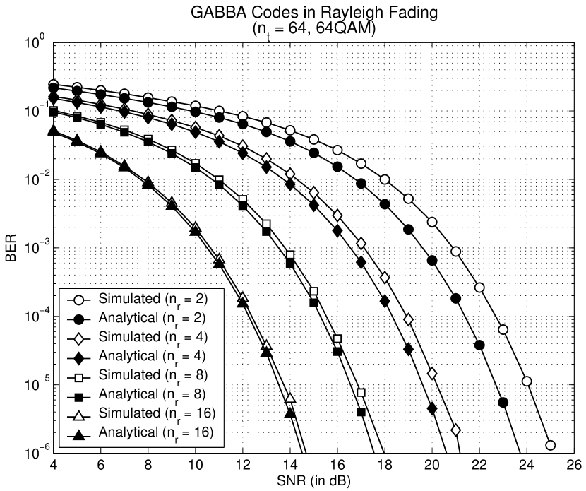
Figure 1: Performance of the GABBA code $\mathbf{C}_{64}$ over $64$-QAM modulation in Rayleigh block-fading channels with various numbers of receive antennas. Simulated results (white markers) were obtained using the orthogonal GABBA decoder described in section IV-C, while analytical results (black markers) were obtained with equation (163), with $\rho=1$ and $\eta=1$ (full-rate full-diversity).

First, in figure 1, the BER performance of a large GABBA code ($n_{t}=64$) simulated over independent and identically distributed (i.i.d.) Rayleigh fading channels is compared against the corresponding analytical BER probability bound. The simulated results (white markers) were obtained with the orthogonal, symbol-by-symbol decoder described in subsection IV-C, while the analytical results (black markers) were computed using equation (163), with $\rho=1$ and $\eta=1$.

A number of important conclusions can be inferred from the comparison. Firstly, the remarkably low complexity of the scheme is emphatically illustrated. Indeed, in order to decode a single block, the ML-decoder, whose performance is associated to the analytical (analytical) curves shown in the figure, would require the minimization of a decision metric over all possible $64$-tuples composed of $64$-QAM constellation symbols, resulting in the prohibitive decoding complexity of $\mathcal{O}(64^{64})$. Likewise, a quasi-orthogonal decoding procedure would require the minimization of two independent decision metrics over all possible $32$-tuples of $64$-QAM symbols, yielding an equally prohibitive decoding complexity of $\mathcal{O}(2\cdot 64^{32})$. In contrast, the proposed orthogonal decoder requires merely the comparison of each orthogonal symbol estimate against the $64$ possible symbols in the constellation, the same complexity of an uncoded system.

Secondly, hard evidence is provided to the fact that the GABBA orthogonal decoder is not a mere zero-forcing technique. This is true because the performance loss of the symbol-by-symbol decoding procedure relative to its bound decreases with the number of receive antennas. In other words, no systematic penalty in signal-to-noise ratio is payed by the use of the GABBA orthogonal decoder. It is difficult to determine exactly the reason why the simulated results obtained with the orthogonal decoder do not match exactly the bounds. The difference between the analytical and simulated curves shown in figure 1 could, in principle, be caused by coloration of noise samples in the decoupled symbol estimates. Since the noise terms at the output of the decoder are linear combinations of the original noise vector, with coefficients given by sum-products of the uncorrelated channel, noise coloration is rather unlikely, especially with large codes and more so when multiple receive antennas are used. This author is led to conclude therefore, that the problem is (even if partly, but substantially) caused by rounding errors inserted by limitations of the simulation platform utilized (in this case Matlab). Anyhow, given the extreme contrast in the complexities involved by each of the alternatives compared, the results shown in figure 1 are nothing but remarkable.

Finally, it is clearly shown that the diversity order attained by the GABBA STBC with its orthogonal decoder is the same as the one theoretically achievable with the ML decoder. This claim is consistent with the discussion of section IV, and is further supported by the results shown in figure 2. In this figure, the simulated and analytical BER probabilities of GABBA codes of various sizes over QPSK modulated signals in the Rayleigh fading channel are compared. It is found that even with a small number of receive antennas ($n_{r}=2$), the performance of orthogonally decoded GABBA codes is close to the theoretical bound, and that the difference between does not increase with the number of transmit antennas $n_{t}$, $i.e.$, as larger codes are used.

V-B2 Unequal Block-fading Channels of Same Statistics

The point of figures 1 and 2 was to illustrate how the GABBA codes and the corresponding orthogonal decoder provide a realistic, high-performing solution for a large, flexible, linear STBC achieving full-rate and full-diversity over i.i.d. fading channels.

Next, we turn our attention to the effects of unequal diversity branches and on the performance of GABBA codes or, in other words, to the effect of utilizing large GABBA codes in the presence of non-i.i.d. fading channels. Our objectives are two-fold, first, to verify that the impact of unequal power and/or unequal statistics of the space-time channels is less significant as the number of transmit antennas increases (larger codes); and, second, to illustrate the flexibility and accuracy of the BER expression given in equation (163).

First, consider the case of channels with the same fading statistics but different powers [46, 47]. This case can be associated to a distributed scenario [12] with cooperative GABBA space-time encoded transmission, where the multiple cooperating transmitters are in the same environment (same channel statistics), but at different locations (different signal strengths at the receiver). The cooperation is assumed to be perfect, $i.e.$, cooperating transmitters are perfectly synchronized and coordinated, such that their transmit signals arrive at the receiver at the same time, at every transmission epoch.

It is also assumed that the average power of each transmit channel is an independent random uniformly distributed in the interval $[0,P_{\textup{max}}]$. Let the average power of the $k$-th transmit channel be denoted by $\bar{p}_{k}$. We start by asking ourselves what is the power distribution profile (across the different transmit channels) that best describes the average scenario faced by the system. Notice that if the statistics of all channels are the same, all diversity branches can, without loss of generality, be relabeled into ascending order. Mathematically we have:

$$\wp_{1}\leq\cdots\leq\wp_{k}\leq\cdots\leq\wp_{K},$$ (166)

The random $\wp_{k}$ is referred to as the $k$-th order statistic of the ensemble $\{\bar{p}_{1},\cdots,\bar{p}_{K}\}$. For $P_{\textup{max}}=1$, the expected value of the $k$-th order statistic $\wp_{k}$ is given by [48, pp. 665, eq. (7.9.20)]

$$\bar{\wp}_{k}=\frac{K!}{(k-1)!(K-k)!}\cdot\int\limits_{0}^{1}{x^{k}\cdot(1-x)^{K-k}dx}.$$ (167)

The integral in equation (167) is a variation of the well-known Beta function [48, pp. 544, eq. (6.12.1)] (a.k.a. Euler’s integral of the first kind), which has no general solution. Fortunately, for $\{k,K\}\in\mathbb{N}$, it is easy to show (see Appendix I) that

$$\int\limits_{0}^{1}{x^{k}\cdot(1-x)^{K-k}dx}=\frac{(K-k)!k!}{(K+1)!}.$$ (168)

From equations (167) and (168), we finally obtain, for a general value of $P_{\textup{max}}$,

$$\bar{\wp}_{k}=\frac{k}{K+1}P_{\textup{max}}.$$ (169)

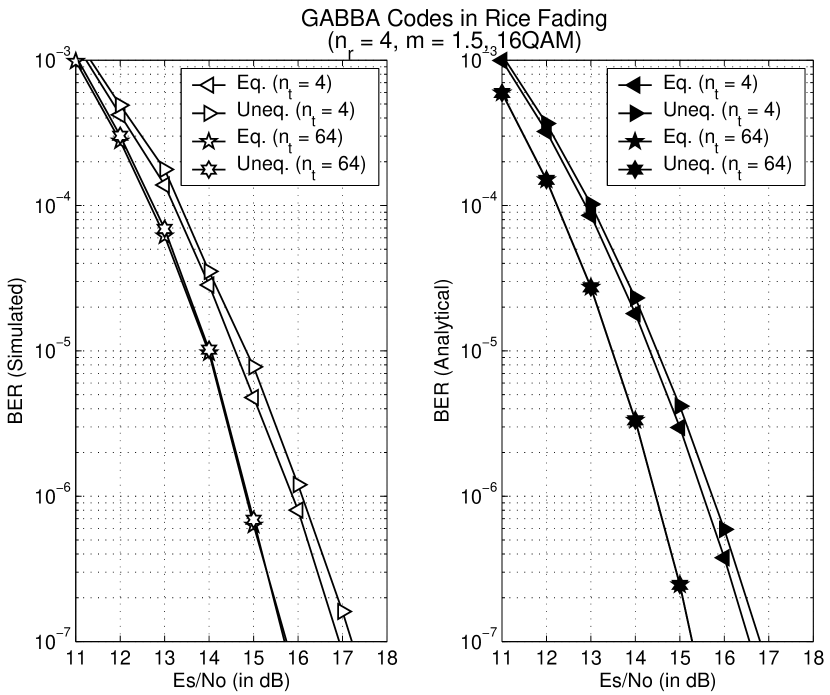
Figure 3: Performance of GABBA codes of different sizes over $16$QAM symbols in Rice block-fading channels with $4$ receive antennas. Simulated results (white markers) were obtained using the orthogonal GABBA decoder described in section IV-C, while analytical results (black markers) were computed using equation (163), with $\rho=1$ and $\eta=1$. Both simulated and analytical results are given for channels with equal and unequal (linear) power distribution profiles across the transmit channels (see section V-B2).

In figure 3, the simulated and analytical performances of GABBA codes of sizes $4$ and $64$, over $16$QAM-modulated symbols in an ensemble of Rice block-fading channels with equal and unequal (linear) power distributions are compared. It can be seen that the impact of an unequal power distribution on the ergodic performance of GABBA-encoded systems loses relevance when large codes are used. As a side product of the comparison, it is once again verified that orthogonally decoded GABBA codes (simulated results) perform very close to the analytical bound (in this case given by equation (163) in combination with equation (158), with $N=K$, $\rho=1$ and $\gamma_{n}=\dfrac{2k}{K}$).

V-B3 Block-fading Channels of Different Statistics

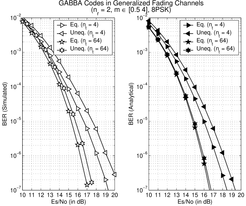
Figure 4: Performance of GABBA codes of different sizes over $8$PSK symbols in generalized block-fading channels with $2$ receive antennas. Simulated results (white markers) were obtained using the orthogonal GABBA decoder described in section IV-C, while analytical results (black markers) were computed using equation (163), with $\rho=1$ and $\eta=1$. Both simulated and analytical results are given for channels with linear power distribution (see section V-B2) and fading severity factors $m$ spanning the interval $[0.5,4]$, as well as equipower channels, and a mean fading severity factor $m=2.5$.

Next, the performances of GABBA codes in uncorrelated block-fading channels with equal and unequal statistics are compared. Results obtained both analytically and through computer simulations are shown in figure 4. The curves corresponding to the unequal fading channels were obtained by assigning to the $k$-th branch a fading severity factor $m_{k}$ and a power factor $\Omega_{k}$ such that $m_{k}$ spans the interval $[0.5,4]$ uniformly, with $m_{k+1}>m_{k}$, while $\sum\Omega_{k}=1$, with $\Omega_{k+1}<\Omega_{k}$. In other words, the channels experiencing more severe fading are also the most powerful ones, such that no particular channel in the ensemble is “dominant”. This distribution of parameters is selected so as to prevent a few channels to dominate the others, ensuring that, instead, all branches have significance in providing diversity. This selection of parameters is associated to scenario faced by peer-to-peer MIMO systems employing diversity-optimized multi-mode adaptive antennas with orthogonal pattern adaptability.

The comparison in figure 4 demonstrates how the use of a large GABBA code results in more robustness against shadowing and other effects that may affect the power distribution and fading statistics of the diversity branches available in peer-to-peer MIMO systems with multi-mode antennas.

The unitary rate and full diversity achieved by GABBA codes ensure that they outperform all (presently known) alternative STBCs of linear construction and comparable complexity (orthogonally decodability). It is, therefore, of little use to show comparisons between GABBA codes and other linear STBCs such as the Alamouti scheme [2], the OSTBC [3, 4], and the maximal-rate minimum-delay (MRMD) codes [22]. The comparison of these codes can, nevertheless, be easily performed analytically utilizing equations (154) and (163), by simply selecting for each technique the corresponding values of $\rho$ (for rate) and $\eta$ (for diversity order).

VI Shannon, and Modulation-Constrained Rate Capacities

In this section, the performance of the proposed GABBA codes is analyzed from a capacity point of view.

The Shannon capacities (over Gaussian constellations) of MIMO systems in ergodic and deterministic fading channels were derived in [16, 30]. More recently, the modulation-constrained rate capacity (maximum average throughput) of MIMO systems over $M$-ary PSK constellations has also been derived [18]. It is known, however, that the rate capacity of linear STBCs (which do not provide multiplexation gain) is bound by the Shannon capacity of the corresponding SIMO channel [17].

It is of interest, therefore, to compare the average throughput theoretically achievable by GABBA codes in systems utilizing different modulation schemes over ensembles of $n_{t}$-by-$n_{r}$ antennas against the ergodic capacity of the equivalent $1$-by-$n_{r}$ SIMO channel. Given the exact BER probability formulae derived in section V-A, a simple yet effective approach at hand is to consider the rate capacity of GABBA codes with hard-decision on the orthogonal symbol estimates. In this case, one can simply considering the binary symmetric channel (as seen from the input of the space-time block encoder up to the output of the corresponding decoder, with the physical MIMO fading channel included), with the transition probabilities given by $\bar{P}_{b}$ and $1-\bar{P}_{b}$, respectively [49]. This leads to

$$C_{{}_{\!M}}(\gamma)=\rho\cdot M\cdot\bigg{[}1+\bar{P}_{b}\cdot\log_{2}\bar{P}_{b}+\left(1\!-\!\bar{P}_{b}\!\right)\cdot\log_{2}\!\left(1\!-\!\bar{P}_{b}\!\right)\bigg{]},$$ (170)

where $\bar{P}_{b}$ is computed with equations (154) or (163), at the given signal-to-noise ratio, considering the corresponding number of transmit and receive antennas $n_{t}$ and $n_{r}$, and with parameters $\rho=1$ and $\eta=1$.

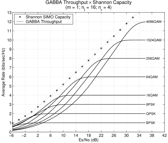
(a) Dominant transmit diversity.

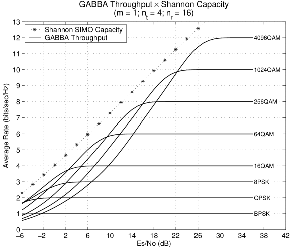
(b) Dominant receive diversity.

Figure 5: Modulation constrained achievable rate (throughput) of GABBA codes of different sizes in Rayleigh fading channel and with different modulation schemes against signal-to-noise ratio.

Using equation (170), the hard-decision modulation-constrained rate capacities of GABBA codes of different sizes, achieved with different modulation schemes, in both dominant transmit ($n_{t}>n_{r}$) and receive ($n_{r}>n_{t}$) diversity scenarios, are compared against the SIMO Shannon capacity in figures 5(a) and 5(b), respectively. It is found that GABBA-encoded systems with optimized modulation comes to roughly $1$ bit/sec/Hz from the Shannon SISO capacity. This is a rather remarkable performance when considered that the Shannon capacity is related to an unfeasible Gaussian modulation and soft-decision decoding. In contrast, the modulation-dependent rates shown for the GABBA scheme can be reached at significantly lower complexities, through concatenation with efficient inner codes such LDPC or Turbo Codes [50], and employing hard decision at the symbol-level. In other words, it is learned from figures 5(a) and 5(b), that the considerably more complex soft-symbol decoding of GABBA codes (concatenated with an inner code) would only improve the rate of the system by $1$ bit/sec/Hz.

It is also noticeable from figures 5(a) and 5(b) that for lower signal-to-noise ratios and relatively lower-order constellations (up to $64$QAM), the GABBA codes considered ($n_{t}=4$ and $n_{t}=16$) actually come to less than $1$ bit/sec/Hz from the Shannon bound. This result is further illustrated in figure 6, where the achievable rates of balanced MIMO systems ($n_{t}=n_{r}$) employing optimum modulation and GABBA codes of different sizes are compared to the corresponding SIMO Shannon capacities. It is interesting to notice that MIMO system with the GABBA scheme and optimum modulation exhibits the same general behavior as the “ideal” Shannon bound when it comes to rate increase in proportion to the number of antennas used in the system.

VII Conclusions

In this paper, a family of linear space-time block codes (STBCs) of unitary rate and full diversity, systematic constructed over arbitrary constellations for any number of transmit antennas are introduced. The codes were obtained from a generalization of the existing ABBA STBCs, a.k.a quasi-orthogonal STBCs (QO-STBCs) and, therefore, are denominated generalized ABBA (GABBA) codes (see section II-B).

It was also shown that the GABBA codes admit fully orthogonal (symbol-by-symbol) decoding. Two key ideas underlie the derivation of the orthogonal GABBA decoder. The first is a transformation applied to the system equation (see section III-A), that exposes the relationship between the code structure and the interference amongst symbols embedded in the same encoding block, characterizing it in terms of an equivalent encoded channel matrix (see section III-B). The second is the exploitation of partition orthogonality properties present in structure of the GABBA codes, which are shown to be transferred to the corresponding encoded channel matrices. It was shown that, as a consequence of these techniques/properties, the received signal vector can decomposed into lower-dimension tuples, each dependent only on certain subsets of the transmitted symbols, via simple linear combinations with coefficients derived directly from the channel estimates. Orthogonal decodability results from the nested application of such linear combinations, with no matrix inversion or iterative signal processing required.

The performance of the proposed GABBA codes were studied both analytically and through computer simulations. The exact BER probability of the codes with ML the decoder over generalized (uncorrelated) fading channels was derived analytically, under the assumption of perfect channel knowledge at the receiver (see section V-A). The formulae were then compared to simulation results obtained with the proposed orthogonal decoder. The comparison reveals that the proposed GABBA solution, despite its very low complexity, achieves nearly the same performance of the bound corresponding to the ML-decoded system, especially in systems with large numbers of antennas (see section V-B).

A brief analysis of the average transmission rate achieved with GABBA codes was also provided. The analysis indicate that the transmission rates achievable with the full(unitary)-rate full-diversity GABBA codes over optimized constellations, with the corresponding orthogonal decoder and hard symbol decision, have the potential to come $1$ bit/sec/Hz from the theoretical bound given by the Shannol SIMO channel capacity. It has been shown that higher rates can be achieved using unitary-rate STBCs as building blocks in a layered structure. Such approaches have already been demonstrated for the known ABBA scheme and OSTBCs [51, Chap. 9], [52, 53]. It is foreseeable, therefore, that these techniques extend naturally to the family of GABBA codes here introduced, with the added flexibility, scalability and low complexity to its advantage.

In addition to the equations, proofs and figures found in the main body of the paper, extensive material is provided in the appendices to allow the verification of all claims, including explicit examples and Matlab implementations of the encoder, the decoder and the BER formulae.

Figure 2: Performance of GABBA codes of different sizes over QPSK symbols in Rayleigh block-fading channels with $2$ receive antennas. Simulated results (white markers) were obtained using the orthogonal GABBA decoder described in section IV-C, while analytical results (black markers) were computed using equation (163), with $\rho=1$ and $\eta=1$ (full-rate full-diversity).

Figure 6: Throughput of GABBA codes against number of transmit and receive antennas ($n_{t}=n_{r}$) in Rayleigh fading channel with optimized modulation.

Appendix A GABBA Encoder

A-A Example: GABBA Mother Encoding Matrix ($K=32$)

$${\scriptstyle\mathbf{C}_{32}=}\!\!\left[\!\!{\tiny\begin{array}[]{rrrrrrrrrrrrrrrrrrrrrrrrrrrrrrrr}&&&&&&&&&&&&&&&\\[0.21529pt] \!\!\!\!s_{1}\!\!\!\!&\!\!\!\!\!\!\!s_{2}\!\!\!\!&\!\!\!\!\!\!\!s_{3}\!\!\!\!&\!\!\!\!\!\!\!s_{4}\!\!\!\!&\!\!\!\!\!\!\!s_{5}\!\!\!\!&\!\!\!\!\!\!\!s_{6}\!\!\!\!&\!\!\!\!\!\!\!s_{7}\!\!\!\!&\!\!\!\!\!\!\!s_{8}\!\!\!\!&\!\!\!\!\!\!\!s_{9}\!\!\!\!&\!\!\!\!\!\!\!s_{10}\!\!\!\!&\!\!\!\!\!\!\!s_{11}\!\!\!\!&\!\!\!\!\!\!\!s_{12}\!\!\!\!&\!\!\!\!\!\!\!s_{13}\!\!\!\!&\!\!\!\!\!\!\!s_{14}\!\!\!\!&\!\!\!\!\!\!\!s_{15}\!\!\!\!&\!\!\!\!\!\!\!s_{16}\!\!\!\!&\!\!\!\!\!\!\!s_{17}\!\!\!\!&\!\!\!\!\!\!\!s_{18}\!\!\!\!&\!\!\!\!\!\!\!s_{19}\!\!\!\!&\!\!\!\!\!\!\!s_{20}\!\!\!\!&\!\!\!\!\!\!\!s_{21}\!\!\!\!&\!\!\!\!\!\!\!s_{22}\!\!\!\!&\!\!\!\!\!\!\!s_{23}\!\!\!\!&\!\!\!\!\!\!\!s_{24}\!\!\!\!&\!\!\!\!\!\!\!s_{25}\!\!\!\!&\!\!\!\!\!\!\!s_{26}\!\!\!\!&\!\!\!\!\!\!\!s_{27}\!\!\!\!&\!\!\!\!\!\!\!s_{28}\!\!\!\!&\!\!\!\!\!\!\!s_{29}\!\!\!\!&\!\!\!\!\!\!\!s_{30}\!\!\!\!&\!\!\!\!\!\!\!s_{31}\!\!\!\!&\!\!\!\!\!\!\!s_{32}\\ \!\!-\!\!s_{2}\!\!\!\!&\!\!\!\!\!\!\!s_{1}\!\!\!\!&\!\!\!\!\!-\!\!s_{4}\!\!\!\!&\!\!\!\!\!\!\!s_{3}\!\!\!\!&\!\!\!\!\!-\!\!s_{6}\!\!\!\!&\!\!\!\!\!\!\!s_{5}\!\!\!\!&\!\!\!\!\!-\!\!s_{8}\!\!\!\!&\!\!\!\!\!\!\!s_{7}\!\!\!\!&\!\!\!\!\!-\!\!s_{10}\!\!\!\!&\!\!\!\!\!\!\!s_{9}\!\!\!\!&\!\!\!\!\!-\!\!s_{12}\!\!\!\!&\!\!\!\!\!\!\!s_{11}\!\!\!\!&\!\!\!\!\!-\!\!s_{14}\!\!\!\!&\!\!\!\!\!\!\!s_{13}\!\!\!\!&\!\!\!\!\!-\!\!s_{16}\!\!\!\!&\!\!\!\!\!\!\!s_{15}\!\!\!\!&\!\!\!\!\!-\!\!s_{18}\!\!\!\!&\!\!\!\!\!\!\!s_{17}\!\!\!\!&\!\!\!\!\!-\!\!s_{20}\!\!\!\!&\!\!\!\!\!\!\!s_{19}\!\!\!\!&\!\!\!\!\!-\!\!s_{22}\!\!\!\!&\!\!\!\!\!\!\!s_{21}\!\!\!\!&\!\!\!\!\!-\!\!s_{24}\!\!\!\!&\!\!\!\!\!\!\!s_{23}\!\!\!\!&\!\!\!\!\!-\!\!s_{26}\!\!\!\!&\!\!\!\!\!\!\!s_{25}\!\!\!\!&\!\!\!\!\!-\!\!s_{28}\!\!\!\!&\!\!\!\!\!\!\!s_{27}\!\!\!\!&\!\!\!\!\!-\!\!s_{30}\!\!\!\!&\!\!\!\!\!\!\!s_{29}\!\!\!\!&\!\!\!\!\!-\!\!s_{32}\!\!\!\!&\!\!\!\!\!\!\!s_{31}\\ \!\!-\!\!s_{3}\!\!\!\!&\!\!\!\!\!-\!\!s_{4}\!\!\!\!&\!\!\!\!\!\!\!s_{1}\!\!\!\!&\!\!\!\!\!\!\!s_{2}\!\!\!\!&\!\!\!\!\!-\!\!s_{7}\!\!\!\!&\!\!\!\!\!-\!\!s_{8}\!\!\!\!&\!\!\!\!\!\!\!s_{5}\!\!\!\!&\!\!\!\!\!\!\!s_{6}\!\!\!\!&\!\!\!\!\!-\!\!s_{11}\!\!\!\!&\!\!\!\!\!-\!\!s_{12}\!\!\!\!&\!\!\!\!\!\!\!s_{9}\!\!\!\!&\!\!\!\!\!\!\!s_{10}\!\!\!\!&\!\!\!\!\!-\!\!s_{15}\!\!\!\!&\!\!\!\!\!-\!\!s_{16}\!\!\!\!&\!\!\!\!\!\!\!s_{13}\!\!\!\!&\!\!\!\!\!\!\!s_{14}\!\!\!\!&\!\!\!\!\!-\!\!s_{19}\!\!\!\!&\!\!\!\!\!-\!\!s_{20}\!\!\!\!&\!\!\!\!\!\!\!s_{17}\!\!\!\!&\!\!\!\!\!\!\!s_{18}\!\!\!\!&\!\!\!\!\!-\!\!s_{23}\!\!\!\!&\!\!\!\!\!-\!\!s_{24}\!\!\!\!&\!\!\!\!\!\!\!s_{21}\!\!\!\!&\!\!\!\!\!\!\!s_{22}\!\!\!\!&\!\!\!\!\!-\!\!s_{27}\!\!\!\!&\!\!\!\!\!-\!\!s_{28}\!\!\!\!&\!\!\!\!\!\!\!s_{25}\!\!\!\!&\!\!\!\!\!\!\!s_{26}\!\!\!\!&\!\!\!\!\!-\!\!s_{31}\!\!\!\!&\!\!\!\!\!-\!\!s_{32}\!\!\!\!&\!\!\!\!\!\!\!s_{29}\!\!\!\!&\!\!\!\!\!\!\!s_{30}\\ \!\!\!\!s_{4}\!\!\!\!&\!\!\!\!\!-\!\!s_{3}\!\!\!\!&\!\!\!\!\!-\!\!s_{2}\!\!\!\!&\!\!\!\!\!\!\!s_{1}\!\!\!\!&\!\!\!\!\!\!\!s_{8}\!\!\!\!&\!\!\!\!\!-\!\!s_{7}\!\!\!\!&\!\!\!\!\!-\!\!s_{6}\!\!\!\!&\!\!\!\!\!\!\!s_{5}\!\!\!\!&\!\!\!\!\!\!\!s_{12}\!\!\!\!&\!\!\!\!\!-\!\!s_{11}\!\!\!\!&\!\!\!\!\!-\!\!s_{10}\!\!\!\!&\!\!\!\!\!\!\!s_{9}\!\!\!\!&\!\!\!\!\!\!\!s_{16}\!\!\!\!&\!\!\!\!\!-\!\!s_{15}\!\!\!\!&\!\!\!\!\!-\!\!s_{14}\!\!\!\!&\!\!\!\!\!\!\!s_{13}\!\!\!\!&\!\!\!\!\!\!\!s_{20}\!\!\!\!&\!\!\!\!\!-\!\!s_{19}\!\!\!\!&\!\!\!\!\!-\!\!s_{18}\!\!\!\!&\!\!\!\!\!\!\!s_{17}\!\!\!\!&\!\!\!\!\!\!\!s_{24}\!\!\!\!&\!\!\!\!\!-\!\!s_{23}\!\!\!\!&\!\!\!\!\!-\!\!s_{22}\!\!\!\!&\!\!\!\!\!\!\!s_{21}\!\!\!\!&\!\!\!\!\!\!\!s_{28}\!\!\!\!&\!\!\!\!\!-\!\!s_{27}\!\!\!\!&\!\!\!\!\!-\!\!s_{26}\!\!\!\!&\!\!\!\!\!\!\!s_{25}\!\!\!\!&\!\!\!\!\!\!\!s_{32}\!\!\!\!&\!\!\!\!\!-\!\!s_{31}\!\!\!\!&\!\!\!\!\!-\!\!s_{30}\!\!\!\!&\!\!\!\!\!\!\!s_{29}\\ \!\!-\!\!s_{5}\!\!\!\!&\!\!\!\!\!-\!\!s_{6}\!\!\!\!&\!\!\!\!\!-\!\!s_{7}\!\!\!\!&\!\!\!\!\!-\!\!s_{8}\!\!\!\!&\!\!\!\!\!\!\!s_{1}\!\!\!\!&\!\!\!\!\!\!\!s_{2}\!\!\!\!&\!\!\!\!\!\!\!s_{3}\!\!\!\!&\!\!\!\!\!\!\!s_{4}\!\!\!\!&\!\!\!\!\!-\!\!s_{13}\!\!\!\!&\!\!\!\!\!-\!\!s_{14}\!\!\!\!&\!\!\!\!\!-\!\!s_{15}\!\!\!\!&\!\!\!\!\!-\!\!s_{16}\!\!\!\!&\!\!\!\!\!\!\!s_{9}\!\!\!\!&\!\!\!\!\!\!\!s_{10}\!\!\!\!&\!\!\!\!\!\!\!s_{11}\!\!\!\!&\!\!\!\!\!\!\!s_{12}\!\!\!\!&\!\!\!\!\!-\!\!s_{21}\!\!\!\!&\!\!\!\!\!-\!\!s_{22}\!\!\!\!&\!\!\!\!\!-\!\!s_{23}\!\!\!\!&\!\!\!\!\!-\!\!s_{24}\!\!\!\!&\!\!\!\!\!\!\!s_{17}\!\!\!\!&\!\!\!\!\!\!\!s_{18}\!\!\!\!&\!\!\!\!\!\!\!s_{19}\!\!\!\!&\!\!\!\!\!\!\!s_{20}\!\!\!\!&\!\!\!\!\!-\!\!s_{29}\!\!\!\!&\!\!\!\!\!-\!\!s_{30}\!\!\!\!&\!\!\!\!\!-\!\!s_{31}\!\!\!\!&\!\!\!\!\!-\!\!s_{32}\!\!\!\!&\!\!\!\!\!\!\!s_{25}\!\!\!\!&\!\!\!\!\!\!\!s_{26}\!\!\!\!&\!\!\!\!\!\!\!s_{27}\!\!\!\!&\!\!\!\!\!\!\!s_{28}\\ \!\!\!\!s_{6}\!\!\!\!&\!\!\!\!\!-\!\!s_{5}\!\!\!\!&\!\!\!\!\!\!\!s_{8}\!\!\!\!&\!\!\!\!\!-\!\!s_{7}\!\!\!\!&\!\!\!\!\!-\!\!s_{2}\!\!\!\!&\!\!\!\!\!\!\!s_{1}\!\!\!\!&\!\!\!\!\!-\!\!s_{4}\!\!\!\!&\!\!\!\!\!\!\!s_{3}\!\!\!\!&\!\!\!\!\!\!\!s_{14}\!\!\!\!&\!\!\!\!\!-\!\!s_{13}\!\!\!\!&\!\!\!\!\!\!\!s_{16}\!\!\!\!&\!\!\!\!\!-\!\!s_{15}\!\!\!\!&\!\!\!\!\!-\!\!s_{10}\!\!\!\!&\!\!\!\!\!\!\!s_{9}\!\!\!\!&\!\!\!\!\!-\!\!s_{12}\!\!\!\!&\!\!\!\!\!\!\!s_{11}\!\!\!\!&\!\!\!\!\!\!\!s_{22}\!\!\!\!&\!\!\!\!\!-\!\!s_{21}\!\!\!\!&\!\!\!\!\!\!\!s_{24}\!\!\!\!&\!\!\!\!\!-\!\!s_{23}\!\!\!\!&\!\!\!\!\!-\!\!s_{18}\!\!\!\!&\!\!\!\!\!\!\!s_{17}\!\!\!\!&\!\!\!\!\!-\!\!s_{20}\!\!\!\!&\!\!\!\!\!\!\!s_{19}\!\!\!\!&\!\!\!\!\!\!\!s_{30}\!\!\!\!&\!\!\!\!\!-\!\!s_{29}\!\!\!\!&\!\!\!\!\!\!\!s_{32}\!\!\!\!&\!\!\!\!\!-\!\!s_{31}\!\!\!\!&\!\!\!\!\!-\!\!s_{26}\!\!\!\!&\!\!\!\!\!\!\!s_{25}\!\!\!\!&\!\!\!\!\!-\!\!s_{28}\!\!\!\!&\!\!\!\!\!\!\!s_{27}\\ \!\!\!\!s_{7}\!\!\!\!&\!\!\!\!\!\!\!s_{8}\!\!\!\!&\!\!\!\!\!-\!\!s_{5}\!\!\!\!&\!\!\!\!\!-\!\!s_{6}\!\!\!\!&\!\!\!\!\!-\!\!s_{3}\!\!\!\!&\!\!\!\!\!-\!\!s_{4}\!\!\!\!&\!\!\!\!\!\!\!s_{1}\!\!\!\!&\!\!\!\!\!\!\!s_{2}\!\!\!\!&\!\!\!\!\!\!\!s_{15}\!\!\!\!&\!\!\!\!\!\!\!s_{16}\!\!\!\!&\!\!\!\!\!-\!\!s_{13}\!\!\!\!&\!\!\!\!\!-\!\!s_{14}\!\!\!\!&\!\!\!\!\!-\!\!s_{11}\!\!\!\!&\!\!\!\!\!-\!\!s_{12}\!\!\!\!&\!\!\!\!\!\!\!s_{9}\!\!\!\!&\!\!\!\!\!\!\!s_{10}\!\!\!\!&\!\!\!\!\!\!\!s_{23}\!\!\!\!&\!\!\!\!\!\!\!s_{24}\!\!\!\!&\!\!\!\!\!-\!\!s_{21}\!\!\!\!&\!\!\!\!\!-\!\!s_{22}\!\!\!\!&\!\!\!\!\!-\!\!s_{19}\!\!\!\!&\!\!\!\!\!-\!\!s_{20}\!\!\!\!&\!\!\!\!\!\!\!s_{17}\!\!\!\!&\!\!\!\!\!\!\!s_{18}\!\!\!\!&\!\!\!\!\!\!\!s_{31}\!\!\!\!&\!\!\!\!\!\!\!s_{32}\!\!\!\!&\!\!\!\!\!-\!\!s_{29}\!\!\!\!&\!\!\!\!\!-\!\!s_{30}\!\!\!\!&\!\!\!\!\!-\!\!s_{27}\!\!\!\!&\!\!\!\!\!-\!\!s_{28}\!\!\!\!&\!\!\!\!\!\!\!s_{25}\!\!\!\!&\!\!\!\!\!\!\!s_{26}\\ \!\!-\!\!s_{8}\!\!\!\!&\!\!\!\!\!\!\!s_{7}\!\!\!\!&\!\!\!\!\!\!\!s_{6}\!\!\!\!&\!\!\!\!\!-\!\!s_{5}\!\!\!\!&\!\!\!\!\!\!\!s_{4}\!\!\!\!&\!\!\!\!\!-\!\!s_{3}\!\!\!\!&\!\!\!\!\!-\!\!s_{2}\!\!\!\!&\!\!\!\!\!\!\!s_{1}\!\!\!\!&\!\!\!\!\!-\!\!s_{16}\!\!\!\!&\!\!\!\!\!\!\!s_{15}\!\!\!\!&\!\!\!\!\!\!\!s_{14}\!\!\!\!&\!\!\!\!\!-\!\!s_{13}\!\!\!\!&\!\!\!\!\!\!\!s_{12}\!\!\!\!&\!\!\!\!\!-\!\!s_{11}\!\!\!\!&\!\!\!\!\!-\!\!s_{10}\!\!\!\!&\!\!\!\!\!\!\!s_{9}\!\!\!\!&\!\!\!\!\!-\!\!s_{24}\!\!\!\!&\!\!\!\!\!\!\!s_{23}\!\!\!\!&\!\!\!\!\!\!\!s_{22}\!\!\!\!&\!\!\!\!\!-\!\!s_{21}\!\!\!\!&\!\!\!\!\!\!\!s_{20}\!\!\!\!&\!\!\!\!\!-\!\!s_{19}\!\!\!\!&\!\!\!\!\!-\!\!s_{18}\!\!\!\!&\!\!\!\!\!\!\!s_{17}\!\!\!\!&\!\!\!\!\!-\!\!s_{32}\!\!\!\!&\!\!\!\!\!\!\!s_{31}\!\!\!\!&\!\!\!\!\!\!\!s_{30}\!\!\!\!&\!\!\!\!\!-\!\!s_{29}\!\!\!\!&\!\!\!\!\!\!\!s_{28}\!\!\!\!&\!\!\!\!\!-\!\!s_{27}\!\!\!\!&\!\!\!\!\!-\!\!s_{26}\!\!\!\!&\!\!\!\!\!\!\!s_{25}\\ \!\!-\!\!s_{9}\!\!\!\!&\!\!\!\!\!-\!\!s_{10}\!\!\!\!&\!\!\!\!\!-\!\!s_{11}\!\!\!\!&\!\!\!\!\!-\!\!s_{12}\!\!\!\!&\!\!\!\!\!-\!\!s_{13}\!\!\!\!&\!\!\!\!\!-\!\!s_{14}\!\!\!\!&\!\!\!\!\!-\!\!s_{15}\!\!\!\!&\!\!\!\!\!-\!\!s_{16}\!\!\!\!&\!\!\!\!\!\!\!s_{1}\!\!\!\!&\!\!\!\!\!\!\!s_{2}\!\!\!\!&\!\!\!\!\!\!\!s_{3}\!\!\!\!&\!\!\!\!\!\!\!s_{4}\!\!\!\!&\!\!\!\!\!\!\!s_{5}\!\!\!\!&\!\!\!\!\!\!\!s_{6}\!\!\!\!&\!\!\!\!\!\!\!s_{7}\!\!\!\!&\!\!\!\!\!\!\!s_{8}\!\!\!\!&\!\!\!\!\!-\!\!s_{25}\!\!\!\!&\!\!\!\!\!-\!\!s_{26}\!\!\!\!&\!\!\!\!\!-\!\!s_{27}\!\!\!\!&\!\!\!\!\!-\!\!s_{28}\!\!\!\!&\!\!\!\!\!-\!\!s_{29}\!\!\!\!&\!\!\!\!\!-\!\!s_{30}\!\!\!\!&\!\!\!\!\!-\!\!s_{31}\!\!\!\!&\!\!\!\!\!-\!\!s_{32}\!\!\!\!&\!\!\!\!\!\!\!s_{17}\!\!\!\!&\!\!\!\!\!\!\!s_{18}\!\!\!\!&\!\!\!\!\!\!\!s_{19}\!\!\!\!&\!\!\!\!\!\!\!s_{20}\!\!\!\!&\!\!\!\!\!\!\!s_{21}\!\!\!\!&\!\!\!\!\!\!\!s_{22}\!\!\!\!&\!\!\!\!\!\!\!s_{23}\!\!\!\!&\!\!\!\!\!\!\!s_{24}\\ \!\!\!\!s_{10}\!\!\!\!&\!\!\!\!\!-\!\!s_{9}\!\!\!\!&\!\!\!\!\!\!\!s_{12}\!\!\!\!&\!\!\!\!\!-\!\!s_{11}\!\!\!\!&\!\!\!\!\!\!\!s_{14}\!\!\!\!&\!\!\!\!\!-\!\!s_{13}\!\!\!\!&\!\!\!\!\!\!\!s_{16}\!\!\!\!&\!\!\!\!\!-\!\!s_{15}\!\!\!\!&\!\!\!\!\!-\!\!s_{2}\!\!\!\!&\!\!\!\!\!\!\!s_{1}\!\!\!\!&\!\!\!\!\!-\!\!s_{4}\!\!\!\!&\!\!\!\!\!\!\!s_{3}\!\!\!\!&\!\!\!\!\!-\!\!s_{6}\!\!\!\!&\!\!\!\!\!\!\!s_{5}\!\!\!\!&\!\!\!\!\!-\!\!s_{8}\!\!\!\!&\!\!\!\!\!\!\!s_{7}\!\!\!\!&\!\!\!\!\!\!\!s_{26}\!\!\!\!&\!\!\!\!\!-\!\!s_{25}\!\!\!\!&\!\!\!\!\!\!\!s_{28}\!\!\!\!&\!\!\!\!\!-\!\!s_{27}\!\!\!\!&\!\!\!\!\!\!\!s_{30}\!\!\!\!&\!\!\!\!\!-\!\!s_{29}\!\!\!\!&\!\!\!\!\!\!\!s_{32}\!\!\!\!&\!\!\!\!\!-\!\!s_{31}\!\!\!\!&\!\!\!\!\!-\!\!s_{18}\!\!\!\!&\!\!\!\!\!\!\!s_{17}\!\!\!\!&\!\!\!\!\!-\!\!s_{20}\!\!\!\!&\!\!\!\!\!\!\!s_{19}\!\!\!\!&\!\!\!\!\!-\!\!s_{22}\!\!\!\!&\!\!\!\!\!\!\!s_{21}\!\!\!\!&\!\!\!\!\!-\!\!s_{24}\!\!\!\!&\!\!\!\!\!\!\!s_{23}\\ \!\!\!\!s_{11}\!\!\!\!&\!\!\!\!\!\!\!s_{12}\!\!\!\!&\!\!\!\!\!-\!\!s_{9}\!\!\!\!&\!\!\!\!\!-\!\!s_{10}\!\!\!\!&\!\!\!\!\!\!\!s_{15}\!\!\!\!&\!\!\!\!\!\!\!s_{16}\!\!\!\!&\!\!\!\!\!-\!\!s_{13}\!\!\!\!&\!\!\!\!\!-\!\!s_{14}\!\!\!\!&\!\!\!\!\!-\!\!s_{3}\!\!\!\!&\!\!\!\!\!-\!\!s_{4}\!\!\!\!&\!\!\!\!\!\!\!s_{1}\!\!\!\!&\!\!\!\!\!\!\!s_{2}\!\!\!\!&\!\!\!\!\!-\!\!s_{7}\!\!\!\!&\!\!\!\!\!-\!\!s_{8}\!\!\!\!&\!\!\!\!\!\!\!s_{5}\!\!\!\!&\!\!\!\!\!\!\!s_{6}\!\!\!\!&\!\!\!\!\!\!\!s_{27}\!\!\!\!&\!\!\!\!\!\!\!s_{28}\!\!\!\!&\!\!\!\!\!-\!\!s_{25}\!\!\!\!&\!\!\!\!\!-\!\!s_{26}\!\!\!\!&\!\!\!\!\!\!\!s_{31}\!\!\!\!&\!\!\!\!\!\!\!s_{32}\!\!\!\!&\!\!\!\!\!-\!\!s_{29}\!\!\!\!&\!\!\!\!\!-\!\!s_{30}\!\!\!\!&\!\!\!\!\!-\!\!s_{19}\!\!\!\!&\!\!\!\!\!-\!\!s_{20}\!\!\!\!&\!\!\!\!\!\!\!s_{17}\!\!\!\!&\!\!\!\!\!\!\!s_{18}\!\!\!\!&\!\!\!\!\!-\!\!s_{23}\!\!\!\!&\!\!\!\!\!-\!\!s_{24}\!\!\!\!&\!\!\!\!\!\!\!s_{21}\!\!\!\!&\!\!\!\!\!\!\!s_{22}\\ \!\!-\!\!s_{12}\!\!\!\!&\!\!\!\!\!\!\!s_{11}\!\!\!\!&\!\!\!\!\!\!\!s_{10}\!\!\!\!&\!\!\!\!\!-\!\!s_{9}\!\!\!\!&\!\!\!\!\!-\!\!s_{16}\!\!\!\!&\!\!\!\!\!\!\!s_{15}\!\!\!\!&\!\!\!\!\!\!\!s_{14}\!\!\!\!&\!\!\!\!\!-\!\!s_{13}\!\!\!\!&\!\!\!\!\!\!\!s_{4}\!\!\!\!&\!\!\!\!\!-\!\!s_{3}\!\!\!\!&\!\!\!\!\!-\!\!s_{2}\!\!\!\!&\!\!\!\!\!\!\!s_{1}\!\!\!\!&\!\!\!\!\!\!\!s_{8}\!\!\!\!&\!\!\!\!\!-\!\!s_{7}\!\!\!\!&\!\!\!\!\!-\!\!s_{6}\!\!\!\!&\!\!\!\!\!\!\!s_{5}\!\!\!\!&\!\!\!\!\!-\!\!s_{28}\!\!\!\!&\!\!\!\!\!\!\!s_{27}\!\!\!\!&\!\!\!\!\!\!\!s_{26}\!\!\!\!&\!\!\!\!\!-\!\!s_{25}\!\!\!\!&\!\!\!\!\!-\!\!s_{32}\!\!\!\!&\!\!\!\!\!\!\!s_{31}\!\!\!\!&\!\!\!\!\!\!\!s_{30}\!\!\!\!&\!\!\!\!\!-\!\!s_{29}\!\!\!\!&\!\!\!\!\!\!\!s_{20}\!\!\!\!&\!\!\!\!\!-\!\!s_{19}\!\!\!\!&\!\!\!\!\!-\!\!s_{18}\!\!\!\!&\!\!\!\!\!\!\!s_{17}\!\!\!\!&\!\!\!\!\!\!\!s_{24}\!\!\!\!&\!\!\!\!\!-\!\!s_{23}\!\!\!\!&\!\!\!\!\!-\!\!s_{22}\!\!\!\!&\!\!\!\!\!\!\!s_{21}\\ \!\!\!\!s_{13}\!\!\!\!&\!\!\!\!\!\!\!s_{14}\!\!\!\!&\!\!\!\!\!\!\!s_{15}\!\!\!\!&\!\!\!\!\!\!\!s_{16}\!\!\!\!&\!\!\!\!\!-\!\!s_{9}\!\!\!\!&\!\!\!\!\!-\!\!s_{10}\!\!\!\!&\!\!\!\!\!-\!\!s_{11}\!\!\!\!&\!\!\!\!\!-\!\!s_{12}\!\!\!\!&\!\!\!\!\!-\!\!s_{5}\!\!\!\!&\!\!\!\!\!-\!\!s_{6}\!\!\!\!&\!\!\!\!\!-\!\!s_{7}\!\!\!\!&\!\!\!\!\!-\!\!s_{8}\!\!\!\!&\!\!\!\!\!\!\!s_{1}\!\!\!\!&\!\!\!\!\!\!\!s_{2}\!\!\!\!&\!\!\!\!\!\!\!s_{3}\!\!\!\!&\!\!\!\!\!\!\!s_{4}\!\!\!\!&\!\!\!\!\!\!\!s_{29}\!\!\!\!&\!\!\!\!\!\!\!s_{30}\!\!\!\!&\!\!\!\!\!\!\!s_{31}\!\!\!\!&\!\!\!\!\!\!\!s_{32}\!\!\!\!&\!\!\!\!\!-\!\!s_{25}\!\!\!\!&\!\!\!\!\!-\!\!s_{26}\!\!\!\!&\!\!\!\!\!-\!\!s_{27}\!\!\!\!&\!\!\!\!\!-\!\!s_{28}\!\!\!\!&\!\!\!\!\!-\!\!s_{21}\!\!\!\!&\!\!\!\!\!-\!\!s_{22}\!\!\!\!&\!\!\!\!\!-\!\!s_{23}\!\!\!\!&\!\!\!\!\!-\!\!s_{24}\!\!\!\!&\!\!\!\!\!\!\!s_{17}\!\!\!\!&\!\!\!\!\!\!\!s_{18}\!\!\!\!&\!\!\!\!\!\!\!s_{19}\!\!\!\!&\!\!\!\!\!\!\!s_{20}\\ \!\!-\!\!s_{14}\!\!\!\!&\!\!\!\!\!\!\!s_{13}\!\!\!\!&\!\!\!\!\!-\!\!s_{16}\!\!\!\!&\!\!\!\!\!\!\!s_{15}\!\!\!\!&\!\!\!\!\!\!\!s_{10}\!\!\!\!&\!\!\!\!\!-\!\!s_{9}\!\!\!\!&\!\!\!\!\!\!\!s_{12}\!\!\!\!&\!\!\!\!\!-\!\!s_{11}\!\!\!\!&\!\!\!\!\!\!\!s_{6}\!\!\!\!&\!\!\!\!\!-\!\!s_{5}\!\!\!\!&\!\!\!\!\!\!\!s_{8}\!\!\!\!&\!\!\!\!\!-\!\!s_{7}\!\!\!\!&\!\!\!\!\!-\!\!s_{2}\!\!\!\!&\!\!\!\!\!\!\!s_{1}\!\!\!\!&\!\!\!\!\!-\!\!s_{4}\!\!\!\!&\!\!\!\!\!\!\!s_{3}\!\!\!\!&\!\!\!\!\!-\!\!s_{30}\!\!\!\!&\!\!\!\!\!\!\!s_{29}\!\!\!\!&\!\!\!\!\!-\!\!s_{32}\!\!\!\!&\!\!\!\!\!\!\!s_{31}\!\!\!\!&\!\!\!\!\!\!\!s_{26}\!\!\!\!&\!\!\!\!\!-\!\!s_{25}\!\!\!\!&\!\!\!\!\!\!\!s_{28}\!\!\!\!&\!\!\!\!\!-\!\!s_{27}\!\!\!\!&\!\!\!\!\!\!\!s_{22}\!\!\!\!&\!\!\!\!\!-\!\!s_{21}\!\!\!\!&\!\!\!\!\!\!\!s_{24}\!\!\!\!&\!\!\!\!\!-\!\!s_{23}\!\!\!\!&\!\!\!\!\!-\!\!s_{18}\!\!\!\!&\!\!\!\!\!\!\!s_{17}\!\!\!\!&\!\!\!\!\!-\!\!s_{20}\!\!\!\!&\!\!\!\!\!\!\!s_{19}\\ \!\!-\!\!s_{15}\!\!\!\!&\!\!\!\!\!-\!\!s_{16}\!\!\!\!&\!\!\!\!\!\!\!s_{13}\!\!\!\!&\!\!\!\!\!\!\!s_{14}\!\!\!\!&\!\!\!\!\!\!\!s_{11}\!\!\!\!&\!\!\!\!\!\!\!s_{12}\!\!\!\!&\!\!\!\!\!-\!\!s_{9}\!\!\!\!&\!\!\!\!\!-\!\!s_{10}\!\!\!\!&\!\!\!\!\!\!\!s_{7}\!\!\!\!&\!\!\!\!\!\!\!s_{8}\!\!\!\!&\!\!\!\!\!-\!\!s_{5}\!\!\!\!&\!\!\!\!\!-\!\!s_{6}\!\!\!\!&\!\!\!\!\!-\!\!s_{3}\!\!\!\!&\!\!\!\!\!-\!\!s_{4}\!\!\!\!&\!\!\!\!\!\!\!s_{1}\!\!\!\!&\!\!\!\!\!\!\!s_{2}\!\!\!\!&\!\!\!\!\!-\!\!s_{31}\!\!\!\!&\!\!\!\!\!-\!\!s_{32}\!\!\!\!&\!\!\!\!\!\!\!s_{29}\!\!\!\!&\!\!\!\!\!\!\!s_{30}\!\!\!\!&\!\!\!\!\!\!\!s_{27}\!\!\!\!&\!\!\!\!\!\!\!s_{28}\!\!\!\!&\!\!\!\!\!-\!\!s_{25}\!\!\!\!&\!\!\!\!\!-\!\!s_{26}\!\!\!\!&\!\!\!\!\!\!\!s_{23}\!\!\!\!&\!\!\!\!\!\!\!s_{24}\!\!\!\!&\!\!\!\!\!-\!\!s_{21}\!\!\!\!&\!\!\!\!\!-\!\!s_{22}\!\!\!\!&\!\!\!\!\!-\!\!s_{19}\!\!\!\!&\!\!\!\!\!-\!\!s_{20}\!\!\!\!&\!\!\!\!\!\!\!s_{17}\!\!\!\!&\!\!\!\!\!\!\!s_{18}\\ \!\!\!\!s_{16}\!\!\!\!&\!\!\!\!\!-\!\!s_{15}\!\!\!\!&\!\!\!\!\!-\!\!s_{14}\!\!\!\!&\!\!\!\!\!\!\!s_{13}\!\!\!\!&\!\!\!\!\!-\!\!s_{12}\!\!\!\!&\!\!\!\!\!\!\!s_{11}\!\!\!\!&\!\!\!\!\!\!\!s_{10}\!\!\!\!&\!\!\!\!\!-\!\!s_{9}\!\!\!\!&\!\!\!\!\!-\!\!s_{8}\!\!\!\!&\!\!\!\!\!\!\!s_{7}\!\!\!\!&\!\!\!\!\!\!\!s_{6}\!\!\!\!&\!\!\!\!\!-\!\!s_{5}\!\!\!\!&\!\!\!\!\!\!\!s_{4}\!\!\!\!&\!\!\!\!\!-\!\!s_{3}\!\!\!\!&\!\!\!\!\!-\!\!s_{2}\!\!\!\!&\!\!\!\!\!\!\!s_{1}\!\!\!\!&\!\!\!\!\!\!\!s_{32}\!\!\!\!&\!\!\!\!\!-\!\!s_{31}\!\!\!\!&\!\!\!\!\!-\!\!s_{30}\!\!\!\!&\!\!\!\!\!\!\!s_{29}\!\!\!\!&\!\!\!\!\!-\!\!s_{28}\!\!\!\!&\!\!\!\!\!\!\!s_{27}\!\!\!\!&\!\!\!\!\!\!\!s_{26}\!\!\!\!&\!\!\!\!\!-\!\!s_{25}\!\!\!\!&\!\!\!\!\!-\!\!s_{24}\!\!\!\!&\!\!\!\!\!\!\!s_{23}\!\!\!\!&\!\!\!\!\!\!\!s_{22}\!\!\!\!&\!\!\!\!\!-\!\!s_{21}\!\!\!\!&\!\!\!\!\!\!\!s_{20}\!\!\!\!&\!\!\!\!\!-\!\!s_{19}\!\!\!\!&\!\!\!\!\!-\!\!s_{18}\!\!\!\!&\!\!\!\!\!\!\!s_{17}\\ \!\!-\!\!s_{17}^{*}\!\!\!\!&\!\!\!\!\!\!\!s_{18}^{*}\!\!\!\!&\!\!\!\!\!\!\!s_{19}^{*}\!\!\!\!&\!\!\!\!\!-\!\!s_{20}^{*}\!\!\!\!&\!\!\!\!\!\!\!s_{21}^{*}\!\!\!\!&\!\!\!\!\!-\!\!s_{22}^{*}\!\!\!\!&\!\!\!\!\!-\!\!s_{23}^{*}\!\!\!\!&\!\!\!\!\!\!\!s_{24}^{*}\!\!\!\!&\!\!\!\!\!\!\!s_{25}^{*}\!\!\!\!&\!\!\!\!\!-\!\!s_{26}^{*}\!\!\!\!&\!\!\!\!\!-\!\!s_{27}^{*}\!\!\!\!&\!\!\!\!\!\!\!s_{28}^{*}\!\!\!\!&\!\!\!\!\!-\!\!s_{29}^{*}\!\!\!\!&\!\!\!\!\!\!\!s_{30}^{*}\!\!\!\!&\!\!\!\!\!\!\!s_{31}^{*}\!\!\!\!&\!\!\!\!\!-\!\!s_{32}^{*}\!\!\!\!&\!\!\!\!\!\!\!s_{1}^{*}\!\!\!\!&\!\!\!\!-\!\!s_{2}^{*}\!\!\!\!&\!\!\!\!-\!\!s_{3}^{*}\!\!\!\!&\!\!\!\!\!\!s_{4}^{*}\!\!\!\!&\!\!\!\!-\!\!s_{5}^{*}\!\!\!\!&\!\!\!\!\!\!s_{6}^{*}\!\!\!\!&\!\!\!\!\!\!s_{7}^{*}\!\!\!\!&\!\!\!\!-\!\!s_{8}^{*}\!\!\!\!&\!\!\!\!-\!\!s_{9}^{*}\!\!\!\!&\!\!\!\!\!\!s_{10}^{*}\!\!\!\!&\!\!\!\!\!\!\!s_{11}^{*}\!\!\!\!&\!\!\!\!\!-\!\!s_{12}^{*}\!\!\!\!&\!\!\!\!\!\!\!s_{13}^{*}\!\!\!\!&\!\!\!\!\!-\!\!s_{14}^{*}\!\!\!\!&\!\!\!\!\!-\!\!s_{15}^{*}\!\!\!\!&\!\!\!\!\!\!\!s_{16}^{*}\\ \!\!-\!\!s_{18}^{*}\!\!\!\!&\!\!\!\!\!-\!\!s_{17}^{*}\!\!\!\!&\!\!\!\!\!\!\!s_{20}^{*}\!\!\!\!&\!\!\!\!\!\!\!s_{19}^{*}\!\!\!\!&\!\!\!\!\!\!\!s_{22}^{*}\!\!\!\!&\!\!\!\!\!\!\!s_{21}^{*}\!\!\!\!&\!\!\!\!\!-\!\!s_{24}^{*}\!\!\!\!&\!\!\!\!\!-\!\!s_{23}^{*}\!\!\!\!&\!\!\!\!\!\!\!s_{26}^{*}\!\!\!\!&\!\!\!\!\!\!\!s_{25}^{*}\!\!\!\!&\!\!\!\!\!-\!\!s_{28}^{*}\!\!\!\!&\!\!\!\!\!-\!\!s_{27}^{*}\!\!\!\!&\!\!\!\!\!-\!\!s_{30}^{*}\!\!\!\!&\!\!\!\!\!-\!\!s_{29}^{*}\!\!\!\!&\!\!\!\!\!\!\!s_{32}^{*}\!\!\!\!&\!\!\!\!\!\!\!s_{31}^{*}\!\!\!\!&\!\!\!\!\!\!\!s_{2}^{*}\!\!\!\!&\!\!\!\!\!\!s_{1}^{*}\!\!\!\!&\!\!\!\!-\!\!s_{4}^{*}\!\!\!\!&\!\!\!\!-\!\!s_{3}^{*}\!\!\!\!&\!\!\!\!-\!\!s_{6}^{*}\!\!\!\!&\!\!\!\!-\!\!s_{5}^{*}\!\!\!\!&\!\!\!\!\!\!s_{8}^{*}\!\!\!\!&\!\!\!\!\!\!s_{7}^{*}\!\!\!\!&\!\!\!\!-\!\!s_{10}^{*}\!\!\!\!&\!\!\!\!\!-\!\!s_{9}^{*}\!\!\!\!&\!\!\!\!\!\!s_{12}^{*}\!\!\!\!&\!\!\!\!\!\!\!s_{11}^{*}\!\!\!\!&\!\!\!\!\!\!\!s_{14}^{*}\!\!\!\!&\!\!\!\!\!\!\!s_{13}^{*}\!\!\!\!&\!\!\!\!\!-\!\!s_{16}^{*}\!\!\!\!&\!\!\!\!\!-\!\!s_{15}^{*}\\ \!\!-\!\!s_{19}^{*}\!\!\!\!&\!\!\!\!\!\!\!s_{20}^{*}\!\!\!\!&\!\!\!\!\!-\!\!s_{17}^{*}\!\!\!\!&\!\!\!\!\!\!\!s_{18}^{*}\!\!\!\!&\!\!\!\!\!\!\!s_{23}^{*}\!\!\!\!&\!\!\!\!\!-\!\!s_{24}^{*}\!\!\!\!&\!\!\!\!\!\!\!s_{21}^{*}\!\!\!\!&\!\!\!\!\!-\!\!s_{22}^{*}\!\!\!\!&\!\!\!\!\!\!\!s_{27}^{*}\!\!\!\!&\!\!\!\!\!-\!\!s_{28}^{*}\!\!\!\!&\!\!\!\!\!\!\!s_{25}^{*}\!\!\!\!&\!\!\!\!\!-\!\!s_{26}^{*}\!\!\!\!&\!\!\!\!\!-\!\!s_{31}^{*}\!\!\!\!&\!\!\!\!\!\!\!s_{32}^{*}\!\!\!\!&\!\!\!\!\!-\!\!s_{29}^{*}\!\!\!\!&\!\!\!\!\!\!\!s_{30}^{*}\!\!\!\!&\!\!\!\!\!\!\!s_{3}^{*}\!\!\!\!&\!\!\!\!-\!\!s_{4}^{*}\!\!\!\!&\!\!\!\!\!\!s_{1}^{*}\!\!\!\!&\!\!\!\!-\!\!s_{2}^{*}\!\!\!\!&\!\!\!\!-\!\!s_{7}^{*}\!\!\!\!&\!\!\!\!\!\!s_{8}^{*}\!\!\!\!&\!\!\!\!-\!\!s_{5}^{*}\!\!\!\!&\!\!\!\!\!\!s_{6}^{*}\!\!\!\!&\!\!\!\!-\!\!s_{11}^{*}\!\!\!\!&\!\!\!\!\!\!\!s_{12}^{*}\!\!\!\!&\!\!\!\!\!-\!\!s_{9}^{*}\!\!\!\!&\!\!\!\!\!\!s_{10}^{*}\!\!\!\!&\!\!\!\!\!\!\!s_{15}^{*}\!\!\!\!&\!\!\!\!\!-\!\!s_{16}^{*}\!\!\!\!&\!\!\!\!\!\!\!s_{13}^{*}\!\!\!\!&\!\!\!\!\!-\!\!s_{14}^{*}\\ \!\!-\!\!s_{20}^{*}\!\!\!\!&\!\!\!\!\!-\!\!s_{19}^{*}\!\!\!\!&\!\!\!\!\!-\!\!s_{18}^{*}\!\!\!\!&\!\!\!\!\!-\!\!s_{17}^{*}\!\!\!\!&\!\!\!\!\!\!\!s_{24}^{*}\!\!\!\!&\!\!\!\!\!\!\!s_{23}^{*}\!\!\!\!&\!\!\!\!\!\!\!s_{22}^{*}\!\!\!\!&\!\!\!\!\!\!\!s_{21}^{*}\!\!\!\!&\!\!\!\!\!\!\!s_{28}^{*}\!\!\!\!&\!\!\!\!\!\!\!s_{27}^{*}\!\!\!\!&\!\!\!\!\!\!\!s_{26}^{*}\!\!\!\!&\!\!\!\!\!\!\!s_{25}^{*}\!\!\!\!&\!\!\!\!\!-\!\!s_{32}^{*}\!\!\!\!&\!\!\!\!\!-\!\!s_{31}^{*}\!\!\!\!&\!\!\!\!\!-\!\!s_{30}^{*}\!\!\!\!&\!\!\!\!\!-\!\!s_{29}^{*}\!\!\!\!&\!\!\!\!\!\!\!s_{4}^{*}\!\!\!\!&\!\!\!\!\!\!s_{3}^{*}\!\!\!\!&\!\!\!\!\!\!s_{2}^{*}\!\!\!\!&\!\!\!\!\!\!s_{1}^{*}\!\!\!\!&\!\!\!\!-\!\!s_{8}^{*}\!\!\!\!&\!\!\!\!-\!\!s_{7}^{*}\!\!\!\!&\!\!\!\!-\!\!s_{6}^{*}\!\!\!\!&\!\!\!\!-\!\!s_{5}^{*}\!\!\!\!&\!\!\!\!-\!\!s_{12}^{*}\!\!\!\!&\!\!\!\!\!-\!\!s_{11}^{*}\!\!\!\!&\!\!\!\!\!-\!\!s_{10}^{*}\!\!\!\!&\!\!\!\!\!-\!\!s_{9}^{*}\!\!\!\!&\!\!\!\!\!\!s_{16}^{*}\!\!\!\!&\!\!\!\!\!\!\!s_{15}^{*}\!\!\!\!&\!\!\!\!\!\!\!s_{14}^{*}\!\!\!\!&\!\!\!\!\!\!\!s_{13}^{*}\\ \!\!-\!\!s_{21}^{*}\!\!\!\!&\!\!\!\!\!\!\!s_{22}^{*}\!\!\!\!&\!\!\!\!\!\!\!s_{23}^{*}\!\!\!\!&\!\!\!\!\!-\!\!s_{24}^{*}\!\!\!\!&\!\!\!\!\!-\!\!s_{17}^{*}\!\!\!\!&\!\!\!\!\!\!\!s_{18}^{*}\!\!\!\!&\!\!\!\!\!\!\!s_{19}^{*}\!\!\!\!&\!\!\!\!\!-\!\!s_{20}^{*}\!\!\!\!&\!\!\!\!\!\!\!s_{29}^{*}\!\!\!\!&\!\!\!\!\!-\!\!s_{30}^{*}\!\!\!\!&\!\!\!\!\!-\!\!s_{31}^{*}\!\!\!\!&\!\!\!\!\!\!\!s_{32}^{*}\!\!\!\!&\!\!\!\!\!\!\!s_{25}^{*}\!\!\!\!&\!\!\!\!\!-\!\!s_{26}^{*}\!\!\!\!&\!\!\!\!\!-\!\!s_{27}^{*}\!\!\!\!&\!\!\!\!\!\!\!s_{28}^{*}\!\!\!\!&\!\!\!\!\!\!\!s_{5}^{*}\!\!\!\!&\!\!\!\!-\!\!s_{6}^{*}\!\!\!\!&\!\!\!\!-\!\!s_{7}^{*}\!\!\!\!&\!\!\!\!\!\!s_{8}^{*}\!\!\!\!&\!\!\!\!\!\!s_{1}^{*}\!\!\!\!&\!\!\!\!-\!\!s_{2}^{*}\!\!\!\!&\!\!\!\!-\!\!s_{3}^{*}\!\!\!\!&\!\!\!\!\!\!s_{4}^{*}\!\!\!\!&\!\!\!\!-\!\!s_{13}^{*}\!\!\!\!&\!\!\!\!\!\!\!s_{14}^{*}\!\!\!\!&\!\!\!\!\!\!\!s_{15}^{*}\!\!\!\!&\!\!\!\!\!-\!\!s_{16}^{*}\!\!\!\!&\!\!\!\!\!-\!\!s_{9}^{*}\!\!\!\!&\!\!\!\!\!\!s_{10}^{*}\!\!\!\!&\!\!\!\!\!\!\!s_{11}^{*}\!\!\!\!&\!\!\!\!\!-\!\!s_{12}^{*}\\ \!\!-\!\!s_{22}^{*}\!\!\!\!&\!\!\!\!\!-\!\!s_{21}^{*}\!\!\!\!&\!\!\!\!\!\!\!s_{24}^{*}\!\!\!\!&\!\!\!\!\!\!\!s_{23}^{*}\!\!\!\!&\!\!\!\!\!-\!\!s_{18}^{*}\!\!\!\!&\!\!\!\!\!-\!\!s_{17}^{*}\!\!\!\!&\!\!\!\!\!\!\!s_{20}^{*}\!\!\!\!&\!\!\!\!\!\!\!s_{19}^{*}\!\!\!\!&\!\!\!\!\!\!\!s_{30}^{*}\!\!\!\!&\!\!\!\!\!\!\!s_{29}^{*}\!\!\!\!&\!\!\!\!\!-\!\!s_{32}^{*}\!\!\!\!&\!\!\!\!\!-\!\!s_{31}^{*}\!\!\!\!&\!\!\!\!\!\!\!s_{26}^{*}\!\!\!\!&\!\!\!\!\!\!\!s_{25}^{*}\!\!\!\!&\!\!\!\!\!-\!\!s_{28}^{*}\!\!\!\!&\!\!\!\!\!-\!\!s_{27}^{*}\!\!\!\!&\!\!\!\!\!\!\!s_{6}^{*}\!\!\!\!&\!\!\!\!\!\!s_{5}^{*}\!\!\!\!&\!\!\!\!-\!\!s_{8}^{*}\!\!\!\!&\!\!\!\!-\!\!s_{7}^{*}\!\!\!\!&\!\!\!\!\!\!s_{2}^{*}\!\!\!\!&\!\!\!\!\!\!s_{1}^{*}\!\!\!\!&\!\!\!\!-\!\!s_{4}^{*}\!\!\!\!&\!\!\!\!-\!\!s_{3}^{*}\!\!\!\!&\!\!\!\!-\!\!s_{14}^{*}\!\!\!\!&\!\!\!\!\!-\!\!s_{13}^{*}\!\!\!\!&\!\!\!\!\!\!\!s_{16}^{*}\!\!\!\!&\!\!\!\!\!\!\!s_{15}^{*}\!\!\!\!&\!\!\!\!\!-\!\!s_{10}^{*}\!\!\!\!&\!\!\!\!\!-\!\!s_{9}^{*}\!\!\!\!&\!\!\!\!\!\!s_{12}^{*}\!\!\!\!&\!\!\!\!\!\!\!s_{11}^{*}\\ \!\!-\!\!s_{23}^{*}\!\!\!\!&\!\!\!\!\!\!\!s_{24}^{*}\!\!\!\!&\!\!\!\!\!-\!\!s_{21}^{*}\!\!\!\!&\!\!\!\!\!\!\!s_{22}^{*}\!\!\!\!&\!\!\!\!\!-\!\!s_{19}^{*}\!\!\!\!&\!\!\!\!\!\!\!s_{20}^{*}\!\!\!\!&\!\!\!\!\!-\!\!s_{17}^{*}\!\!\!\!&\!\!\!\!\!\!\!s_{18}^{*}\!\!\!\!&\!\!\!\!\!\!\!s_{31}^{*}\!\!\!\!&\!\!\!\!\!-\!\!s_{32}^{*}\!\!\!\!&\!\!\!\!\!\!\!s_{29}^{*}\!\!\!\!&\!\!\!\!\!-\!\!s_{30}^{*}\!\!\!\!&\!\!\!\!\!\!\!s_{27}^{*}\!\!\!\!&\!\!\!\!\!-\!\!s_{28}^{*}\!\!\!\!&\!\!\!\!\!\!\!s_{25}^{*}\!\!\!\!&\!\!\!\!\!-\!\!s_{26}^{*}\!\!\!\!&\!\!\!\!\!\!\!s_{7}^{*}\!\!\!\!&\!\!\!\!-\!\!s_{8}^{*}\!\!\!\!&\!\!\!\!\!\!s_{5}^{*}\!\!\!\!&\!\!\!\!-\!\!s_{6}^{*}\!\!\!\!&\!\!\!\!\!\!s_{3}^{*}\!\!\!\!&\!\!\!\!-\!\!s_{4}^{*}\!\!\!\!&\!\!\!\!\!\!s_{1}^{*}\!\!\!\!&\!\!\!\!-\!\!s_{2}^{*}\!\!\!\!&\!\!\!\!-\!\!s_{15}^{*}\!\!\!\!&\!\!\!\!\!\!\!s_{16}^{*}\!\!\!\!&\!\!\!\!\!-\!\!s_{13}^{*}\!\!\!\!&\!\!\!\!\!\!\!s_{14}^{*}\!\!\!\!&\!\!\!\!\!-\!\!s_{11}^{*}\!\!\!\!&\!\!\!\!\!\!\!s_{12}^{*}\!\!\!\!&\!\!\!\!\!-\!\!s_{9}^{*}\!\!\!\!&\!\!\!\!\!\!s_{10}^{*}\\ \!\!-\!\!s_{24}^{*}\!\!\!\!&\!\!\!\!\!-\!\!s_{23}^{*}\!\!\!\!&\!\!\!\!\!-\!\!s_{22}^{*}\!\!\!\!&\!\!\!\!\!-\!\!s_{21}^{*}\!\!\!\!&\!\!\!\!\!-\!\!s_{20}^{*}\!\!\!\!&\!\!\!\!\!-\!\!s_{19}^{*}\!\!\!\!&\!\!\!\!\!-\!\!s_{18}^{*}\!\!\!\!&\!\!\!\!\!-\!\!s_{17}^{*}\!\!\!\!&\!\!\!\!\!\!\!s_{32}^{*}\!\!\!\!&\!\!\!\!\!\!\!s_{31}^{*}\!\!\!\!&\!\!\!\!\!\!\!s_{30}^{*}\!\!\!\!&\!\!\!\!\!\!\!s_{29}^{*}\!\!\!\!&\!\!\!\!\!\!\!s_{28}^{*}\!\!\!\!&\!\!\!\!\!\!\!s_{27}^{*}\!\!\!\!&\!\!\!\!\!\!\!s_{26}^{*}\!\!\!\!&\!\!\!\!\!\!\!s_{25}^{*}\!\!\!\!&\!\!\!\!\!\!\!s_{8}^{*}\!\!\!\!&\!\!\!\!\!\!s_{7}^{*}\!\!\!\!&\!\!\!\!\!\!s_{6}^{*}\!\!\!\!&\!\!\!\!\!\!s_{5}^{*}\!\!\!\!&\!\!\!\!\!\!s_{4}^{*}\!\!\!\!&\!\!\!\!\!\!s_{3}^{*}\!\!\!\!&\!\!\!\!\!\!s_{2}^{*}\!\!\!\!&\!\!\!\!\!\!s_{1}^{*}\!\!\!\!&\!\!\!\!-\!\!s_{16}^{*}\!\!\!\!&\!\!\!\!\!-\!\!s_{15}^{*}\!\!\!\!&\!\!\!\!\!-\!\!s_{14}^{*}\!\!\!\!&\!\!\!\!\!-\!\!s_{13}^{*}\!\!\!\!&\!\!\!\!\!-\!\!s_{12}^{*}\!\!\!\!&\!\!\!\!\!-\!\!s_{11}^{*}\!\!\!\!&\!\!\!\!\!-\!\!s_{10}^{*}\!\!\!\!&\!\!\!\!\!-\!\!s_{9}^{*}\\ \!\!-\!\!s_{25}^{*}\!\!\!\!&\!\!\!\!\!\!\!s_{26}^{*}\!\!\!\!&\!\!\!\!\!\!\!s_{27}^{*}\!\!\!\!&\!\!\!\!\!-\!\!s_{28}^{*}\!\!\!\!&\!\!\!\!\!\!\!s_{29}^{*}\!\!\!\!&\!\!\!\!\!-\!\!s_{30}^{*}\!\!\!\!&\!\!\!\!\!-\!\!s_{31}^{*}\!\!\!\!&\!\!\!\!\!\!\!s_{32}^{*}\!\!\!\!&\!\!\!\!\!-\!\!s_{17}^{*}\!\!\!\!&\!\!\!\!\!\!\!s_{18}^{*}\!\!\!\!&\!\!\!\!\!\!\!s_{19}^{*}\!\!\!\!&\!\!\!\!\!-\!\!s_{20}^{*}\!\!\!\!&\!\!\!\!\!\!\!s_{21}^{*}\!\!\!\!&\!\!\!\!\!-\!\!s_{22}^{*}\!\!\!\!&\!\!\!\!\!-\!\!s_{23}^{*}\!\!\!\!&\!\!\!\!\!\!\!s_{24}^{*}\!\!\!\!&\!\!\!\!\!\!\!s_{9}^{*}\!\!\!\!&\!\!\!\!-\!\!s_{10}^{*}\!\!\!\!&\!\!\!\!\!-\!\!s_{11}^{*}\!\!\!\!&\!\!\!\!\!\!\!s_{12}^{*}\!\!\!\!&\!\!\!\!\!-\!\!s_{13}^{*}\!\!\!\!&\!\!\!\!\!\!\!s_{14}^{*}\!\!\!\!&\!\!\!\!\!\!\!s_{15}^{*}\!\!\!\!&\!\!\!\!\!-\!\!s_{16}^{*}\!\!\!\!&\!\!\!\!\!\!\!s_{1}^{*}\!\!\!\!&\!\!\!\!-\!\!s_{2}^{*}\!\!\!\!&\!\!\!\!-\!\!s_{3}^{*}\!\!\!\!&\!\!\!\!\!\!s_{4}^{*}\!\!\!\!&\!\!\!\!-\!\!s_{5}^{*}\!\!\!\!&\!\!\!\!\!\!s_{6}^{*}\!\!\!\!&\!\!\!\!\!\!s_{7}^{*}\!\!\!\!&\!\!\!\!-\!\!s_{8}^{*}\\ \!\!-\!\!s_{26}^{*}\!\!\!\!&\!\!\!\!\!-\!\!s_{25}^{*}\!\!\!\!&\!\!\!\!\!\!\!s_{28}^{*}\!\!\!\!&\!\!\!\!\!\!\!s_{27}^{*}\!\!\!\!&\!\!\!\!\!\!\!s_{30}^{*}\!\!\!\!&\!\!\!\!\!\!\!s_{29}^{*}\!\!\!\!&\!\!\!\!\!-\!\!s_{32}^{*}\!\!\!\!&\!\!\!\!\!-\!\!s_{31}^{*}\!\!\!\!&\!\!\!\!\!-\!\!s_{18}^{*}\!\!\!\!&\!\!\!\!\!-\!\!s_{17}^{*}\!\!\!\!&\!\!\!\!\!\!\!s_{20}^{*}\!\!\!\!&\!\!\!\!\!\!\!s_{19}^{*}\!\!\!\!&\!\!\!\!\!\!\!s_{22}^{*}\!\!\!\!&\!\!\!\!\!\!\!s_{21}^{*}\!\!\!\!&\!\!\!\!\!-\!\!s_{24}^{*}\!\!\!\!&\!\!\!\!\!-\!\!s_{23}^{*}\!\!\!\!&\!\!\!\!\!\!\!s_{10}^{*}\!\!\!\!&\!\!\!\!\!\!\!s_{9}^{*}\!\!\!\!&\!\!\!\!-\!\!s_{12}^{*}\!\!\!\!&\!\!\!\!\!-\!\!s_{11}^{*}\!\!\!\!&\!\!\!\!\!-\!\!s_{14}^{*}\!\!\!\!&\!\!\!\!\!-\!\!s_{13}^{*}\!\!\!\!&\!\!\!\!\!\!\!s_{16}^{*}\!\!\!\!&\!\!\!\!\!\!\!s_{15}^{*}\!\!\!\!&\!\!\!\!\!\!\!s_{2}^{*}\!\!\!\!&\!\!\!\!\!\!s_{1}^{*}\!\!\!\!&\!\!\!\!-\!\!s_{4}^{*}\!\!\!\!&\!\!\!\!-\!\!s_{3}^{*}\!\!\!\!&\!\!\!\!-\!\!s_{6}^{*}\!\!\!\!&\!\!\!\!-\!\!s_{5}^{*}\!\!\!\!&\!\!\!\!\!\!s_{8}^{*}\!\!\!\!&\!\!\!\!\!\!s_{7}^{*}\\ \!\!-\!\!s_{27}^{*}\!\!\!\!&\!\!\!\!\!\!\!s_{28}^{*}\!\!\!\!&\!\!\!\!\!-\!\!s_{25}^{*}\!\!\!\!&\!\!\!\!\!\!\!s_{26}^{*}\!\!\!\!&\!\!\!\!\!\!\!s_{31}^{*}\!\!\!\!&\!\!\!\!\!-\!\!s_{32}^{*}\!\!\!\!&\!\!\!\!\!\!\!s_{29}^{*}\!\!\!\!&\!\!\!\!\!-\!\!s_{30}^{*}\!\!\!\!&\!\!\!\!\!-\!\!s_{19}^{*}\!\!\!\!&\!\!\!\!\!\!\!s_{20}^{*}\!\!\!\!&\!\!\!\!\!-\!\!s_{17}^{*}\!\!\!\!&\!\!\!\!\!\!\!s_{18}^{*}\!\!\!\!&\!\!\!\!\!\!\!s_{23}^{*}\!\!\!\!&\!\!\!\!\!-\!\!s_{24}^{*}\!\!\!\!&\!\!\!\!\!\!\!s_{21}^{*}\!\!\!\!&\!\!\!\!\!-\!\!s_{22}^{*}\!\!\!\!&\!\!\!\!\!\!\!s_{11}^{*}\!\!\!\!&\!\!\!\!\!-\!\!s_{12}^{*}\!\!\!\!&\!\!\!\!\!\!\!s_{9}^{*}\!\!\!\!&\!\!\!\!-\!\!s_{10}^{*}\!\!\!\!&\!\!\!\!\!-\!\!s_{15}^{*}\!\!\!\!&\!\!\!\!\!\!\!s_{16}^{*}\!\!\!\!&\!\!\!\!\!-\!\!s_{13}^{*}\!\!\!\!&\!\!\!\!\!\!\!s_{14}^{*}\!\!\!\!&\!\!\!\!\!\!\!s_{3}^{*}\!\!\!\!&\!\!\!\!-\!\!s_{4}^{*}\!\!\!\!&\!\!\!\!\!\!s_{1}^{*}\!\!\!\!&\!\!\!\!-\!\!s_{2}^{*}\!\!\!\!&\!\!\!\!-\!\!s_{7}^{*}\!\!\!\!&\!\!\!\!\!\!s_{8}^{*}\!\!\!\!&\!\!\!\!-\!\!s_{5}^{*}\!\!\!\!&\!\!\!\!\!\!s_{6}^{*}\\ \!\!-\!\!s_{28}^{*}\!\!\!\!&\!\!\!\!\!-\!\!s_{27}^{*}\!\!\!\!&\!\!\!\!\!-\!\!s_{26}^{*}\!\!\!\!&\!\!\!\!\!-\!\!s_{25}^{*}\!\!\!\!&\!\!\!\!\!\!\!s_{32}^{*}\!\!\!\!&\!\!\!\!\!\!\!s_{31}^{*}\!\!\!\!&\!\!\!\!\!\!\!s_{30}^{*}\!\!\!\!&\!\!\!\!\!\!\!s_{29}^{*}\!\!\!\!&\!\!\!\!\!-\!\!s_{20}^{*}\!\!\!\!&\!\!\!\!\!-\!\!s_{19}^{*}\!\!\!\!&\!\!\!\!\!-\!\!s_{18}^{*}\!\!\!\!&\!\!\!\!\!-\!\!s_{17}^{*}\!\!\!\!&\!\!\!\!\!\!\!s_{24}^{*}\!\!\!\!&\!\!\!\!\!\!\!s_{23}^{*}\!\!\!\!&\!\!\!\!\!\!\!s_{22}^{*}\!\!\!\!&\!\!\!\!\!\!\!s_{21}^{*}\!\!\!\!&\!\!\!\!\!\!\!s_{12}^{*}\!\!\!\!&\!\!\!\!\!\!\!s_{11}^{*}\!\!\!\!&\!\!\!\!\!\!\!s_{10}^{*}\!\!\!\!&\!\!\!\!\!\!\!s_{9}^{*}\!\!\!\!&\!\!\!\!-\!\!s_{16}^{*}\!\!\!\!&\!\!\!\!\!-\!\!s_{15}^{*}\!\!\!\!&\!\!\!\!\!-\!\!s_{14}^{*}\!\!\!\!&\!\!\!\!\!-\!\!s_{13}^{*}\!\!\!\!&\!\!\!\!\!\!\!s_{4}^{*}\!\!\!\!&\!\!\!\!\!\!s_{3}^{*}\!\!\!\!&\!\!\!\!\!\!s_{2}^{*}\!\!\!\!&\!\!\!\!\!\!s_{1}^{*}\!\!\!\!&\!\!\!\!-\!\!s_{8}^{*}\!\!\!\!&\!\!\!\!-\!\!s_{7}^{*}\!\!\!\!&\!\!\!\!-\!\!s_{6}^{*}\!\!\!\!&\!\!\!\!-\!\!s_{5}^{*}\\ \!\!-\!\!s_{29}^{*}\!\!\!\!&\!\!\!\!\!\!\!s_{30}^{*}\!\!\!\!&\!\!\!\!\!\!\!s_{31}^{*}\!\!\!\!&\!\!\!\!\!-\!\!s_{32}^{*}\!\!\!\!&\!\!\!\!\!-\!\!s_{25}^{*}\!\!\!\!&\!\!\!\!\!\!\!s_{26}^{*}\!\!\!\!&\!\!\!\!\!\!\!s_{27}^{*}\!\!\!\!&\!\!\!\!\!-\!\!s_{28}^{*}\!\!\!\!&\!\!\!\!\!-\!\!s_{21}^{*}\!\!\!\!&\!\!\!\!\!\!\!s_{22}^{*}\!\!\!\!&\!\!\!\!\!\!\!s_{23}^{*}\!\!\!\!&\!\!\!\!\!-\!\!s_{24}^{*}\!\!\!\!&\!\!\!\!\!-\!\!s_{17}^{*}\!\!\!\!&\!\!\!\!\!\!\!s_{18}^{*}\!\!\!\!&\!\!\!\!\!\!\!s_{19}^{*}\!\!\!\!&\!\!\!\!\!-\!\!s_{20}^{*}\!\!\!\!&\!\!\!\!\!\!\!s_{13}^{*}\!\!\!\!&\!\!\!\!\!-\!\!s_{14}^{*}\!\!\!\!&\!\!\!\!\!-\!\!s_{15}^{*}\!\!\!\!&\!\!\!\!\!\!\!s_{16}^{*}\!\!\!\!&\!\!\!\!\!\!\!s_{9}^{*}\!\!\!\!&\!\!\!\!-\!\!s_{10}^{*}\!\!\!\!&\!\!\!\!\!-\!\!s_{11}^{*}\!\!\!\!&\!\!\!\!\!\!\!s_{12}^{*}\!\!\!\!&\!\!\!\!\!\!\!s_{5}^{*}\!\!\!\!&\!\!\!\!-\!\!s_{6}^{*}\!\!\!\!&\!\!\!\!-\!\!s_{7}^{*}\!\!\!\!&\!\!\!\!\!\!s_{8}^{*}\!\!\!\!&\!\!\!\!\!\!s_{1}^{*}\!\!\!\!&\!\!\!\!-\!\!s_{2}^{*}\!\!\!\!&\!\!\!\!-\!\!s_{3}^{*}\!\!\!\!&\!\!\!\!\!\!s_{4}^{*}\\ \!\!-\!\!s_{30}^{*}\!\!\!\!&\!\!\!\!\!-\!\!s_{29}^{*}\!\!\!\!&\!\!\!\!\!\!\!s_{32}^{*}\!\!\!\!&\!\!\!\!\!\!\!s_{31}^{*}\!\!\!\!&\!\!\!\!\!-\!\!s_{26}^{*}\!\!\!\!&\!\!\!\!\!-\!\!s_{25}^{*}\!\!\!\!&\!\!\!\!\!\!\!s_{28}^{*}\!\!\!\!&\!\!\!\!\!\!\!s_{27}^{*}\!\!\!\!&\!\!\!\!\!-\!\!s_{22}^{*}\!\!\!\!&\!\!\!\!\!-\!\!s_{21}^{*}\!\!\!\!&\!\!\!\!\!\!\!s_{24}^{*}\!\!\!\!&\!\!\!\!\!\!\!s_{23}^{*}\!\!\!\!&\!\!\!\!\!-\!\!s_{18}^{*}\!\!\!\!&\!\!\!\!\!-\!\!s_{17}^{*}\!\!\!\!&\!\!\!\!\!\!\!s_{20}^{*}\!\!\!\!&\!\!\!\!\!\!\!s_{19}^{*}\!\!\!\!&\!\!\!\!\!\!\!s_{14}^{*}\!\!\!\!&\!\!\!\!\!\!\!s_{13}^{*}\!\!\!\!&\!\!\!\!\!-\!\!s_{16}^{*}\!\!\!\!&\!\!\!\!\!-\!\!s_{15}^{*}\!\!\!\!&\!\!\!\!\!\!\!s_{10}^{*}\!\!\!\!&\!\!\!\!\!\!\!s_{9}^{*}\!\!\!\!&\!\!\!\!-\!\!s_{12}^{*}\!\!\!\!&\!\!\!\!\!-\!\!s_{11}^{*}\!\!\!\!&\!\!\!\!\!\!\!s_{6}^{*}\!\!\!\!&\!\!\!\!\!\!s_{5}^{*}\!\!\!\!&\!\!\!\!-\!\!s_{8}^{*}\!\!\!\!&\!\!\!\!-\!\!s_{7}^{*}\!\!\!\!&\!\!\!\!\!\!s_{2}^{*}\!\!\!\!&\!\!\!\!\!\!s_{1}^{*}\!\!\!\!&\!\!\!\!-\!\!s_{4}^{*}\!\!\!\!&\!\!\!\!-\!\!s_{3}^{*}\\ \!\!-\!\!s_{31}^{*}\!\!\!\!&\!\!\!\!\!\!\!s_{32}^{*}\!\!\!\!&\!\!\!\!\!-\!\!s_{29}^{*}\!\!\!\!&\!\!\!\!\!\!\!s_{30}^{*}\!\!\!\!&\!\!\!\!\!-\!\!s_{27}^{*}\!\!\!\!&\!\!\!\!\!\!\!s_{28}^{*}\!\!\!\!&\!\!\!\!\!-\!\!s_{25}^{*}\!\!\!\!&\!\!\!\!\!\!\!s_{26}^{*}\!\!\!\!&\!\!\!\!\!-\!\!s_{23}^{*}\!\!\!\!&\!\!\!\!\!\!\!s_{24}^{*}\!\!\!\!&\!\!\!\!\!-\!\!s_{21}^{*}\!\!\!\!&\!\!\!\!\!\!\!s_{22}^{*}\!\!\!\!&\!\!\!\!\!-\!\!s_{19}^{*}\!\!\!\!&\!\!\!\!\!\!\!s_{20}^{*}\!\!\!\!&\!\!\!\!\!-\!\!s_{17}^{*}\!\!\!\!&\!\!\!\!\!\!\!s_{18}^{*}\!\!\!\!&\!\!\!\!\!\!\!s_{15}^{*}\!\!\!\!&\!\!\!\!\!-\!\!s_{16}^{*}\!\!\!\!&\!\!\!\!\!\!\!s_{13}^{*}\!\!\!\!&\!\!\!\!\!-\!\!s_{14}^{*}\!\!\!\!&\!\!\!\!\!\!\!s_{11}^{*}\!\!\!\!&\!\!\!\!\!-\!\!s_{12}^{*}\!\!\!\!&\!\!\!\!\!\!\!s_{9}^{*}\!\!\!\!&\!\!\!\!-\!\!s_{10}^{*}\!\!\!\!&\!\!\!\!\!\!\!s_{7}^{*}\!\!\!\!&\!\!\!\!-\!\!s_{8}^{*}\!\!\!\!&\!\!\!\!\!\!s_{5}^{*}\!\!\!\!&\!\!\!\!-\!\!s_{6}^{*}\!\!\!\!&\!\!\!\!\!\!s_{3}^{*}\!\!\!\!&\!\!\!\!-\!\!s_{4}^{*}\!\!\!\!&\!\!\!\!\!\!s_{1}^{*}\!\!\!\!&\!\!\!\!-\!\!s_{2}^{*}\\ \!\!-\!\!s_{32}^{*}\!\!\!\!&\!\!\!\!\!-\!\!s_{31}^{*}\!\!\!\!&\!\!\!\!\!-\!\!s_{30}^{*}\!\!\!\!&\!\!\!\!\!-\!\!s_{29}^{*}\!\!\!\!&\!\!\!\!\!-\!\!s_{28}^{*}\!\!\!\!&\!\!\!\!\!-\!\!s_{27}^{*}\!\!\!\!&\!\!\!\!\!-\!\!s_{26}^{*}\!\!\!\!&\!\!\!\!\!-\!\!s_{25}^{*}\!\!\!\!&\!\!\!\!\!-\!\!s_{24}^{*}\!\!\!\!&\!\!\!\!\!-\!\!s_{23}^{*}\!\!\!\!&\!\!\!\!\!-\!\!s_{22}^{*}\!\!\!\!&\!\!\!\!\!-\!\!s_{21}^{*}\!\!\!\!&\!\!\!\!\!-\!\!s_{20}^{*}\!\!\!\!&\!\!\!\!\!-\!\!s_{19}^{*}\!\!\!\!&\!\!\!\!\!-\!\!s_{18}^{*}\!\!\!\!&\!\!\!\!\!-\!\!s_{17}^{*}\!\!\!\!&\!\!\!\!\!\!\!s_{16}^{*}\!\!\!\!&\!\!\!\!\!\!\!s_{15}^{*}\!\!\!\!&\!\!\!\!\!\!\!s_{14}^{*}\!\!\!\!&\!\!\!\!\!\!\!s_{13}^{*}\!\!\!\!&\!\!\!\!\!\!\!s_{12}^{*}\!\!\!\!&\!\!\!\!\!\!\!s_{11}^{*}\!\!\!\!&\!\!\!\!\!\!\!s_{10}^{*}\!\!\!\!&\!\!\!\!\!\!\!s_{9}^{*}\!\!\!\!&\!\!\!\!\!\!s_{8}^{*}\!\!\!\!&\!\!\!\!\!\!s_{7}^{*}\!\!\!\!&\!\!\!\!\!\!s_{6}^{*}\!\!\!\!&\!\!\!\!\!\!s_{5}^{*}\!\!\!\!&\!\!\!\!\!\!s_{4}^{*}\!\!\!\!&\!\!\!\!\!\!s_{3}^{*}\!\!\!\!&\!\!\!\!\!\!s_{2}^{*}\!\!\!\!&\!\!\!\!\!\!s_{1}^{*}\\[5.38193pt] \end{array}}\!\!\!\right]$$

A-B Matlab Function: Generator of GABBA Mother Encoding Matrices

function C = GABBAEncoder(s)
% Input:  vector s of numeric or symbolic entries corresponding to symbols
% Output: GABBA mother encoding matrix C
% Ex.: syms s1 s2 s3 s4 s5 s6 s7 s8 s9 s10 s11 s12 s13 s14 s15 s16
%      s = [s1 s2 s3 s4 s5 s6 s7 s8 s9 s10 s11 s12 s13 s14 s15 s16];
%      C = GABBAEncoder(s);
k = length(s); % Must be a power of 2
s = reshape(s,[1 1 k]);
while k > 2;
    for n = 1:k/2,
        C(:,:,n) = ABBA1(s(:,:,2*n-1),s(:,:,2*n));
    end
    s = C;
    clear C;
    k = k/2;
end
C = ABBA2(s(:,:,1),s(:,:,2));
% --- Auxiliary functions ---
function C = ABBA1(x,y); C = [[x y];[-y x]];
function C = ABBA2(x,y); C = [[x y];[-y’ x’]];

Appendix B GABBA Encoded Channel Matrix

B-A Example: Minors of GABBA Encoded Channel Matrix ($K=32$)

$${\scriptstyle\mathbf{H}_{32_{1}}\!=}\!\!\left[\!\!{\tiny\begin{array}[]{rrrrrrrrrrrrrrrrrrrrrrrrrrrrrrrr}&&&&&&&&&&&&&&&\\[-6.45831pt] \!\!\!\!h_{1}\!\!\!\!&\!\!\!\!\!\!\!h_{2}\!\!\!\!&\!\!\!\!\!\!\!h_{3}\!\!\!\!&\!\!\!\!\!\!\!h_{4}\!\!\!\!&\!\!\!\!\!\!\!h_{5}\!\!\!\!&\!\!\!\!\!\!\!h_{6}\!\!\!\!&\!\!\!\!\!\!\!h_{7}\!\!\!\!&\!\!\!\!\!\!\!h_{8}\!\!\!\!&\!\!\!\!\!\!\!h_{9}\!\!\!\!&\!\!\!\!\!\!\!h_{10}\!\!\!\!&\!\!\!\!\!\!\!h_{11}\!\!\!\!&\!\!\!\!\!\!\!h_{12}\!\!\!\!&\!\!\!\!\!\!\!h_{13}\!\!\!\!&\!\!\!\!\!\!\!h_{14}\!\!\!\!&\!\!\!\!\!\!\!h_{15}\!\!\!\!&\!\!\!\!\!\!\!h_{16}\!\!\!\!&\!\!\!h_{17}\!\!\!\!&\!\!\!\!\!\!\!h_{18}\!\!\!\!&\!\!\!\!\!\!\!h_{19}\!\!\!\!&\!\!\!\!\!\!\!h_{20}\!\!\!\!&\!\!\!\!\!\!\!h_{21}\!\!\!\!&\!\!\!\!\!\!\!h_{22}\!\!\!\!&\!\!\!\!\!\!\!h_{23}\!\!\!\!&\!\!\!\!\!\!\!h_{24}\!\!\!\!&\!\!\!\!\!\!\!h_{25}\!\!\!\!&\!\!\!\!\!\!\!h_{26}\!\!\!\!&\!\!\!\!\!\!\!h_{27}\!\!\!\!&\!\!\!\!\!\!\!h_{28}\!\!\!\!&\!\!\!\!\!\!\!h_{29}\!\!\!\!&\!\!\!\!\!\!\!h_{30}\!\!\!\!&\!\!\!\!\!\!\!h_{31}\!\!\!\!&\!\!\!\!\!\!\!h_{32}\\ \!\!\!\!h_{2}\!\!\!\!&\!\!\!\!\!-\!\!h_{1}\!\!\!\!&\!\!\!\!\!\!\!h_{4}\!\!\!\!&\!\!\!\!\!-\!\!h_{3}\!\!\!\!&\!\!\!\!\!\!\!h_{6}\!\!\!\!&\!\!\!\!\!-\!\!h_{5}\!\!\!\!&\!\!\!\!\!\!\!h_{8}\!\!\!\!&\!\!\!\!\!-\!\!h_{7}\!\!\!\!&\!\!\!\!\!\!\!h_{10}\!\!\!\!&\!\!\!\!\!-\!\!h_{9}\!\!\!\!&\!\!\!\!\!\!\!h_{12}\!\!\!\!&\!\!\!\!\!-\!\!h_{11}\!\!\!\!&\!\!\!\!\!\!\!h_{14}\!\!\!\!&\!\!\!\!\!-\!\!h_{13}\!\!\!\!&\!\!\!\!\!\!\!h_{16}\!\!\!\!&\!\!\!\!\!-\!\!h_{15}\!\!\!\!&\!\!\!h_{18}\!\!\!\!&\!\!\!\!\!-\!\!h_{17}\!\!\!\!&\!\!\!\!\!\!\!h_{20}\!\!\!\!&\!\!\!\!\!-\!\!h_{19}\!\!\!\!&\!\!\!\!\!\!\!h_{22}\!\!\!\!&\!\!\!\!\!-\!\!h_{21}\!\!\!\!&\!\!\!\!\!\!\!h_{24}\!\!\!\!&\!\!\!\!\!-\!\!h_{23}\!\!\!\!&\!\!\!\!\!\!\!h_{26}\!\!\!\!&\!\!\!\!\!-\!\!h_{25}\!\!\!\!&\!\!\!\!\!\!\!h_{28}\!\!\!\!&\!\!\!\!\!-\!\!h_{27}\!\!\!\!&\!\!\!\!\!\!\!h_{30}\!\!\!\!&\!\!\!\!\!-\!\!h_{29}\!\!\!\!&\!\!\!\!\!\!\!h_{32}\!\!\!\!&\!\!\!\!\!-\!\!h_{31}\\ \!\!\!\!h_{3}\!\!\!\!&\!\!\!\!\!\!\!h_{4}\!\!\!\!&\!\!\!\!\!-\!\!h_{1}\!\!\!\!&\!\!\!\!\!-\!\!h_{2}\!\!\!\!&\!\!\!\!\!\!\!h_{7}\!\!\!\!&\!\!\!\!\!\!\!h_{8}\!\!\!\!&\!\!\!\!\!-\!\!h_{5}\!\!\!\!&\!\!\!\!\!-\!\!h_{6}\!\!\!\!&\!\!\!\!\!\!\!h_{11}\!\!\!\!&\!\!\!\!\!\!\!h_{12}\!\!\!\!&\!\!\!\!\!-\!\!h_{9}\!\!\!\!&\!\!\!\!\!-\!\!h_{10}\!\!\!\!&\!\!\!\!\!\!\!h_{15}\!\!\!\!&\!\!\!\!\!\!\!h_{16}\!\!\!\!&\!\!\!\!\!-\!\!h_{13}\!\!\!\!&\!\!\!\!\!-\!\!h_{14}\!\!\!\!&\!\!\!h_{19}\!\!\!\!&\!\!\!\!\!\!\!h_{20}\!\!\!\!&\!\!\!\!\!-\!\!h_{17}\!\!\!\!&\!\!\!\!\!-\!\!h_{18}\!\!\!\!&\!\!\!\!\!\!\!h_{23}\!\!\!\!&\!\!\!\!\!\!\!h_{24}\!\!\!\!&\!\!\!\!\!-\!\!h_{21}\!\!\!\!&\!\!\!\!\!-\!\!h_{22}\!\!\!\!&\!\!\!\!\!\!\!h_{27}\!\!\!\!&\!\!\!\!\!\!\!h_{28}\!\!\!\!&\!\!\!\!\!-\!\!h_{25}\!\!\!\!&\!\!\!\!\!-\!\!h_{26}\!\!\!\!&\!\!\!\!\!\!\!h_{31}\!\!\!\!&\!\!\!\!\!\!\!h_{32}\!\!\!\!&\!\!\!\!\!-\!\!h_{29}\!\!\!\!&\!\!\!\!\!-\!\!h_{30}\\ \!\!\!\!h_{4}\!\!\!\!&\!\!\!\!\!-\!\!h_{3}\!\!\!\!&\!\!\!\!\!-\!\!h_{2}\!\!\!\!&\!\!\!\!\!\!\!h_{1}\!\!\!\!&\!\!\!\!\!\!\!h_{8}\!\!\!\!&\!\!\!\!\!-\!\!h_{7}\!\!\!\!&\!\!\!\!\!-\!\!h_{6}\!\!\!\!&\!\!\!\!\!\!\!h_{5}\!\!\!\!&\!\!\!\!\!\!\!h_{12}\!\!\!\!&\!\!\!\!\!-\!\!h_{11}\!\!\!\!&\!\!\!\!\!-\!\!h_{10}\!\!\!\!&\!\!\!\!\!\!\!h_{9}\!\!\!\!&\!\!\!\!\!\!\!h_{16}\!\!\!\!&\!\!\!\!\!-\!\!h_{15}\!\!\!\!&\!\!\!\!\!-\!\!h_{14}\!\!\!\!&\!\!\!\!\!\!\!h_{13}\!\!\!\!&\!\!\!h_{20}\!\!\!\!&\!\!\!\!\!-\!\!h_{19}\!\!\!\!&\!\!\!\!\!-\!\!h_{18}\!\!\!\!&\!\!\!\!\!\!\!h_{17}\!\!\!\!&\!\!\!\!\!\!\!h_{24}\!\!\!\!&\!\!\!\!\!-\!\!h_{23}\!\!\!\!&\!\!\!\!\!-\!\!h_{22}\!\!\!\!&\!\!\!\!\!\!\!h_{21}\!\!\!\!&\!\!\!\!\!\!\!h_{28}\!\!\!\!&\!\!\!\!\!-\!\!h_{27}\!\!\!\!&\!\!\!\!\!-\!\!h_{26}\!\!\!\!&\!\!\!\!\!\!\!h_{25}\!\!\!\!&\!\!\!\!\!\!\!h_{32}\!\!\!\!&\!\!\!\!\!-\!\!h_{31}\!\!\!\!&\!\!\!\!\!-\!\!h_{30}\!\!\!\!&\!\!\!\!\!\!\!h_{29}\\ \!\!\!\!h_{5}\!\!\!\!&\!\!\!\!\!\!\!h_{6}\!\!\!\!&\!\!\!\!\!\!\!h_{7}\!\!\!\!&\!\!\!\!\!\!\!h_{8}\!\!\!\!&\!\!\!\!\!-\!\!h_{1}\!\!\!\!&\!\!\!\!\!-\!\!h_{2}\!\!\!\!&\!\!\!\!\!-\!\!h_{3}\!\!\!\!&\!\!\!\!\!-\!\!h_{4}\!\!\!\!&\!\!\!\!\!\!\!h_{13}\!\!\!\!&\!\!\!\!\!\!\!h_{14}\!\!\!\!&\!\!\!\!\!\!\!h_{15}\!\!\!\!&\!\!\!\!\!\!\!h_{16}\!\!\!\!&\!\!\!\!\!-\!\!h_{9}\!\!\!\!&\!\!\!\!\!-\!\!h_{10}\!\!\!\!&\!\!\!\!\!-\!\!h_{11}\!\!\!\!&\!\!\!\!\!-\!\!h_{12}\!\!\!\!&\!\!\!h_{21}\!\!\!\!&\!\!\!\!\!\!\!h_{22}\!\!\!\!&\!\!\!\!\!\!\!h_{23}\!\!\!\!&\!\!\!\!\!\!\!h_{24}\!\!\!\!&\!\!\!\!\!-\!\!h_{17}\!\!\!\!&\!\!\!\!\!-\!\!h_{18}\!\!\!\!&\!\!\!\!\!-\!\!h_{19}\!\!\!\!&\!\!\!\!\!-\!\!h_{20}\!\!\!\!&\!\!\!\!\!\!\!h_{29}\!\!\!\!&\!\!\!\!\!\!\!h_{30}\!\!\!\!&\!\!\!\!\!\!\!h_{31}\!\!\!\!&\!\!\!\!\!\!\!h_{32}\!\!\!\!&\!\!\!\!\!-\!\!h_{25}\!\!\!\!&\!\!\!\!\!-\!\!h_{26}\!\!\!\!&\!\!\!\!\!-\!\!h_{27}\!\!\!\!&\!\!\!\!\!-\!\!h_{28}\\ \!\!\!\!h_{6}\!\!\!\!&\!\!\!\!\!-\!\!h_{5}\!\!\!\!&\!\!\!\!\!\!\!h_{8}\!\!\!\!&\!\!\!\!\!-\!\!h_{7}\!\!\!\!&\!\!\!\!\!-\!\!h_{2}\!\!\!\!&\!\!\!\!\!\!\!h_{1}\!\!\!\!&\!\!\!\!\!-\!\!h_{4}\!\!\!\!&\!\!\!\!\!\!\!h_{3}\!\!\!\!&\!\!\!\!\!\!\!h_{14}\!\!\!\!&\!\!\!\!\!-\!\!h_{13}\!\!\!\!&\!\!\!\!\!\!\!h_{16}\!\!\!\!&\!\!\!\!\!-\!\!h_{15}\!\!\!\!&\!\!\!\!\!-\!\!h_{10}\!\!\!\!&\!\!\!\!\!\!\!h_{9}\!\!\!\!&\!\!\!\!\!-\!\!h_{12}\!\!\!\!&\!\!\!\!\!\!\!h_{11}\!\!\!\!&\!\!\!h_{22}\!\!\!\!&\!\!\!\!\!-\!\!h_{21}\!\!\!\!&\!\!\!\!\!\!\!h_{24}\!\!\!\!&\!\!\!\!\!-\!\!h_{23}\!\!\!\!&\!\!\!\!\!-\!\!h_{18}\!\!\!\!&\!\!\!\!\!\!\!h_{17}\!\!\!\!&\!\!\!\!\!-\!\!h_{20}\!\!\!\!&\!\!\!\!\!\!\!h_{19}\!\!\!\!&\!\!\!\!\!\!\!h_{30}\!\!\!\!&\!\!\!\!\!-\!\!h_{29}\!\!\!\!&\!\!\!\!\!\!\!h_{32}\!\!\!\!&\!\!\!\!\!-\!\!h_{31}\!\!\!\!&\!\!\!\!\!-\!\!h_{26}\!\!\!\!&\!\!\!\!\!\!\!h_{25}\!\!\!\!&\!\!\!\!\!-\!\!h_{28}\!\!\!\!&\!\!\!\!\!\!\!h_{27}\\ \!\!\!\!h_{7}\!\!\!\!&\!\!\!\!\!\!\!h_{8}\!\!\!\!&\!\!\!\!\!-\!\!h_{5}\!\!\!\!&\!\!\!\!\!-\!\!h_{6}\!\!\!\!&\!\!\!\!\!-\!\!h_{3}\!\!\!\!&\!\!\!\!\!-\!\!h_{4}\!\!\!\!&\!\!\!\!\!\!\!h_{1}\!\!\!\!&\!\!\!\!\!\!\!h_{2}\!\!\!\!&\!\!\!\!\!\!\!h_{15}\!\!\!\!&\!\!\!\!\!\!\!h_{16}\!\!\!\!&\!\!\!\!\!-\!\!h_{13}\!\!\!\!&\!\!\!\!\!-\!\!h_{14}\!\!\!\!&\!\!\!\!\!-\!\!h_{11}\!\!\!\!&\!\!\!\!\!-\!\!h_{12}\!\!\!\!&\!\!\!\!\!\!\!h_{9}\!\!\!\!&\!\!\!\!\!\!\!h_{10}\!\!\!\!&\!\!\!h_{23}\!\!\!\!&\!\!\!\!\!\!\!h_{24}\!\!\!\!&\!\!\!\!\!-\!\!h_{21}\!\!\!\!&\!\!\!\!\!-\!\!h_{22}\!\!\!\!&\!\!\!\!\!-\!\!h_{19}\!\!\!\!&\!\!\!\!\!-\!\!h_{20}\!\!\!\!&\!\!\!\!\!\!\!h_{17}\!\!\!\!&\!\!\!\!\!\!\!h_{18}\!\!\!\!&\!\!\!\!\!\!\!h_{31}\!\!\!\!&\!\!\!\!\!\!\!h_{32}\!\!\!\!&\!\!\!\!\!-\!\!h_{29}\!\!\!\!&\!\!\!\!\!-\!\!h_{30}\!\!\!\!&\!\!\!\!\!-\!\!h_{27}\!\!\!\!&\!\!\!\!\!-\!\!h_{28}\!\!\!\!&\!\!\!\!\!\!\!h_{25}\!\!\!\!&\!\!\!\!\!\!\!h_{26}\\ \!\!\!\!h_{8}\!\!\!\!&\!\!\!\!\!-\!\!h_{7}\!\!\!\!&\!\!\!\!\!-\!\!h_{6}\!\!\!\!&\!\!\!\!\!\!\!h_{5}\!\!\!\!&\!\!\!\!\!-\!\!h_{4}\!\!\!\!&\!\!\!\!\!\!\!h_{3}\!\!\!\!&\!\!\!\!\!\!\!h_{2}\!\!\!\!&\!\!\!\!\!-\!\!h_{1}\!\!\!\!&\!\!\!\!\!\!\!h_{16}\!\!\!\!&\!\!\!\!\!-\!\!h_{15}\!\!\!\!&\!\!\!\!\!-\!\!h_{14}\!\!\!\!&\!\!\!\!\!\!\!h_{13}\!\!\!\!&\!\!\!\!\!-\!\!h_{12}\!\!\!\!&\!\!\!\!\!\!\!h_{11}\!\!\!\!&\!\!\!\!\!\!\!h_{10}\!\!\!\!&\!\!\!\!\!-\!\!h_{9}\!\!\!\!&\!\!\!h_{24}\!\!\!\!&\!\!\!\!\!-\!\!h_{23}\!\!\!\!&\!\!\!\!\!-\!\!h_{22}\!\!\!\!&\!\!\!\!\!\!\!h_{21}\!\!\!\!&\!\!\!\!\!-\!\!h_{20}\!\!\!\!&\!\!\!\!\!\!\!h_{19}\!\!\!\!&\!\!\!\!\!\!\!h_{18}\!\!\!\!&\!\!\!\!\!-\!\!h_{17}\!\!\!\!&\!\!\!\!\!\!\!h_{32}\!\!\!\!&\!\!\!\!\!-\!\!h_{31}\!\!\!\!&\!\!\!\!\!-\!\!h_{30}\!\!\!\!&\!\!\!\!\!\!\!h_{29}\!\!\!\!&\!\!\!\!\!-\!\!h_{28}\!\!\!\!&\!\!\!\!\!\!\!h_{27}\!\!\!\!&\!\!\!\!\!\!\!h_{26}\!\!\!\!&\!\!\!\!\!-\!\!h_{25}\\ \!\!\!\!h_{9}\!\!\!\!&\!\!\!\!\!\!\!h_{10}\!\!\!\!&\!\!\!\!\!\!\!h_{11}\!\!\!\!&\!\!\!\!\!\!\!h_{12}\!\!\!\!&\!\!\!\!\!\!\!h_{13}\!\!\!\!&\!\!\!\!\!\!\!h_{14}\!\!\!\!&\!\!\!\!\!\!\!h_{15}\!\!\!\!&\!\!\!\!\!\!\!h_{16}\!\!\!\!&\!\!\!\!\!-\!\!h_{1}\!\!\!\!&\!\!\!\!\!-\!\!h_{2}\!\!\!\!&\!\!\!\!\!-\!\!h_{3}\!\!\!\!&\!\!\!\!\!-\!\!h_{4}\!\!\!\!&\!\!\!\!\!-\!\!h_{5}\!\!\!\!&\!\!\!\!\!-\!\!h_{6}\!\!\!\!&\!\!\!\!\!-\!\!h_{7}\!\!\!\!&\!\!\!\!\!-\!\!h_{8}\!\!\!\!&\!\!\!h_{25}\!\!\!\!&\!\!\!\!\!\!\!h_{26}\!\!\!\!&\!\!\!\!\!\!\!h_{27}\!\!\!\!&\!\!\!\!\!\!\!h_{28}\!\!\!\!&\!\!\!\!\!\!\!h_{29}\!\!\!\!&\!\!\!\!\!\!\!h_{30}\!\!\!\!&\!\!\!\!\!\!\!h_{31}\!\!\!\!&\!\!\!\!\!\!\!h_{32}\!\!\!\!&\!\!\!\!\!-\!\!h_{17}\!\!\!\!&\!\!\!\!\!-\!\!h_{18}\!\!\!\!&\!\!\!\!\!-\!\!h_{19}\!\!\!\!&\!\!\!\!\!-\!\!h_{20}\!\!\!\!&\!\!\!\!\!-\!\!h_{21}\!\!\!\!&\!\!\!\!\!-\!\!h_{22}\!\!\!\!&\!\!\!\!\!-\!\!h_{23}\!\!\!\!&\!\!\!\!\!-\!\!h_{24}\\ \!\!\!h_{10}\!\!\!\!&\!\!\!\!\!-\!\!h_{9}\!\!\!\!&\!\!\!\!\!\!\!h_{12}\!\!\!\!&\!\!\!\!\!-\!\!h_{11}\!\!\!\!&\!\!\!\!\!\!\!h_{14}\!\!\!\!&\!\!\!\!\!-\!\!h_{13}\!\!\!\!&\!\!\!\!\!\!\!h_{16}\!\!\!\!&\!\!\!\!\!-\!\!h_{15}\!\!\!\!&\!\!\!\!\!-\!\!h_{2}\!\!\!\!&\!\!\!\!\!\!\!h_{1}\!\!\!\!&\!\!\!\!\!-\!\!h_{4}\!\!\!\!&\!\!\!\!\!\!\!h_{3}\!\!\!\!&\!\!\!\!\!-\!\!h_{6}\!\!\!\!&\!\!\!\!\!\!\!h_{5}\!\!\!\!&\!\!\!\!\!-\!\!h_{8}\!\!\!\!&\!\!\!\!\!\!\!h_{7}\!\!\!\!&\!\!\!h_{26}\!\!\!\!&\!\!\!\!\!-\!\!h_{25}\!\!\!\!&\!\!\!\!\!\!\!h_{28}\!\!\!\!&\!\!\!\!\!-\!\!h_{27}\!\!\!\!&\!\!\!\!\!\!\!h_{30}\!\!\!\!&\!\!\!\!\!-\!\!h_{29}\!\!\!\!&\!\!\!\!\!\!\!h_{32}\!\!\!\!&\!\!\!\!\!-\!\!h_{31}\!\!\!\!&\!\!\!\!\!-\!\!h_{18}\!\!\!\!&\!\!\!\!\!\!\!h_{17}\!\!\!\!&\!\!\!\!\!-\!\!h_{20}\!\!\!\!&\!\!\!\!\!\!\!h_{19}\!\!\!\!&\!\!\!\!\!-\!\!h_{22}\!\!\!\!&\!\!\!\!\!\!\!h_{21}\!\!\!\!&\!\!\!\!\!-\!\!h_{24}\!\!\!\!&\!\!\!\!\!\!\!h_{23}\\ \!\!\!h_{11}\!\!\!\!&\!\!\!\!\!\!\!h_{12}\!\!\!\!&\!\!\!\!\!-\!\!h_{9}\!\!\!\!&\!\!\!\!\!-\!\!h_{10}\!\!\!\!&\!\!\!\!\!\!\!h_{15}\!\!\!\!&\!\!\!\!\!\!\!h_{16}\!\!\!\!&\!\!\!\!\!-\!\!h_{13}\!\!\!\!&\!\!\!\!\!-\!\!h_{14}\!\!\!\!&\!\!\!\!\!-\!\!h_{3}\!\!\!\!&\!\!\!\!\!-\!\!h_{4}\!\!\!\!&\!\!\!\!\!\!\!h_{1}\!\!\!\!&\!\!\!\!\!\!\!h_{2}\!\!\!\!&\!\!\!\!\!-\!\!h_{7}\!\!\!\!&\!\!\!\!\!-\!\!h_{8}\!\!\!\!&\!\!\!\!\!\!\!h_{5}\!\!\!\!&\!\!\!\!\!\!\!h_{6}\!\!\!\!&\!\!\!h_{27}\!\!\!\!&\!\!\!\!\!\!\!h_{28}\!\!\!\!&\!\!\!\!\!-\!\!h_{25}\!\!\!\!&\!\!\!\!\!-\!\!h_{26}\!\!\!\!&\!\!\!\!\!\!\!h_{31}\!\!\!\!&\!\!\!\!\!\!\!h_{32}\!\!\!\!&\!\!\!\!\!-\!\!h_{29}\!\!\!\!&\!\!\!\!\!-\!\!h_{30}\!\!\!\!&\!\!\!\!\!-\!\!h_{19}\!\!\!\!&\!\!\!\!\!-\!\!h_{20}\!\!\!\!&\!\!\!\!\!\!\!h_{17}\!\!\!\!&\!\!\!\!\!\!\!h_{18}\!\!\!\!&\!\!\!\!\!-\!\!h_{23}\!\!\!\!&\!\!\!\!\!-\!\!h_{24}\!\!\!\!&\!\!\!\!\!\!\!h_{21}\!\!\!\!&\!\!\!\!\!\!\!h_{22}\\ \!\!\!h_{12}\!\!\!\!&\!\!\!\!\!-\!\!h_{11}\!\!\!\!&\!\!\!\!\!-\!\!h_{10}\!\!\!\!&\!\!\!\!\!\!\!h_{9}\!\!\!\!&\!\!\!\!\!\!\!h_{16}\!\!\!\!&\!\!\!\!\!-\!\!h_{15}\!\!\!\!&\!\!\!\!\!-\!\!h_{14}\!\!\!\!&\!\!\!\!\!\!\!h_{13}\!\!\!\!&\!\!\!\!\!-\!\!h_{4}\!\!\!\!&\!\!\!\!\!\!\!h_{3}\!\!\!\!&\!\!\!\!\!\!\!h_{2}\!\!\!\!&\!\!\!\!\!-\!\!h_{1}\!\!\!\!&\!\!\!\!\!-\!\!h_{8}\!\!\!\!&\!\!\!\!\!\!\!h_{7}\!\!\!\!&\!\!\!\!\!\!\!h_{6}\!\!\!\!&\!\!\!\!\!-\!\!h_{5}\!\!\!\!&\!\!\!h_{28}\!\!\!\!&\!\!\!\!\!-\!\!h_{27}\!\!\!\!&\!\!\!\!\!-\!\!h_{26}\!\!\!\!&\!\!\!\!\!\!\!h_{25}\!\!\!\!&\!\!\!\!\!\!\!h_{32}\!\!\!\!&\!\!\!\!\!-\!\!h_{31}\!\!\!\!&\!\!\!\!\!-\!\!h_{30}\!\!\!\!&\!\!\!\!\!\!\!h_{29}\!\!\!\!&\!\!\!\!\!-\!\!h_{20}\!\!\!\!&\!\!\!\!\!\!\!h_{19}\!\!\!\!&\!\!\!\!\!\!\!h_{18}\!\!\!\!&\!\!\!\!\!-\!\!h_{17}\!\!\!\!&\!\!\!\!\!-\!\!h_{24}\!\!\!\!&\!\!\!\!\!\!\!h_{23}\!\!\!\!&\!\!\!\!\!\!\!h_{22}\!\!\!\!&\!\!\!\!\!-\!\!h_{21}\\ \!\!\!h_{13}\!\!\!\!&\!\!\!\!\!\!\!h_{14}\!\!\!\!&\!\!\!\!\!\!\!h_{15}\!\!\!\!&\!\!\!\!\!\!\!h_{16}\!\!\!\!&\!\!\!\!\!-\!\!h_{9}\!\!\!\!&\!\!\!\!\!-\!\!h_{10}\!\!\!\!&\!\!\!\!\!-\!\!h_{11}\!\!\!\!&\!\!\!\!\!-\!\!h_{12}\!\!\!\!&\!\!\!\!\!-\!\!h_{5}\!\!\!\!&\!\!\!\!\!-\!\!h_{6}\!\!\!\!&\!\!\!\!\!-\!\!h_{7}\!\!\!\!&\!\!\!\!\!-\!\!h_{8}\!\!\!\!&\!\!\!\!\!\!\!h_{1}\!\!\!\!&\!\!\!\!\!\!\!h_{2}\!\!\!\!&\!\!\!\!\!\!\!h_{3}\!\!\!\!&\!\!\!\!\!\!\!h_{4}\!\!\!\!&\!\!\!h_{29}\!\!\!\!&\!\!\!\!\!\!\!h_{30}\!\!\!\!&\!\!\!\!\!\!\!h_{31}\!\!\!\!&\!\!\!\!\!\!\!h_{32}\!\!\!\!&\!\!\!\!\!-\!\!h_{25}\!\!\!\!&\!\!\!\!\!-\!\!h_{26}\!\!\!\!&\!\!\!\!\!-\!\!h_{27}\!\!\!\!&\!\!\!\!\!-\!\!h_{28}\!\!\!\!&\!\!\!\!\!-\!\!h_{21}\!\!\!\!&\!\!\!\!\!-\!\!h_{22}\!\!\!\!&\!\!\!\!\!-\!\!h_{23}\!\!\!\!&\!\!\!\!\!-\!\!h_{24}\!\!\!\!&\!\!\!\!\!\!\!h_{17}\!\!\!\!&\!\!\!\!\!\!\!h_{18}\!\!\!\!&\!\!\!\!\!\!\!h_{19}\!\!\!\!&\!\!\!\!\!\!\!h_{20}\\ \!\!\!h_{14}\!\!\!\!&\!\!\!\!\!-\!\!h_{13}\!\!\!\!&\!\!\!\!\!\!\!h_{16}\!\!\!\!&\!\!\!\!\!-\!\!h_{15}\!\!\!\!&\!\!\!\!\!-\!\!h_{10}\!\!\!\!&\!\!\!\!\!\!\!h_{9}\!\!\!\!&\!\!\!\!\!-\!\!h_{12}\!\!\!\!&\!\!\!\!\!\!\!h_{11}\!\!\!\!&\!\!\!\!\!-\!\!h_{6}\!\!\!\!&\!\!\!\!\!\!\!h_{5}\!\!\!\!&\!\!\!\!\!-\!\!h_{8}\!\!\!\!&\!\!\!\!\!\!\!h_{7}\!\!\!\!&\!\!\!\!\!\!\!h_{2}\!\!\!\!&\!\!\!\!\!-\!\!h_{1}\!\!\!\!&\!\!\!\!\!\!\!h_{4}\!\!\!\!&\!\!\!\!\!-\!\!h_{3}\!\!\!\!&\!\!\!h_{30}\!\!\!\!&\!\!\!\!\!-\!\!h_{29}\!\!\!\!&\!\!\!\!\!\!\!h_{32}\!\!\!\!&\!\!\!\!\!-\!\!h_{31}\!\!\!\!&\!\!\!\!\!-\!\!h_{26}\!\!\!\!&\!\!\!\!\!\!\!h_{25}\!\!\!\!&\!\!\!\!\!-\!\!h_{28}\!\!\!\!&\!\!\!\!\!\!\!h_{27}\!\!\!\!&\!\!\!\!\!-\!\!h_{22}\!\!\!\!&\!\!\!\!\!\!\!h_{21}\!\!\!\!&\!\!\!\!\!-\!\!h_{24}\!\!\!\!&\!\!\!\!\!\!\!h_{23}\!\!\!\!&\!\!\!\!\!\!\!h_{18}\!\!\!\!&\!\!\!\!\!-\!\!h_{17}\!\!\!\!&\!\!\!\!\!\!\!h_{20}\!\!\!\!&\!\!\!\!\!-\!\!h_{19}\\ \!\!\!h_{15}\!\!\!\!&\!\!\!\!\!\!\!h_{16}\!\!\!\!&\!\!\!\!\!-\!\!h_{13}\!\!\!\!&\!\!\!\!\!-\!\!h_{14}\!\!\!\!&\!\!\!\!\!-\!\!h_{11}\!\!\!\!&\!\!\!\!\!-\!\!h_{12}\!\!\!\!&\!\!\!\!\!\!\!h_{9}\!\!\!\!&\!\!\!\!\!\!\!h_{10}\!\!\!\!&\!\!\!\!\!-\!\!h_{7}\!\!\!\!&\!\!\!\!\!-\!\!h_{8}\!\!\!\!&\!\!\!\!\!\!\!h_{5}\!\!\!\!&\!\!\!\!\!\!\!h_{6}\!\!\!\!&\!\!\!\!\!\!\!h_{3}\!\!\!\!&\!\!\!\!\!\!\!h_{4}\!\!\!\!&\!\!\!\!\!-\!\!h_{1}\!\!\!\!&\!\!\!\!\!-\!\!h_{2}\!\!\!\!&\!\!\!h_{31}\!\!\!\!&\!\!\!\!\!\!\!h_{32}\!\!\!\!&\!\!\!\!\!-\!\!h_{29}\!\!\!\!&\!\!\!\!\!-\!\!h_{30}\!\!\!\!&\!\!\!\!\!-\!\!h_{27}\!\!\!\!&\!\!\!\!\!-\!\!h_{28}\!\!\!\!&\!\!\!\!\!\!\!h_{25}\!\!\!\!&\!\!\!\!\!\!\!h_{26}\!\!\!\!&\!\!\!\!\!-\!\!h_{23}\!\!\!\!&\!\!\!\!\!-\!\!h_{24}\!\!\!\!&\!\!\!\!\!\!\!h_{21}\!\!\!\!&\!\!\!\!\!\!\!h_{22}\!\!\!\!&\!\!\!\!\!\!\!h_{19}\!\!\!\!&\!\!\!\!\!\!\!h_{20}\!\!\!\!&\!\!\!\!\!-\!\!h_{17}\!\!\!\!&\!\!\!\!\!-\!\!h_{18}\\ \!\!\!h_{16}\!\!\!\!&\!\!\!\!\!-\!\!h_{15}\!\!\!\!&\!\!\!\!\!-\!\!h_{14}\!\!\!\!&\!\!\!\!\!\!\!h_{13}\!\!\!\!&\!\!\!\!\!-\!\!h_{12}\!\!\!\!&\!\!\!\!\!\!\!h_{11}\!\!\!\!&\!\!\!\!\!\!\!h_{10}\!\!\!\!&\!\!\!\!\!-\!\!h_{9}\!\!\!\!&\!\!\!\!\!-\!\!h_{8}\!\!\!\!&\!\!\!\!\!\!\!h_{7}\!\!\!\!&\!\!\!\!\!\!\!h_{6}\!\!\!\!&\!\!\!\!\!-\!\!h_{5}\!\!\!\!&\!\!\!\!\!\!\!h_{4}\!\!\!\!&\!\!\!\!\!-\!\!h_{3}\!\!\!\!&\!\!\!\!\!-\!\!h_{2}\!\!\!\!&\!\!\!\!\!\!\!h_{1}\!\!\!\!&\!\!\!h_{32}\!\!\!\!&\!\!\!\!\!-\!\!h_{31}\!\!\!\!&\!\!\!\!\!-\!\!h_{30}\!\!\!\!&\!\!\!\!\!\!\!h_{29}\!\!\!\!&\!\!\!\!\!-\!\!h_{28}\!\!\!\!&\!\!\!\!\!\!\!h_{27}\!\!\!\!&\!\!\!\!\!\!\!h_{26}\!\!\!\!&\!\!\!\!\!-\!\!h_{25}\!\!\!\!&\!\!\!\!\!-\!\!h_{24}\!\!\!\!&\!\!\!\!\!\!\!h_{23}\!\!\!\!&\!\!\!\!\!\!\!h_{22}\!\!\!\!&\!\!\!\!\!-\!\!h_{21}\!\!\!\!&\!\!\!\!\!\!\!h_{20}\!\!\!\!&\!\!\!\!\!-\!\!h_{19}\!\!\!\!&\!\!\!\!\!-\!\!h_{18}\!\!\!\!&\!\!\!\!\!\!\!h_{17}\\[3.22916pt] \end{array}}\!\!\!\!\right]$$ (189)

$${\scriptstyle\mathbf{H}_{32_{2}}\!=}\!\!\left[\!\!{\tiny\begin{array}[]{rrrrrrrrrrrrrrrrrrrrrrrrrrrrrrrr}&&&&&&&&&&&&&&&\\[-6.45831pt] \!\!h_{17}\!\!\!\!&\!\!\!\!\!-\!\!h_{18}\!\!\!\!&\!\!\!\!\!-\!\!h_{19}\!\!\!\!&\!\!\!\!\!\!\!h_{20}\!\!\!\!&\!\!\!\!\!-\!\!h_{21}\!\!\!\!&\!\!\!\!\!\!\!h_{22}\!\!\!\!&\!\!\!\!\!\!\!h_{23}\!\!\!\!&\!\!\!\!\!-\!\!h_{24}\!\!\!\!&\!\!\!\!\!-\!\!h_{25}\!\!\!\!&\!\!\!\!\!\!\!h_{26}\!\!\!\!&\!\!\!\!\!\!\!h_{27}\!\!\!\!&\!\!\!\!\!-\!\!h_{28}\!\!\!\!&\!\!\!\!\!\!\!h_{29}\!\!\!\!&\!\!\!\!\!-\!\!h_{30}\!\!\!\!&\!\!\!\!\!-\!\!h_{31}\!\!\!\!&\!\!\!\!\!\!\!h_{32}\!\!\!\!&\!\!\!\!\!-\!\!h_{1}\!\!\!\!&\!\!\!\!\!\!\!h_{2}\!\!\!\!&\!\!\!\!\!\!\!h_{3}\!\!\!\!&\!\!\!\!\!-\!\!h_{4}\!\!\!\!&\!\!\!\!\!\!\!h_{5}\!\!\!\!&\!\!\!\!\!-\!\!h_{6}\!\!\!\!&\!\!\!\!\!-\!\!h_{7}\!\!\!\!&\!\!\!\!\!\!\!h_{8}\!\!\!\!&\!\!\!\!\!\!\!h_{9}\!\!\!\!&\!\!\!\!\!-\!\!h_{10}\!\!\!\!&\!\!\!\!\!-\!\!h_{11}\!\!\!\!&\!\!\!\!\!\!\!h_{12}\!\!\!\!&\!\!\!\!\!-\!\!h_{13}\!\!\!\!&\!\!\!\!\!\!\!h_{14}\!\!\!\!&\!\!\!\!\!\!\!h_{15}\!\!\!\!&\!\!\!\!\!-\!\!h_{16}\\ \!\!h_{18}\!\!\!\!&\!\!\!\!\!\!\!h_{17}\!\!\!\!&\!\!\!\!\!-\!\!h_{20}\!\!\!\!&\!\!\!\!\!-\!\!h_{19}\!\!\!\!&\!\!\!\!\!-\!\!h_{22}\!\!\!\!&\!\!\!\!\!-\!\!h_{21}\!\!\!\!&\!\!\!\!\!\!\!h_{24}\!\!\!\!&\!\!\!\!\!\!\!h_{23}\!\!\!\!&\!\!\!\!\!-\!\!h_{26}\!\!\!\!&\!\!\!\!\!-\!\!h_{25}\!\!\!\!&\!\!\!\!\!\!\!h_{28}\!\!\!\!&\!\!\!\!\!\!\!h_{27}\!\!\!\!&\!\!\!\!\!\!\!h_{30}\!\!\!\!&\!\!\!\!\!\!\!h_{29}\!\!\!\!&\!\!\!\!\!-\!\!h_{32}\!\!\!\!&\!\!\!\!\!-\!\!h_{31}\!\!\!\!&\!\!\!\!\!-\!\!h_{2}\!\!\!\!&\!\!\!\!\!-\!\!h_{1}\!\!\!\!&\!\!\!\!\!\!\!h_{4}\!\!\!\!&\!\!\!\!\!\!\!h_{3}\!\!\!\!&\!\!\!\!\!\!\!h_{6}\!\!\!\!&\!\!\!\!\!\!\!h_{5}\!\!\!\!&\!\!\!\!\!-\!\!h_{8}\!\!\!\!&\!\!\!\!\!-\!\!h_{7}\!\!\!\!&\!\!\!\!\!\!\!h_{10}\!\!\!\!&\!\!\!\!\!\!\!h_{9}\!\!\!\!&\!\!\!\!\!-\!\!h_{12}\!\!\!\!&\!\!\!\!\!-\!\!h_{11}\!\!\!\!&\!\!\!\!\!-\!\!h_{14}\!\!\!\!&\!\!\!\!\!-\!\!h_{13}\!\!\!\!&\!\!\!\!\!\!\!h_{16}\!\!\!\!&\!\!\!\!\!\!\!h_{15}\\ \!\!h_{19}\!\!\!\!&\!\!\!\!\!-\!\!h_{20}\!\!\!\!&\!\!\!\!\!\!\!h_{17}\!\!\!\!&\!\!\!\!\!-\!\!h_{18}\!\!\!\!&\!\!\!\!\!-\!\!h_{23}\!\!\!\!&\!\!\!\!\!\!\!h_{24}\!\!\!\!&\!\!\!\!\!-\!\!h_{21}\!\!\!\!&\!\!\!\!\!\!\!h_{22}\!\!\!\!&\!\!\!\!\!-\!\!h_{27}\!\!\!\!&\!\!\!\!\!\!\!h_{28}\!\!\!\!&\!\!\!\!\!-\!\!h_{25}\!\!\!\!&\!\!\!\!\!\!\!h_{26}\!\!\!\!&\!\!\!\!\!\!\!h_{31}\!\!\!\!&\!\!\!\!\!-\!\!h_{32}\!\!\!\!&\!\!\!\!\!\!\!h_{29}\!\!\!\!&\!\!\!\!\!-\!\!h_{30}\!\!\!\!&\!\!\!\!\!-\!\!h_{3}\!\!\!\!&\!\!\!\!\!\!\!h_{4}\!\!\!\!&\!\!\!\!\!-\!\!h_{1}\!\!\!\!&\!\!\!\!\!\!\!h_{2}\!\!\!\!&\!\!\!\!\!\!\!h_{7}\!\!\!\!&\!\!\!\!\!-\!\!h_{8}\!\!\!\!&\!\!\!\!\!\!\!h_{5}\!\!\!\!&\!\!\!\!\!-\!\!h_{6}\!\!\!\!&\!\!\!\!\!\!\!h_{11}\!\!\!\!&\!\!\!\!\!-\!\!h_{12}\!\!\!\!&\!\!\!\!\!\!\!h_{9}\!\!\!\!&\!\!\!\!\!-\!\!h_{10}\!\!\!\!&\!\!\!\!\!-\!\!h_{15}\!\!\!\!&\!\!\!\!\!\!\!h_{16}\!\!\!\!&\!\!\!\!\!-\!\!h_{13}\!\!\!\!&\!\!\!\!\!\!\!h_{14}\\ \!\!h_{20}\!\!\!\!&\!\!\!\!\!\!\!h_{19}\!\!\!\!&\!\!\!\!\!\!\!h_{18}\!\!\!\!&\!\!\!\!\!\!\!h_{17}\!\!\!\!&\!\!\!\!\!-\!\!h_{24}\!\!\!\!&\!\!\!\!\!-\!\!h_{23}\!\!\!\!&\!\!\!\!\!-\!\!h_{22}\!\!\!\!&\!\!\!\!\!-\!\!h_{21}\!\!\!\!&\!\!\!\!\!-\!\!h_{28}\!\!\!\!&\!\!\!\!\!-\!\!h_{27}\!\!\!\!&\!\!\!\!\!-\!\!h_{26}\!\!\!\!&\!\!\!\!\!-\!\!h_{25}\!\!\!\!&\!\!\!\!\!\!\!h_{32}\!\!\!\!&\!\!\!\!\!\!\!h_{31}\!\!\!\!&\!\!\!\!\!\!\!h_{30}\!\!\!\!&\!\!\!\!\!\!\!h_{29}\!\!\!\!&\!\!\!\!\!-\!\!h_{4}\!\!\!\!&\!\!\!\!\!-\!\!h_{3}\!\!\!\!&\!\!\!\!\!-\!\!h_{2}\!\!\!\!&\!\!\!\!\!-\!\!h_{1}\!\!\!\!&\!\!\!\!\!\!\!h_{8}\!\!\!\!&\!\!\!\!\!\!\!h_{7}\!\!\!\!&\!\!\!\!\!\!\!h_{6}\!\!\!\!&\!\!\!\!\!\!\!h_{5}\!\!\!\!&\!\!\!\!\!\!\!h_{12}\!\!\!\!&\!\!\!\!\!\!\!h_{11}\!\!\!\!&\!\!\!\!\!\!\!h_{10}\!\!\!\!&\!\!\!\!\!\!\!h_{9}\!\!\!\!&\!\!\!\!\!-\!\!h_{16}\!\!\!\!&\!\!\!\!\!-\!\!h_{15}\!\!\!\!&\!\!\!\!\!-\!\!h_{14}\!\!\!\!&\!\!\!\!\!-\!\!h_{13}\\ \!\!h_{21}\!\!\!\!&\!\!\!\!\!-\!\!h_{22}\!\!\!\!&\!\!\!\!\!-\!\!h_{23}\!\!\!\!&\!\!\!\!\!\!\!h_{24}\!\!\!\!&\!\!\!\!\!\!\!h_{17}\!\!\!\!&\!\!\!\!\!-\!\!h_{18}\!\!\!\!&\!\!\!\!\!-\!\!h_{19}\!\!\!\!&\!\!\!\!\!\!\!h_{20}\!\!\!\!&\!\!\!\!\!-\!\!h_{29}\!\!\!\!&\!\!\!\!\!\!\!h_{30}\!\!\!\!&\!\!\!\!\!\!\!h_{31}\!\!\!\!&\!\!\!\!\!-\!\!h_{32}\!\!\!\!&\!\!\!\!\!-\!\!h_{25}\!\!\!\!&\!\!\!\!\!\!\!h_{26}\!\!\!\!&\!\!\!\!\!\!\!h_{27}\!\!\!\!&\!\!\!\!\!-\!\!h_{28}\!\!\!\!&\!\!\!\!\!-\!\!h_{5}\!\!\!\!&\!\!\!\!\!\!\!h_{6}\!\!\!\!&\!\!\!\!\!\!\!h_{7}\!\!\!\!&\!\!\!\!\!-\!\!h_{8}\!\!\!\!&\!\!\!\!\!-\!\!h_{1}\!\!\!\!&\!\!\!\!\!\!\!h_{2}\!\!\!\!&\!\!\!\!\!\!\!h_{3}\!\!\!\!&\!\!\!\!\!-\!\!h_{4}\!\!\!\!&\!\!\!\!\!\!\!h_{13}\!\!\!\!&\!\!\!\!\!-\!\!h_{14}\!\!\!\!&\!\!\!\!\!-\!\!h_{15}\!\!\!\!&\!\!\!\!\!\!\!h_{16}\!\!\!\!&\!\!\!\!\!\!\!h_{9}\!\!\!\!&\!\!\!\!\!-\!\!h_{10}\!\!\!\!&\!\!\!\!\!-\!\!h_{11}\!\!\!\!&\!\!\!\!\!\!\!h_{12}\\ \!\!h_{22}\!\!\!\!&\!\!\!\!\!\!\!h_{21}\!\!\!\!&\!\!\!\!\!-\!\!h_{24}\!\!\!\!&\!\!\!\!\!-\!\!h_{23}\!\!\!\!&\!\!\!\!\!\!\!h_{18}\!\!\!\!&\!\!\!\!\!\!\!h_{17}\!\!\!\!&\!\!\!\!\!-\!\!h_{20}\!\!\!\!&\!\!\!\!\!-\!\!h_{19}\!\!\!\!&\!\!\!\!\!-\!\!h_{30}\!\!\!\!&\!\!\!\!\!-\!\!h_{29}\!\!\!\!&\!\!\!\!\!\!\!h_{32}\!\!\!\!&\!\!\!\!\!\!\!h_{31}\!\!\!\!&\!\!\!\!\!-\!\!h_{26}\!\!\!\!&\!\!\!\!\!-\!\!h_{25}\!\!\!\!&\!\!\!\!\!\!\!h_{28}\!\!\!\!&\!\!\!\!\!\!\!h_{27}\!\!\!\!&\!\!\!\!\!-\!\!h_{6}\!\!\!\!&\!\!\!\!\!-\!\!h_{5}\!\!\!\!&\!\!\!\!\!\!\!h_{8}\!\!\!\!&\!\!\!\!\!\!\!h_{7}\!\!\!\!&\!\!\!\!\!-\!\!h_{2}\!\!\!\!&\!\!\!\!\!-\!\!h_{1}\!\!\!\!&\!\!\!\!\!\!\!h_{4}\!\!\!\!&\!\!\!\!\!\!\!h_{3}\!\!\!\!&\!\!\!\!\!\!\!h_{14}\!\!\!\!&\!\!\!\!\!\!\!h_{13}\!\!\!\!&\!\!\!\!\!-\!\!h_{16}\!\!\!\!&\!\!\!\!\!-\!\!h_{15}\!\!\!\!&\!\!\!\!\!\!\!h_{10}\!\!\!\!&\!\!\!\!\!\!\!h_{9}\!\!\!\!&\!\!\!\!\!-\!\!h_{12}\!\!\!\!&\!\!\!\!\!-\!\!h_{11}\\ \!\!h_{23}\!\!\!\!&\!\!\!\!\!-\!\!h_{24}\!\!\!\!&\!\!\!\!\!\!\!h_{21}\!\!\!\!&\!\!\!\!\!-\!\!h_{22}\!\!\!\!&\!\!\!\!\!\!\!h_{19}\!\!\!\!&\!\!\!\!\!-\!\!h_{20}\!\!\!\!&\!\!\!\!\!\!\!h_{17}\!\!\!\!&\!\!\!\!\!-\!\!h_{18}\!\!\!\!&\!\!\!\!\!-\!\!h_{31}\!\!\!\!&\!\!\!\!\!\!\!h_{32}\!\!\!\!&\!\!\!\!\!-\!\!h_{29}\!\!\!\!&\!\!\!\!\!\!\!h_{30}\!\!\!\!&\!\!\!\!\!-\!\!h_{27}\!\!\!\!&\!\!\!\!\!\!\!h_{28}\!\!\!\!&\!\!\!\!\!-\!\!h_{25}\!\!\!\!&\!\!\!\!\!\!\!h_{26}\!\!\!\!&\!\!\!\!\!-\!\!h_{7}\!\!\!\!&\!\!\!\!\!\!\!h_{8}\!\!\!\!&\!\!\!\!\!-\!\!h_{5}\!\!\!\!&\!\!\!\!\!\!\!h_{6}\!\!\!\!&\!\!\!\!\!-\!\!h_{3}\!\!\!\!&\!\!\!\!\!\!\!h_{4}\!\!\!\!&\!\!\!\!\!-\!\!h_{1}\!\!\!\!&\!\!\!\!\!\!\!h_{2}\!\!\!\!&\!\!\!\!\!\!\!h_{15}\!\!\!\!&\!\!\!\!\!-\!\!h_{16}\!\!\!\!&\!\!\!\!\!\!\!h_{13}\!\!\!\!&\!\!\!\!\!-\!\!h_{14}\!\!\!\!&\!\!\!\!\!\!\!h_{11}\!\!\!\!&\!\!\!\!\!-\!\!h_{12}\!\!\!\!&\!\!\!\!\!\!\!h_{9}\!\!\!\!&\!\!\!\!\!-\!\!h_{10}\\ \!\!h_{24}\!\!\!\!&\!\!\!\!\!\!\!h_{23}\!\!\!\!&\!\!\!\!\!\!\!h_{22}\!\!\!\!&\!\!\!\!\!\!\!h_{21}\!\!\!\!&\!\!\!\!\!\!\!h_{20}\!\!\!\!&\!\!\!\!\!\!\!h_{19}\!\!\!\!&\!\!\!\!\!\!\!h_{18}\!\!\!\!&\!\!\!\!\!\!\!h_{17}\!\!\!\!&\!\!\!\!\!-\!\!h_{32}\!\!\!\!&\!\!\!\!\!-\!\!h_{31}\!\!\!\!&\!\!\!\!\!-\!\!h_{30}\!\!\!\!&\!\!\!\!\!-\!\!h_{29}\!\!\!\!&\!\!\!\!\!-\!\!h_{28}\!\!\!\!&\!\!\!\!\!-\!\!h_{27}\!\!\!\!&\!\!\!\!\!-\!\!h_{26}\!\!\!\!&\!\!\!\!\!-\!\!h_{25}\!\!\!\!&\!\!\!\!\!-\!\!h_{8}\!\!\!\!&\!\!\!\!\!-\!\!h_{7}\!\!\!\!&\!\!\!\!\!-\!\!h_{6}\!\!\!\!&\!\!\!\!\!-\!\!h_{5}\!\!\!\!&\!\!\!\!\!-\!\!h_{4}\!\!\!\!&\!\!\!\!\!-\!\!h_{3}\!\!\!\!&\!\!\!\!\!-\!\!h_{2}\!\!\!\!&\!\!\!\!\!-\!\!h_{1}\!\!\!\!&\!\!\!\!\!\!\!h_{16}\!\!\!\!&\!\!\!\!\!\!\!h_{15}\!\!\!\!&\!\!\!\!\!\!\!h_{14}\!\!\!\!&\!\!\!\!\!\!\!h_{13}\!\!\!\!&\!\!\!\!\!\!\!h_{12}\!\!\!\!&\!\!\!\!\!\!\!h_{11}\!\!\!\!&\!\!\!\!\!\!\!h_{10}\!\!\!\!&\!\!\!\!\!\!\!h_{9}\\ \!\!h_{25}\!\!\!\!&\!\!\!\!\!-\!\!h_{26}\!\!\!\!&\!\!\!\!\!-\!\!h_{27}\!\!\!\!&\!\!\!\!\!\!\!h_{28}\!\!\!\!&\!\!\!\!\!-\!\!h_{29}\!\!\!\!&\!\!\!\!\!\!\!h_{30}\!\!\!\!&\!\!\!\!\!\!\!h_{31}\!\!\!\!&\!\!\!\!\!-\!\!h_{32}\!\!\!\!&\!\!\!\!\!\!\!h_{17}\!\!\!\!&\!\!\!\!\!-\!\!h_{18}\!\!\!\!&\!\!\!\!\!-\!\!h_{19}\!\!\!\!&\!\!\!\!\!\!\!h_{20}\!\!\!\!&\!\!\!\!\!-\!\!h_{21}\!\!\!\!&\!\!\!\!\!\!\!h_{22}\!\!\!\!&\!\!\!\!\!\!\!h_{23}\!\!\!\!&\!\!\!\!\!-\!\!h_{24}\!\!\!\!&\!\!\!\!\!-\!\!h_{9}\!\!\!\!&\!\!\!\!\!\!\!h_{10}\!\!\!\!&\!\!\!\!\!\!\!h_{11}\!\!\!\!&\!\!\!\!\!-\!\!h_{12}\!\!\!\!&\!\!\!\!\!\!\!h_{13}\!\!\!\!&\!\!\!\!\!-\!\!h_{14}\!\!\!\!&\!\!\!\!\!-\!\!h_{15}\!\!\!\!&\!\!\!\!\!\!\!h_{16}\!\!\!\!&\!\!\!\!\!-\!\!h_{1}\!\!\!\!&\!\!\!\!\!\!\!h_{2}\!\!\!\!&\!\!\!\!\!\!\!h_{3}\!\!\!\!&\!\!\!\!\!-\!\!h_{4}\!\!\!\!&\!\!\!\!\!\!\!h_{5}\!\!\!\!&\!\!\!\!\!-\!\!h_{6}\!\!\!\!&\!\!\!\!\!-\!\!h_{7}\!\!\!\!&\!\!\!\!\!\!\!h_{8}\\ \!\!h_{26}\!\!\!\!&\!\!\!\!\!\!\!h_{25}\!\!\!\!&\!\!\!\!\!-\!\!h_{28}\!\!\!\!&\!\!\!\!\!-\!\!h_{27}\!\!\!\!&\!\!\!\!\!-\!\!h_{30}\!\!\!\!&\!\!\!\!\!-\!\!h_{29}\!\!\!\!&\!\!\!\!\!\!\!h_{32}\!\!\!\!&\!\!\!\!\!\!\!h_{31}\!\!\!\!&\!\!\!\!\!\!\!h_{18}\!\!\!\!&\!\!\!\!\!\!\!h_{17}\!\!\!\!&\!\!\!\!\!-\!\!h_{20}\!\!\!\!&\!\!\!\!\!-\!\!h_{19}\!\!\!\!&\!\!\!\!\!-\!\!h_{22}\!\!\!\!&\!\!\!\!\!-\!\!h_{21}\!\!\!\!&\!\!\!\!\!\!\!h_{24}\!\!\!\!&\!\!\!\!\!\!\!h_{23}\!\!\!\!&\!\!\!\!\!-\!\!h_{10}\!\!\!\!&\!\!\!\!\!-\!\!h_{9}\!\!\!\!&\!\!\!\!\!\!\!h_{12}\!\!\!\!&\!\!\!\!\!\!\!h_{11}\!\!\!\!&\!\!\!\!\!\!\!h_{14}\!\!\!\!&\!\!\!\!\!\!\!h_{13}\!\!\!\!&\!\!\!\!\!-\!\!h_{16}\!\!\!\!&\!\!\!\!\!-\!\!h_{15}\!\!\!\!&\!\!\!\!\!-\!\!h_{2}\!\!\!\!&\!\!\!\!\!-\!\!h_{1}\!\!\!\!&\!\!\!\!\!\!\!h_{4}\!\!\!\!&\!\!\!\!\!\!\!h_{3}\!\!\!\!&\!\!\!\!\!\!\!h_{6}\!\!\!\!&\!\!\!\!\!\!\!h_{5}\!\!\!\!&\!\!\!\!\!-\!\!h_{8}\!\!\!\!&\!\!\!\!\!-\!\!h_{7}\\ \!\!h_{27}\!\!\!\!&\!\!\!\!\!-\!\!h_{28}\!\!\!\!&\!\!\!\!\!\!\!h_{25}\!\!\!\!&\!\!\!\!\!-\!\!h_{26}\!\!\!\!&\!\!\!\!\!-\!\!h_{31}\!\!\!\!&\!\!\!\!\!\!\!h_{32}\!\!\!\!&\!\!\!\!\!-\!\!h_{29}\!\!\!\!&\!\!\!\!\!\!\!h_{30}\!\!\!\!&\!\!\!\!\!\!\!h_{19}\!\!\!\!&\!\!\!\!\!-\!\!h_{20}\!\!\!\!&\!\!\!\!\!\!\!h_{17}\!\!\!\!&\!\!\!\!\!-\!\!h_{18}\!\!\!\!&\!\!\!\!\!-\!\!h_{23}\!\!\!\!&\!\!\!\!\!\!\!h_{24}\!\!\!\!&\!\!\!\!\!-\!\!h_{21}\!\!\!\!&\!\!\!\!\!\!\!h_{22}\!\!\!\!&\!\!\!\!\!-\!\!h_{11}\!\!\!\!&\!\!\!\!\!\!\!h_{12}\!\!\!\!&\!\!\!\!\!-\!\!h_{9}\!\!\!\!&\!\!\!\!\!\!\!h_{10}\!\!\!\!&\!\!\!\!\!\!\!h_{15}\!\!\!\!&\!\!\!\!\!-\!\!h_{16}\!\!\!\!&\!\!\!\!\!\!\!h_{13}\!\!\!\!&\!\!\!\!\!-\!\!h_{14}\!\!\!\!&\!\!\!\!\!-\!\!h_{3}\!\!\!\!&\!\!\!\!\!\!\!h_{4}\!\!\!\!&\!\!\!\!\!-\!\!h_{1}\!\!\!\!&\!\!\!\!\!\!\!h_{2}\!\!\!\!&\!\!\!\!\!\!\!h_{7}\!\!\!\!&\!\!\!\!\!-\!\!h_{8}\!\!\!\!&\!\!\!\!\!\!\!h_{5}\!\!\!\!&\!\!\!\!\!-\!\!h_{6}\\ \!\!h_{28}\!\!\!\!&\!\!\!\!\!\!\!h_{27}\!\!\!\!&\!\!\!\!\!\!\!h_{26}\!\!\!\!&\!\!\!\!\!\!\!h_{25}\!\!\!\!&\!\!\!\!\!-\!\!h_{32}\!\!\!\!&\!\!\!\!\!-\!\!h_{31}\!\!\!\!&\!\!\!\!\!-\!\!h_{30}\!\!\!\!&\!\!\!\!\!-\!\!h_{29}\!\!\!\!&\!\!\!\!\!\!\!h_{20}\!\!\!\!&\!\!\!\!\!\!\!h_{19}\!\!\!\!&\!\!\!\!\!\!\!h_{18}\!\!\!\!&\!\!\!\!\!\!\!h_{17}\!\!\!\!&\!\!\!\!\!-\!\!h_{24}\!\!\!\!&\!\!\!\!\!-\!\!h_{23}\!\!\!\!&\!\!\!\!\!-\!\!h_{22}\!\!\!\!&\!\!\!\!\!-\!\!h_{21}\!\!\!\!&\!\!\!\!\!-\!\!h_{12}\!\!\!\!&\!\!\!\!\!-\!\!h_{11}\!\!\!\!&\!\!\!\!\!-\!\!h_{10}\!\!\!\!&\!\!\!\!\!-\!\!h_{9}\!\!\!\!&\!\!\!\!\!\!\!h_{16}\!\!\!\!&\!\!\!\!\!\!\!h_{15}\!\!\!\!&\!\!\!\!\!\!\!h_{14}\!\!\!\!&\!\!\!\!\!\!\!h_{13}\!\!\!\!&\!\!\!\!\!-\!\!h_{4}\!\!\!\!&\!\!\!\!\!-\!\!h_{3}\!\!\!\!&\!\!\!\!\!-\!\!h_{2}\!\!\!\!&\!\!\!\!\!-\!\!h_{1}\!\!\!\!&\!\!\!\!\!\!\!h_{8}\!\!\!\!&\!\!\!\!\!\!\!h_{7}\!\!\!\!&\!\!\!\!\!\!\!h_{6}\!\!\!\!&\!\!\!\!\!\!\!h_{5}\\ \!\!h_{29}\!\!\!\!&\!\!\!\!\!-\!\!h_{30}\!\!\!\!&\!\!\!\!\!-\!\!h_{31}\!\!\!\!&\!\!\!\!\!\!\!h_{32}\!\!\!\!&\!\!\!\!\!\!\!h_{25}\!\!\!\!&\!\!\!\!\!-\!\!h_{26}\!\!\!\!&\!\!\!\!\!-\!\!h_{27}\!\!\!\!&\!\!\!\!\!\!\!h_{28}\!\!\!\!&\!\!\!\!\!\!\!h_{21}\!\!\!\!&\!\!\!\!\!-\!\!h_{22}\!\!\!\!&\!\!\!\!\!-\!\!h_{23}\!\!\!\!&\!\!\!\!\!\!\!h_{24}\!\!\!\!&\!\!\!\!\!\!\!h_{17}\!\!\!\!&\!\!\!\!\!-\!\!h_{18}\!\!\!\!&\!\!\!\!\!-\!\!h_{19}\!\!\!\!&\!\!\!\!\!\!\!h_{20}\!\!\!\!&\!\!\!\!\!-\!\!h_{13}\!\!\!\!&\!\!\!\!\!\!\!h_{14}\!\!\!\!&\!\!\!\!\!\!\!h_{15}\!\!\!\!&\!\!\!\!\!-\!\!h_{16}\!\!\!\!&\!\!\!\!\!-\!\!h_{9}\!\!\!\!&\!\!\!\!\!\!\!h_{10}\!\!\!\!&\!\!\!\!\!\!\!h_{11}\!\!\!\!&\!\!\!\!\!-\!\!h_{12}\!\!\!\!&\!\!\!\!\!-\!\!h_{5}\!\!\!\!&\!\!\!\!\!\!\!h_{6}\!\!\!\!&\!\!\!\!\!\!\!h_{7}\!\!\!\!&\!\!\!\!\!-\!\!h_{8}\!\!\!\!&\!\!\!\!\!-\!\!h_{1}\!\!\!\!&\!\!\!\!\!\!\!h_{2}\!\!\!\!&\!\!\!\!\!\!\!h_{3}\!\!\!\!&\!\!\!\!\!-\!\!h_{4}\\ \!\!h_{30}\!\!\!\!&\!\!\!\!\!\!\!h_{29}\!\!\!\!&\!\!\!\!\!-\!\!h_{32}\!\!\!\!&\!\!\!\!\!-\!\!h_{31}\!\!\!\!&\!\!\!\!\!\!\!h_{26}\!\!\!\!&\!\!\!\!\!\!\!h_{25}\!\!\!\!&\!\!\!\!\!-\!\!h_{28}\!\!\!\!&\!\!\!\!\!-\!\!h_{27}\!\!\!\!&\!\!\!\!\!\!\!h_{22}\!\!\!\!&\!\!\!\!\!\!\!h_{21}\!\!\!\!&\!\!\!\!\!-\!\!h_{24}\!\!\!\!&\!\!\!\!\!-\!\!h_{23}\!\!\!\!&\!\!\!\!\!\!\!h_{18}\!\!\!\!&\!\!\!\!\!\!\!h_{17}\!\!\!\!&\!\!\!\!\!-\!\!h_{20}\!\!\!\!&\!\!\!\!\!-\!\!h_{19}\!\!\!\!&\!\!\!\!\!-\!\!h_{14}\!\!\!\!&\!\!\!\!\!-\!\!h_{13}\!\!\!\!&\!\!\!\!\!\!\!h_{16}\!\!\!\!&\!\!\!\!\!\!\!h_{15}\!\!\!\!&\!\!\!\!\!-\!\!h_{10}\!\!\!\!&\!\!\!\!\!-\!\!h_{9}\!\!\!\!&\!\!\!\!\!\!\!h_{12}\!\!\!\!&\!\!\!\!\!\!\!h_{11}\!\!\!\!&\!\!\!\!\!-\!\!h_{6}\!\!\!\!&\!\!\!\!\!-\!\!h_{5}\!\!\!\!&\!\!\!\!\!\!\!h_{8}\!\!\!\!&\!\!\!\!\!\!\!h_{7}\!\!\!\!&\!\!\!\!\!-\!\!h_{2}\!\!\!\!&\!\!\!\!\!-\!\!h_{1}\!\!\!\!&\!\!\!\!\!\!\!h_{4}\!\!\!\!&\!\!\!\!\!\!\!h_{3}\\ \!\!h_{31}\!\!\!\!&\!\!\!\!\!-\!\!h_{32}\!\!\!\!&\!\!\!\!\!\!\!h_{29}\!\!\!\!&\!\!\!\!\!-\!\!h_{30}\!\!\!\!&\!\!\!\!\!\!\!h_{27}\!\!\!\!&\!\!\!\!\!-\!\!h_{28}\!\!\!\!&\!\!\!\!\!\!\!h_{25}\!\!\!\!&\!\!\!\!\!-\!\!h_{26}\!\!\!\!&\!\!\!\!\!\!\!h_{23}\!\!\!\!&\!\!\!\!\!-\!\!h_{24}\!\!\!\!&\!\!\!\!\!\!\!h_{21}\!\!\!\!&\!\!\!\!\!-\!\!h_{22}\!\!\!\!&\!\!\!\!\!\!\!h_{19}\!\!\!\!&\!\!\!\!\!-\!\!h_{20}\!\!\!\!&\!\!\!\!\!\!\!h_{17}\!\!\!\!&\!\!\!\!\!-\!\!h_{18}\!\!\!\!&\!\!\!\!\!-\!\!h_{15}\!\!\!\!&\!\!\!\!\!\!\!h_{16}\!\!\!\!&\!\!\!\!\!-\!\!h_{13}\!\!\!\!&\!\!\!\!\!\!\!h_{14}\!\!\!\!&\!\!\!\!\!-\!\!h_{11}\!\!\!\!&\!\!\!\!\!\!\!h_{12}\!\!\!\!&\!\!\!\!\!-\!\!h_{9}\!\!\!\!&\!\!\!\!\!\!\!h_{10}\!\!\!\!&\!\!\!\!\!-\!\!h_{7}\!\!\!\!&\!\!\!\!\!\!\!h_{8}\!\!\!\!&\!\!\!\!\!-\!\!h_{5}\!\!\!\!&\!\!\!\!\!\!\!h_{6}\!\!\!\!&\!\!\!\!\!-\!\!h_{3}\!\!\!\!&\!\!\!\!\!\!\!h_{4}\!\!\!\!&\!\!\!\!\!-\!\!h_{1}\!\!\!\!&\!\!\!\!\!\!\!h_{2}\\ \!\!h_{32}\!\!\!\!&\!\!\!\!\!\!\!h_{31}\!\!\!\!&\!\!\!\!\!\!\!h_{30}\!\!\!\!&\!\!\!\!\!\!\!h_{29}\!\!\!\!&\!\!\!\!\!\!\!h_{28}\!\!\!\!&\!\!\!\!\!\!\!h_{27}\!\!\!\!&\!\!\!\!\!\!\!h_{26}\!\!\!\!&\!\!\!\!\!\!\!h_{25}\!\!\!\!&\!\!\!\!\!\!\!h_{24}\!\!\!\!&\!\!\!\!\!\!\!h_{23}\!\!\!\!&\!\!\!\!\!\!\!h_{22}\!\!\!\!&\!\!\!\!\!\!\!h_{21}\!\!\!\!&\!\!\!\!\!\!\!h_{20}\!\!\!\!&\!\!\!\!\!\!\!h_{19}\!\!\!\!&\!\!\!\!\!\!\!h_{18}\!\!\!\!&\!\!\!\!\!\!\!h_{17}\!\!\!\!&\!\!\!\!\!-\!\!h_{16}\!\!\!\!&\!\!\!\!\!-\!\!h_{15}\!\!\!\!&\!\!\!\!\!-\!\!h_{14}\!\!\!\!&\!\!\!\!\!-\!\!h_{13}\!\!\!\!&\!\!\!\!\!-\!\!h_{12}\!\!\!\!&\!\!\!\!\!-\!\!h_{11}\!\!\!\!&\!\!\!\!\!-\!\!h_{10}\!\!\!\!&\!\!\!\!\!-\!\!h_{9}\!\!\!\!&\!\!\!\!\!-\!\!h_{8}\!\!\!\!&\!\!\!\!\!-\!\!h_{7}\!\!\!\!&\!\!\!\!\!-\!\!h_{6}\!\!\!\!&\!\!\!\!\!-\!\!h_{5}\!\!\!\!&\!\!\!\!\!-\!\!h_{4}\!\!\!\!&\!\!\!\!\!-\!\!h_{3}\!\!\!\!&\!\!\!\!\!-\!\!h_{2}\!\!\!\!&\!\!\!\!\!-\!\!h_{1}\\[3.22916pt] \end{array}}\!\!\!\!\right]$$ (207)

B-B Matlab Function: Generator of GABBA Encoded Channel Matrices

function [H, H1, H2] = GABBAEncodedChannelMatrix(h,K)
% Input:   vector of numeric or symbolic entries corresponding to channel estimates
% Output:  GABBA encoded channel matrix H
% Example: syms h1 h2 h3 h4 h5 h6 h7 h8 h9 h10 h11 h12 h13 h14 h15 h16
%          h = [h1 h2 h3 h4 h5 h6 h7 h8 h9 h10 h11 h12 h13 h14 h15 h16]
%          H = GABBA_EncodedChannelMatrix(h)
if nargin == 2,
    for k = 1:K % Must be a power of 2
        eval([’syms h’ num2str(k)]);
    end
    h = [];
    for k = 1:K,
        eval([’h = [h; h’ num2str(k) ’];’]);
    end
else
    K = length(h); % Must be a power of 2
end
H1 = reshape(h,[1 1 K]);
H2 = reshape([h(K/2+1:end) h(1:K/2)],[1 1 K]);
while K >= 2;
    for n = 1:K/2,
        C1(:,:,n) = ABBA1(H1(:,:,2*n-1),H1(:,:,2*n));
        C2(:,:,n) = ABBA2(H2(:,:,2*n-1),H2(:,:,2*n));
    end
    H1 = C1;
    H2 = C2;
    clear C1 C2;
    K = K/2;
end
K = length(h);
H = [H1(1:K/2,:) zeros(K/2,K); zeros(K/2,K) H2(1:K/2,:)];
% --- Auxiliary functions ---
function C = ABBA1(x,y); C = [[ x  y];[ y -x]];
function C = ABBA2(x,y); C = [[ x -y];[ y  x]];

Appendix C Relabeling of GABBA Reduced Encoded Channel Matrices

C-A Matlab Function: Relabels GABBA Reduced Encoded Channel Matrices

function [Hhat1,Hhat2] = RelabelH(H1,H2,flag)
% Input: H1, H2 - minors of GABBA (reduced) encoded channel matrix
%        flag - 1 if minors are from GABBA encoded channel matrix
%               2 if minors are from GABBA reduced encoded channel matrix
% Output: relabeled outcome of (sum) product
%
K = length(H1);
switch flag,
    case 1,
        H  = conj((H1*H1’ + H2*H2’)/2);
        H1 = H(1:K/2,1:K/2);
        H2 = H(1+K/2:K,1+K/2:K);
    case 2,
        H = H1.’*H2;
        [p0, p1] = PermutationIndexes(1:K);
        H1 = H(p0,p0);
        H2 = H(p1,p1);
end
Hhat1 = zeros(K/2);
Hhat2 = zeros(K/2);
for k = 1:K/2,
    eval([’syms h’ num2str(k)]);
    Hhat1 = Hhat1 + ...
    eval([’double(expand(H1-H1(1,’ num2str(k) ’))==0).*h’ num2str(k) ’;’])...
    -eval([’double(expand(H1+H1(1,’ num2str(k) ’))==0).*h’ num2str(k) ’;’]);
    Hhat2 = Hhat2 + ...
    eval([’double(expand(H2-H1(1,’ num2str(k) ’))==0).*h’ num2str(k) ’;’])...
    -eval([’double(expand(H2+H1(1,’ num2str(k) ’))==0).*h’ num2str(k) ’;’]);
end

C-B Matlab Code: Generator of Relabeled GABBA Reduced Encoded Channel Matrices

function H = RelabeledGABBAReducedEncodedChannelMatrix(K)
N = K/2;
h = [];
for n = 1:N % Must be a power of 2
    eval([’syms h’ num2str(n)]);
    eval([’h = [h; h’ num2str(n) ’];’]);
end
H = reshape(h,[1 1 N]);
while N >= 2;
    for n = 1:N/2,
        C(:,:,n) = ABBA2(H(:,:,2*n-1),H(:,:,2*n));
    end
    H = C; clear C;
    N = N/2;
end
% --- Auxiliary functions ---
function C = ABBA2(x,y); C = [[ x -y];[ y  x]];

Appendix D Permutation Indexes

D-A Matlab Function: Generator of Permutation Indexes $\boldsymbol{p}_{0:N}$ and $\boldsymbol{p}_{1:N}$

function [p0, p1] = PermutationIndexes(k)
% Input:   vector of indexes k = 1,2,...K
% Output:  permutation indexes describing the real quasi-orthogonality
%          of GABBA equivalent encoded channel matrices
% Example: [p0, p1] = PermutationIndexes(1:32)
N = length(k);
p = k;
for n = 1:ceil(log2(N))-1,
    p = p + floor((k-1)/(2^n));
end
p = mod(p,2);
p0 = find(p); p1 = find(p-1);

Appendix E Example: Orthogonal Decoding of the $4$-by-$4$ GABBA Code

E-A Matlab Script: Explicit Calculations for Orthogonal Decoding of the $4$-by-$4$ GABBA Code

% Script: orthogonal soft-decoding of the 4-by-4 GABBA code
clear all
K = 4;
syms s1 s2 s3 s4     % Symbolic variables declaration
s = [s1 s2 s3 s4].’; % Algebraic symbol vector
C = GABBAEncoder(s); % Algebraic GABBA code (variation of original ABBA)
H = GABBAEncodedChannelMatrix([],K); % Algebraic GABBA encoded channel matrix
r = H*[s;conj(s)];  % Algebraic receive vector
% Linear combinations corresponding to equations 38 and 39
r_hat(:,1) = collect(collect(expand(H(:,1:2)’*r + (r’*H(:,5:6)).’),s1),s2);
r_hat(:,2) = collect(collect(expand(H(:,3:4)’*r + (r’*H(:,7:8)).’),s3),s4);
% Constructing the GABBA encoded channel matrix algebraically
H1 = H(1:K/2, 1:K);             % First minor
H2 = H((1+K/2):K, (1+K):2*K);   % Second minor
% Algebraic GABBA reduced encoded channel matrix
HH = simple(conj((H1*H1’ + H2*H2’)/2));
% At this point verify that:
HH*[s1;s2] == collect(collect(r_hat(:,1),s1),s2) % Results ones if true
HH*[s3;s4] == collect(collect(r_hat(:,2),s3),s4) % Results ones if true
% Real quasi-orthogonality of GABBA reduced encoded channel matrix
HHH = HH.’*HH; % Results in a diagonal matrix with identical entries
% The soft symbol estimates are the result of the linear combinations
% corresponding to equqations 53 through and 55, normalized by the entries
% of the diagonal matrix HHH, which are identical
s_hat = [];
s_hat = [s_hat; simple((HH.’*r_hat(:,1))/HHH(1))];
s_hat = [s_hat; simple((HH.’*r_hat(:,2))/HHH(1))]

Appendix F Example: Orthogonal Decoding of the $4$-by-$4$ GABBA Code

F-A Matlab Script: Explicit Calculations for the Inspection of Orthogonal Decodability of GABBA Codes

clear
% Input the size of GABBA mother encoding matrix
K = input(’Enter value of K (must be a power of 2): ’); fprintf(’\n’);
for n = 1:log2(K)-1,
    if n == 1,
        % Generate relabeled algebraic first-order reduced encoded matrix
        H1 = RelabeledGABBAReducedEncodedChannelMatrix(K);   H2 = H1;
    else
        % Generate relabeled algebraic higher-order reduced encoded matrix
        [H1,H2] = RelabelH(H1,H2,2);
    end
    H = H1.’*H2;
    [p1,p2] = PermutationIndexes(1:K/2^n);
    % Displaying the real-orthogonality of n-th order reduced matrix
    fprintf([’Off-diagonal Minors of the Real-Product of Permuted GABBA’ ...
              ’ Reduced Encoded Channel Matrix of Order ’ num2str(n) ’\n’])
    H(p1,p2) H(p2,p1)
    fprintf([’Type "return" and press ENTER to continue\n’])
    % Waiting for input to continue
    keyboard
end

Appendix G The GABBA Orthogonal Decoder

G-A Matlab Function: GABBA Orthogonal Decoder (Nested Implementation)

function s_hat = GABBADecoder(rr,hh)
% Inputs: rr = received signal vector(s) (one comlum per receive antenna)
%         hh = channel estimate vector(s) (one comlum per receive antenna)
% Output: s_hat = ordered vector of solf orthogonal symbol estimates
[K,nr] = size(rr); r_hat  = zeros(K/2,2); H = zeros(K/2,K/2,2);
for a = 1:nr,
    r = rr(:,a);  h = hh(:,a);
    % -------- First Stage ---------
    Hk = GABBAEncodedChannelMatrix(h);
    for n = 1:2,
        r_hat(:,n) = r_hat(:,n) + Hk(:,1 + (n-1)*K/2 : n*K/2)’*r ...
                   + (r’*Hk(:, 1 + K + (n-1)*K/2 : K + n*K/2)).’;
    end
    H1 = Hk(1:K/2,1:K);  H2 = Hk((1+K/2):K,(1+K):2*K);
    H(:,:,1) = H(:,:,1) + conj((H1*H1’ + H2*H2’)/2);
end
H(:,:,2) = H(:,:,1);
clear r rr h hh H1 H2 Hk
% --- Normalizing Intermediate Quantities ---
NormH = norm(H(:,:,1)); H = H/NormH; r_hat = r_hat/NormH;
% ------- Higher Stages --------
Ps = [[1:K/2].’ [(1:K/2) + K/2].’];
if K > 2,
    [p1,p2] = PermutationIndexes(1:K/2);
    for i = 1:(log2(K)-1),
        r = r_hat; r_hat = [];
        Ps_hat = Ps; Ps = [];
        for n = 1:2^i,
            Ps = [Ps Ps_hat(p1(1:K/(2^(i+1))),n) Ps_hat(p2(1:K/(2^(i+1))),n)];
            v = H(:,:,mod(n,2)+1).’*r(:,n);
            r_hat = [r_hat v(p1(1:K/(2^(i+1)))) v(p2(1:K/(2^(i+1))))];
        end
        H_hat = H(:,:,1).’*H(:,:,2); H = [];
        H(:,:,1) = H_hat(p1(1:K/(2^(i+1))),p1(1:K/(2^(i+1))));
        H(:,:,2) = H_hat(p2(1:K/(2^(i+1))),p2(1:K/(2^(i+1))));
        % --- Normalizing Intermediate Quantities ---
        NormH = norm(H(:,:,1)); H = H/NormH; r_hat = r_hat/NormH;
        % -------------------------------------------
    end
end
% ----------------------------
for n = 1:K,
    s_hat(Ps(n),1) = r_hat(n)/H(:,:,mod(n+1,2)+1);
end

Appendix H Exact BER Performance of STBCs in Hoyt, Rice, Rayleigh and Nakagami Fading Channels

function BER = BER_STBC_GeneralFading(esno,Omod,ModType,m,Omega,nr,rho,eta,Naka)
% Inputs:
%    esno    = vector of constellation-energy-to-noise-power ratio figures (in dB)
%    Omod    = number of bits per symbol
%    ModType = 0 for QAM, 1 for PSK
%    m       = vector of "m" parameters (one entry per transmit antenna)
%    Omega   = vector of "Omega" parameters (one entry per transmit antenna)
%    nr      = number of receive antennas
%    rho     = rate of the STBC as defined in Definition 5
%    eta     = diversity order, as defined in footnote 24
%    Naka    = leave empty for physically binding, exact, Rice-Hoyt channel model;
%             or input a dummy value for results with the Nakagami approximation.
global g phi s gamma flag
flag = 0;
if nargin == 9,
    flag = 1;
end
nt = length(Omega);
if length(m) ~= length(Omega),
    m = m(1)*ones(length(Omega),1);
end
K = 5000; M = 2^Omod;
sigma2Vec = (10.^(-esno/10));
if ModType
    % PSK case
    for k = 1:M-1,
        d(k) = 2*abs(k/M - round(k/M));
        for i = 2:Omod,
            d(k) = d(k) + 2*abs(k/(2^i) - round(k/(2^i)));
        end
    end
    for n = 1:length(esno),
        P_minus = []; P_plus = [];
        for k = 1:M-1,
            % - First integral
            delta = (2*k-1)/M;  phi = linspace(1e-50,pi*(1-delta),K);
            g = (sin(delta*pi)^2)/rho; s = -g./(sin(phi).^2);
            for a = 1:nt,
                gamma = Omega(a)/(sigma2Vec(n));
                MGF_minus(a,:) = MGF_Explicit(m(a)).^(nr*eta);
            end
            P_minus(k) = phi(2)*trapz(prod(MGF_minus,1));
            % - Second integral
            delta = (2*k+1)/M; phi = linspace(1e-50,pi*(1-delta),K);
            g = (sin(delta*pi)^2)/rho; s = -g./(sin(phi).^2);
            for a = 1:nt,
                gamma = Omega(a)/(sigma2Vec(n));
                MGF_plus(a,:) = MGF_Explicit(m(a)).^(nr*eta);
            end
            P_plus(k) = phi(2)*trapz(prod(MGF_plus,1));
        end
        BER(n) = sum(d.*(P_minus - P_plus))/(2*pi*Omod);
    end
else
    % QAM case
    phi = linspace(1e-50,pi/2,K);
    for n = 1:length(esno),
        for k = 1:Omod/2,
            I = [];
            for i = 0:((1-1/2^k)*sqrt(M)-1),
                g = (3*(2*i+1)^2)/(2*(M-1)*rho);
                s = -g./(sin(phi).^2);
                for a = 1:nt,
                    gamma = Omega(a)/(sigma2Vec(n));
                    MGF(a,:) = MGF_Explicit(m(a)).^(nr*eta);
                end
                P(i+1,k) = ((-1)^floor((i*2^(k - 1))/sqrt(M)))* ...
                           (2^(k-1)-floor( (i*2^(k - 1))/sqrt(M) + 1/2))* ...
                           trapz(prod(MGF,1));
            end
        end
        BER(n) = 4*phi(2)*sum(sum(P,1),2)/(sqrt(M)*pi*Omod);
    end
end
% --- Moment Generating Functions ---
function MGF = MGF_Explicit(m)
global g phi s gamma flag
if flag,
    % Nakagami channel
    MGF = (1 - s*gamma/m).^(-m);
else
    switch m > 1,
        case 0 % Hoyt channel (reduces to Rayleigh for m = 1)
            q = sqrt((1 - 2*sqrt(m-m^2))/(2*m - 1));
            MGF = 1./sqrt(1 - 2*s*gamma + ((2*s*gamma*q).^2)/((1+q^2)^2));
        case 1 % Rice channel (reduces to Rayleigh for m = 1)
            k = sqrt(m^2 - m)/(m - sqrt(m^2 - m));
            MGF = ((1 + k)./(1 + k - s*gamma)).*exp(k*s*gamma./(1 + k - s*gamma));
    end
end

Appendix I Derivation of Equation (168)

Let

$$I_{k}=\int\limits_{0}^{1}{x^{k}\cdot(1-x)^{K-k}dx},\ \textup{ with }\ k,K\in\mathbb{N}.$$ (208)

By parts we obtain

$$I_{k}=x^{k}\cdot(1-x)^{K-k}\Big{|}_{0}^{1}+\frac{k}{K-k+1}\cdot\int\limits_{0}^{1}{x^{k-1}\cdot(1-x)^{K-k+1}dx}=\frac{k}{K-k+1}I_{k-1}.$$ (209)

At $k=0$ we have,

$$I_{0}=\int\limits_{0}^{1}{(1-x)^{K}dx}=\frac{1}{K+1}.$$ (210)

By induction we then find

$$I_{k}=\frac{k\cdot(k-1)\cdots 1}{(K-k+1)\cdot(K-k+2)\cdots K}\cdot\frac{1}{K+1}=\frac{(K-k)!k!}{(K+1)!}.$$ (211)

∎

References

- [1] D. Gesbert, M. Shafi, D. shan Shiu, P. J. Smith, and A. Naguib, “From theory to practice: An overview of MIMO space-time coded wireless systems,” IEEE J. Select. Areas Commun., vol. 21, pp. 281 – 302, Apr. 2003.
- [2] S. M. Alamouti, “A simple transmit diversity technique for wireless communications,” IEEE J. Select. Areas Commun., vol. 11, no. 8, pp. 1451 – 1458, Oct. 1998.
- [3] V. Tarokh, H. Jafarkhani, and A. R. Calderbank, “Space-time block codes from orthogonal designs,” IEEE Trans. Inform. Theory, vol. 45, no. 5, pp. 1456 – 1467, July 1999.
- [4] ——, “Space-time block coding for wireless communications: Performance results,” IEEE J. Select. Areas Commun., vol. 17, no. 2, pp. 451 – 460, Mar. 1999.
- [5] E. Biglieri and A. Tulino, “Designing space-time codes for large number of receive antennas,” Electronic Letters, vol. 37, pp. 1073 – 1074, Aug. 2001.
- [6] E. Biglieri, A. Nordio, and G. Tarico, “Doubly iterative decoding of space-time turbo codes with a large number of antennas,” IEEE Trans. Commun., vol. 53, pp. 773 – 779, May 2005.
- [7] B. N. Getu and J. B. Andersen, “The MIMO cube: A compact MIMO antenna,” IEEE Trans. Wireless Commun., vol. 4, no. 3, pp. 1136 – 1141, May 2005.
- [8] C. Waldschmidt and W. Wiesbeck, “Compact wide-band multimode antennas for MIMO and diversity,” IEEE Trans. Antennas Propagat., vol. 52, no. 8, pp. 1963 – 1969, Aug. 2004.
- [9] F. Thudor and A. Louzir, “An extremely compact pattern diversity antenna for wlan,” in Proc. IEEE Antennas and Propagation Society International Symposium, vol. 4, Cesson-Sévigné, France, June16-21 2002, pp. 60 – 63.
- [10] C. B. Dietrich Jr., K. Dietze, J. R. Nealy, and W. L. Stutzman, “Spatial, polarization, and pattern diversity for wireless handheld terminals,” IEEE Trans. Antennas Propagat., vol. 49, no. 9, pp. 1271 – 1281, Sept. 2001.
- [11] B. D. van Veen, O. Leblond, V. P. Mani, and D. J. Sebald, “Distributed adaptive algorithms for large dimensional MIMO systems,” IEEE Trans. Signal Processing, vol. 48, pp. 1076 – 1085, Apr. 2000.
- [12] J. N. Laneman and G. W. Wornell, “Distributed space-time-coded protocols for exploiting cooperative diversity in wireless networks,” IEEE Trans. Inform. Theory, vol. 49, no. 10, pp. 2415 – 2425, Oct. 2003.
- [13] M. Uysal and O. Canpolat, “On the distributed space-time signal design for a large number of relay terminals,” in Proc. IEEE Wireless Communications and Networking Conference (WCNC), vol. 2, New Orleans, U.S.A., Mar. 13-17 2005, pp. 990 – 994.
- [14] S. Barbarossa, L. Pescosolido, D. Ludovici, L. Barbetta, and G. Scutari, “Cooperative wireless networks based on distributed space-time coding,” in Proc. IEEE International Workshop on Wireless Ad-hoc Networks (IWWAN), Oulu, Finland, May 31-June 3 2004.
- [15] T. M. Cover and A. A. El-Gamal, “Capacity theorems for the relay channel,” IEEE Trans. Inform. Theory, vol. 25, no. 5, pp. 572 – 584, Sept. 1979.
- [16] E. Telatar, “Capacity of multi-antenna gaussian channels,” AT&T Bell Labs Technical Memo, June 1995.
- [17] S. Sandhu and A. Paulraj, “Space-time block codes: a capacity perspective,” IEEE Commun. Lett., vol. 4, no. 12, pp. 384 – 386, Dec. 2000.
- [18] W. He and C. N. Georghiades, “Computing the capacity of a MIMO fading channel under psk signaling,” IEEE Trans. Inform. Theory, vol. 51, pp. 1794 – 1803, May 2005.
- [19] J. N. Laneman, “Cooperative diversity in wireless networks: Algorithms and architectures,” Ph.D. dissertation, Massachusetts Institute of Technology, Cambridge, U.S.A., Sept. 2002. [Online]. Available: http://allegro.mit.edu/pubs/posted/doctoral/2002-laneman-phd.pdf
- [20] X. Li, M. Chen, and W. Liu, “Application of stbc-encoded cooperative transmissions in wireless sensor networks,” IEEE Signal Processing Lett., vol. 12, pp. 134 – 137, Feb. 2005.
- [21] H. Wang and X.-G. Xia, “Upper bounds of rates of complex orthogonal space-time block codes,” IEEE Trans. Inform. Theory, vol. 49, no. 10, pp. 2788– 2796, Oct. 2003.
- [22] O. Tirkkonen and A. Hottinen, “Square-matrix embeddable space-time block codes for complex signal constellations,” IEEE Trans. Inform. Theory, vol. 48, no. 2, pp. 384 – 395, Feb. 2002.
- [23] H. El-Gamal and M. O. Damen, “Universal space-time coding,” IEEE Trans. Inform. Theory, vol. 49, no. 5, pp. 1097 – 1119, May 2003.
- [24] X. Ma and G. B. Giannakis, “Full-diversity full-rate complex-field space-time codes,” IEEE Trans. Signal Processing, vol. 51, pp. 2917 – 2930, Nov. 2003.
- [25] L. He and H. Ge, “A new full-rate full-diversity orthogonal space-time block coding scheme,” IEEE Commun. Lett., vol. 7, no. 12, pp. 590 – 592, Dec. 2003.
- [26] I.-M. Kim and V. Tarokh, “Variable-rate space-time block codes in m-ary psk systems,” IEEE J. Select. Areas Commun., vol. 21, no. 3, pp. 362 – 373, Apr. 2003.
- [27] O. Tirkkonen, A. Boar u, and A. Hottinen, “Minimal non-orthogonality rate 1 space-time block code for 3+ tx antennas,” in Proc. IEEE International Symposium on Spread-Spectrum Technology and Applications (ISSSTA), vol. 2, Parsippany, U.S.A., Sept.6-8 2000, pp. 429 – 432.
- [28] H. Jafarkhani, “A quasi-orthogonal space-time block code,” IEEE Trans. Commun., vol. 49, no. 1, pp. 1 – 4, Jan. 2001.
- [29] C. B. Papadias and G. J. Foschini, “Capacity-approaching space-time codes for systems employing four transmitter antennas,” IEEE Trans. Inform. Theory, vol. 49, no. 3, pp. 726 – 732, Mar. 2003.
- [30] G. Foschini and M. Gans, “On limits of wireless communications in a fading environment when using multiple antennas,” Kluwer International Journal on Wireless Personal Communications, vol. 6, pp. 311 – 335, Mar. 1999.
- [31] G. H. Golub and C. F. van Loan, Matrix Computations, 3rd ed. New York, NY: Johns Hopkins Univ. Press, Nov. 1996.
- [32] X. Li, T. Luo, G. Yue, and C. Yin, “A squaring method to simplify the decoding of orthogonal space-time block codes,” IEEE Trans. Commun., vol. 49, no. 10, pp. 1700 – 1703, Oct. 2001.
- [33] G. T. F. de Abreu and R. Kohno, “Orthogonal decoding of space-time block codes in fast fading,” in Proc. IEEE International Symposium on Information Theory (ISIT’03), Yokohama, Japan, June 29 - July 4 2003, p. 155.
- [34] G. T. F. de Abreu, H. Ochiai, and R. Kohno, “Linear maximum likelihood decoding of space-time block coded ofdm systems for mobile communications,” IEE Proceedings on Communications - Special Issue on Wireless LAN Systems and Internetworking, vol. 151, no. 5, pp. 447 – 459, Oct. 2004.
- [35] M. K. Simon and M.-S. Alouini, Digital Communication over Fading Channels: A Unified Approach to Performance Analysis. New York, NY: Wiley, 2000.
- [36] J. G. Proakis, Digital Communications, Fourth Edition. New York, NY: Mc-Graw-Hill, 2000.
- [37] P. J. Lee, “Computation of the bit error rate of coherent -ary psk with gray code bit mapping,” IEEE Trans. Commun., vol. 34, no. 5, pp. 488 – 491, May 1986.
- [38] J. Lassing, E. G. Str om, T. Ottosson, and E. Agrell, “The exact symbol and bit error probabilities of coherent -ary psk,” in Proc. IEEE International Symposium on Information Theory (ISIT’03), Yokohama, Japan, June 29 - July 4 2003, p. 11.
- [39] J. Lassing, E. G. Str om, E. Agrell, and T. Ottosson, “Computation of the exact bit-error rate of coherent -ary psk with gray code bit mapping,” IEEE Trans. Commun., vol. 51, no. 11, pp. 1758 – 1760, Nov. 2003.
- [40] R. F. Pawula, “Distribution of the phase angle between two vectors perturbed by gaussian noise ii,” IEEE Trans. Commun., vol. 50, no. 2, pp. 576 – 583, Mar. 2001.
- [41] K. Cho and D. Yoon, “On the general ber expression of one- and two-dimensional amplitude modulations,” IEEE Trans. Commun., vol. 50, no. 7, pp. 1074 – 1080, July 2002.
- [42] R. S. Hoyt, “Probability functions for the modulus and angle of normal complex variate,” Bell Syst. Tech. J., vol. 26, pp. 318 – 359, Apr. 1947.
- [43] S. O. Rice, “Statistical properties of a sine wave plus random noise,” Bell Syst. Tech. J., vol. 27, pp. 109 – 157, Jan. 1948.
- [44] L. Rayleigh, “On the resultant of a large number of vibrations of the same pitch and of arbitrary phase,” Philosophical Mag., vol. 27, no. 6, pp. 460 – 469, June 1889.
- [45] M. Nakagami, “The -distribution—A general formula of intensity distribution of rapid fading,” in Statistical Methods of Radio Wave Propagation, W. C. Hoffman, Ed. Oxford, U.K.: Pergamon, 1960, pp. 3 – 36.
- [46] J. B. Andersen, T. S. Rappaport, and S. Yoshida, “Propagation measurements and models for wireless communications channels,” IEEE Commun. Mag., vol. 33, pp. 42 – 49, Jan. 1995.
- [47] C. Perez-Vega and J. L. G. Garcia, “Polarisation behaviour in the indoor propagation channel,” Electronic Letters, vol. 33, pp. 898 – 899, May 1997.
- [48] D. Zwillinger, S. G. Krantz, and K. H. Rosen, Standard Mathematical Tables and Formulae, 30th ed. CRC Press, 1996.
- [49] T. M. Cover and J. A. Thomas, Elements of Information Theory. New York, NY: American Mathematical Society, 1991.
- [50] S. Lin and D. J. C. Jr., Error Control Coding, 2nd ed. Upper Saddle River, New Jersey: Prentice Hall, 2004.
- [51] A. Hottinen, O. Tirkkonen, and R. Wichman, Multi-antenn Transceiver Techniques for 3G and Beyond, 1st ed. West Sussex, England: John Wiley & Sons, 2003.
- [52] B. A. Sethuraman, B. S. Rajan, and V. Shashidhar, “Full-diversity, high-rate space-time block codes from division algebras,” IEEE Trans. Inform. Theory, vol. 49, no. 10, pp. 2596 – 2616, Oct. 2003.
- [53] B. Hassibi and B. Hochwald, “High-rate codes that are linear in space and time,” IEEE Trans. Inform. Theory, vol. 48, no. 7, pp. 1804 – 1824, July 2002.