Face Verification in Polar Frequency Domain: a Biologically Motivated Approach
Abstract
We present a novel local-based face verification system whose components are analogous to those of biological systems. In the proposed system, after global registration and normalization, three eye regions are converted from the spatial to polar frequency domain by a Fourier-Bessel Transform. The resulting representations are embedded in a dissimilarity space, where each image is represented by its distance to all the other images. In this dissimilarity space a Pseudo-Fisher discriminator is built. ROC and equal error rate verification test results on the FERET database showed that the system performed at least as state-of-the-art methods and better than a system based on polar Fourier features. The local-based system is especially robust to facial expression and age variations, but sensitive to registration errors.
1 Introduction
Face verification and recognition tasks are highly complex task due to the many possible variations of the same subject in different conditions, like facial expressions and age. Most of the current face recognition and verification algorithms are based on feature extraction from a Cartesian perspective, typical to most analog and digital imaging systems. The human visual system (HVS), on the other hand, is known to process visual stimuli by fundamental shapes defined in polar coordinates, and to use logarithmical mapping. In the early stages the visual image is filtered by neurons tuned to specific spatial frequencies and location in a linear manner [1]. In further stages, these neurons output is processed to extract global and more complex shape information, such as faces [2]. Eletrophysiological experiments in monkey’s visual cerebral areas showed that the fundamental patterns for global shape analysis are defined in polar and hyperbolic coordinates [3]. Global pooling of orientation information was also showed by psychophysical experiments to be responsible for the detection of angular and radial Glass dot patterns [4]. Thus, it is evident that information regarding the global polar content of images is effectively extracted by and is available to the HVS. Further evidence in favor of a polar representation use by the HVS is the log-polar manner in which the retinal image is mapped onto the visual cortex area [5]. An analogous spatial log-polar mapping was explored for face recognition [6]. One of the disadvantages of this feature extraction method is the rough representation of peripheral regions. The HVS compensates this effect by eye saccades, moving the fovea from one point to the other in the scene. Similar approach was adopted by the face recognition method of [6].
An alternative representation in the polar frequency domain is the 2D Fourier-Bessel transformation (FBT) [7]. This transform found several applications in analyzing patterns in a circular domain [8], but was seldom exploited for image recognition. In [9] we suggested the use of global FB descriptors for face recognition algorithms. The present paper is a major development of this idea. The main contribution of the current work is the presentation and exhaustive evaluation of a face verification system based of local, in contrast to global extraction of FB features. Results show that such a system achieve state-of-the-art performance on large scale databases and significant robustness to expression and age variations. Moreover, we automated the face and eyes detection stage to reduce dependency on ground-truth information availability.
The paper is organized as follows: in the next two sections we describe the FBT and the proposed system. The face database and testing methods are introduced in Section 5. The experimental results are presented in Section 6 and in the last section we discuss the results.
2 Polar Frequency Analysis
The FB series [8] is useful to describe the radial and angular components in images. FBT analysis starts by converting the coordinates of a region of interest from Cartesian to polar . The function is represented by the two-dimensional FB series, defined as
| (1) |
where is the Bessel function of order , and is the root of the function, i.e. the zero crossing value satisfying is the radial distance to the edge of the image. The orthogonal coefficients and are given by
| (2) |
if and ;
| (3) |
if
However, polar frequency analysis can be done using other transformations. An alternative method is to represent images by polar Fourier transform descriptors. The polar Fourier transform is a well known mathematical operation where, after converting the image coordinates from Cartesian to polar, as described above, a conventional Fourier transformation is applied. These descriptors are directly related to radial and angular components, but are not identical to the coefficients extracted by the FBT.
3 The algorithm
The proposed algorithm is based on two sequential steps of feature extractions, and one classifier building. First we extract the FB coefficients from the images. Next, we compute the Cartesian distance between all the FBT-representations and re-define each object by its distance to all other objects. In the last stage we train a pseudo Fisher classifier. We tested this algorithm on the whole image (global) or the combination of three facial regions (local).
3.1 Spatial to polar frequency domain
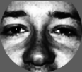
Images were transformed by a FBT up to the 30th Bessel order and 6th root with angular resolution of 3o, thus obtaining to 372 coefficients. These coefficients correspond to a frequency range of up to 30 and 3 cycles/image of angular and radial frequency, respectively, and were selected based on previous tests on a small-size dataset [9]. We tested FBT descriptors of the whole image, or a combination of the upper right region, upper middle region, and the upper left region (Fig. 1). In order to have a better notion of the information retained by the FBT, we used Eq. 1 to reconstruct the image from the FB coefficients. The resulting image has a blurred aspect that reflects the use of only low-frequency radial components. In the rest of this paper, we will refer to the FB transformed images as just images. When using the PFT, the angular sampling was matched and only coefficients related to the same frequency range covered by the FBT were used. Both amplitude and phase information were considered.
| Gallery | Expression | Age |
| Normalized | Inverse FBT | |
 |
3.2 Polar frequency to dissimilarity domain
We built a dissimilarity space defined as the Euclidean distance between all training FBT images . In this space, each object is represented by its dissimilarity to all objects. This approach is based on the assumption that the dissimilarities of similar objects to ”other ones” is about the same [10]. Among other advantages of this representation space, by fixing the number of features to the number of objects, it avoids a well known phenomenon, where recognition performance is degraded as a consequence of small number of training samples as compared to the number of features.
3.3 Classifier
Test images were classified based on a pseudo Fisher linear discriminant (FLD) using a two-class approach. A FLD is obtained by maximizing the (between subjects variation)/(within subjects variation) ratio. Here we used a minimum-square error classifier implementation [11], which is equivalent to the FLD for two-class problems. In these cases, after shifting the data such that it has zero mean, the FLD can be defined as
| (4) |
where is a probe image, is the pooled covariance matrix, and stands for the mean of class . The probe image is classified as corresponding to class-1 if and to class-2 otherwise. However, as the number of objects and dimensions is the same in the dissimilarity space, the sample estimation of the covariance matrix becomes singular and the classifier cannot be built. One solution to the problem is to use a pseudo-inverse and augmented vectors [11]. Thus, Eq. 4 is replaced by
| (5) |
where is the augmented vector to be classified and is the augmented training set. The inverse is the Moore-Penrose Pseudo-inverse which gives the minimum norm solution. The current -classes problem can be reduced and solved by the two-classes solution described above. The training set was split into pairs of subsets, each pair consisting of one subset with images from a single subject and a second subset formed from all the other images. A pseudo-FLD was built for each pair of subsets. A probe image was tested on all discriminant functions, and a “posterior probability” score was generated based on the inverse of the Euclidean distance to each subject.
4 Database, preprocessing, and testing procedures
The main advantages of the FERET database [12] are the large number of individuals and rigid testing protocols that allow precise performance comparisons between different algorithms. We compare our algorithm performance with a ”baseline” PCA-based algorithm [13] and with the results of three successful approaches. The PCA algorithm was based of a set of 700 randomly selected images from the gallery subset. The three first components, that are known to encode basically illumination variations, were excluded prior to image projecting. The other approaches are: Gabor wavelets combined with elastic graph matching [14], localized facial features extraction followed by a Linear Discriminant Analysis (LDA) [15], and a Bayesian generalization of the LDA method [16].
In the FERET protocol, a ”gallery” set of one frontal view image from 1196 subjects is used to train the algorithm and a different dataset is used as probe. We used the probe sets termed ”FB” and ”DupI”. These datasets contain single images from a different number of subjects (1195 and 722, respectively) with differences of facial expression and age, respectively. The ”age” variation subset included several subjects that started or quited wearing glass or grow beards since their ”gallery” pictures were takes. Images were normalized using the eyes ground-truth information or coordinates given by an eyes detector algorithm. This face detection stage was implemented using a cascade of classifiers algorithm for the face detection [17] followed by an Active Appearance Model algorithm (AAM) [18] for the detection of the eyes region. Within this region, we used flow field information [19] to determine the eye center. Approximately 1% of the faces were not localized by the AAM algorithm, in which cases the eyes regions coordinates were set to a fix value derived from the mean of the other faces. The final mean error was 3.7 5.2 pixels. Images were translated, rotated, and scaled so that the eyes were registered at specific pixels (Fig. 1). Next, the images were cropped to 130 x 150 pixels size and a mask was applied to remove most of the hair and background. The unmasked region was histogram equalized and normalized to mean zero and a unit standard deviation.
The system performance was evaluated by verification tests according to the FERET protocol [12]. Given a gallery image and a probe image , the algorithm verifies the claim that both were taken from the same subject. The verification probability is the probability of the algorithm accepting the claim when it is true, and the false-alarm rate is the probability of incorrectly accepting a false claim. The algorithm decision depends on the posterior probability score given to each match, and on a threshold . Thus, a claim is confirmed if and rejected otherwise. A plot of all the combinations of and as a function of is known as a receiver operating characteristic (ROC).
5 Results
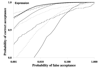
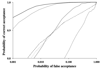
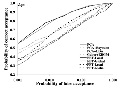
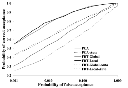
Figure 2 shows the performance of the proposed verification system. The local FBT version performed at the same level of the best previous algorithm (PCA+LDA) on the expression dataset and achieved the best results on the age subset. The global version of the FBT algorithm was inferior at all conditions. Comparisons with the PFT representation indicate that this alternative features are less robust to age and illumination variations. Automation of the eye detection stage reduced the system performance by up to 20%. This reduction is expected, considering the variance property of the FBT to translation [20], and reflect sensitivity to registration errors typical to other algorithms, like the PCA.
We also computed the equal error rate (EER) of the proposed algorithms (Table 1). The EER occurs at a threshold level where the incorrect rejection and false alarm rates are equals (1-). Lower values indicate better performance. The EER results reinforce the conclusions from the ROC functions.
 |
 |
 |
 |
| Semi-Auto | Auto | |||
|---|---|---|---|---|
| Algorithm | Expression | Age | Expression | Age |
| FBT-Global | 1.6 | 7 | 4.5 | 16 |
| FBT-Local | 1.1 | 8 | 7.1 | 16 |
| PFT-Global | 4.1 | 16 | ||
| PFT-Local | 1.4 | 12 | ||
| PCA | 5.9 | 17 | 14 | 23 |
| PCA+Bayesian | 4.9 | 18 | ||
| PCA+LDA | 1.2 | 13 | ||
| Gabor-EBGM | 2.5 | 13 | ||
6 Discussion
Most of the current biologically-inspired algorithms were validated only on very small databases, with the exception of the Gabor-EBGM algorithm that is based on Gabor wavelets transformation and can be viewed as analogous to human spatial filtering at the early stages. Here we presented a novel face verification system based on a local analysis approach and FBT descriptors. The system achieving top ranking on both the age and expression subset. These results are a clear demonstration of the system robustness in handling realistic situations of facial expression and age variations of faces.
The local approach is also superior to the global, a fact that have direct implication for the algorithm robustness for occlusions. In the local approach, the mouth region is ignored, thus its occlusion or variation (ex. due to a new beard) does not affect performance at all. From the computational point of view, the local analysis does not imply much more computation time: the FBT of each region consumes about half the time consumed by the global analysis. Preliminary results (not shown) of the global version with reduced resolution images indicate that computation time can be further with no performance loss, but we still have not tested the effect of image resolution on the local version.
The system have an automatic face detection version, but the trade-off is a certain performance loss. We currently work on the implementation of more precise face and eye detectors algorithms. For example, [21] learned the subspace that represents localization errors within eigenfaces. This method can be easily adopted for the FBT subspace, with the advantage of the option to exclude from the final classification face regions that gives high localization errors.
Currently, we are developing a series of psychophysical experiments with the aim of establishing the relation of the proposed system with human performance. The main questions are: (1) At what location and scale global spatial pooling occurs? (2) Are faces represented in a dissimilarity space? (3) How does filtering of specific polar frequency components affects the face recognition performance of humans and the proposed system?
In conclusion, the proposed system achieved state-of-the-art performance in handling problems of expression and age variations. We expect from future tests to show robustness to illumination variation and partial occlusion and our on-going work are focused on improving the performance of the automatic version.
References
- [1] DeValois, R.L., DeValois, K.K.: Spatial Vision. Oxford Sciences Pub. (1990)
- [2] Perret, D.I. Rolls, E., Caan, W.: Visual neurons responsive to faces in the monkey temporal cortex. Experimental Brain Research 47 (1982) 329–342
- [3] Gallant, J.L. Braun, J., VanEssen, D.: Selectivity for polar, hyperbolic, and cartesian gratings in macaque visual cortex. Science 259 (1993) 100–103
- [4] Wilson, H., Wilkinson, F.: Detection of global structure in glass patterns: implications for form vision. Vision Research 38 (1998) 2933–2947
- [5] Schwartz, E.: Spatial mapping in primate sensory projection: analytic structure and relevance to perception. Biological Cybernetics 25 (1977) 181–194
- [6] Tistarelli, M., Grosso, E.: Active vision-based face recognition issues, applications and techniques. In: NatoAsi Advanced Study on Face Recognition. Volume F-163. Springer-Berlin (1998) 262–286 Ed.: Wechsler, H. et al.
- [7] Bowman, F.: Introduction to Bessel functions. Dover Pub., New York (1958)
- [8] Fox, P., Cheng, J., Lu, J.: Theory and experiment of Fourier-Bessel field calculation and tuning of a pulsed wave annular array. Journal of the Acoustical Society of America 113 (2003) 2412–2423
- [9] Zana, Y., Cesar-Jr, R.M.: Face recognition based on polar frequency features. ACM Transactions on Applied Perception 2 (2005) To appear.
- [10] Duin, R., DeRidder, D., Tax, D.: Experiments with a featureless approach to pattern recognition. Pattern Recognition Letters 18 (1997) 1159–1166
- [11] Scurichina, M., Duin, R.: Stabilizing classifiers for very small sample sizes. In: Proceedings of the 13th International Conference on Pattern Recognition. Volume 2, Track B. (1996) 891–896
- [12] Phillips, P., Wechsler, H., Huang, J., Rauss, P.: The FERET database and evaluation procedure for face recognition algorithms. Image and Vision Computing Journal 16 (1998) 295–306
- [13] Turk, M., Pentland, A.: Eigenfaces for recognition. Journal of Cognitive Neuroscience 3 (1991) 71–86
- [14] Wiskott, L., Fellous, J., Kruger, N., VonDerMalsburg, C.: Face recognition by elastic bunch graph matching. IEEE Transactions on Pattern Analysis and Machine Intelligence 19 (1997) 775–779
- [15] Etemad, K., Chellappa, R.: Discriminant analysis for recognition of human face images. Journal of the Optical Society of America A-Optics Image Science and Vision 14 (1997) 1724–1733
- [16] Moghaddam, B., Jebara, T., Pentland, A.: Bayesian face recognition. Pattern Recognition 33 (2000) 1771–1782
- [17] Viola, P., Jones, M.: Rapid object detection using a boosted cascade of simple features. In: IEEE Conference on Computer Vision and Pattern Recognition (CVPR). (2001) 511–518
- [18] Cootes, T., Edwards, G., Taylor, C.: Active appearance models. IEEE Transactions on Pattern Analysis and Machine Intelligence 23 (2001) 681–685
- [19] Kothari, R., Mitchell, J.: Detection of eye locations in unconstrained visual images. In: IEEE International Conference on Image Processing. (1996) 519–522
- [20] Cabrera, J., Falcón, A., Hernández, F., Méndez, J.: A systematic method for exploring contour segment descriptions. Cybernetics and Systems 23 (1992) 241–270
- [21] Martínez, A.: Recognizing imprecisely localized, partially occluded, and expression variant faces from a single sample per class. IEEE Transactions on Pattern Analysis and Machine Intelligence 24 (2002) 748–762