On the Capacity of Doubly Correlated MIMO Channels

Abstract

In this paper, we analyze the capacity of multiple-input multiple-output (MIMO) Rayleigh-fading channels in the presence of spatial fading correlation at both the transmitter and the receiver, assuming that the channel is unknown at the transmitter and perfectly known at the receiver. We first derive the determinant representation for the exact characteristic function of the capacity, which is then used to determine the trace representations for the mean, variance, skewness, kurtosis, and other higher-order statistics (HOS). These results allow us to exactly evaluate two relevant information-theoretic capacity measures—ergodic capacity and outage capacity—and the HOS of the capacity for such a MIMO channel. The analytical framework presented in the paper is valid for arbitrary numbers of antennas and generalizes the previously known results for independent and identically distributed or one-sided correlated MIMO channels to the case when fading correlation exists on both sides. We verify our analytical results by comparing them with Monte Carlo simulations for a correlation model based on realistic channel measurements as well as a classical exponential correlation model.

I Introduction

Multiple-input multiple-output (MIMO) communication systems using multiple transmit and receive antennas promise high spectral efficiency and link reliability for wireless communications [1, 2, 3]. Although the linear growth of capacity with the number of antennas indicates the potential of MIMO systems, the true benefits of the use of multiple antennas may be limited by spatial fading correlation due to closely-spaced antenna configurations and poor scattering environments in realistic wireless channels [4, 5].

Since the pioneering work of [1, 2, 3] in the area of multiple-antenna communications predicted remarkable spectral efficiency of MIMO wireless systems in independent and identically distributed (i.i.d.) Rayleigh fading, much subsequent work has concentrated on characterizing MIMO capacity under correlated fading [4, 5, 6, 7, 8, 9, 10, 11, 12, 13, 14]. However, the exact analytical results for the capacity such as ergodic (or mean) capacity, capacity variance, and outage capacity (i.e., capacity versus outage probability) have been known for only a few special cases, largely due to mathematical intractability (see, e.g., [3, 6, 16] for i.i.d. flat Rayleigh fading and [7, 8, 9] for a one-sided correlated MIMO channel). For a more general case of correlated fading at both the transmitter and the receiver, which we will refer to as doubly correlated MIMO channels in the paper, some limited results are available: the capacity distribution for a small number of antennas (i.e., $\min\left\{{n_{\mathrm{T}}},{n_{\mathrm{R}}}\right\}\leq 3$ where ${n_{\mathrm{T}}}$ and ${n_{\mathrm{R}}}$ are the numbers of transmit and receive antennas, respectively) [10], upper and lower bounds on the ergodic capacity [6, 12], capacity statistics for the case with a large number of antennas [13], and the asymptotic mean and variance of the capacity in the limit as the number of antennas tends to infinity [5, 14]. The temporal behavior of the capacity was analyzed in [11] in terms of level crossing rates and average fade durations.

In this paper, we focus on deriving the exact analytical expressions for capacity statistics of doubly correlated MIMO Rayleigh-fading channels using the methodology developed in [6] and [7], assuming perfect channel knowledge at the receiver and no knowledge at the transmitter with the average input-power constraint. The principal contributions of this paper are as follows.

• We derive a determinant representation for the characteristic function (CF) of MIMO capacity, which generalizes the previous results for i.i.d. and one-sided correlated channels [7, 8, 9] to the doubly correlated case.

• We derive trace representations for the mean, variance, and higher-order statistics (HOS) (e.g., cumulants, skewness, and kurtosis) of the capacity using the determinant representation of the CF and the relationship between polymatrices and dimatrices.

• We characterize the effect of fading correlation on the capacity statistics at high signal-to-noise ratio (SNR). We show that at high SNR, the variance, skewness, kurtosis, and other HOS of the capacity depend only on correlation at the side with the larger number of antennas. Moreover, when ${n_{\mathrm{T}}}={n_{\mathrm{R}}}$, these statistics are not affected by fading correlation at any side.

To verify our analytical results, we also compare them with Monte Carlo simulations for doubly correlated MIMO channels using a correlation model based on physical measurements [17, 18] as well as a classical exponential correlation model. It should be noted that alternative derivation of the moment generating function (MGF) of the capacity for doubly correlated MIMO channels can also be found in [19]. In this study, the MGF was obtained indirectly from the case of a square channel matrix (${n_{\mathrm{T}}}={n_{\mathrm{R}}}$) using the limiting approach of [20] and then, the first moment (ergodic capacity) was deduced from it in terms of a sum of $\min\left\{{n_{\mathrm{T}}},{n_{\mathrm{R}}}\right\}$ determinants.

The remainder of the paper is organized as follows. A brief overview of the distributions of complex random matrices required for our analysis, channel model, and associated channel capacity are presented in Section II. The CF of the capacity is derived and the capacity statistics are analyzed for doubly correlated MIMO channels in Section III. The effect of fading correlation on the capacity statistics is investigated at high SNR in Section IV. In Section V, some numerical and simulation results are provided to illustrate our analytical results. Finally, Section VI concludes the paper.

We shall use the following notation throughout the paper. $\mathbb{N}$ and $\mathbb{C}$ denote the natural numbers and the field of complex numbers, respectively. The superscript ${\dagger}$ denotes the transpose conjugate. ${\mathbf{I}}_{n}$ and $\operatorname{\mathrm{tr}}\left({\mathbf{A}}\right)$ represent the $n\times n$ identity matrix and the trace operator of a square matrix ${\mathbf{A}}$, respectively. By ${\mathbf{A}}>0$, we denote that ${\mathbf{A}}$ is positive definite. For a matrix ${\mathbf{A}}\left(t\right)=\left[a_{i,j}\left(t\right)\right]$ where $a_{i,j}\left(t\right)$ are differentiable functions of $t$, the $n$th derivative of ${\mathbf{A}}\left(t\right)$ with respect to $t$ is denoted by ${\mathbf{A}}^{\left(n\right)}\left(t\right)=\left[d^{n}a_{i,j}\left(t\right)/dt^{n}\right]$.

II Preliminaries: Definitions and Models

In this section, we give a brief overview of the distribution theory of complex random matrices (that serves as a central mathematical tool to analyze MIMO communication systems), channel model, and associated channel capacity.

II-A Distributions of Complex Random Matrices

Let us denote a complex Gaussian matrix ${\mathbf{X}}\in\mathbb{C}^{m\times n}$ with the probability density function (PDF) [6, eq. (1)]

$$p_{{{\mathbf{X}}}}\left({{\mathbf{X}}}\right)=\pi^{-mn}\det\left({\mathbf{\Sigma}}\right)^{-n}\det\left({\mathbf{\Psi}}\right)^{-m}e^{-\operatorname{\mathrm{tr}}\left\{{\mathbf{\Sigma}}^{-1}\left({\mathbf{X}}-{\mathbf{M}}\right){\mathbf{\Psi}}^{-1}\left({\mathbf{X}}-{\mathbf{M}}\right)^{\dagger}\right\}}$$ (1)

by ${\mathbf{X}}\sim\tilde{\mathcal{N}}_{{m},{n}}\left({{\mathbf{M}}},{{\mathbf{\Sigma}}},{{\mathbf{\Psi}}}\right)$ where ${\mathbf{\Sigma}}\in\mathbb{C}^{m\times m}>0$ and ${\mathbf{\Psi}}\in\mathbb{C}^{n\times n}>0$ are Hermitian. If ${\mathbf{X}}\sim\tilde{\mathcal{N}}_{{m},{n}}\left({{\mathbf{0}}},{{\mathbf{\Sigma}}},{{\mathbf{I}}_{n}}\right)$, $m\leq n$, and ${\mathbf{Y}}={\mathbf{XX}}^{\dagger}$, then ${\mathbf{Y}}$ has a complex (central) Wishart density $\tilde{\mathcal{W}}_{m}\left({n},{{\mathbf{\Sigma}}}\right)$ given by [6, eq. (3)].

Definition 1 (Quadratic Form in the Complex Gaussian Matrix [6])

Let

$${\mathbf{X}}\sim\tilde{\mathcal{N}}_{{m},{n}}\left({{\mathbf{0}}},{{\mathbf{\Sigma}}},{{\mathbf{\Psi}}}\right),\quad m\leq n.$$

A positive-definite quadratic form ${\mathbf{Y}}$ in ${\mathbf{X}}$ associated with a Hermitian matrix ${\mathbf{A}}\in\mathbb{C}^{n\times n}>0$, denoted by ${\mathbf{Y}}\sim\tilde{Q}_{{m},{n}}\left({{\mathbf{A}}},{{\mathbf{\Sigma}}},{{\mathbf{\Psi}}}\right)$, is then defined as ${\mathbf{Y}}={\mathbf{XAX}}^{\dagger}$.

The PDF of ${\mathbf{Y}}\sim\tilde{Q}_{{m},{n}}\left({{\mathbf{A}}},{{\mathbf{\Sigma}}},{{\mathbf{\Psi}}}\right)$ is given by [21, eq. (57)] and can be expressed in an equivalent form

$$p_{{{\mathbf{Y}}}}\left({{\mathbf{Y}}}\right) =\frac{1}{\tilde{\Gamma}_{m}\left(n\right)}\det\left({\mathbf{\Sigma}}\right)^{-n}\det\left({\mathbf{A}}{\mathbf{\Psi}}\right)^{-m}\det\left({\mathbf{Y}}\right)^{n-m}{}_{0}\tilde{F}_{0}^{\left(n\right)}\left(-{\mathbf{\Sigma}}^{-1}{\mathbf{Y}},{\mathbf{\Psi}}^{-1}{\mathbf{A}}^{-1}\right),~{}{\mathbf{Y}}>0$$ (2)

where $\tilde{\Gamma}_{m}\left(\alpha\right)=\pi^{m\left(m-1\right)/2}\prod\nolimits_{i=0}^{m-1}{\Gamma\left({\alpha-i}\right)}$, $\mathrm{Re}\left(\alpha\right)>m-1$, is the complex multivariate gamma function, $\Gamma\left(\cdot\right)$ is the gamma function, and ${}_{p}\tilde{F}_{q}^{\left(n\right)}\left(\cdot\right)$ is the hypergeometric function of two Hermitian matrices, defined by [21, eq. (51)]. Note that the density (2) is a counterpart of the real case in [22, eq. (7.2.5)] and if ${\mathbf{A}}{\mathbf{\Psi}}={\mathbf{I}}_{n}$, it reduces to the complex Wishart density $\tilde{\mathcal{W}}_{m}\left({n},{{\mathbf{\Sigma}}}\right)$.

II-B Channel Model and Capacity Random Variable

We consider a point-to-point frequency-flat fading MIMO link with ${n_{\mathrm{T}}}$ transmit and ${n_{\mathrm{R}}}$ receive antennas. Let ${\mathbf{x}}\in\mathbb{C}^{{n_{\mathrm{T}}}}$ be a transmitted signal vector with input covariance ${\mathbf{Q}}=\operatorname{\mathbb{E}}\left\{{{\mathbf{xx}}^{\dagger}}\right\}$ satisfying the power constraint $\operatorname{\mathrm{tr}}\left({\mathbf{Q}}\right)\leq\mathcal{P}$, then the received signal is given by

$${\mathbf{y}}={\mathbf{H}}{\mathbf{x}}+{\mathbf{n}}$$ (3)

where ${\mathbf{H}}\in\mathbb{C}^{{n_{\mathrm{R}}}\times{n_{\mathrm{T}}}}$ is the random channel matrix whose $\left(i,j\right)$th entries $H_{ij}$, $i=1,2,\ldots,{n_{\mathrm{R}}}$, $j=1,2,\ldots,{n_{\mathrm{T}}}$, are complex propagation coefficients between the $j$th transmit antenna and the $i$th receive antenna with $\operatorname{\mathbb{E}}\left\{{|H_{ij}|^{2}}\right\}=1$, and ${\mathbf{n}}$ is the complex ${n_{\mathrm{R}}}$-dimensional zero-mean additive white Gaussian noise (AWGN) vector with the covariance matrix $\sigma_{n}^{2}{\mathbf{I}}_{{n_{\mathrm{R}}}}$. For doubly correlated MIMO channels, the channel matrix ${\mathbf{H}}$ can be written as [4, 5]

$${\mathbf{H}}={\mathbf{\Psi}}_{\mathrm{R}}^{1/2}{\mathbf{H}}_{\text{uc}}{\mathbf{\Psi}}_{\mathrm{T}}^{1/2}$$ (4)

where ${\mathbf{H}}_{\text{uc}}\sim\tilde{\mathcal{N}}_{{{n_{\mathrm{R}}}},{{n_{\mathrm{T}}}}}\left({{\mathbf{0}}},{{\mathbf{I}}_{n_{\mathrm{R}}}},{{\mathbf{I}}_{n_{\mathrm{T}}}}\right)$, and ${\mathbf{\Psi}}_{\mathrm{T}}\in\mathbb{C}^{{n_{\mathrm{T}}}\times{n_{\mathrm{T}}}}>0$ and ${\mathbf{\Psi}}_{\mathrm{R}}\in\mathbb{C}^{{n_{\mathrm{R}}}\times{n_{\mathrm{R}}}}>0$ are the transmit and receive correlation matrices, respectively. Note that ${\mathbf{H}}\sim\tilde{\mathcal{N}}_{{{n_{\mathrm{R}}}},{{n_{\mathrm{T}}}}}\left({{\mathbf{0}}},{{\mathbf{\Psi}}_{\mathrm{R}}},{{\mathbf{\Psi}}_{\mathrm{T}}}\right)$ and it has been used in various attempts for studying correlated MIMO channels [4, 5, 6, 7, 8, 9, 10, 11, 12, 13, 14]. Recently, this model has also been validated through physical measurements [17].

In what follows, we refer to ${n_{\mathrm{S}}}=\min\left\{{n_{\mathrm{T}}},{n_{\mathrm{R}}}\right\}$ and ${n_{\mathrm{L}}}=\max\left\{{n_{\mathrm{T}}},{n_{\mathrm{R}}}\right\}$ and define the random matrix ${\mathbf{\Theta}}\in\mathbb{C}^{{n_{\mathrm{S}}}\times{n_{\mathrm{S}}}}>0$ as

$${\mathbf{\Theta}}\triangleq\begin{cases}{\mathbf{HH}}^{\dagger},&\text{if }{n_{\mathrm{R}}}\leq{n_{\mathrm{T}}}\\[-5.69054pt] {\mathbf{H}}^{\dagger}{\mathbf{H}},&\text{otherwise}.\end{cases}\vspace*{5pt}$$

Also, let us denote, for convenience,

$$\left({\mathbf{\Psi}}_{\mathrm{S}},{\mathbf{\Psi}}_{\mathrm{L}}\right)=\begin{cases}\left({\mathbf{\Psi}}_{\mathrm{R}},{\mathbf{\Psi}}_{\mathrm{T}}\right),&\text{if }{n_{\mathrm{R}}}\leq{n_{\mathrm{T}}}\\[-5.69054pt] \left({\mathbf{\Psi}}_{\mathrm{T}},{\mathbf{\Psi}}_{\mathrm{R}}\right),&\text{otherwise}\end{cases}$$

and let $0<\lambda_{\mathrm{S},{1}}<\lambda_{\mathrm{S},{2}}<\cdots<\lambda_{\mathrm{S},{{n_{\mathrm{S}}}}}$ and $0<\lambda_{\mathrm{L},{1}}<\lambda_{\mathrm{L},{2}}<\cdots<\lambda_{\mathrm{L},{{n_{\mathrm{L}}}}}$ be distinct ordered eigenvalues of ${\mathbf{\Psi}}_{\mathrm{S}}$ and ${\mathbf{\Psi}}_{\mathrm{L}}$, respectively. Then, ${\mathbf{\Theta}}\sim\tilde{Q}_{{{n_{\mathrm{S}}}},{{n_{\mathrm{L}}}}}\left({{\mathbf{I}}_{n_{\mathrm{L}}}},{{\mathbf{\Psi}}_{\mathrm{S}}},{{\mathbf{\Psi}}_{\mathrm{L}}}\right)$ for the doubly correlated MIMO channel.

In general, when the receiver has perfect channel knowledge, the input distribution that maximizes the mutual information between ${\mathbf{x}}$ and ${\mathbf{y}}$ is circularly symmetric complex Gaussian for any given input covariance ${\mathbf{Q}}$. When the transmitter has no channel knowledge, power among transmit antennas cannot be allocated in accordance with the realization of ${\mathbf{H}}$ to maximize the mutual information, and hence equal power allocation to each of transmit antennas is the most reasonable strategy, i.e., choosing ${\mathbf{Q}}=\left(\mathcal{P}/{n_{\mathrm{T}}}\right){\mathbf{I}}_{n_{\mathrm{T}}}$. This yields the capacity in nats/s/Hz as [2, 3]

$$C=\ln\det\left({\mathbf{I}}_{n_{\mathrm{S}}}+\left(\eta/{n_{\mathrm{T}}}\right){\mathbf{\Theta}}\right)$$ (5)

where $\eta=\mathcal{P}/\sigma_{n}^{2}$ is the average SNR at each receive antenna. Since the channel matrix ${\mathbf{H}}$ is random, the associated channel capacity $C$ is also a random variable whose statistics are determined by the statistical properties of the eigenvalues of ${\mathbf{\Theta}}\sim\tilde{Q}_{{{n_{\mathrm{S}}}},{{n_{\mathrm{L}}}}}\left({{\mathbf{I}}_{n_{\mathrm{L}}}},{{\mathbf{\Psi}}_{\mathrm{S}}},{{\mathbf{\Psi}}_{\mathrm{L}}}\right)$.

III Capacity Statistics

In this section, we will investigate the statistical properties of the capacity random variable $C$ in (5) for doubly correlated MIMO channels. We begin by deriving the CF of $C$, from which all other functions, such as the PDF, cumulative distribution function (CDF), and cumulant generating function (CGF), and statistical moments of $C$ can be obtained.

III-A Characteristic Function

Theorem 1

Let ${\mathbf{H}}\sim\tilde{\mathcal{N}}_{{{n_{\mathrm{R}}}},{{n_{\mathrm{T}}}}}\left({{\mathbf{0}}},{{\mathbf{\Psi}}_{\mathrm{R}}},{{\mathbf{\Psi}}_{\mathrm{T}}}\right)$, i.e., ${\mathbf{\Theta}}\sim\tilde{Q}_{{{n_{\mathrm{S}}}},{{n_{\mathrm{L}}}}}\left({{\mathbf{I}}_{n_{\mathrm{L}}}},{{\mathbf{\Psi}}_{\mathrm{S}}},{{\mathbf{\Psi}}_{\mathrm{L}}}\right)$. Then, the CF of the capacity $C$ in nats/s/Hz is

$$\Phi_{C}\left({\jmath\omega}\right) \triangleq\operatorname{\mathbb{E}}\left\{{e^{\jmath\omega C}}\right\}$$

$$=K_{\mathrm{cor}}^{-1}\,\Upsilon_{n_{\mathrm{S}}}\left(\jmath\omega\right)\,\det{\mathbf{\Lambda}}\left(\jmath\omega\right)$$ (6)

where $\jmath=\sqrt{-1}$ and

$$K_{\mathrm{cor}}=\left(\frac{\eta}{{n_{\mathrm{T}}}}\right)^{{n_{\mathrm{S}}}\left({n_{\mathrm{S}}}-1\right)/2}\prod_{1\leq i<j\leq{n_{\mathrm{S}}}}\left(\lambda_{\mathrm{S},{j}}-\lambda_{\mathrm{S},{i}}\right)\prod_{1\leq i<j\leq{n_{\mathrm{L}}}}\left(\lambda_{\mathrm{L},{j}}-\lambda_{\mathrm{L},{i}}\right)$$ (7)

$$\Upsilon_{n_{\mathrm{S}}}\left(\jmath\omega\right)=\prod_{\ell=1}^{{n_{\mathrm{S}}}-1}\left(\jmath\omega+\ell\right)^{-\ell}$$ (8)

and ${\mathbf{\Lambda}}\left(\jmath\omega\right)$ is the ${n_{\mathrm{L}}}\times{n_{\mathrm{L}}}$ matrix whose $\left(i,j\right)$th entry is given in Table I.

Proof:

See Appendix B. ∎

Note that Theorem 1 requires correlation matrices ${\mathbf{\Psi}}_{\mathrm{T}}$ and ${\mathbf{\Psi}}_{\mathrm{R}}$ to have distinct eigenvalues. The case when the correlation matrices have non-distinct eigenvalues (some of $\lambda_{\mathrm{S},{i}}$’s or $\lambda_{\mathrm{L},{i}}$’s are equal), we can obtain the CF as a limiting case of (1) [7, 23]. In particular, when ${\mathbf{\Psi}}_{\mathrm{T}}={\mathbf{I}}_{{n_{\mathrm{T}}}}$ and ${\mathbf{\Psi}}_{\mathrm{R}}={\mathbf{I}}_{{n_{\mathrm{R}}}}$ (i.i.d. case), $\Phi_{C}\left({\jmath\omega}\right)$ is given by [7, eq. (25)]

$$\Phi_{C}\left({\jmath\omega}\right)=K_{\mathrm{iid}}^{-1}\,\det{\mathbf{\Omega}}\left(\jmath\omega\right)$$ (9)

where $K_{\mathrm{iid}}=\prod_{\ell=1}^{n_{\mathrm{S}}}\left({n_{\mathrm{L}}}-\ell\right)!\left(\ell-1\right)!$ and ${\mathbf{\Omega}}\left(\jmath\omega\right)$ is the ${n_{\mathrm{S}}}\times{n_{\mathrm{S}}}$ Hankel matrix whose $\left(i,j\right)$th entry is given in Table I. Theorem 1 generalizes the previous results for i.i.d. and one-sided correlated channels (which are special cases of non-distinct eigenvalues) [7, 8, 9] to the doubly correlated MIMO channel given by (4). Using the analytical formulas for the CF in (1) and (9), the PDF and CDF of $C$ can be expressed in forms of the inverse Fourier transform of $\Phi_{C}\left({\jmath\omega}\right)$, which can be efficiently calculated by using the fast Fourier transform (FFT) method [7, 24].

III-B Mean, Variance, and Higher-Order Statistics

From the CF of $C$ in (1) and (9) involving the determinants, we derive the exact closed-form expressions for the mean, variance, and other HOS such as cumulants, skewness, and (excess) kurtosis of the capacity. To do this, we first introduce the logarithmic derivative of a determinant.

III-B1 Logarithmic Derivatives of a Determinant

Let ${\mathbf{R}}\left(t\right)$ be a matrix depending on a parameter $t$. If each entry of ${\mathbf{R}}\left(t\right)$ is differentiable with respect to $t$, then so is $\det{\mathbf{R}}\left(t\right)$ because the determinant is a polynomial in the entries of ${\mathbf{R}}\left(t\right)$. If ${\mathbf{R}}\left(t\right)$ is invertible, the first-order logarithmic derivative of $\det{\mathbf{R}}\left(t\right)$ is given by [25]

$$\frac{d\ln\det{\mathbf{R}}\left(t\right)}{dt}=\operatorname{\mathrm{tr}}\left\{{\mathbf{R}}^{-1}\left(t\right){\mathbf{R}}^{\left(1\right)}\left(t\right)\right\}.$$ (10)

We now generalize (10) to the arbitrary order of differentiation.

Definition 2 (Polymatrix and Dimatrix)

Let ${\mathbf{R}}\left(t\right)$ be an invertible matrix whose elements are differentiable with respect to $t$. Then, the $n$th polymatrix of ${\mathbf{R}}\left(t\right)$ with respect to $t$ is defined as

$${\mathbf{R}}_{\left[n\right]}\left(t\right)\triangleq{\mathbf{R}}^{-1}\left(t\right){\mathbf{R}}^{\left(n\right)}\left(t\right).$$ (11)

In particular, we call ${\mathbf{R}}_{\left[1\right]}\left(t\right)$ the dimatrix of ${\mathbf{R}}\left(t\right)$.

Lemma 1

The polymatrices and the derivatives of the dimatrix of ${\mathbf{R}}\left(t\right)$ have the following relationship

$${\mathbf{R}}_{\left[n\right]}\left(t\right)=\sum_{\ell=1}^{n}\binom{n-1}{\ell-1}{\mathbf{R}}_{\left[n-\ell\right]}\left(t\right){\mathbf{R}}_{\left[1\right]}^{\left(\ell-1\right)}\left(t\right)$$ (12)

and the $\ell$th logarithmic derivative of $\det{\mathbf{R}}\left(t\right)$ is the trace of the $\left(\ell-1\right)$th derivative of the dimatrix ${\mathbf{R}}_{\left[1\right]}\left(t\right)$, i.e.,

$$\frac{d^{\ell}\ln\det{\mathbf{R}}\left(t\right)}{dt^{\ell}}=\operatorname{\mathrm{tr}}\left\{{\mathbf{R}}_{\left[1\right]}^{\left(\ell-1\right)}\left(t\right)\right\}.$$ (13)

Proof:

By definition, we have

$${\mathbf{R}}_{\left[n\right]}\left(t\right) ={\mathbf{R}}^{-1}\left(t\right)\frac{d^{n-1}{\mathbf{R}}^{\left(1\right)}\left(t\right)}{dt^{n-1}}$$

$$\stackrel{{\scriptstyle\left(a\right)}}{{=}}{\mathbf{R}}^{-1}\left(t\right)\sum_{\ell=1}^{n}\binom{n-1}{\ell-1}\frac{d^{n-\ell}{\mathbf{R}}\left(t\right)}{dt^{n-\ell}}\frac{d^{\ell-1}{\mathbf{R}}_{\left[1\right]}\left(t\right)}{dt^{\ell-1}}$$

$$\stackrel{{\scriptstyle\left(b\right)}}{{=}}\sum_{\ell=1}^{n}\binom{n-1}{\ell-1}{\mathbf{R}}_{\left[n-\ell\right]}\left(t\right){\mathbf{R}}_{\left[1\right]}^{\left(\ell-1\right)}\left(t\right)$$

where (a) follows from the Leibniz’s identity [26, p. 21] and (b) follows from (11). Also, (13) follows immediately from (10), (11), and by interchanging the order of differentiation and trace operators. ∎

This lemma says that the $\ell$th logarithmic derivative of the determinant of a matrix can be determined by its first $\ell$ polymatrices. For example, the second, third, and fourth order logarithmic derivatives of $\det{\mathbf{R}}\left(t\right)$ are given by

$$\frac{d^{2}\ln\det{\mathbf{R}}\left(t\right)}{dt^{2}} =\operatorname{\mathrm{tr}}\left\{{\mathbf{R}}_{\left[2\right]}\left(t\right)-{\mathbf{R}}_{\left[1\right]}^{2}\left(t\right)\right\}$$ (14)

$$\frac{d^{3}\ln\det{\mathbf{R}}\left(t\right)}{dt^{3}} =\operatorname{\mathrm{tr}}\left\{2{\mathbf{R}}_{\left[1\right]}^{3}\left(t\right)-3{\mathbf{R}}_{\left[1\right]}\left(t\right){\mathbf{R}}_{\left[2\right]}\left(t\right)+{\mathbf{R}}_{\left[3\right]}\left(t\right)\right\}$$ (15)

$$\frac{d^{4}\ln\det{\mathbf{R}}\left(t\right)}{dt^{4}} =\operatorname{\mathrm{tr}}\left\{-6{\mathbf{R}}_{\left[1\right]}^{4}\left(t\right)+12{\mathbf{R}}_{\left[1\right]}^{2}\left(t\right){\mathbf{R}}_{\left[2\right]}\left(t\right)\right.$$

$$\qquad\quad\left.-3{\mathbf{R}}_{\left[2\right]}^{2}\left(t\right)-4{\mathbf{R}}_{\left[1\right]}\left(t\right){\mathbf{R}}_{\left[3\right]}\left(t\right)+{\mathbf{R}}_{\left[4\right]}\left(t\right)\right\}.$$ (16)

Using the explicit determinantal CF’s in Section III-A and Lemma 1, we now derive statistical moments of $C$, which requires determining the polymatrices

$${\mathbf{\Omega}}_{\left[n\right]}\left(\nu\right)={\mathbf{\Omega}}^{-1}\left(\nu\right){\mathbf{\Omega}}^{\left(n\right)}\left(\nu\right),\quad{\mathbf{\Omega}}_{\left[0\right]}\left(\nu\right)={\mathbf{I}}_{n_{\mathrm{S}}}$$ (17)

$${\mathbf{\Lambda}}_{\left[n\right]}\left(\nu\right)={\mathbf{\Lambda}}^{-1}\left(\nu\right){\mathbf{\Lambda}}^{\left(n\right)}\left(\nu\right),\quad{\mathbf{\Lambda}}_{\left[0\right]}\left(\nu\right)={\mathbf{I}}_{n_{\mathrm{L}}}$$ (18)

for i.i.d. and doubly correlated MIMO channels, respectively, where the $(i,j)$th entries of ${\mathbf{\Omega}}^{\left(n\right)}\left(\nu\right)$ and ${\mathbf{\Lambda}}^{\left(n\right)}\left(\nu\right)$ for $n\in\mathbb{N}$ are given in Table I.

III-B2 Cumulants

The $n$th cumulant of $C$ is by definition expressed as

$$\kappa_{n}\triangleq\left.\frac{d^{n}}{d\nu^{n}}\mathcal{K}_{C}\left({\nu}\right)\right|_{\nu=0}$$ (19)

where $\mathcal{K}_{C}\left({\nu}\right)\triangleq\ln\Phi_{C}\left({\nu}\right)$ is the CGF of $C$. Note that the first and second cumulants are the mean and variance of the capacity, respectively.

Theorem 2

Let ${\mathbf{H}}\sim\tilde{\mathcal{N}}_{{{n_{\mathrm{R}}}},{{n_{\mathrm{T}}}}}\left({{\mathbf{0}}},{{\mathbf{I}}_{n_{\mathrm{R}}}},{{\mathbf{I}}_{n_{\mathrm{T}}}}\right)$, i.e., ${\mathbf{\Theta}}\sim\tilde{\mathcal{W}}_{{n_{\mathrm{S}}}}\left({{n_{\mathrm{L}}}},{{\mathbf{I}}_{n_{\mathrm{S}}}}\right)$ (${n_{\mathrm{R}}}\times{n_{\mathrm{T}}}$ i.i.d. MIMO channel). Then, the $n$th cumulant of the capacity $C$ in nats/s/Hz is

$$\kappa_{n}=\operatorname{\mathrm{tr}}\left\{{\mathbf{\Omega}}_{\left[1\right]}^{\left(n-1\right)}\left(0\right)\right\}.\vspace*{5pt}$$ (20)

Proof:

It follows immediately from (9), (19), and Lemma 1. ∎

Theorem 3

Let ${\mathbf{H}}\sim\tilde{\mathcal{N}}_{{{n_{\mathrm{R}}}},{{n_{\mathrm{T}}}}}\left({{\mathbf{0}}},{{\mathbf{\Psi}}_{\mathrm{R}}},{{\mathbf{\Psi}}_{\mathrm{T}}}\right)$, i.e., ${\mathbf{\Theta}}\sim\tilde{Q}_{{{n_{\mathrm{S}}}},{{n_{\mathrm{L}}}}}\left({{\mathbf{I}}_{n_{\mathrm{L}}}},{{\mathbf{\Psi}}_{\mathrm{S}}},{{\mathbf{\Psi}}_{\mathrm{L}}}\right)$ (${n_{\mathrm{R}}}\times{n_{\mathrm{T}}}$ doubly correlated MIMO channel). Then, the $n$th cumulant of the capacity $C$ in nats/s/Hz is

$$\kappa_{n}=\operatorname{\mathrm{tr}}\left\{{\mathbf{\Lambda}}_{\left[1\right]}^{\left(n-1\right)}\left(0\right)\right\}+\left(-1\right)^{n}\left(n-1\right)!\sum_{\ell=1}^{{n_{\mathrm{S}}}-1}\ell^{-n+1}.\vspace*{5pt}$$ (21)

Proof:

It follows immediately from Theorem 1, (19), and Lemma 1. ∎

Using the relationship (12), the matrices ${\mathbf{\Omega}}_{\left[1\right]}^{\left(n-1\right)}\left(\nu\right)$ and ${\mathbf{\Lambda}}_{\left[1\right]}^{\left(n-1\right)}\left(\nu\right)$ in Theorems 2 and 3 can be determined by the polymatrices in (17) and (18), respectively.

III-B3 Raw and Central Moments

The $n$th raw and central moments (i.e., moments about the origin and the mean, respectively) of $C$ can be obtained from the general relationships between moments and cumulants [27]:

$$m_{n}\triangleq\operatorname{\mathbb{E}}\left\{{C^{n}}\right\}=\sum_{\ell=1}^{n}\binom{n-1}{\ell-1}m_{n-\ell}\,\kappa_{\ell}$$ (22)

$$\mu_{n}\triangleq\operatorname{\mathbb{E}}\left\{{\left(C-m_{1}\right)^{n}}\right\}=\sum_{\ell=0}^{n}\binom{n}{\ell}m_{n-\ell}\left(-m_{1}\right)^{\ell}$$ (23)

where $m_{n}$ and $\mu_{n}$ are the $n$th raw and central moments of $C$, respectively. In particular, the ergodic capacity is given by $m_{1}=\operatorname{\mathbb{E}}\left\{{C}\right\}$.

III-B4 Skewness and Kurtosis

The skewness characterizes the degree of asymmetry of a distribution around its mean and the kurtosis measures the peakedness or flatness of a distribution relative to a Gaussian distribution. The skewness and (excess) kurtosis of $C$, denoted by $\beta_{1}$ and $\beta_{2}$, respectively, can be obtained from the cumulants in Theorems 2 and 3 for i.i.d. and doubly correlated cases as

$$\beta_{1}\triangleq\frac{\mu_{3}}{\mu_{2}^{3/2}}=\frac{\kappa_{3}}{\kappa_{2}^{3/2}}$$ (24)

$$\beta_{2}\triangleq\frac{\mu_{4}}{\mu_{2}^{2}}-3=\frac{\kappa_{4}}{\kappa_{2}^{2}}.$$ (25)

Using (14)–(III-B1), (20), (21), (24), and (25), the trace representations for the mean, variance, skewness, and kurtosis of the capacity are tabulated in Tables II and III for i.i.d. and doubly correlated MIMO channels, respectively. Since the skewness and kurtosis of a Gaussian distribution are equal to zero, nonzero values of these quantities indicate the degree of deviation from the Gaussian distribution.

IV Effect of Correlation at High SNR

The effect of fading correlation on the behavior of capacity is not immediately apparent from the exact analytical expressions such as the CF in (1) and the moments in Table III. Therefore, we resort to the asymptotic analysis to investigate such an effect in the following. In particular, we consider a high-SNR regime since the benefits of the use of multiple antennas are more pronounced at high SNR. In this case, the capacity (5) can be written as

$$C={n_{\mathrm{S}}}\ln\left(\eta/{n_{\mathrm{T}}}\right)+\ln\det\left({\mathbf{\Theta}}\right)+O\left(1/\eta\right),$$ (26)

which reveals that at high SNR, the capacity is characterized by the logarithmic generalized variance $\ln\det\left({\mathbf{\Theta}}\right)$ of ${\mathbf{\Theta}}\sim\tilde{Q}_{{{n_{\mathrm{S}}}},{{n_{\mathrm{L}}}}}\left({{\mathbf{I}}_{n_{\mathrm{L}}}},{{\mathbf{\Psi}}_{\mathrm{S}}},{{\mathbf{\Psi}}_{\mathrm{L}}}\right)$. Note in (26) that $\min\left\{{n_{\mathrm{T}}},{n_{\mathrm{R}}}\right\}$ (more precisely, the rank of ${\mathbf{H}})$ determines the spatial multiplexing gain of a MIMO channel, while the logarithmic generalized variance $\ln\det\left({\mathbf{\Theta}}\right)$ determines the diversity gain in capacity point of view. Consequently, if the correlation matrices have full rank, then the channel matrix ${\mathbf{H}}$ in (4) has full rank with probability one. In this case, antenna correlation does not diminish the spatial multiplexing gain and only decreases the diversity gain [6].

Starting with (26) and using similar steps in the proof of Theorem 1, the CF of the capacity in the high-SNR regime can be written as

$$\Phi_{C}\left({\jmath\omega}\right)\big{|}_{\eta~{}\text{high}} =A\int_{0<z_{1}\leq\cdots\leq z_{n_{\mathrm{S}}}<\infty}\prod_{\ell=1}^{n_{\mathrm{S}}}z_{\ell}^{\jmath\omega}\prod_{1\leq i<j\leq{n_{\mathrm{S}}}}\left(z_{j}-z_{i}\right)\;\det\left({\mathbf{\Xi}}\right)dz_{1}dz_{2}\cdots dz_{n_{\mathrm{S}}}$$

$$=A\left\{\prod_{\ell=1}^{n_{\mathrm{S}}}\Gamma\left(\jmath\omega+\ell\right)\right\}\,\det{\mathbf{K}}\left(\jmath\omega\right)$$ (27)

where

$$A=\frac{\left(\eta/{n_{\mathrm{T}}}\right)^{\jmath\omega{n_{\mathrm{S}}}}\det\left({\mathbf{\Psi}}_{\mathrm{S}}\right)^{\jmath\omega}}{\prod_{\ell=1}^{n_{\mathrm{S}}}\Gamma\left(\ell\right)\prod_{1\leq i<j\leq{n_{\mathrm{L}}}}\left(\lambda_{\mathrm{L},{j}}-\lambda_{\mathrm{L},{i}}\right)}$$ (28)

and ${\mathbf{K}}\left(\jmath\omega\right)$ is the ${n_{\mathrm{L}}}\times{n_{\mathrm{L}}}$ matrix whose $(i,j)$th entry is given by

$$\left\{{\mathbf{K}}\left(\jmath\omega\right)\right\}_{i,j}=\begin{cases}\lambda_{\mathrm{L},{j}}^{i-1},&i=1,\ldots,{n_{\mathrm{L}}}-{n_{\mathrm{S}}},~{}j=1,\ldots,{n_{\mathrm{L}}}\\ \lambda_{\mathrm{L},{j}}^{\jmath\omega+i-1},&i={n_{\mathrm{L}}}-{n_{\mathrm{S}}}+1,\ldots,{n_{\mathrm{L}}},~{}j=1,\ldots,{n_{\mathrm{L}}}.\end{cases}$$ (29)

Also, from Lemma 1, (19), and (IV), the $n$th cumulant of the capacity in nats/s/Hz at high SNR becomes

$$\kappa_{n}\big{|}_{\eta~{}\text{high}}=\operatorname{\mathrm{tr}}\left\{{\mathbf{K}}_{\left[1\right]}^{\left(n-1\right)}\left(0\right)\right\}+\delta_{1n}\cdot\left[{n_{\mathrm{S}}}\ln\left(\frac{\eta}{{n_{\mathrm{T}}}}\right)+\ln\det\left({\mathbf{\Psi}}_{\mathrm{S}}\right)\right]+\sum_{\ell=1}^{n_{\mathrm{S}}}\psi^{\left(n-1\right)}\left(\ell\right)$$ (30)

where $\delta_{ij}=\left\{\begin{smallmatrix}1,&i=j\\ 0,&i\neq j\end{smallmatrix}\right.$ is the Kronecker delta and $\psi^{\left(n\right)}\left(z\right)=d^{n+1}\ln\Gamma\left(z\right)/dz^{n+1}$ is the polygamma function. In particular, if ${n_{\mathrm{R}}}={n_{\mathrm{T}}}$, (30) reduces to

$$\kappa_{n}\big{|}_{\eta~{}\text{high}}=\delta_{1n}\cdot\left[{n_{\mathrm{T}}}\ln\left(\frac{\eta}{{n_{\mathrm{T}}}}\right)+\ln\det\left({\mathbf{\Psi}}_{\mathrm{T}}{\mathbf{\Psi}}_{\mathrm{R}}\right)\right]+\sum_{\ell=1}^{{n_{\mathrm{T}}}}\psi^{\left(n-1\right)}\left(\ell\right).$$ (31)

From (30) and (31), we have the following observations.

• At high SNR, the mean capacity decreases by the amount of $\ln\det\left({\mathbf{\Psi}}_{\mathrm{S}}\right)$ due to correlation at the side with the smaller number of antennas and by the amount of $\operatorname{\mathrm{tr}}\left\{{\mathbf{K}}_{[1]}(0)\right\}$ due to correlation at the side with the larger number of antennas.

• The variance, skewness, kurtosis, and other HOS of the capacity depend only on correlation at the side with the larger number of antennas and they converge to finite quantities determined by (22)–(25) and (30), as $\eta\to\infty$.

• When ${n_{\mathrm{R}}}={n_{\mathrm{T}}}$, fading correlation at any side does not affect the variance and HOS in the high-SNR regime, while the mean capacity decreases by the amount of $\ln\det\left({\mathbf{\Psi}}_{\mathrm{T}}{\mathbf{\Psi}}_{\mathrm{R}}\right)$. Moreover, it follows from (24), (25), and (31) that

  $$-\frac{12\sqrt{6}\cdot\zeta\left(3\right)}{\pi^{3}}\leq\beta_{1}\big{|}_{\eta~{}\text{high}}<0\quad\text{and}\quad 0<\beta_{2}\big{|}_{\eta~{}\text{high}}\leq 2.4$$

  which imply that the capacity distribution has an asymmetric tail extending out more to the left of its mean and is leptokurtic (i.e., more peaked than a Gaussian distribution) in the high-SNR regime.

• For a single-input single-output (SISO) case (${n_{\mathrm{T}}}={n_{\mathrm{R}}}=1$), we have

  $$m_{1}\big{|}_{\eta~{}\text{high}}=\ln\left(\eta\right)-\gamma,\quad\mu_{2}\big{|}_{\eta~{}\text{high}}=\frac{\pi^{2}}{6},\quad\beta_{1}\big{|}_{\eta~{}\text{high}}=-\frac{12\sqrt{6}\cdot\zeta\left(3\right)}{\pi^{3}},\quad\beta_{2}\big{|}_{\eta~{}\text{high}}=2.4$$

  which reveal that $-C$ at high SNR follows the extreme value distribution [27].

V Numerical and Simulation Results

To illustrate our analytical results, we consider the exponential correlation model

$${\mathbf{\Phi}}_{n}^{\left(\mathrm{exp}\right)}\left(\rho\right)=\left[\rho^{|i-j|}\right]_{i,j=1,2,\ldots,n},\qquad\rho\in\left[0,1\right),$$

as well as the multiple element transmit receive antennas (METRA) model [17] in our numerical examples. The former model is reasonable in the case of the equally-spaced linear array. The latter model characterizes the correlation properties of MIMO channels using a reduced set of physical parameters such as antenna spacing, power angular spectrum, azimuth spread, and angle of arrival. This model was validated based on measured data collected in both picocell and microcell environments [17], and also has been proposed recently for mobile broadband wireless access (MBWA) MIMO channels [18].

V-A Exponential Correlation Model

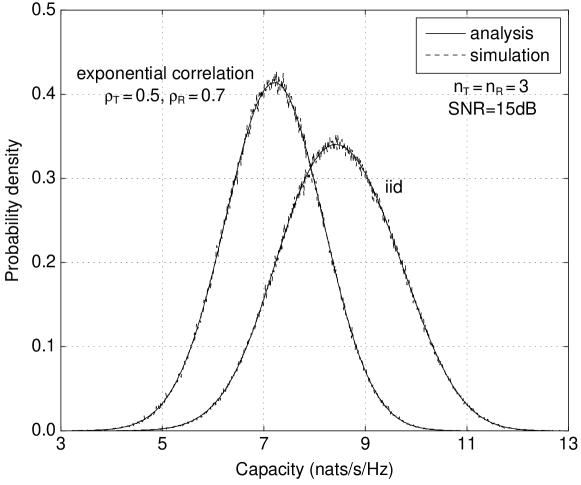
In all examples for exponential correlation, we set ${\mathbf{\Psi}}_{\mathrm{T}}={\mathbf{\Phi}}_{{n_{\mathrm{T}}}}^{\left(\mathrm{exp}\right)}\left({\rho_{\mathrm{T}}}\right)$ and ${\mathbf{\Psi}}_{\mathrm{R}}={\mathbf{\Phi}}_{{n_{\mathrm{R}}}}^{\left(\mathrm{exp}\right)}\left({\rho_{\mathrm{R}}}\right)$. Fig. 1 shows the PDF of $C$ for i.i.d. and exponentially correlated (${\rho_{\mathrm{T}}}=0.5$, ${\rho_{\mathrm{R}}}=0.7$) MIMO channels at $\eta=15$ dB when ${n_{\mathrm{T}}}={n_{\mathrm{R}}}=3$. The analytical curves are plotted by using (1), (9), and [24, eq. (4.33)]. We also compare our analytical results with the simulated PDF obtained by generating $100\,000$ realizations of ${\mathbf{H}}$. It can be seen that analytical and simulated curves match exactly. The figure also shows that the mass of the PDF is mostly above a certain level due to the spatial multiplexing gain (for example, 4 nats/s/Hz for the exponentially correlated case and 5 nats/s/Hz for the i.i.d. case).

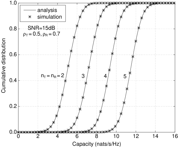
Fig. 2 shows the CDF of $C$ for exponentially correlated MIMO channels with ${\rho_{\mathrm{T}}}=0.5$ and ${\rho_{\mathrm{R}}}=0.7$ at $\eta=15$ dB when ${n_{\mathrm{T}}}={n_{\mathrm{R}}}=2$, $3$, $4$, and $5$. The analytical curves are plotted by using (1) and [24, eq. (4.34)], and they agree exactly with the simulated ones. It can be seen that the capacity increases linearly with the number of antennas for the entire range of cumulative probability, despite the presence of correlation. This can be attributed to the spatial multiplexing gain achieved by increasing the number of antennas at both sides. For example, the capacity at the cumulative probability of $0.1$ (i.e., $10{\%}$ outage capacity) is about $3.76$, $5.95$, $8.12$, and $10.30$ nats/s/Hz for ${n_{\mathrm{T}}}={n_{\mathrm{R}}}=2$, $3$, $4$, and $5$, respectively; we can gain approximately $2.18$ nats/s/Hz of additional capacity for each increase in the number of antennas at both the transmitter and the receiver. Also, the spatial multiplexing gain of MIMO systems guarantees a certain transmission rate at arbitrarily low outage probability (e.g., $2.00$, $4.18$, $6.36$, and $8.54$ nats/s/Hz for ${n_{\mathrm{T}}}={n_{\mathrm{R}}}=2$, $3$, $4$, and $5$, respectively). Fig. 3 illustrates the effect of exponential fading correlation on the capacity distribution for the case of ${n_{\mathrm{T}}}={n_{\mathrm{R}}}=3$ and $\eta=15$ dB, where ${\rho_{\mathrm{T}}}$ and ${\rho_{\mathrm{R}}}$ range from $0$ to $0.9$. It can be seen that the decrease in capacity due to exponential correlation is negligible for a small amount of correlation, but it becomes more significant as the correlation coefficient increases. Moreover, the capacity reduction is more pronounced at high cumulative (or outage) probability.

Fig. 4 shows the analytical and simulated mean, variance, skewness, and kurtosis of $C$ for exponentially correlated MIMO channels as a function of correlation coefficient $\rho$ for ${\rho_{\mathrm{T}}}={\rho_{\mathrm{R}}}=\rho$, ${n_{\mathrm{T}}}={n_{\mathrm{R}}}=3$, and $\eta=15$ dB. Again, our analytical results are in excellent agreement with Monte Carlo simulations that are carried out by generating $100\,000$ realizations of ${\mathbf{H}}$. Fig. 5 shows the mean, variance, skewness, and kurtosis of $C$ versus SNR for i.i.d. and doubly correlated (${\rho_{\mathrm{T}}}=0.5$, ${\rho_{\mathrm{R}}}=0.7$) MIMO channels when ${n_{\mathrm{T}}}={n_{\mathrm{R}}}=2$. It can be seen that as the SNR increases, the variance, skewness, and kurtosis for both i.i.d. and doubly correlated cases converge to $2.290$, $-0.810$, and $1.333$ according to (24), (25), and (31), respectively, and the effect of fading correlation on these statistics diminishes.

V-B METRA Correlation Model

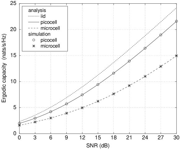
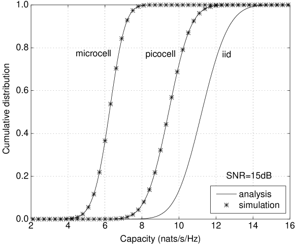
We now consider $4\times 4$ MIMO channels with correlation matrices obtained by the METRA model [17, 18]. In all examples, it can be observed that our analytical results agree exactly with Monte Carlo simulations. Fig. 6 shows the ergodic capacity for METRA correlation matrices, given in [17, p. 82], for picocell and microcell environments. The picocell example is a partially decorrelated scenario selected from a small office environment, whereas the microcell case corresponds to an environment where the receiver (base station) is highly correlated (see [17] for details on the antenna configurations and environment setups). We can see from Fig. 6 that the ergodic capacity at $\eta=15$ dB is $11.25$, $9.44$, and $6.22$ nats/s/Hz for i.i.d., picocell, and microcell cases respectively. The reduction in ergodic capacity due to spatial correlation is about $16\%$ for picocell and $45\%$ for microcell environments, respectively. Fig. 7 shows the CDF of the capacity at $\eta=15$ dB in the same environments as in Fig. 6. The $10\%$ outage capacity is $9.82$, $8.21$, and $5.33$ nats/s/Hz for i.i.d., picocell, and microcell scenarios respectively. The reduction in $10\%$ outage capacity due to spatial correlation is about $16\%$ for picocell and $46\%$ for microcell environments, which is similar to the amount of reduction in ergodic capacity.

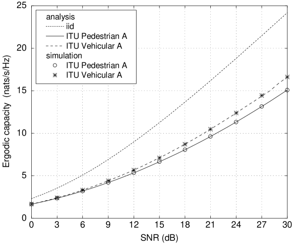
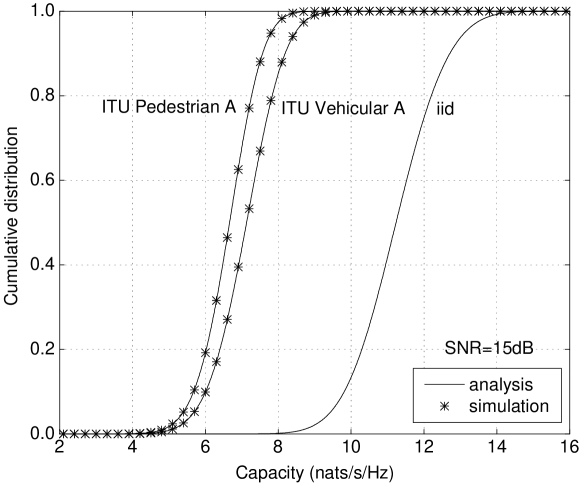
We next consider the METRA correlation matrices, given in [18], for $4\times 4$ MIMO channels in macrocell Pedestrian A and Vehicular A environments of the international telecommunication union (ITU) standard. For these correlation matrices, the ergodic capacity is shown in Fig. 8 and the CDF of the capacity at $\eta=15$ dB is shown in Fig. 9. The ergodic capacity at $\eta=15$ dB is $6.64$ nats/s/Hz for the ITU Pedestrian A and $7.11$ nats/s/Hz for the ITU Vehicular A, respectively (see Fig. 8). Also, $10\%$ outage capacity is $5.67$ and $6.01$ nats/s/Hz for each environment (see Fig. 9). The reduction in ergodic capacity and $10\%$ outage capacity due to spatial correlation is about $40\%$ in both environments.

VI Conclusions

In this paper, we derived closed-form formulas for the exact capacity statistics of Rayleigh-fading MIMO channels in the presence of spatial fading correlation at both the transmitter and the receiver. In particular, we derived the determinant representation for the characteristic function (Theorem 1) and the trace representations for the cumulants (Theorems 2 and 3) of MIMO capacity as well as the mean, variance, skewness, and kurtosis (Tables II and III). These results are valid for arbitrary numbers of antennas, enabling us to calculate both the ergodic capacity and the outage capacity without any approximation and generalizing the previous results for i.i.d. and one-sided correlated MIMO channels. We also showed that in a high-SNR regime, the variance, skewness, kurtosis, and other higher-order statistics of the capacity depend only on correlation at the side with the larger number of antennas. Moreover, when the antenna topology is symmetric (i.e., ${n_{\mathrm{T}}}={n_{\mathrm{R}}})$, these statistics are not affected by fading correlation at any side and the capacity distribution has negative skewness greater than or equal to $-12\sqrt{6}\cdot\zeta\left(3\right)/{\pi^{3}}$, where $\zeta\left(3\right)\approx 1.2020569$ is Apéry’s constant, and positive (excess) kurtosis less than or equal to $2.4$. This implies that the capacity distribution has an asymmetric tail extending out more to the left of the ergodic capacity and a leptokurtic shape more peaked than a Gaussian one. To illustrate our analytical results, we presented numerical examples using the correlation model based on realistic channel measurements as well as the classical exponential correlation model. These examples showed that our analytical results are in excellent agreement with Monte Carlo simulations and that a considerable decrease in capacity, due to spatial fading correlation, can be observed in realistic MIMO channels.

Appendix A: Integral Identities

Let us define the integrals $\mathcal{G}_{n}\left(a,b,\xi\right)$ and $\mathcal{J}_{n,\ell}\left(a,b,\xi\right)$ as

$$\mathcal{G}_{n}\left(a,b,\xi\right)\triangleq\int_{0}^{\infty}\left(1+ax\right)^{\xi-1}x^{n-1}e^{-x/b}dx,\quad a,b>0,~{}n\in\mathbb{N},~{}\xi\in\mathbb{C}$$ (32)

$$\mathcal{J}_{n,\ell}\left(a,b,\xi\right)\triangleq\frac{\partial^{\ell}\mathcal{G}_{n}\left(a,b,\xi\right)}{\partial\xi^{\ell}}=\int_{0}^{\infty}\left(1+ax\right)^{\xi-1}\ln^{\ell}\left(1+ax\right)x^{n-1}e^{-x/b}dx$$ (33)

which appear in deriving the analytical expressions for the capacity statistics in Section III.

From the integral representation of the confluent hypergeometric function $\Psi\left(a,b;z\right)$ in [26, eq. (9.211.4)] and the identity ${}_{2}F_{0}\left(a,b;-z^{-1}\right)=z^{a}\Psi\left(a,a-b+1;z\right)$, the integral $\mathcal{G}_{n}\left(a,b,\xi\right)$ can be evaluated as

$$\mathcal{G}_{n}\left(a,b,\xi\right) =a^{-n}\left(n-1\right)!\Psi\left(n,n+\xi;\frac{1}{ab}\right)$$

$$=b^{n}\left(n-1\right)!\;{}_{2}F_{0}\left(n,-\xi+1;-ab\right)$$ (34)

where ${}_{p}F_{q}\left(a_{1},a_{2},\ldots,a_{p};b_{1},b_{2},\ldots,b_{q};z\right)$ is the generalized hypergeometric function [26, eq. (9.14.1)]. In particular, for $\xi\in\mathbb{N}$, (Appendix A: Integral Identities) reduces to a finite sum of elementary functions as

$$\mathcal{G}_{n}\left(a,b,\xi\right)=b^{n}\sum_{k=0}^{\xi-1}\binom{\xi-1}{k}\left(ab\right)^{k}\left(n+k-1\right)!.$$ (35)

Since the derivatives of the generalized hypergeometric function with respect to its parameters are not known, in general, the integral $\mathcal{J}_{n,\ell}\left(a,b,\xi\right)$ cannot be evaluated directly from (Appendix A: Integral Identities). However, $\mathcal{G}_{n}\left(a,b,\xi\right)$ for $a,b>0$, $n\in\mathbb{N}$ and $\xi\in\mathbb{C}$ can be expressed in an alternate form

$$\mathcal{G}_{n}\left(a,b,\xi\right)=\frac{e^{1/\left(ab\right)}}{a^{n}}\sum_{k=0}^{n-1}\binom{n-1}{k}\left(-1\right)^{n-k-1}\left(ab\right)^{\xi+k}\Gamma\left(\xi+k,\frac{1}{ab}\right)$$ (36)

where $\Gamma\left(\alpha,z\right)=\int_{z}^{\infty}e^{-x}x^{\alpha-1}dx$ is the complementary incomplete gamma function [26, eq. (8.350.2)]. Then, using (36) and Leibniz’s identity [26, p. 21], the integral $\mathcal{J}_{n,\ell}\left(a,b,\xi\right)$ defined in (33) can be evaluated as

$$\mathcal{J}_{n,\ell}\left(a,b,\xi\right) =\frac{e^{1/\left(ab\right)}}{a^{n}}\sum_{k=0}^{n-1}\Biggl{[}\left(-1\right)^{n-k-1}\binom{n-1}{k}\left(ab\right)^{\xi+k}$$

$$\qquad\qquad\qquad\cdot\left.\sum_{i=0}^{\ell}\left\{\binom{\ell}{i}\ln^{\ell-i}\left(ab\right)\cdot\left.\left[\frac{\partial^{i}}{\partial\alpha^{i}}\Gamma\left(\alpha,\frac{1}{ab}\right)\right]\right|_{\alpha=\xi+k}\right\}\right]$$

$$=\frac{\ell!\;e^{1/\left(ab\right)}}{a^{n}}\sum_{k=0}^{n-1}\Biggl{[}\left(-1\right)^{n-k-1}\binom{n-1}{k}\left(ab\right)^{\xi+k}G_{\ell+1,\ell+2}^{\ell+2,0}\Biggl{(}\frac{1}{ab}\Biggm{|}\begin{subarray}{l}\overbrace{1,1,\ldots,1}^{\ell+1\text{ 1's}}\\ \underbrace{0,0,\ldots,0}_{\ell+1\text{ 0's}},\;\text{\normalsize$\xi+k$}\end{subarray}\Biggr{)}\Biggr{]}$$ (37)

where $G_{p,q}^{m,n}\left(\cdot\right)$ is the Meijer G-function [26, eq. (9.301)]. In particular, for $\ell=\xi=1$, (Appendix A: Integral Identities) reduces to

$$\mathcal{J}_{n,1}\left(a,b,1\right)=b^{n}\left(n-1\right)!e^{1/\left(ab\right)}\sum_{k=0}^{n-1}\left(ab\right)^{-k}\Gamma\left(-k,\frac{1}{ab}\right).$$ (38)

Appendix B: Proof of Theorem 1

To proceed with the proof of Theorem 1, we begin by evaluating an integral involving matrix determinants, which is a continuous analogue of the well-known results in multivariate analysis [28]. The next lemma adds a new identity to the list of the generalized Cauchy-Binet formulas derived in [7, Appendix].

Lemma 2

Suppose that $f_{i}$ and $g_{j}$, $i=1,2,\ldots,m$, $j=1,2,\ldots,n$, $m\leq n$, are arbitrary integrable functions over $\mathfrak{D}$. Let ${\mathbf{F}}\left(\varrho_{1},\varrho_{2},\ldots,\varrho_{m}\right)$ and ${\mathbf{G}}\left(\varrho_{1},\varrho_{2},\ldots,\varrho_{m}\right)$ be $m\times m$ and $n\times n$ matrices whose entries depend on $\varrho_{1},\varrho_{2},\ldots,\varrho_{m}$, given by

$$\left\{{\mathbf{F}}\left(\varrho_{1},\varrho_{2},\ldots,\varrho_{m}\right)\right\}_{i,j}=f_{j}\left(\varrho_{i}\right),\qquad i,j=1,2,\ldots,m$$ (39)

$$\left\{{\mathbf{G}}\left(\varrho_{1},\varrho_{2},\ldots,\varrho_{m}\right)\right\}_{i,j}=\begin{cases}c_{i,j},&i=1,\ldots,n-m,~{}j=1,\ldots,n\\[-3.0pt] g_{j}\left(\varrho_{i-n+m}\right),&i=n-m+1,\ldots,n,~{}j=1,\ldots,n\end{cases}$$ (40)

where $c_{i,j}$ are scalar constants. Then,

$$\int_{\mathfrak{D}}\cdots\int_{\mathfrak{D}}\det{\mathbf{F}}\left(\varrho_{1},\varrho_{2},\ldots,\varrho_{m}\right)\det{\mathbf{G}}\left(\varrho_{1},\varrho_{2},\ldots,\varrho_{m}\right)\prod_{\ell=1}^{m}h\left(\varrho_{\ell}\right)d\varrho_{1}d\varrho_{2}\cdots d\varrho_{m}=m!\det\left({\mathbf{\Phi}}\right)$$ (41)

where $h\left(\cdot\right)$ is an arbitrary function and ${\mathbf{\Phi}}$ is the $n\times n$ matrix with $\left(i,j\right)$th entry $\phi_{i,j}$ given by

$$\phi_{i,j}=\begin{cases}c_{i,j},&i=1,\ldots,n-m,~{}j=1,\ldots,n\\[-3.0pt] \int_{\mathfrak{D}}f_{i-n+m}\left(\varrho\right)g_{j}\left(\varrho\right)h\left(\varrho\right)d\varrho,&i=n-m+1,\ldots,n,~{}j=1,\ldots,n.\end{cases}\vspace*{3mm}$$ (42)

Proof:

Let ${\mathbf{a}}=\left(a_{1},a_{2},\ldots,a_{n}\right)$ and ${\mathbf{b}}=\left(b_{1},b_{2},\ldots,b_{m}\right)$ be the permutations of integers $1,2,\ldots,n$ and $1,2,\ldots,m$, respectively. Then, the integration of the left-hand side of (41), denoted by $\mathcal{I}$, becomes

$$\mathcal{I}=\sum_{{\mathbf{b}}}\operatorname{\mathrm{sgn}}\left({\mathbf{b}}\right)\sum_{{\mathbf{a}}}\operatorname{\mathrm{sgn}}\left({\mathbf{a}}\right)\prod_{i=1}^{n-m}c_{i,a_{i}}\prod_{j=1}^{m}\phi_{n-m+b_{j},a_{n-m+j}}\,,$$ (43)

where $\operatorname{\mathrm{sgn}}\left(\cdot\right)$ denotes the sign of the permutation. Note that the sequence $1,2,\ldots,n-m,b_{1}+n-m,b_{2}+n-m,\ldots,b_{m}+n-m$ is a permutation of $1,2,\ldots,n$ with the sign equal to $\operatorname{\mathrm{sgn}}\left({\mathbf{b}}\right)$. Therefore, using [7, eq. (38)], we get

$$\mathcal{I}=\sum_{{\mathbf{b}}}\det\left({\mathbf{\Phi}}\right)=m!\det\left({\mathbf{\Phi}}\right).$$ (44)

∎

Proof of Theorem 1: The CF of $C$ can be written as

$$\Phi_{C}\left({\jmath\omega}\right)=\int_{{\mathbf{\Theta}}={\mathbf{\Theta}}^{\dagger}>0}\det\left({\mathbf{I}}_{n_{\mathrm{S}}}+\bar{\eta}{\mathbf{\Theta}}\right)^{\jmath\omega}p_{{{\mathbf{\Theta}}}}\left({{\mathbf{\Theta}}}\right)d{\mathbf{\Theta}}$$ (45)

where $\bar{\eta}=\eta/{n_{\mathrm{T}}}$ and from (2), the PDF of ${\mathbf{\Theta}}\sim\tilde{Q}_{{{n_{\mathrm{S}}}},{{n_{\mathrm{L}}}}}\left({{\mathbf{I}}_{n_{\mathrm{L}}}},{{\mathbf{\Psi}}_{\mathrm{S}}},{{\mathbf{\Psi}}_{\mathrm{L}}}\right)$ is given by

$$p_{{{\mathbf{\Theta}}}}\left({{\mathbf{\Theta}}}\right)=\frac{1}{\tilde{\Gamma}_{n_{\mathrm{S}}}\left({n_{\mathrm{L}}}\right)}\det\left({\mathbf{\Psi}}_{\mathrm{S}}\right)^{-{n_{\mathrm{L}}}}\det\left({\mathbf{\Psi}}_{\mathrm{L}}\right)^{-{n_{\mathrm{S}}}}\det\left({\mathbf{\Theta}}\right)^{{n_{\mathrm{L}}}-{n_{\mathrm{S}}}}{}_{0}\tilde{F}_{0}^{\left({n_{\mathrm{L}}}\right)}\left(-{\mathbf{\Psi}}_{\mathrm{S}}^{-1}{\mathbf{\Theta}},{\mathbf{\Psi}}_{\mathrm{L}}^{-1}\right).$$ (46)

The typical approach for the evaluation of the integral in (45) is to perform eigenvalue decomposition using the unitary transformation of ${\mathbf{\Theta}}$ and to exploit the knowledge of the joint eigenvalue distribution of ${\mathbf{\Theta}}$. However, the correlation matrix ${\mathbf{\Psi}}_{\mathrm{S}}$ in the argument of the hypergeometric function in (46) prevents the removal of the unitary matrix from its arguments after the eigenvalue decomposition, which makes it difficult to directly use the joint eigenvalue distribution of ${\mathbf{\Theta}}$. We alleviate this difficulty by performing two successive transformations as follows. The first transformation is given by ${\mathbf{Z}}={\mathbf{\Psi}}_{\mathrm{S}}^{-1/2}{\mathbf{\Theta}}{\mathbf{\Psi}}_{\mathrm{S}}^{-1/2}$ with Jacobian $d{\mathbf{\Theta}}=\det\left({\mathbf{\Psi}}_{\mathrm{S}}\right)^{n_{\mathrm{S}}}d{\mathbf{Z}}$. Using the fact that

$${}_{0}\tilde{F}_{0}^{\left({n_{\mathrm{L}}}\right)}\left(-{\mathbf{\Psi}}_{\mathrm{S}}^{-1}{\mathbf{\Theta}},{\mathbf{\Psi}}_{\mathrm{L}}^{-1}\right)={}_{0}\tilde{F}_{0}^{\left({n_{\mathrm{L}}}\right)}\left(-{\mathbf{\Psi}}_{\mathrm{S}}^{-1/2}{\mathbf{\Theta}}{\mathbf{\Psi}}_{\mathrm{S}}^{-1/2},{\mathbf{\Psi}}_{\mathrm{L}}^{-1}\right),$$ (47)

we have

$$\Phi_{C}\left({\jmath\omega}\right)=\frac{\det\left({\mathbf{\Psi}}_{\mathrm{L}}\right)^{-{n_{\mathrm{S}}}}}{\tilde{\Gamma}_{n_{\mathrm{S}}}\left({n_{\mathrm{L}}}\right)}\int_{{\mathbf{Z}}={\mathbf{Z}}^{\dagger}>0} \det\left({\mathbf{I}}_{n_{\mathrm{S}}}+\bar{\eta}{\mathbf{\Psi}}_{\mathrm{S}}{\mathbf{Z}}\right)^{\jmath\omega}$$

$$\cdot\det\left({\mathbf{Z}}\right)^{{n_{\mathrm{L}}}-{n_{\mathrm{S}}}}{}_{0}\tilde{F}_{0}^{\left({n_{\mathrm{L}}}\right)}\left(-{\mathbf{Z}},{\mathbf{\Psi}}_{\mathrm{L}}^{-1}\right)d{\mathbf{Z}}.$$ (48)

Let us denote a unitary manifold of ${n_{\mathrm{S}}}\times{n_{\mathrm{S}}}$ unitary matrices with real diagonal elements by $\tilde{U}\left({n_{\mathrm{S}}}\right)$. Since ${\mathbf{Z}}$ is Hermitian, there exists ${\mathbf{U}}\in\tilde{U}\left({n_{\mathrm{S}}}\right)$ such that ${\mathbf{Z}}={\mathbf{UDU}}^{\dagger}$ and ${\mathbf{D}}=\mathrm{diag}\left(z_{1},z_{2},\ldots,z_{n_{\mathrm{S}}}\right)$ where $0<z_{1}\leq z_{2}\leq\cdots\leq z_{n_{\mathrm{S}}}$ are ordered eigenvalues of ${\mathbf{Z}}$. We then make the second transformation ${\mathbf{Z}}={\mathbf{UDU}}^{\dagger}$ with Jacobian $d{\mathbf{Z}}=\prod_{1\leq i<j\leq{n_{\mathrm{S}}}}\left(z_{j}-z_{i}\right)^{2}d{\mathbf{U}}d{\mathbf{D}}$ [29, Theorem 3.1], [30, Theorem 4.4], yielding

$$\Phi_{C}\left({\jmath\omega}\right)=\frac{\det\left({\mathbf{\Psi}}_{\mathrm{L}}\right)^{-{n_{\mathrm{S}}}}}{\tilde{\Gamma}_{n_{\mathrm{S}}}\left({n_{\mathrm{L}}}\right)}\int_{{\mathbf{D}}} \int_{{\mathbf{U}}\in\tilde{U}{\left({n_{\mathrm{S}}}\right)}}\det\left({\mathbf{I}}_{n_{\mathrm{S}}}+\bar{\eta}{\mathbf{\Psi}}_{\mathrm{S}}{\mathbf{UDU}}^{\dagger}\right)^{\jmath\omega}\det\left({\mathbf{D}}\right)^{{n_{\mathrm{L}}}-{n_{\mathrm{S}}}}$$

$$\qquad\quad\cdot\prod_{1\leq i<j\leq{n_{\mathrm{S}}}}\left(z_{j}-z_{i}\right)^{2}_{0}\tilde{F}_{0}^{\left({n_{\mathrm{L}}}\right)}\left(-{\mathbf{D}},{\mathbf{\Psi}}_{\mathrm{L}}^{-1}\right)d{\mathbf{U}}d{\mathbf{D}}$$ (49)

where we have used the fact that the hypergeometric function with matrix arguments is invariant under unitary transformations of its arguments. It is now apparent that the above two transformations enable us to remove the dependence of ${\mathbf{U}}$ on the hypergeometric function. Recall that the total volume of $\tilde{U}\left({n_{\mathrm{S}}}\right)$ is [30, Corollary 4.3.1]

$$\int_{{\mathbf{U}}\in\tilde{U}\left({n_{\mathrm{S}}}\right)}d{\mathbf{U}}=\frac{\pi^{{n_{\mathrm{S}}}\left({n_{\mathrm{S}}}-1\right)}}{\tilde{\Gamma}_{n_{\mathrm{S}}}\left({n_{\mathrm{S}}}\right)}.$$ (50)

We can now carry out the integration with respect to ${\mathbf{U}}$ using [30, eq. (6.1.19)] and [21, eq. (52)] as

$$\int_{{\mathbf{U}}\in\tilde{U}\left({n_{\mathrm{S}}}\right)}\det\left({\mathbf{I}}_{n_{\mathrm{S}}}+\bar{\eta}{\mathbf{\Psi}}_{\mathrm{S}}{\mathbf{UDU}}^{\dagger}\right)^{\jmath\omega}d{\mathbf{U}}=\frac{\pi^{{n_{\mathrm{S}}}\left({n_{\mathrm{S}}}-1\right)}}{\tilde{\Gamma}_{n_{\mathrm{S}}}\left({n_{\mathrm{S}}}\right)}{}_{1}\tilde{F}_{0}^{\left({n_{\mathrm{S}}}\right)}\left(-\jmath\omega;{\mathbf{D}},-\bar{\eta}{\mathbf{\Psi}}_{\mathrm{S}}\right).$$ (51)

Substituting (51) into (Appendix B: Proof of Theorem 1) gives

$$\Phi_{C}\left({\jmath\omega}\right)= \frac{\pi^{{n_{\mathrm{S}}}\left({n_{\mathrm{S}}}-1\right)}\det\left({\mathbf{\Psi}}_{\mathrm{L}}\right)^{-{n_{\mathrm{S}}}}}{\tilde{\Gamma}_{n_{\mathrm{S}}}\left({n_{\mathrm{L}}}\right)\tilde{\Gamma}_{n_{\mathrm{S}}}\left({n_{\mathrm{S}}}\right)}\int_{0<z_{1}\leq\cdots\leq z_{n_{\mathrm{S}}}<\infty}\prod_{\ell=1}^{n_{\mathrm{S}}}z_{\ell}^{{n_{\mathrm{L}}}-{n_{\mathrm{S}}}}\prod_{1\leq i<j\leq{n_{\mathrm{S}}}}\left(z_{j}-z_{i}\right)^{2}$$

$$\hskip 85.35826pt\cdot{}_{1}\tilde{F}_{0}^{\left({n_{\mathrm{S}}}\right)}\left(-\jmath\omega;{\mathbf{D}},-\bar{\eta}{\mathbf{\Psi}}_{\mathrm{S}}\right){}_{0}\tilde{F}_{0}^{\left({n_{\mathrm{L}}}\right)}\left(-{\mathbf{D}},{\mathbf{\Psi}}_{\mathrm{L}}^{-1}\right)dz_{1}dz_{2}\cdots dz_{n_{\mathrm{S}}}.$$ (52)

Using the results in [23, Lemma 3] and [20], the hypergeometric functions with matrix arguments in the integrand of (Appendix B: Proof of Theorem 1) can be expressed in terms of determinants as

$${}_{1}\tilde{F}_{0}^{\left({n_{\mathrm{S}}}\right)}\left(-\jmath\omega;{\mathbf{D}},-\bar{\eta}{\mathbf{\Psi}}_{\mathrm{S}}\right)=\frac{\left(-\bar{\eta}\pi\right)^{-{n_{\mathrm{S}}}\left({n_{\mathrm{S}}}-1\right)/2}\tilde{\Gamma}_{n_{\mathrm{S}}}\left({n_{\mathrm{S}}}\right)\det\left[\left(1+\bar{\eta}\lambda_{\mathrm{S},{j}}z_{i}\right)^{\jmath\omega+{n_{\mathrm{S}}}-1}\right]_{i,j=1,2,\ldots,{n_{\mathrm{S}}}}}{\prod_{\ell=1}^{n_{\mathrm{S}}}\left(-\jmath\omega-{n_{\mathrm{S}}}+1\right)_{\ell-1}\prod_{1\leq i<j\leq{n_{\mathrm{S}}}}\left(z_{j}-z_{i}\right)\left(\lambda_{\mathrm{S},{j}}-\lambda_{\mathrm{S},{i}}\right)}$$ (53)

$${}_{0}\tilde{F}_{0}^{\left({n_{\mathrm{L}}}\right)}\left(-{\mathbf{D}},{\mathbf{\Psi}}_{\mathrm{L}}^{-1}\right)=\frac{\pi^{-{n_{\mathrm{S}}}\left({n_{\mathrm{S}}}-1\right)/2}\tilde{\Gamma}_{n_{\mathrm{S}}}\left({n_{\mathrm{L}}}\right)\det\left({\mathbf{\Psi}}_{\mathrm{L}}\right)^{n_{\mathrm{S}}}\det\left({\mathbf{\Xi}}\right)}{\prod_{\ell=1}^{n_{\mathrm{S}}}z_{\ell}^{{n_{\mathrm{L}}}-{n_{\mathrm{S}}}}\prod_{1\leq i<j\leq{n_{\mathrm{S}}}}\left(z_{j}-z_{i}\right)\prod_{1\leq i<j\leq{n_{\mathrm{L}}}}\left(\lambda_{\mathrm{L},{j}}-\lambda_{\mathrm{L},{i}}\right)}$$ (54)

where $\left(\alpha\right)_{n}=\alpha\left(\alpha+1\right)\cdots\left(\alpha+n-1\right)$, $\left(\alpha\right)_{0}=1$, is the Pochhammer symbol and ${\mathbf{\Xi}}$ is the ${n_{\mathrm{L}}}\times{n_{\mathrm{L}}}$ matrix whose $\left(i,j\right)$th entry is given by

$$\left\{{\mathbf{\Xi}}\right\}_{i,j}=\begin{cases}\lambda_{\mathrm{L},{j}}^{i-1},&i=1,\ldots,{n_{\mathrm{L}}}-{n_{\mathrm{S}}},~{}j=1,\ldots,{n_{\mathrm{L}}}\\ \lambda_{\mathrm{L},{j}}^{{n_{\mathrm{L}}}-{n_{\mathrm{S}}}-1}\exp\left(-\frac{z_{i-{n_{\mathrm{L}}}+{n_{\mathrm{S}}}}}{\lambda_{\mathrm{L},{j}}}\right),&i={n_{\mathrm{L}}}-{n_{\mathrm{S}}}+1,\ldots,{n_{\mathrm{L}}},~{}j=1,\ldots,{n_{\mathrm{L}}}.\end{cases}$$ (55)

Combining (Appendix B: Proof of Theorem 1)–(55) together with

$$\left(-1\right)^{{n_{\mathrm{S}}}\left({n_{\mathrm{S}}}-1\right)/2}\prod_{\ell=1}^{n_{\mathrm{S}}}\left(-\jmath\omega-{n_{\mathrm{S}}}+1\right)_{\ell-1}=\prod_{\ell=1}^{{n_{\mathrm{S}}}-1}\left(\jmath\omega+\ell\right)^{\ell},$$ (56)

we get

$$\Phi_{C}\left({\jmath\omega}\right) =\frac{\Upsilon_{n_{\mathrm{S}}}\left(\jmath\omega\right)}{K_{\mathrm{cor}}}\int_{0<z_{1}\leq\cdots\leq z_{n_{\mathrm{S}}}<\infty}\det\left[\left(1+\bar{\eta}\lambda_{\mathrm{S},{j}}z_{i}\right)^{\jmath\omega+{n_{\mathrm{S}}}-1}\right]_{i,j=1,2,\ldots,{n_{\mathrm{S}}}}\det\left({\mathbf{\Xi}}\right)dz_{1}\cdots dz_{n_{\mathrm{S}}}$$

$$=\frac{\Upsilon_{n_{\mathrm{S}}}\left(\jmath\omega\right)}{{n_{\mathrm{S}}}!K_{\mathrm{cor}}}\int_{0}^{\infty}\cdots\int_{0}^{\infty}\det\left[\left(1+\bar{\eta}\lambda_{\mathrm{S},{j}}z_{i}\right)^{\jmath\omega+{n_{\mathrm{S}}}-1}\right]_{i,j=1,2,\ldots,{n_{\mathrm{S}}}}\det\left({\mathbf{\Xi}}\right)dz_{1}\cdots dz_{n_{\mathrm{S}}}$$ (57)

where the last equality follows from the fact that the integrand is symmetric in $z_{1},z_{2},\ldots,z_{n_{\mathrm{S}}}$. Finally, applying the integral-type Cauchy-Binet formula in Lemma 2 to (Appendix B: Proof of Theorem 1) and using the identity (Appendix A: Integral Identities) complete the proof.

TABLE I: Some matrices involved in the analytical expressions for the capacity statistics (see Appendix A for details on the evaluation of integrals). Denote $~{}\bar{\eta}=\eta/{n_{\mathrm{T}}}$.

Notation	Dimension	$~{}\left(i,j\right)$th entry (where $\imath=i-{n_{\mathrm{L}}}+{n_{\mathrm{S}}}$ and $n\in\mathbb{N}$)
${\mathbf{\Lambda}}\left(\nu\right)$	${n_{\mathrm{L}}}\times{n_{\mathrm{L}}}$	$\begin{array}[]{l}\left\{{\mathbf{\Lambda}}\left(\nu\right)\right\}_{i=1,2,\dots,{n_{\mathrm{L}}}-{n_{\mathrm{S}}},j=1,2,\dots,{n_{\mathrm{L}}}}=\lambda_{\mathrm{L},{j}}^{i-1}\\ \left\{{\mathbf{\Lambda}}\left(\nu\right)\right\}_{i={n_{\mathrm{L}}}-{n_{\mathrm{S}}}+1,{n_{\mathrm{L}}}-{n_{\mathrm{S}}}+2,\dots,{n_{\mathrm{L}}},j=1,2,\dots,{n_{\mathrm{L}}}}\\ \quad=\displaystyle{\lambda_{\mathrm{L},{j}}^{{n_{\mathrm{L}}}-{n_{\mathrm{S}}}-1}\int_{0}^{\infty}\left(1+\bar{\eta}\lambda_{\mathrm{S},{\imath}}z\right)^{\nu+{n_{\mathrm{S}}}-1}e^{-z/\lambda_{\mathrm{L},{j}}}dz}\\ \quad=\lambda_{\mathrm{L},{j}}^{{n_{\mathrm{L}}}-{n_{\mathrm{S}}}}\;{}_{2}F_{0}\left(1,-\nu-{n_{\mathrm{S}}}+1;-\bar{\eta}\lambda_{\mathrm{S},{\imath}}\lambda_{\mathrm{L},{j}}\right)\end{array}$
${\mathbf{\Lambda}}^{\left(n\right)}\left(\nu\right)$	${n_{\mathrm{L}}}\times{n_{\mathrm{L}}}$	$\begin{array}[]{l}\left\{{\mathbf{\Lambda}}^{\left(n\right)}\left(\nu\right)\right\}_{i=1,2,\dots,{n_{\mathrm{L}}}-{n_{\mathrm{S}}},j=1,2,\dots,{n_{\mathrm{L}}}}=0\\ \left\{{\mathbf{\Lambda}}^{\left(n\right)}\left(\nu\right)\right\}_{i={n_{\mathrm{L}}}-{n_{\mathrm{S}}}+1,{n_{\mathrm{L}}}-{n_{\mathrm{S}}}+2,\dots,{n_{\mathrm{L}}},j=1,2,\dots,{n_{\mathrm{L}}}}\\ \quad=\displaystyle{\lambda_{\mathrm{L},{j}}^{{n_{\mathrm{L}}}-{n_{\mathrm{S}}}-1}\int_{0}^{\infty}\left(1+\bar{\eta}\lambda_{\mathrm{S},{\imath}}z\right)^{\nu+{n_{\mathrm{S}}}-1}\ln^{n}\left(1+\bar{\eta}\lambda_{\mathrm{S},{\imath}}z\right)e^{-z/\lambda_{\mathrm{L},{j}}}dz}\\ \quad=n!\left(\bar{\eta}\lambda_{\mathrm{S},{\imath}}\right)^{\nu+{n_{\mathrm{S}}}-1}\lambda_{\mathrm{L},{j}}^{\nu+{n_{\mathrm{L}}}-1}\exp\left(\frac{1}{\bar{\eta}\lambda_{\mathrm{S},{\imath}}\lambda_{\mathrm{L},{j}}}\right)\\ \qquad\times G_{n+1,n+2}^{n+2,0}\left(\left.\frac{1}{\bar{\eta}\lambda_{\mathrm{S},{\imath}}\lambda_{\mathrm{L},{j}}}\right|\begin{subarray}{l}1,1,\ldots,1\\ 0,0,\ldots,0,\nu+{n_{\mathrm{S}}}\end{subarray}\right)\end{array}$
${\mathbf{\Omega}}\left(\nu\right)$	${n_{\mathrm{S}}}\times{n_{\mathrm{S}}}$	$\begin{array}[]{l}\left\{{\mathbf{\Omega}}\left(\nu\right)\right\}_{i,j=1,2,\ldots,{n_{\mathrm{S}}}}\\ \quad=\displaystyle{\int_{0}^{\infty}\left(1+\bar{\eta}z\right)^{\nu}z^{{n_{\mathrm{L}}}-{n_{\mathrm{S}}}+i+j-2}e^{-z}dz}\\ \quad=\left({n_{\mathrm{L}}}-{n_{\mathrm{S}}}+i+j-2\right)!\;{}_{2}F_{0}\left({n_{\mathrm{L}}}-{n_{\mathrm{S}}}+i+j-1,-\nu;-\bar{\eta}\right)\end{array}$
${\mathbf{\Omega}}^{\left(n\right)}\left(\nu\right)$	${n_{\mathrm{S}}}\times{n_{\mathrm{S}}}$	$\begin{array}[]{l}\left\{{\mathbf{\Omega}}^{\left(n\right)}\left(\nu\right)\right\}_{i,j=1,2,\ldots,{n_{\mathrm{S}}}}\\ \quad=\displaystyle{\int_{0}^{\infty}\left(1+\bar{\eta}z\right)^{\nu}\ln^{n}\left(1+\bar{\eta}z\right)z^{{n_{\mathrm{L}}}-{n_{\mathrm{S}}}+i+j-2}e^{-z}dz}\\ \quad=\displaystyle{\frac{n!e^{1/\bar{\eta}}}{\bar{\eta}^{{n_{\mathrm{L}}}-{n_{\mathrm{S}}}+i+j-1}}\sum_{k=0}^{{n_{\mathrm{L}}}-{n_{\mathrm{S}}}+i+j-2}\Biggl{[}\left(-1\right)^{{n_{\mathrm{L}}}-{n_{\mathrm{S}}}+i+j-k-2}}\\ \qquad\times\binom{{n_{\mathrm{L}}}-{n_{\mathrm{S}}}+i+j-2}{k}\bar{\eta}^{\nu+k+1}G_{n+1,n+2}^{n+2,0}\left(\left.\frac{1}{\bar{\eta}}\right|\begin{subarray}{l}1,1,\ldots,1\\ 0,0,\ldots,0,\nu+k+1\end{subarray}\right)\Biggr{]}\end{array}$

TABLE II: Mean, variance, skewness, and kurtosis of the capacity in nats/s/Hz for i.i.d. MIMO channels, ${\mathbf{H}}\sim\tilde{\mathcal{N}}_{{{n_{\mathrm{R}}}},{{n_{\mathrm{T}}}}}\left({{\mathbf{0}}},{{\mathbf{I}}_{n_{\mathrm{R}}}},{{\mathbf{I}}_{n_{\mathrm{T}}}}\right).~{}$ Denote $~{}{\mathbf{\Omega}}_{n}={\mathbf{\Omega}}_{[n]}\left(0\right)$.

	$m_{1}$ (mean)	$\operatorname{\mathrm{tr}}\left({\mathbf{\Omega}}_{1}\right)$
	$\mu_{2}$ (variance)	$\operatorname{\mathrm{tr}}\left({\mathbf{\Omega}}_{2}-{\mathbf{\Omega}}_{1}^{2}\right)$
	$\beta_{1}$ (skewness)	$\displaystyle{\frac{\operatorname{\mathrm{tr}}\left(2\,{\mathbf{\Omega}}_{1}^{3}-3\,{\mathbf{\Omega}}_{1}{\mathbf{\Omega}}_{2}+{\mathbf{\Omega}}_{3}\right)}{\left[\operatorname{\mathrm{tr}}\left({\mathbf{\Omega}}_{2}-{\mathbf{\Omega}}_{1}^{2}\right)\right]^{3/2}}}$
	$\beta_{2}$ (kurtosis)	$\displaystyle{\frac{\operatorname{\mathrm{tr}}\left(-6\,{\mathbf{\Omega}}_{1}^{4}+12\,{\mathbf{\Omega}}_{1}^{2}\,{\mathbf{\Omega}}_{2}-3\,{\mathbf{\Omega}}_{2}^{2}-4\,{\mathbf{\Omega}}_{1}{\mathbf{\Omega}}_{3}+{\mathbf{\Omega}}_{4}\right)}{\left[\operatorname{\mathrm{tr}}\left({\mathbf{\Omega}}_{2}-{\mathbf{\Omega}}_{1}^{2}\right)\right]^{2}}}$

TABLE III: Mean, variance, skewness, and kurtosis of the capacity in nats/s/Hz for doubly correlated MIMO channels, $~{}{\mathbf{H}}\sim\tilde{\mathcal{N}}_{{{n_{\mathrm{R}}}},{{n_{\mathrm{T}}}}}\left({{\mathbf{0}}},{{\mathbf{\Psi}}_{\mathrm{R}}},{{\mathbf{\Psi}}_{\mathrm{T}}}\right).~{}$ Denote $~{}{\mathbf{\Lambda}}_{n}={\mathbf{\Lambda}}_{[n]}\left(0\right)$.

	$m_{1}$ (mean)	$\operatorname{\mathrm{tr}}\left({\mathbf{\Lambda}}_{1}\right)-\left({n_{\mathrm{S}}}-1\right)$
	$\mu_{2}$ (variance)	$\displaystyle{\operatorname{\mathrm{tr}}\left({\mathbf{\Lambda}}_{2}-{\mathbf{\Lambda}}_{1}^{2}\right)+\sum_{\ell=1}^{{n_{\mathrm{S}}}-1}\ell^{-1}}$
	$\beta_{1}$ (skewness)	$\displaystyle{\frac{\operatorname{\mathrm{tr}}\left(2{\mathbf{\Lambda}}_{1}^{3}-3{\mathbf{\Lambda}}_{1}{\mathbf{\Lambda}}_{2}+{\mathbf{\Lambda}}_{3}\right)-\sum_{\ell=1}^{{n_{\mathrm{S}}}-1}2\ell^{-2}}{\left[\operatorname{\mathrm{tr}}\left({\mathbf{\Lambda}}_{2}-{\mathbf{\Lambda}}_{1}^{2}\right)+\sum_{\ell=1}^{{n_{\mathrm{S}}}-1}\ell^{-1}\right]^{3/2}}}$
	$\beta_{2}$ (kurtosis)	$\displaystyle{\frac{\operatorname{\mathrm{tr}}\left(-6{\mathbf{\Lambda}}_{1}^{4}+12{\mathbf{\Lambda}}_{1}^{2}{\mathbf{\Lambda}}_{2}-3{\mathbf{\Lambda}}_{2}^{2}-4{\mathbf{\Lambda}}_{1}{\mathbf{\Lambda}}_{3}+{\mathbf{\Lambda}}_{4}\right)+\sum_{\ell=1}^{{n_{\mathrm{S}}}-1}6\ell^{-3}}{\left[\operatorname{\mathrm{tr}}\left({\mathbf{\Lambda}}_{2}-{\mathbf{\Lambda}}_{1}^{2}\right)+\sum_{\ell=1}^{{n_{\mathrm{S}}}-1}\ell^{-1}\right]^{2}}}$

Figure 1: PDF of the capacity for i.i.d. and exponentially correlated (${\rho_{\mathrm{T}}}=0.5$, ${\rho_{\mathrm{R}}}=0.7$) MIMO channels. ${n_{\mathrm{T}}}={n_{\mathrm{R}}}=3$ and $\eta=15$ dB.

Figure 2: CDF of the capacity for exponentially correlated MIMO channels with ${\rho_{\mathrm{T}}}=0.5$ and ${\rho_{\mathrm{R}}}=0.7$. ${n_{\mathrm{T}}}={n_{\mathrm{R}}}=2,3,4,5$ and $\eta=15$ dB.

Figure 3: CDF of the capacity for exponentially correlated MIMO channels with ${\rho_{\mathrm{T}}}={\rho_{\mathrm{R}}}=0$ (i.i.d.), $0.1,0.2,0.3,0.4,0.5,0.6$, $0.7,0.8$, and $0.9$. ${n_{\mathrm{T}}}={n_{\mathrm{R}}}=3$ and $\eta=15$ dB.

Figure 4: Mean, variance, skewness, and kurtosis of the capacity (nats/s/Hz) as a function of correlation coefficient $\rho$ for exponentially correlated MIMO channels with ${\rho_{\mathrm{T}}}={\rho_{\mathrm{R}}}=\rho$. ${n_{\mathrm{T}}}={n_{\mathrm{R}}}=3$ and $\eta=15$ dB.

Figure 5: Mean, variance, skewness, and kurtosis of the capacity (nats/s/Hz) versus SNR for i.i.d. and doubly correlated (${\rho_{\mathrm{T}}}=0.5$, ${\rho_{\mathrm{R}}}=0.7$) MIMO channels. ${n_{\mathrm{T}}}={n_{\mathrm{R}}}=2$.

Figure 6: Ergodic capacity of doubly correlated MIMO channels with ${n_{\mathrm{T}}}={n_{\mathrm{R}}}=4$ and METRA correlation matrices given in [17, p. 82] for picocell and microcell environments. For comparison, the ergodic capacity of the $4\times 4$ i.i.d. MIMO channel is also plotted.

Figure 7: CDF of the capacity for doubly correlated MIMO channels with ${n_{\mathrm{T}}}={n_{\mathrm{R}}}=4$ and METRA correlation matrices given in [17, p. 82] for picocell and microcell environments. For comparison, the CDF of capacity for the $4\times 4$ i.i.d. MIMO channel is also plotted. $\eta=15$ dB.

Figure 8: Ergodic capacity of doubly correlated MIMO channels with ${n_{\mathrm{T}}}={n_{\mathrm{R}}}=4$ and METRA correlation matrices given in [18] for macrocell ITU Pedestrian A and Vehicular A environments. For comparison, the ergodic capacity of the $4\times 4$ i.i.d. MIMO channel is also plotted.

Figure 9: CDF of the capacity for doubly correlated MIMO channels with ${n_{\mathrm{T}}}={n_{\mathrm{R}}}=4$ and METRA correlation matrices given in [18] for macrocell ITU Pedestrian A and Vehicular A environments. For comparison, the CDF of capacity for the $4\times 4$ i.i.d. MIMO channel is also plotted. $\eta=15$ dB.

References

• [1] J. H. Winters, “On the capacity of radio communication systems with diversity in Rayleigh fading environment,” IEEE J. Select. Areas Commun., vol. 5, no. 5, pp. 871–878, June 1987.
• [2] G. J. Foschini and M. J. Gans, “On limits of wireless communications in a fading environment when using multiple antennas,” Wireless Personal Commun., vol. 6, no. 3, pp. 311–335, Mar. 1998.
• [3] İ. E. Telatar, “Capacity of multi-antenna Gaussian channels,” European Trans. Telecommun., vol. 10, no. 6, pp. 585–595, Nov./Dec. 1999.
• [4] D.-S. Shiu, G. J. Foschini, M. J. Gans, and J. M. Kahn, “Fading correlation and its effect on the capacity of multielement antenna systems,” IEEE Trans. Commun., vol. 48, no. 3, pp. 502–513, Mar. 2000.
• [5] C.-N. Chuah, D. N. C. Tse, J. M. Kahn, and R. A. Valenzuela, “Capacity scaling in MIMO wireless systems under correlated fading,” IEEE Trans. Inform. Theory, vol. 48, no. 3, pp. 637–650, Mar. 2002.
• [6] H. Shin and J. H. Lee, “Capacity of multiple-antenna fading channels: Spatial fading correlation, double scattering, and keyhole,” IEEE Trans. Inform. Theory, vol. 49, no. 10, pp. 2636–2647, Oct. 2003.
• [7] M. Chiani, M. Z. Win, and A. Zanella, “On the capacity of spatially correlated MIMO Rayleigh-fading channels,” IEEE Trans. Inform. Theory, vol. 49, no. 10, pp. 2363–2371, Oct. 2003.
• [8] P. J. Smith, S. Roy, and M. Shafi, “Capacity of MIMO systems with semicorrelated flat fading,” IEEE Trans. Inform. Theory, vol. 49, no. 10, pp. 2781–2788, Oct. 2003.
• [9] M. Kang and M.-S. Alouini, “Impact of correlation on the capacity of MIMO channels,” in Proc. IEEE Int. Conf. Communications (ICC’03), Anchorage, AK, May 2003, pp. 2623–2627.
• [10] P. J. Smith, L. M. Garth, and S. Loyka, “Exact capacity distributions for MIMO systems with small numbers of antennas,” IEEE Commun. Lett., vol. 7, no. 10, pp. 481–483, Oct. 2003.
• [11] A. Giorgetti, P. J. Smith, M. Shafi, and M. Chiani, “MIMO capacity, level crossing rates and fades: The impact of spatial/temporal channel correlation,” J. Communications and Networks, vol. 5, no. 2, pp. 104–115, June 2003.
• [12] Ö. Oyman, R. U. Nabar, H. Bolcskei, and A. J. Paulraj, “Characterizing the statistical properties of mutual information in MIMO channels,” IEEE Trans. Signal Processing, vol. 51, no. 11, pp. 2784–2795, Nov. 2003.
• [13] A. L. Moustakas, S. H. Simon, and A. M. Sengupta, “MIMO capacity through correlated channels in the presence of correlated interferers and noise: A (not so) large N𝑁{N} analysis,” IEEE Trans. Inform. Theory, vol. 49, no. 10, pp. 2545–2561, Oct. 2003.
• [14] C. Martin and B. Ottersten, “Asymptotic eigenvalue distributions and capacity for MIMO channels under correlated fading,” IEEE Trans. Wireless Commun., vol. 3, no. 4, pp. 1350–1359, July 2004.
• [15] E. Biglieri, J. Proakis, and S. Shamai (Shitz), “Fading channels: Information-theoretic and communications aspects,” IEEE Trans. Inform. Theory, vol. 44, no. 6, pp. 2619–2692, Oct. 1998.
• [16] P. J. Smith and M. Shafi, “An approximate capacity distribution for MIMO systems,” IEEE Trans. Commun., vol. 52, no. 6, pp. 887–890, June 2004.
• [17] J. P. Kermoal, “Measurement, modelling and performance evaluation of the MIMO radio channel,” Ph.D. dissertation, Aalborg University, Aalorg, Denmark, Aug. 2002.
• [18] C802.20-03/50. (2003, May) Overview of METRA model for MBWA MIMO channel. This document has been prepared to assist the IEEE 802.20 Working Group. IEEE 802.20 Session#2. [Online]. Available: http://www.ieee802.org/20/Contribs/C802.20-03-50.doc
• [19] M. Kiessling, “Unifying analysis of ergodic MIMO capacity in correlated Rayleigh fading environments,” European Trans. Telecommun., vol. 16, no. 1, pp. 17–35, Jan./Feb. 2005.
• [20] H. Gao and P. J. Smith, “A determinant representation for the distribution of quadratic forms in complex normal vectors,” J. Multivariate Analysis, vol. 73, pp. 155–165, 2000.
• [21] C. G. Khatri, “On certain distribution problems based on positive definite quadratic functions in normal vectors,” Ann. Math. Statistics, vol. 37, no. 2, pp. 468–479, Apr. 1966.
• [22] A. K. Gupta and D. K. Nagar, Matrix Variate Distributions.   Boca Raton, FL: Chapman & Hall/CRC, 2000.
• [23] C. G. Khatri, “On the moments of traces of two matrices in three situations for complex multivariate normal populations,” Sankhya, The Indian J. Statistics, Series A, vol. 32, pp. 65–80, Mar. 1970.
• [24] H. Shin, “Capacity and error exponents for multiple-input multiple-output wireless channels,” Ph.D. dissertation, Seoul National University, Seoul, Korea, Aug. 2004.
• [25] M. A. Golberg, “The derivative of a determinant,” American Math. Monthly, vol. 79, no. 10, pp. 1124–1126, Dec. 1972.
• [26] I. S. Gradshteyn and I. M. Ryzhik, Table of Integrals, Series, and Products, 6th ed.   San Diego, CA: Academic, 2000.
• [27] M. Evans, N. Hastings, and B. Peacock, Statistical Distributions, 3rd ed.   New York: Wiley, 2000.
• [28] P. R. Krishnaiah, “Some recent developments on complex multivariate distributions,” J. Multivariate Analysis, vol. 6, pp. 1–30, 1976.
• [29] A. Edelman, “Eigenvalues and condition numbers of random matrices,” Ph.D. dissertation, M.I.T., Cambridge, MA, May 1989.
• [30] A. M. Mathai, Jacobians of Matrix Transformations and Functions of Matrix Arguments.   Singapore: World Scientific, 1997.