Grid Vertex-Unfolding Orthogonal Polyhedra

Abstract

An edge-unfolding of a polyhedron is produced by cutting along edges and flattening the faces to a net, a connected planar piece with no overlaps. A grid unfolding allows additional cuts along grid edges induced by coordinate planes passing through every vertex. A vertex-unfolding permits faces in the net to be connected at single vertices, not necessarily along edges. We show that any orthogonal polyhedra of genus zero has a grid vertex-unfolding. (There are orthogonal polyhedra that cannot be vertex-unfolded, so some type of “gridding” of the faces is necessary.) For any orthogonal polyhedron $P$ with $n$ vertices, we describe an algorithm that vertex-unfolds $P$ in $O(n^{2})$ time. Enroute to explaining this algorithm, we present a simpler vertex-unfolding algorithm that requires a $3\times 1$ refinement of the vertex grid.

Keywords:

vertex-unfolding, grid unfolding, orthogonal polyhedra, genus-zero.

1 Introduction

Two unfolding problems have remained unsolved for many years [DO05a]: (1) Can every convex polyhedron be edge-unfolded? (2) Can every polyhedron be unfolded? An unfolding of a 3D object is an isometric mapping of its surface to a single, connected planar piece, the “net” for the object, that avoids overlap. An edge-unfolding achieves the unfolding by cutting edges of a polyhedron, whereas a general unfolding places no restriction on the cuts. A net representation of a polyhedron finds use in a variety of applications [O’R00] — from flattening monkey brains [SSW89] to manufacturing from sheet metal [Wan97] to low-distortion texture mapping [THCM04].

It is known that some nonconvex polyhedra cannot be unfolded without overlap with cuts along edges. However, no example is known of a nonconvex polyhedron that cannot be unfolded with unrestricted cuts. Advances on these difficult problems have been made by specializing the class of polyhedra, or easing the stringency of the unfolding criteria. On one hand, it was established in [BDD⁺98] that certain subclasses of orthogonal polyhedra — those whose faces meet at angles that are multiples of $90^{\circ}$ — have an unfolding. In particular, the class of orthostacks, stacks of extruded orthogonal polygons, was proven to have an unfolding (but not an edge-unfolding). On the other hand, loosening the criteria of what constitutes a net to permit connection through points/vertices, the so-called vertex-unfoldings, led to an algorithm to vertex-unfold any triangulated manifold [DEE⁺03] (and indeed, any simplicial manifold in higher dimensions). A vertex unfolding maps the surface to a single, connected piece $P$ in the plane, but $P$ may have “cut vertices” whose removal disconnect $P$.

A second loosening of the criteria is the notion of grid unfoldings, which are especially natural for orthogonal polyhedra. A grid unfolding adds edges to the surface by intersecting the polyhedron with planes parallel to Cartesian coordinate planes through every vertex. The two approaches were recently married in [DIL04], which established that any orthostack may be grid vertex-unfolded. For orthogonal polyhedra, a grid unfolding is a natural median between edge-unfoldings and unrestricted unfoldings.

Our main result is that any orthogonal polyhedron, without shape restriction except that its surface be homeomorphic to a sphere, has a grid vertex-unfolding. We present an algorithm that grid vertex-unfolds any orthogonal polyhedron with $n$ vertices in $O(n^{2})$ time. We also present, along the way, a simpler algorithm for $3\times 1$ refinement unfolding, a weakening of grid unfolding that we define below. We believe that the techniques in our algorithms may help show that all orthogonal polyhedra can be grid edge-unfolded.

2 Definitions

A $k_{1}\times k_{2}$ refinement of a surface [DO05b] partitions each face into a $k_{1}\times k_{2}$ grid of faces. We will consider refinements of grid unfoldings, with the convention that a $1\times 1$ refinement is an unrefined grid unfolding.

We distinguish between a strict net, in which the net boundary does not self-touch, and a net for which the boundary may touch, but no interior points overlap. The latter corresponds to the physical model of cutting out the net from a sheet of paper, with perhaps some cuts representing edge overlap, and this is the model we use in this paper. We also insist as part of the definition of a vertex-unfolding, again keeping in spirit with the physical model, that the unfolding “path” never self-crosses on the surface in the following sense. If $(A,B,C,D)$ are four faces incident in that cyclic order to a common vertex $v$, then the net does not include both the connections $AvC$ and $BvD$.

We use the following notation to describe the six type of faces of an orthogonal polyhedron, depending on the direction in which the outward normal points: front: $-y$; back: $+y$; left: $-x$; right: $+x$; bottom: $-z$; top: $+z$. We take the $z$-axis to define the vertical direction; vertical faces are parallel to the $xz$-plane. Directions clockwise (cw), and counterclockwise (ccw) are defined from the perspective of a viewer positioned at $y=-\infty$. We distinguish between an original vertex of the polyhedron, which we call a corner vertex or just a vertex, and a gridpoint, a vertex of the grid (which might be an original vertex). A gridedge is an edge segment with both endpoint gridpoints, and a gridface is a face of the grid bounded by gridedges.

Let $O$ be a solid orthogonal polyhedron with the surface homeomorphic to a sphere (i.e, genus zero). Let $Y_{i}$ be the plane $y=y_{i}$ orthogonal to the $y$-axis. Let $Y_{0},Y_{1},\ldots,Y_{i},\ldots$ be a finite sequence of parallel planes passing through every vertex of $O$, with $y_{0}<y_{1}<\cdots<y_{i}<\cdots$. We define layer $i$ to be the portion of $O$ between planes $Y_{i}$ and $Y_{i+1}$. Observe that a layer may include a collection of disjoint connected components of $O$; we call each such component a slab. A surface piece that surrounds a slab is called a band. Referring to Fig. 1a, layer $0$, $1$ and $2$ each contain one slab (with outer bands $A$, $B$ and $D$, respectively). Note that each slab is bounded by an outer (surface) band, but it may also contain inner bands, bounding holes. Outer bands are called protrusions and inner bands are called dents ($C$ in Fig. 1a). In other words, band $A$ is a protrusion if a traversal of the rim of $A$ in $Y_{i}$, ccw from the viewpoint of $y=-\infty$, has the interior of $O$ to the left of $A$, and a dent if this traversal has the interior of $O$ to the right.

For fixed $i$, define $P=\partial O\cap Y_{i}$ as the portion of the surface of $O$ lying in plane $Y_{i}$. $P^{+}$ is the portion of $P$ with normal in the direction $+y$ (composed of back faces), and $P^{-}$ the portion with normal in the direction $-y$ (composed of front faces). By convention, band points in $P$ that are not incident to either front or back faces (e.g., when one band aligns with another), belong to both $P^{+}$ and $P^{-}$. Thus $P=P^{+}\cup P^{-}$.

For a band $A$, Let $R_{i}(A)=A\cap Y_{i}$ be the polygon in $Y_{i}$ determined by the rim of band $A$, and $r_{i}(A)$ the closed region of $Y_{i}$ whose boundary is $R_{i}(A)$. For any two bands $A$ and $B$, let $r_{i}(AB)=r_{i}(A)\cap r_{i}(B)$ and let $R_{i}(AB)$ be the boundary of $r_{i}(AB)$.

Figure 1: Definitions. (a) Shaded connected pieces are bands; $A$, $B$ and $D$ are protrusions; $C$ is a dent; $r_{2}(CB)$ coincides with the back face of $C$; $R_{2}(DB)$ is marked in dashed lines. (b) The adjacency structure of bands is a tree.

3 Dents vs. Protrusions

We observe that dents may be treated exactly the same as protrusions with respect to unfolding, because an unfolding of a $2$-manifold to another surface (in our case, a plane) depends only on the intrinsic geometry of the surface, and not on how it is embedded in $\mathbb{R}^{3}$. Note that we are only concerned with the final unfolded “flat state” [DO05a], and not with possible intersections during a continuous sequence of partially unfolded intermediate states. Our unfolding algorithm relies solely on the amount of surface material surrounding each point: the cyclic ordering of the faces incident to a vertex, and the pair of faces sharing an edge. All these local relationships remain unchanged if we conceptually “pop-out” dents to become protrusions, i.e., a “Flatland” creature living in the surface could not tell the difference; nor can our algorithm. We note that the popping-out is conceptual only, for it could produce self-intersecting objects. Also dents are gridded independently of the rest of the object, so that it would not matter whether they are popped out or not.

Although the dent/protrusion distinction is irrelevant to the unfolding, the interrelationships between dents and protrusions touching a particular $Y_{i}$ do depend on this distinction. To cite just the simplest example, there cannot be two nested protrusions to the same side of $Y_{i}$, but a protrusion could have a dent in it to the same side of $Y_{i}$ (e.g., protrusion $B$ encloses dent $C$ to the same side of $Y_{1}$ in Fig. 1). These relationships are crucial to the connectivity of the band graph $G_{b}$, discussed in Sec. 8.

4 Overview

The two algorithms we present share a common central structure, with the second achieving a stronger result; both are vertex-unfoldings that use orthogonal cuts only. We note that it is the restriction to orthogonal cuts that makes the vertex-unfolding problem difficult: if arbitrary cuts are allowed, then a general vertex-unfolding can be obtained by simply triangulating each face and applying the algorithm from [DEE⁺03].

The ($3\times 1$)-algorithm unfolds any genus-0 orthogonal polyhedron that has been refined in one direction 3-fold. The bands themselves are never split (unlike in [BDD⁺98]). The algorithm is simple. The ($1\times 1$)-algorithm also unfolds any genus-0 orthogonal polyhedron, but this time achieving a grid vertex-unfolding, i.e., without refinement. This algorithm is more delicate, with several cases not present in the ($3\times 1$)-algorithm that need careful detailing. Clearly this latter algorithm is stronger, and we vary the detail of presentation to favor it. The overall structure of the two algorithms is the same:

1. A band “unfolding tree” $T_{U}$ is constructed by shooting rays vertically from the top of bands. The root of $T_{U}$ is a frontmost band (of smallest $y$-coordinate), with ties broken arbitrarily.

2. A forward and return connecting path of vertical faces is identified, each of which connects a parent band to a child band in $T_{U}$.

3. Each band is unfolded horizontally as a unit, but interrupted when a connecting path to a child is encountered. The parent band unfolding is suspended at that point, and the child band is unfolded recursively.

4. The vertical front and back faces of each slab are partitioned according to an illumination model, with variations for the more complex ($1\times 1$)-algorithm. These vertical faces are attached below and above appropriate horizontal sections of the band unfolding.

The final unfolding lays out all bands horizontally, with the vertical faces hanging below and above the bands. Non-overlap is guaranteed by this strict two-direction structure.

Although our result is a broadening of that in [DIL04] from orthostacks to all orthogonal polyhedra, we found it necessary to employ techniques different from those used in that work. The main reason is that, in an orthostack, the adjacency structure of bands yields a path, which allows the unfolding to proceed from one band to the next along this path, never needing to return. In an orthogonal polyhedron, the adjacency structure of bands yields a tree (cf. Fig. 1b). Thus unfolding band-by-band leads to a tree traversal, which requires traversing each arc of the tree in both directions. It is this aspect which we consider our main novelty, and which leads us to hope for an extension to edge-unfoldings as well.

5 $(3\times 1)$-Algorithm

5.1 Computing the Unfolding Tree $T_{U}$

Define a z-beam to be a vertical rectangle on the surface of $O$ connecting two band rims whose top and bottom edges are gridedges. In the degenerate case, a $z$-beam has height zero and connects two rims along a section where they coincide. We say that two bands $b_{1}$ and $b_{2}$ are z-visible if there exists a $z$-beam connecting a gridedge of $b_{1}$ to a gridedge of $b_{2}$. There can be many $z$-beams connecting two bands, so for each pair of bands we select a representative $z$-beam of minimal (vertical) height. Let $G$ be the graph that contains a node for each band of $O$ and an arc for each pair of $z$-visible bands. It easily follows from the connectedness of the surface of $O$ that $G$ is connected. Let the unfolding tree $T_{U}$ be any spanning tree of $G$, with the root selected arbitrarily from among all bands adjacent to $Y_{0}$.

Applying the 3x1 refinement partitions each front, back, top and bottom face of $O$ into a $3\times 1$ grid of faces. This partitions the top and bottom edges of each $z$-beam into three refined gridedges and divides the beam itself into three vertical columns of refined gridfaces. For a band $B$ in $T_{U}$ with parent $A$, let $e$ be the gridedge on $B$’s rim where the $z$-beam from $A$ attaches. We define the pivot point $x_{b}$ to be the $\frac{1}{3}$-point of $e$ (or, in circumstances to be explained below, the $\frac{2}{3}$-point), and so it coincides with a point of the $3\times 1$-refined grid. The unfolding of $O$ will follow the connecting vertical ray that extends from $x_{b}$ on $B$ to $A$. Note that if $e$ belongs to both $A$ and $B$, then the ray connecting $A$ and $B$ degenerates to a point. To either side of a connecting ray we have two connecting paths of vertical faces, the forward and return path. In Fig. 2a, these connecting paths are the shaded strips on the front face of $A$.

5.2 Unfolding Bands into a Net

Starting at a frontmost root band, each band is unfolded as a conceptual unit, but interrupted by the connecting rays incident to it from its front and back faces. In Fig. 2, band $A$ is unfolded as a rectangle, but interrupted at the rays connecting to (front children) $B$, $C$ and (back child) $B^{\prime}$. At each such ray the parent band unfolding is suspended, the unfolding follows the forward connecting path to the child, the child band is recursively unfolded, then the unfolding returns along the return connecting path back to the parent, resuming the parent band unfolding from the point it left off.

Fig. 2 illustrates this unfolding algorithm. The cw unfolding of $A$, laid out horizontal to the right, is interrupted to traverse the forward path down to $B$, and $B$ is then unfolded as a rectangle (composed of its contiguous faces). The base $x_{b}$ of the connecting ray is called a pivot point because the ccw unfolding of $B$ is rotated $180^{\circ}$ ccw about $x_{b}$ so that the unfolding of $B$ is also horizontal to the right. It is only here that we use point-connections that render the unfolding a vertex-unfolding. The unfolding of $B$ proceeds ccw back to $x_{b}$, crosses over $A$ to unfold $B^{\prime}$, then a cw rotation by $180^{\circ}$ around the second image of pivot $x_{b}^{\prime}$ orients the return path to $A$ so that the unfolding of $A$ continues horizontal to the right. Note that the unfolding of $C$ is itself interrupted to unfold child $D$. Also note that there is edge overlap in the unfolding at each of the pivot points.

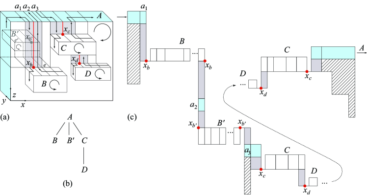
Figure 2: (a) Orthogonal polyhedron. (b) Unfolding tree $T_{U}$. (c) Unfolding of bands and front (hachured) face pieces. Vertex connection through the pivots points $x_{b}$, $x_{b^{\prime}}$, $x_{c}$, $x_{d}$ is shown exaggerated for clarity.

The reason for the $3\times 1$ refinement is that the upper edge $e^{\prime}$ of the back child band $B^{\prime}$ has the same $(x,z)$-coordinates as the upper edge $e$ of $B$ on the front face. In this case, the faces of band $A$ induced by the connecting paths to $B$ would be “overutilized” if there were only two. Let $a_{1},a_{2},a_{3}$ be the three faces of $A$ induced by the $3\times 1$ refinement of the connecting path to $B$, as in Fig. 2. Then the unfolding path winds around $A$ to $a_{1}$, follows the forward connecting path to $B$, returns along the return connecting path to $a_{2}$, crosses over $A$ and unfolds $B^{\prime}$ on the back face, with the return path now joining to $a_{3}$, at which point the unfolding of $A$ resumes. In this case, the pivot point $x_{b^{\prime}}$ for $B^{\prime}$ is the $\frac{2}{3}$-point of $e^{\prime}$. Other such conflicts are resolved similarly. It is now easy to see that the resulted net has the general form illustrated in Fig. 2b:

1. The faces of each band fall within a horizontal rectangle whose height is the band width.

2. These band rectangles are joined by vertical connecting paths on either side, connecting through pivot points.

3. The strip of the plane above and below each band face that is not incident to a connecting path, is empty.

4. The net is therefore an orthogonal polygon monotone with respect to the horizontal.

5.3 Attaching Front and Back Faces to the Net

Finally, we “hang” front and back faces from the bands as follows. The front face of each band $A$ is partitioned by imagining $A$ to illuminate downward lightrays from the rim in the front face. The pieces that are illuminated are then hung vertically downward from the horizontal unfolding of the $A$ band. The portions unilluminated will be attached to the obscuring bands.

In the example in Fig. 2, this illumination model partitions the front face of $A$ into three pieces (the striped pieces in Fig. 2b). These three pieces are attached under $A$; the portions of the front face obscured by $B$ but illuminated downward by $B$ are hung beneath the unfolding of $B$ (not shown in the figure), and so on. Because the vertical illumination model produces vertical strips, and because the strips above and below the band unfoldings are empty, there is always room to hang the partitioned front face. Thus, any orthogonal polygon may be vertex-unfolded with a $3\times 1$ refinement of the vertex grid.

Although we believe this algorithm can be improved to $2\times 1$ refinement, the complications needed to achieve this are similar to what is needed to avoid refinement entirely, so we instead turn directly to $1\times 1$ refinement.

6 $(1\times 1)$-Algorithm

Although the $(1\times 1)$-algorithm follows the same general outline as the $(3\times 1)$-Algorithm, there are significant complications, which we outline before detailing. First, without the refinement of $z$-beams into three strips to allow avoidance of conflicts on opposite sides of a slab (e.g., $B$ and $B^{\prime}$ in Fig. 2a), we found it necessary to replace the $z$-beams by a pair of $z$-rays that are in some sense the boundary edges of a $z$-beam. Selecting two rays per band permits a 2-coloring algorithm (Theorem 3) to identify rays that avoid conflicts. Generating the ray-pairs (Sec. 6.1.1) requires care to ensure that the band graph $G_{b}$ is connected (Sec. 8). This graph, and the 2-coloring, lead to an unfolding tree $T_{U}$ (Sec. 6.2). From here on, there are fewer significant differences compared to the $(3\times 1)$-Algorithm. Without the luxury of refinement, there is more need to share vertical paths on the vertical face of a slab (Fig. 11). Finally, the vertical connecting paths obscure the illumination of some grid faces, which must be attached to the connecting paths. We now present the details, in this order:

 

1. Select Pivot Points (Sec. 6.1) via
	a. Ray-Pair Generation (Sec. 6.1.1)
	b. Ray Graph (Sec. 6.1.2)
2. Construct $T_{U}$ (Sec. 6.2)
3. Select Connecting Paths (Sec. 6.2.1)
4. Determine Unfolding Directions (Sec. 6.2.2)
5. Recurse:
	a. Unfold Bands into a Net (Sec. 6.3)
	b. Attach Front and Back Faces to the Net (Sec. 6.4)

 

6.1 Selecting Pivot Points

The pivot $x_{a}$ for a band $A$ is the gridpoint of $A$ where the unfolding of $A$ starts and ends. The $y$-edge of $A$ incident to $x_{a}$ is the first edge of $A$ that is cut to unfold $A$.

Let $A$ be an arbitrary band delimited by planes $Y_{i}$ and $Y_{i+1}$. Say that two gridpoints $u\in Y_{i}$ and $w\in Y_{i+1}$ are in conflict if the upward rays emerging from $u$ and $w$ hit the endpoints of the same $y$-edge of $A$; otherwise, $u$ and $v$ are conflict-free. If $u$ lies either on a vertical edge, or on a vertically extreme horizontal edge, then the ray at $u$ degenerates to $u$ itself.

Our goal is to select conflict-free pivots for all bands in $T_{U}$, which will help us avoid later competition over the use of certain faces in the unfolding, an issue that will become clear in Sec. 6.3. Selecting these pivots is the most delicate aspect of the $(1\times 1)$-algorithm. Ultimately, we represent pivoting conflicts in the form of a graph $G_{r}$ (Sec. 6.1.2), from which $T_{U}$ will be derived.

6.1.1 Ray-Pair Generation

In order to avoid pivoting conflicts, for each band we will need two choices for its connecting ray. Thus the algorithm generates the rays in pairs. Because there is no refinement, the two rays originate at grid points on the same band, but they may terminate on different bands. A simple example is shown in Figure 3a, where the ray pair originating on band $D$ hits two different bands, $B$ and $C$. This example also suggests that one cannot consider ray pairs connecting pairs of bands, as in the $(3\times 1)$-algorithm (which would connect $D$ to $A$ in this example), but instead we focus on shooting pairs of rays upward from strategic locations on the boundary of each band, and then selecting a subset of these rays so that the conflicts can be resolved and $T_{U}$ is connected. To ensure connectedness of all bands, several ray-pairs must be issued upward from each band. Figure 3b shows an example: no pair of rays can emanate upward from the top of $B\cap P^{-}$ or $C\cap P^{-}$; one pair of rays shoots upward from the top of each component of $A\cap P^{-}$: $(r_{1},r_{2})$ connects $A$ to $B$ and $(r_{3},r_{4})$ connects $A$ to $C$; finally, one pair of rays $(r_{5},r_{6})$ issues from the top of $A\cap P^{-}$, which connects $A$ to $D$. So, overall, three pairs of rays are generated for band $A$. We now turn to describing in detail the method for generating ray-pairs.

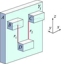
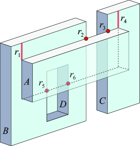
(a)	(b)

Figure 3: (a) The ray pair $(r_{1},r_{2})$ connects band $D$ to two different bands $B$ and $C$. (b) To ensure connectivity, three pairs of rays must be issued for $A$: $(r_{1},r_{2})$, $(r_{3},r_{4})$ and $(r_{5},r_{6})$.

Let band $A$ intersect plane $Y_{i}$. The algorithm is a for-loop over all $A$. Let $A_{1},A_{2},\ldots,A_{m}$ be the components of $A$, defined as follows. Take all the maximal components of $A\cap P^{+}$ that contain an $x$-gridedge, and union with all the maximal components of $A\cap P^{-}$ that contain an $x$-gridedge. We define $S(A_{j})$ as the set of all potential rays shooting upward from $A_{j}$. More precisely, $S(A_{j})$ consists of the set of all segments $s=(a,b)$, with $a\in A_{j}$, such that

1. Either $s$ is a point, with $b=a$, or $s\subset P\subset Y_{i}$ is vertical (parallel to $z$), with $a$ below $b$.

2. $b\in B$ for some band $B\neq A$.

3. The open segment $s\setminus\{a,b\}$ may contain points of $A$ (see $r_{2}$ in Fig. 4b), but no other band points.

For each band $A$, for each component $A_{j}\subseteq A$, if $S(A_{j})$ is nonempty, we select one ray pair $(r_{1},r_{2})$, such that (i) $r_{1}$ is the leftmost segment in $S(A_{j})$ that is incident to a highest $x$-gridedge in $A_{j}$, and (ii) $r_{2}$ is the segment one $x$-gridedge to the right of $r_{1}$. Fig. 4 shows a few examples.

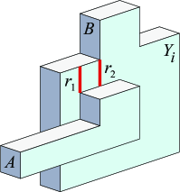
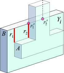
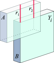
(a)	(b)	(c)

Figure 4: Generating ray-pairs: (a) $(r_{1},r_{2})$ for $A$; $S(B)=\emptyset$. (b) $(r_{1},r_{2})$ for $A$ (note that $r_{2}$ runs along source band $A$); degenerate ray-pair $(r^{\prime}_{1},r^{\prime}_{2})$ for $B$. (c) $S(A)=\emptyset$; $(r_{1},r_{2})$ for $B$.

As mentioned above, several ray pairs could be generated for any one band, and indeed several pairs connecting two bands.

Let $G_{b}$ be the band graph whose nodes are bands. Two bands are connected by an arc in $G_{b}$ if the ray-pair algorithm generates a ray connecting them. We call a collection of bands in $G_{b}$ ray-connected if they are in the same connected component of $G_{b}$. We establish that $G_{b}$ is a connected graph, i.e., all bands are ray-connected to one another, even if only one ray per pair is employed:

Lemma 1

$G_{b}$ is connected. Furthermore, the subgraph of $G_{b}$ induced by exactly one ray per ray-pair (arbitrarily selected) is connected.

Whereas the connectedness of bands by $z$-beams in the $(3\times 1)$-algorithm is straightforward, the complex possible relationships between bands makes connectedness via rays more subtle. We relegate the proof to the Appendix (Sec. 8) in order to not interrupt the main flow of the algorithm.

The over-generation of ray-pairs noted above is designed to ensure connectedness. Eventually many rays will be discarded by the time $T_{U}$ is constructed in Sec. 6.2.

6.1.2 Ray Graph $G_{r}$

One pair of rays per pair of bands suffices to ensure that all bands are ray-connected. If multiple pairs of rays exist for a pair of bands, pick one pair arbitrarily and discard the rest. Then define a ray graph $G_{r}$ as follows. The nodes of $G_{r}$ are vertical rays in a plane $Y_{i}$, perhaps degenerating to points, connecting gridpoints between two bands that both intersect $Y_{i}$. The arcs of $G_{r}$ each records a potential pivoting conflict, and are of two varieties:

1. The nodes for the two rays issuing from the top of one band $B$ are adjacent in $G_{r}$. Call such arcs $x$-arcs; geometrically they can be viewed as parallel to the $x$-axis.

2. The nodes for two rays incident to opposite sides of the rim of a band $A$, connected by a $y$-segment on the band, are adjacent in $G_{r}$. Call such arcs $y$-arcs; geometrically they can be viewed as parallel to the $y$-axis.

Fig. 5 shows two simple examples of $G_{r}$ involving nodes on opposite sides of one band $A$.

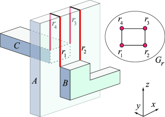
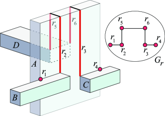
(a)	(b)

Figure 5: Building $G_{r}$. (a) $G_{r}$ is a $4$-cycle; $\{r_{1},r_{2}\}$ and $\{r_{3},r_{4}\}$ are $x$-arcs; any other arc is a $y$-arc. (b) $G_{r}$ is a path; $\{r_{2},r_{5}\}$ and $\{r_{3},r_{6}\}$ are $y$-arcs; any other arc is an $x$-arc.

Before proceeding, we list the consequences of the two types of arcs in $G_{r}$. Assuming that we can $2$-color $G_{r}$ $\{$red, blue$\}$, and we select the base of (say) the red rays as pivots, then: (i) exactly one pivot is selected for each band, and (ii) no two pivot rays are in conflict across a band. So our goal now is to show that $G_{r}$ is $2$-colorable. Because a graph is $2$-colorable if and only if it is bipartite, and a graph is bipartite if and only if every cycle is of even length, we aim to prove that every cycle in $G_{r}$ is of even length. We start by listing a few relevant properties of $G_{r}$:

1. Every node $r\in G_{r}$ has exactly one incident $x$-arc. The rays are generated in pairs, and the pairs are connected by an $x$-arc. As no such ray is shared between two bands, at most one $x$-arc is incident to any $r$.

2. Nodes have at most degree $3$, with the following structure: degree-$1$ nodes have an incident $x$-arc; degree-$2$ nodes have both an incident $x$- and $y$-arc; and degree-$3$ nodes have an incident $x$-arc and two incident $y$-arcs.

3. Each $x$-arc spans exactly one pair of adjacent $y$-gridlines, and each $y$-arc spans exactly one band rim-to-rim. The former is by the definition of ray pairs, which issue from adjacent gridpoints, and the latter follows from the grid partitioning of the object into bands.

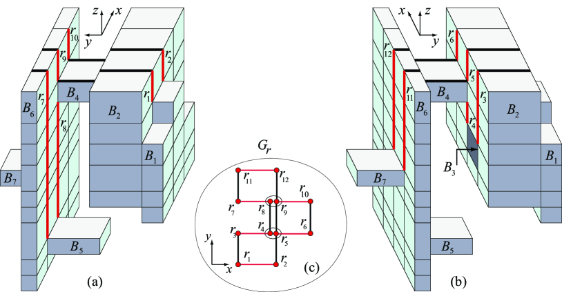
Figure 6: (a,b) Two side views of an object; $z$-rays and $y$-arcs are marked with thick lines. (c) $G_{r}$ coordinatized into $xy$-plane $\Pi$; $(r_{5},r_{6},r_{10},r_{9})$ is a $4$-cycle; $(r_{1},r_{3},r_{4},r_{8},r_{7},r_{11},r_{12},r_{9},r_{5},r_{2})$ is a $10$-cycle.

Our next step requires embedding $G_{r}$ in an $xy$-plane $\Pi$. Toward that end, we coordinatize the nodes and arcs of $G_{r}$ as follows. A node $r\in G_{r}$ is a $z$-ray, and is assigned the $(x,y)$ coordinates of the ray. Note that this means collinear rays get mapped to the same point; however we treat them as distinct. The $x$-arcs are then parallel to the $x$-axis, and the $y$-arcs are parallel to the $y$-axis. In essence, this coordinatization is a view from $z=+\infty$.

Fig. 6 shows a more complex example illustrating this viewpoint. The object is composed of $7$ bands $B_{i}$, one of which ($B_{3}$) is a dent. There are $12$ ray nodes, two pairs of which lie on the same $z$-vertical line, namely $(r_{4},r_{5})$ and $(r_{8},r_{9})$. Note that there are $y$-arcs crossing both the top of and the bottom of $B_{4}$. The graph $G_{r}$ has a $4$-cycle and a $10$-cycle, both detailed in the caption (as well as a $12$-cycle not detailed).

Lemma 2

Every cycle in $G_{r}$ is of even length.

Proof: Let $C$ be a cycle in $G_{r}$. The coordinatization described above maps $C$ to a (perhaps self-crossing) closed path in the $xy$-plane $\Pi$, a path which may visit the same $(x,y)$ point more than once, and/or traverse the same edge in $\Pi$ more than once. Any such closed path on a grid must have even length, for the following reason.

First, by Property (3) above, each edge of the path in $\Pi$ connects adjacent grid lines: an edge never “jumps over” one or more grid lines. Second, any such closed lattice path changes parity with each step, in the following sense. Number the $x$- and $y$-gridlines with integers $0,1,2,\ldots$ left to right and bottom to top respectively. Define the parity of a gridpoint of $\Pi$ to be the sum of its $x$- and $y$-gridline coordinates, mod $2$. Then each step of the path, necessarily in one of the four compass directions, changes parity, as it changes only one of $x$ or $y$. Returning to the start point to close the path must return to the starting coordinates, and so to the same parity. Thus, there must be an even number of parity changes along any closed path. Therefore, $C$ has an even number of edges.  

We have now established this:

Theorem 3

$G_{r}$ is $2$-colorable.

Note that nowhere in the above proof do we assume genus zero, so this theorem holds for polyhedra of arbitrary genus.

Band pivoting.

By Theorem 3, we can $2$-color the nodes of $G_{r}$ {red,blue}. We choose all red ray-nodes of $G_{r}$ to be pivoting rays, in that their base points become pivot points. As remarked before, this selection guarantees that each band is pivoted, and no two pivots are in conflict.

6.2 Unfolding Tree $T_{U}$

The next task is to define a band spanning tree $T_{U}$, based on the band graph $G_{b}$. Define $G^{\prime}_{b}$, to retain the just the arcs of $G_{b}$ corresponding to the red ray nodes (in the above $2$-coloring) in $G_{r}$. This maintains the connectivity of Lemma 1. Then take $T_{U}$ to be any spanning tree of $G^{\prime}_{b}$ rooted at a frontmost band.

With $T_{U}$ finally in hand, the remainder of the $(1\times 1)$-algorithm follows the overall structure of the $3\times 1$ algorithm, with variations as mentioned before, as detailed below.

6.2.1 Selecting Connecting Paths

Having established a pivot point for each band, we are now ready to define the forward and return connecting paths for a child band in $T_{U}$. Let $B$ be an arbitrary child of a band $A$. If $B$ intersects $A$, both forward and return connection paths for $B$ reduce to the pivot point $x_{b}$ (e.g., $u$ in Fig. 7). If $B$ does not intersect $A$, then a ray $r$ connects $x_{b}$ to $A$ (Figs. 8a and 10a). The connecting paths are the two vertical paths separated by $r$ comprised of the gridfaces sharing an edge with $r$ (paths $a_{1}$ and $a_{2}$ in Figs. 8a and 10a). The path first encountered in the unfolding of $A$ is used as a forward connecting path; the other path is used as a return connecting path.

6.2.2 Determining Unfolding Directions

A top-down traversal of $T_{U}$ assigns an unfolding direction to each band in $T_{U}$ as follows. The root band in $T_{U}$ may unfold either cw or ccw, but for definiteness we set the unfolding direction to cw. Let $B$ be the band in $T_{U}$ currently visited and let $A$ be the parent of $B$. If the upward ray $r$ incident to $x_{b}$ connects $B$ to a bottom gridpoint of $A$, and if $A$ unfolds cw(ccw), then $B$ unfolds cw(ccw). Otherwise, $r$ connects $B$ to a top or a side (for degenerate rays) gridpoint of $A$; in this case, if $A$ unfolds cw(ccw), then $B$ unfolds ccw(cw). In other words, $A$ and $B$ unfold in a same direction if $B$ “hangs below” $A$, and in opposite direction otherwise.

6.3 Unfolding Bands into a Net

Let $A$ be a band to unfold, initially the root band. The unfolding of $A$ starts at $x_{a}$ and proceeds in the unfolding direction (cw or ccw) of $A$. Henceforth we assume w.l.o.g. that the unfolding of $A$ proceeds cw (w.r.t. a viewpoint at $y=-\infty$); the ccw unfolding of $A$ is a vertical reflection of the cw unfolding of $A$. In the following we describe our method to unfold every child $B$ of $A$ recursively, which falls naturally into several cases.

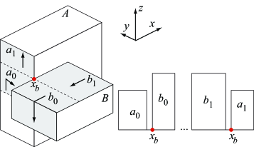
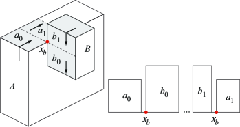
Figure 7: Unfolding $B$ when the ray connecting $B$ to $A$ degenerates to $x_{b}$.

Case 1:

Pivot $x_{b}\in A\cap B$. Then, whenever the unfolding of $A$ reaches $x_{b}$, we unfold $B$ as in Fig. 7. The unfolding uses the two band faces of $A$ incident to $x_{b}$ ($a_{0}$ and $a_{1}$ in Fig. 7). The gridface $b_{0}$ of $B$ ccw of $x_{b}$ gets rotated around $x_{b}$ so that the ccw unfolding of $B$ extends horizontally to the right. The unfolding of $B$ proceeds ccw back to $x_{b}$, then the face $a_{1}$ incident to $x_{b}$ gets oriented about $x_{b}$ so that the unfolding of $A$ continues horizontal to the right.

Note that, because the pivots of any two children of $A$ are conflict-free, there is no competition over the use of $a_{0}$ and $a_{1}$ in the unfolding. Note also that the unfolding path does not self-cross. For example, the cyclic order of the faces incident to $u$ in Fig. 7a is $(a_{0},A_{front},b_{0},b_{1},B_{back},a_{1})$, and the unfolding path follows $(a_{0},b_{0},\ldots,b_{1},a_{1})$.

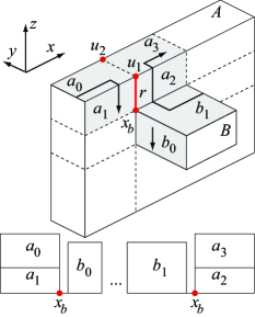
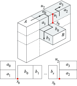
(a)	(b)

Figure 8: Unfolding $B$: $u_{1}$ is not a corner vertex of $A$ (a) $x_{b}$ incident to a left face of $B$ (b) $x_{b}$ incident to a top face of $b$.

Case 2:

Pivot $x_{b}\not\in A\cap B$ and the (forward, return) connecting paths for $B$ do not overlap other connecting paths (except at their boundaries); we will later see that this may happen. Let us settle some notation first (cf. Fig 8a): $r$ is the ray connecting $B$ to $A$; $a_{1}$ and $a_{2}$ are forward and return connecting paths for $B$ (one to either side of $r$); $u_{1}$ is the endpoint of $r$ that lies on $A$; and $u_{2}$ is the other endpoint of the $y$-edge of $A$ incident to $u_{1}$. We discuss three situations:

Case 2a:

$u_{1}$ is neither a reflex corner nor a bottom corner of $A$. In this case, whenever the unfolding of $A$ reaches $a_{1}$, the unfolding of $B$ proceeds as in Fig. 8a or Fig. 8b, depending on whether $x_{b}$ touches a left face of $B$ or not. In either case, if $b_{0}$ is the face of $B$ extending ccw left of $x_{b}$, rotate $b_{0}$ so that the unfolding of $B$ extends horizontal to the right, recursively unfold $B$, then rotate the return path $a_{2}$ about $x_{b}$ so that the unfolding of $A$ continues horizontal to the right.

Case 2b:

$u_{1}$ is a reflex corner of $A$. In this case, the unfolding of $B$ proceeds as in Fig. 9(a, b). It is the existence of the vertical strip incident to $u_{1}$ (marked $t$ in Fig. 9) that makes handling this case different from Case 2a above. Note however that the existence of $t$ implies the existence of at least two gridfaces on either the return path or the forward path for $B$, depending on whether $t$ is a left (Fig. 9a) or a right (Fig. 9b) strip of faces. In the former case the unfolding starts as in Case 2a (Fig. 9a), and once the unfolding of $B$ returns to $x_{b}$, it continues along the return path up to $u_{1}$, then unfolds $t$ and orients it about $u_{1}$ in such a way that the unfolding of $A$ continues horizontal to the right. The portion of the return path that extends above $u_{1}$ ($a_{20}$ in Fig. 9a) gets attached below the adjacent top face of $A$ ($a_{3}$ in Fig. 9a).

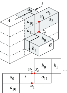
(a)	(b)

Figure 9: Unfolding $B$: $u_{1}$ is a corner vertex of $A$. (a) $t$ is a left strip (b) $t$ is a right strip.

If $t$ is a strip of right faces, then $t$ gets unfolded before descending along the forward path down to $B$, as in Fig. 9b (note the vertical symmetry with the unfolding in Fig. 9a); the unfolding of $B$ then proceeds as in Case 2a (Fig. 8b).

Case 2c:

$u_{1}$ is a bottom corner of $A$. In this case, the unfolding proceeds as in Fig. 10a or Fig. 10b, depending on whether $u_{1}$ is a right or a left bottom corner of $A$. The unfolding illustrated in Fig. 10a follows the familiar unfolding pattern: orient the face of $B$ ccw left of $x_{b}$ so that the unfolding of $B$ extends to the right; once the unfolding of $B$ returns to $x_{b}$, follow the return path back to $A$ and unfold the face of $A$ cw to the right of $u_{1}$ ($a_{3}$ in Fig. 10a) so that the unfolding of $A$ continues horizontal to the right.

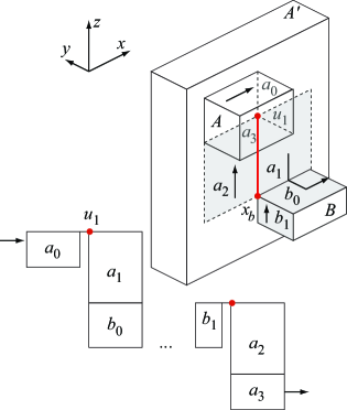
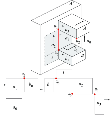
(a)	(b)

Figure 10: Unfolding $B$: $u_{1}$ is a bottom corner of $A$ (a) rightmost, and (b) leftmost face of $A$ vertically aligned with leftmost face of $B$.

A similar pattern applies to the case illustrated in Fig. 10b, with one subtle difference meant to aid in unfolding front and back faces (discussed in Sec. 6.4): in unfolding bands, we aim at maintaining the vertical position of the (forward, return) connecting paths in the unfolding, so that vertical strips hanging below these connecting paths could also hang vertically in the unfolding. More on this in Sec. 6.4. Observe that $a_{1}$ and $a_{2}$ from Fig. 10a hang downward in the unfolding. However, if $a_{2}$ were to maintain its vertical position in the unfolding from Fig. 10b, it would not be possible to orient $a_{3}$ around $u_{1}$ so as to continue unfolding $A$ horizontal to the right of $a_{2}$. This is the reason for employing the face marked $t$ in the unfolding, so that vertical sides of $t$ remain vertical in the unfolding, and any face strip hanging below $t$ could be attached to $t$ vertically in the unfolding.

We note that Fig. 10 illustrates only the situation in which $x_{b}$ is incident to a left face of $B$, but it should not be difficult to observe that an exact same idea applies to any top pivot of $B$; the pivot position only affects the start and end unfolding position of $B$, and everything else remains the same.

Case 3:

Pivot $x_{b}\not\in A\cap B$ and a connecting path for $B$ overlaps a connecting path for another descendant $C$ of $A$. This case is slightly more complex, because it involves conflicts over the use of the connecting paths for $B$. The following three situations are possible.

Case 3a:

The forward path $a_{1}$ for $B$ overlaps the return path for another descendant $C$ of $A$. This situation is illustrated in Fig. 11a. In this case, the unfolding $B$ starts as soon as the unfolding along the return path from $C$ to $A$ meets a face of $B$ incident to $x_{b}$ (face $b_{0}$ in Fig. 11a). At this point $B$ gets recursively unfolded as before (see Fig. 11b), then the unfolding continues along the return path for $C$ back to $A$. Fig. 11b shows face $a_{1}$ in two positions: we let $a_{1}$ hang down only if the next face to unfold is a right face of a child of $A$ (see the transition from $k_{7}$ to $c_{5}$ in Fig. 12); otherwise, use $a_{1}$ in the upward position, a freedom permitted to us by rotating about vertex $u$.

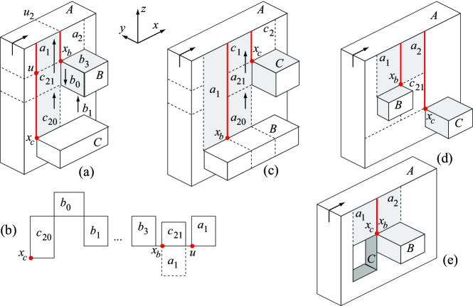
Figure 11: (a) Return path for $C$ includes $c_{20},c_{21},a_{1}$; forward path for $B$ is $a_{1}$. (b) Unfolding for (a) (c) Return path for $B$ includes $a_{20},a_{21},c_{1}$; forward path for $C$ is $c_{1}$. (d) Return path for $B$ is $a_{2}$; forward path for $C$ includes $a_{2},c_{21}$. (e) Forward (return) paths are identical for $B$ and $C$.

Case 3b:

The return path $a_{2}$ for $B$ overlaps the forward path for another descendant $C$ of $A$. This situation is illustrated in Figs. 11c and 11d. The case depicted in Fig. 11c is similar to the one in Fig. 11a and is handled in the same manner. For the case depicted in Fig. 11d, notice that $a_{2}$ is on both the forward path for $C$ and the return path for $B$. However, no conflict occurs here: from $a_{2}$ the unfolding continues downward along the forward path to $C$ and unfolds $C$ next.

Case 3c:

The forward path $a_{1}$ for $B$ overlaps the forward path for another descendant $C$ of $A$. This situation occurs when either $B$ or another band $C$ incident to $B$ is a dent, as illustrated in Figs. 11e. Again, no conflict occurs here: the recursive unfolding of $C$, which returns to $x_{c}=x_{b}$, is followed by the recursive unfolding of $B$, which returns to $x_{b}$, then the unfolding continues along the return path for $B$ ($C$) back to $A$.

Fig. 12 shows a more complex example that emphasizes these subtle unfolding issues. Note that the return path $k_{1},k_{8},k_{9}$ for $B$ overlaps the forward path $k_{9}$ for $C$; and the return path $k_{5},k_{6}$ and $k_{7}$ for $G$ overlaps the forward path for $H$, which includes $k_{7}$. The unfolding produced by the method described in this section is depicted in Fig. 12(b).

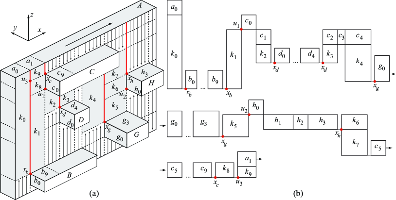
Figure 12: (a) An example. (b) The vertex-unfolding.

6.4 Attaching Front and Back Faces to the Net

Front and back faces of a slab are “hung” from bands following the basic idea of the illumination model discussed in Sec. 5.3. There are three differences, however, caused by the employment of some front and back gridfaces for the connecting paths, which can block illumination from the bands.

1. We illuminate both upward and downward from each band: each $x$-edge illuminates the vertical face it attaches to. This alone already suffices to handle the example in Fig. 12: all vertical faces are illuminated downward from the top of $A$, upward from the bottom of $A$, and upward from the top of $B$.

2. Some gridfaces still might not be illuminated by any bands, because they are obscured both above and below by paths in connecting faces. Therefore we incorporate the connecting faces into the band for the purposes of illumination. For example, in Fig. 10a, $a_{2}$ illuminates downward and $a_{1}$ illuminates upward. The reason this works is that, with one exception, each vertical connecting strip remains vertical in the unfolding, and so illuminated strips can be hung safely without overlap.

3. The one exception is the forward connecting path $a_{1}$ in Fig. 10b. This paths unfolds “on its side,” i.e., what is vertical in 3D becomes horizontal in 2D. Note, however, that the face $x$ below each of these paths (a face always present), is oriented vertically. We thus consider $x$ to be part of the connecting path for illumination purposes, permitting the strip below to be hung under $x$.

Because our cases are exhaustive, one can see now that all gridfaces of (say) the front face of $A$ are either illuminated by $A$, or by some descendant of $A$ on the front face, augmented by the connecting paths as just described. (In fact every gridface is illuminated twice, from above and below.) Hanging the strips then completes the unfolding.

6.5 Algorithm Complexity

Because there are so few unfolding algorithms, that there is some algorithm for a class of objects is more important than the speed of the algorithm. Nevertheless, we offer an analysis of the complexity of our algorithm. Let $n$ be the number of corner vertices of the polyhedron, and $N=O(n^{2})$ the number of gridpoints. The vertex grid can be easily constructed in $O(N)$ time, leaving a planar surface map consisting of $O(N)$ gridpoints, gridedges, and gridfaces. The computation of connecting rays (Sec. 6.2) requires determining the components of $A\cap P^{+}$ and $A\cap P-$, for each $A$. This can be easily read of from the planar map by running through the $n$ vertices of each of the $O(n)$ bands and determining, for each vertex, whether it belongs to $P^{+}$ or $P^{-}$. Each of the $O(n)$ band components shoots a vertical ray from one corner vertex, in a 2D environment (the plane $Y_{i}$) of $n$ noncrossing orthogonal segments. Determining which band a ray hits involves a ray shooting query. Although an implementation would employ an efficient data structure, perhaps BSP trees [PY92], for complexity purposes the naive $O(n)$ query cost suffices to lead to $O(n^{2})$ time to construct $G_{r}$. Selecting pivots (Sec. 6.1) involves 2-coloring $G_{r}$ in $O(n)$ time, and computing the unfolding tree $T_{U}$ in a breadth-first traversal of $G_{r}$, which takes $O(n)$ time. Unfolding bands (Sec. 6.3) involves a depth-first traversal of $T_{U}$ in $O(n)$ time, and laying out the $O(N)$ gridfaces in $O(N)$ time. Thus, the algorithm can be implemented to run in $O(N)=O(n^{2})$ time.

7 Further Work

Extending these algorithms to arbitrary genus orthogonal polyhedra remains an interesting open problem. Holes that extend only in the $x$ and $z$ directions within a slab seem unproblematic, as they simply disconnect the slab into several components. Holes that penetrate several slabs (i.e, extend in the $y$ direction) present new challenges. One idea to handle such holes is to place a virtual $xz$-face midway through the hole, and treat each half-hole as a dent (protrusion).

Acknowledgements

We thank the anonymous referees on [DFO06] for their careful reading and insightful comments.

8 Appendix: Proof of Lemma 1 (Connectedness of $G_{b}$)

Two subsets of $P\subset Y_{i}$ are path-connected, or just connected, if there are points in each that are connected by a path that lies in $P$. We need some notation to describe the portions of $r(A)$ that are relevantly connected to each band $A$. For a protrusion $A$, let $r_{c}(A)$ be the subset of $r(A)$ (cf. Sec. 2) that is path-connected to $A$ via paths that do not cross any bands. For a dent $B$, let $r_{c}(B)$ be the boundary of $B$ plus the subset of $r(B)$ that is both path-connected to $B$ via paths that do not cross any bands, and is not part of $r_{c}(A)$, for some protrusion $A$. Consider for example Figure 14b. For protrusion $B^{\prime}$, $r_{c}(B^{\prime})$ consists of the boundary rim of $B^{\prime}$ and the portion of the back face of $B^{\prime}$ that overhangs dent $B$. For dent $B$, $r_{c}(B)$ consists only the boundary of $B$, even though the overhanging portion of $B^{\prime}$ can be reached from $B$ without crossing any bands, because that is part of $r_{c}(B^{\prime})$. In Figure 16a however, the portion of the front face of $A^{\prime}$ enclosed by $B$ belongs to $r_{c}(B)$, not to $r_{c}(A^{\prime})$.

The genus-zero assumption implies that, for protrusion $A$ and dent $B$ on opposite sides of $Y_{i}$ such that $r_{c}(A)\cap r_{c}(B)$ is nonempty, it must be that $A\cap B$ is nonempty (cf. Figs. 15). Define

$$r_{c}(A,B)=\left\{\begin{tabular}[]{ll}$A\cap B$,&if $A\cap B\neq\emptyset$, and at least one of $A$ and $B$ is a dent\\ $r_{c}(A)\cap r_{c}(B)$&otherwise.\end{tabular}\right.$$

This definition is intended to identify gridpoints on either $A$ or $B$ from which rays are issued by the ray-pair generation algorithm (Sec. 6.1.1). The reason for treating intersecting dents and protrusions differently is a subtle one, and is captured by Fig. 14b: $B$ is a dent behind $Y_{i}$ and $B^{\prime}$ is a protrusion in front of $Y_{i}$; $r_{c}(B^{\prime})$ is the piece of the back face of $B^{\prime}$ enclosed by $B$; $u$ is a highest gridpoint in $B\cap B^{\prime}$, while $w$ is a highest gridpoint in $r_{c}(B)\cap r_{c}(B^{\prime})$; $u$ is a potential ray basepoint, while $w$ is not. The above definition eliminates points such as $w$ from the set $r_{c}(A,B)$.

Our connectivity proof for $G_{b}$ proceeds as follows. In general, there are a number of disconnected maximal components $P_{1},P_{2},\ldots$ of $P$, with $P=P_{1}\cup P_{2}\cup\cdots$. The bands incident to each of these are ray-connected to each other via planes other than $Y_{i}$. We first argue that, to prove that $G_{b}$ is ray-connected, it suffices to prove that each $P_{j}$ is ray-connected. Remove from $O$ all the slabs $S_{1},S_{2},\ldots$ incident to $Y_{0}$. Establish that the bands in the resulting object $O^{\prime}$ are ray-connected, via induction. Now put back the slabs. Each $S_{j}$ corresponds to a component $P_{j}$, and we are assuming we can establish that all bands incident to $P_{j}$ are ray-connected to one another. This along with the fact that $O$ itself is connected implies that all bands are ray-connected. Henceforth we concentrate on one such connected component $P_{j}$, call it $Q\subset Y_{i}$ for succinctness. Let ${\cal C}$ be the collection of all bands that intersect $Q$. Then $\displaystyle\cup_{A\in{\cal C}}r_{c}(A)=Q$. The idea of the connectedness proof is that the bands get connected in upward chains, and ultimately to each other through “common ancestor” higher bands. We choose to prove it by contradiction, arguing that a highest disconnected component cannot exist.

Lemma 4

All bands in ${\cal C}$ are ray-connected. Furthermore, if one arbitrary ray in each ray-pair is discarded, $C$ remains ray-connected.

Proof: For the purpose of contradiction, assume that not all bands in ${\cal C}$ are ray-connected. Let ${\cal C}_{1},{\cal C}_{2},\ldots$ be the distinct maximal subsets of ${\cal C}$ that are ray-connected. Let $Q_{j}=\cup_{A\in{\cal C}_{j}}r_{c}(A)$. Then $Q=\cup_{j}Q_{j}$. Since $Q$ is connected, the subsets $Q_{j}$ are not disjoint, in that for every $Q_{j}$ there is an $Q_{k}$ such that $Q_{j}\cap Q_{k}$ is nonempty. By the observation above, this means that

$$Q_{jk}=\cup_{A\in{\cal C}_{j},B\in C_{k}}~{}r_{c}(A,B)$$

is also nonempty. Let $j$ and $k$ be such that $Q_{jk}$ contains a highest $x$-gridedge (gridpoint, if $Q_{jk}$ contains only isolated points) among all $Q_{jk}$. Let $u$ be the leftmost highest gridpoint in $Q_{jk}$. Let $A\in{\cal C}_{j}$ and $B\in{\cal C}_{k}$ be such that $u\in r_{c}(A,B)$.

We have thus identified two bands $A$ and $B$, ray-disconnected because in different components of $Q$, which contribute this highest gridpoint $u$ in the “highest” intersection $Q_{jk}$. We now examine in turn the four protrusion/dent possibilities for these two bands.

Case 1. $A$ and $B$ are both protrusions on opposite sides of $Y_{i}$. Assume w.l.o.g that $A$ is behind $Y_{i}$, $B$ is in front of $Y_{i}$, and $u$ is on $B$ (as depicted in Fig. 13).

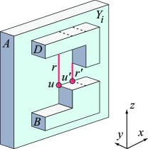
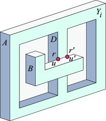
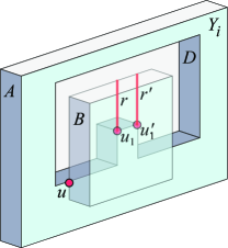
(a)	(b)

Figure 13: Case 1: $A$ and $B$ are both protrusions on opposite sides of $Y_{i}$ (a) $D$ is a protrusion (b) $D$ is a dent with a vertical side incident to $u$ (c) $D$ is a dent with a bottom edge incident to $u$.

We discuss two subcases:

1. $u$ is on a top edge of $B$ (Figs. 13(a,b)). Then our ray-pair algorithm generates a ray-pair $(r,r^{\prime})$, with $r$ incident to $u$ and $r^{\prime}$ incident to the gridpoint $u^{\prime}$ cw from $u$. Consider $r$ (the analysis is similar for $r^{\prime}$). If $r$ hits $A$, then in fact $A$ and $B$ are ray-connected, contradicting the fact that $A$ and $B$ belong to different ray-connected components of ${\cal C}$. So let us assume that $r$ hits another band $D\in C_{\ell}$. Fig. 13a(b) illustrates the situation when $D$ is a protrusion (dent). If $D\in{\cal C}_{j}$, then $D$ and $A$ are ray-connected in $C_{j}$, and since $B$ and $D$ are ray-connected, it follows that $B$ and $A$ are ray-connected, a contradiction. So assume that $D\in{\cal C}_{\ell}$, with $\ell\neq j$. But then $r_{c}(A,D)$ (and implicitly $Q_{j\ell}$) has a gridpoint higher than $u$, contradicting our choice of $j$, $k$ and $u$.

2. $u$ is on a vertical (left, right) edge of $B$ (Fig. 13c). Then $u$ must be at the intersection between a dent $D$ and $B$, meaning that $D\cap r_{c}(B)$ is nonempty. Furthermore, $r_{c}(A,D)$ has a gridpoint higher than $u$, meaning that $D\in G_{j}$. Let $u_{1}$ be the leftmost among the highest gridpoints of $D\cap r_{c}(B)$. Then our ray-pair algorithm generates a ray-pair $(r,r^{\prime})$ from $u_{1}$ and its right neighbor $u^{\prime}_{1}$. Consider $r$ (the analysis is similar for $r^{\prime}$). If $r$ hits $B$, then $B$ is ray-connected to $D$, which is ray-connected to $A$, a contradiction. If $r$ hits a band $E$ other than $D$, then it must be that $D\in C_{k}$, since $r_{c}(B,E)$ has a gridpoint higher than $u_{1}$, which is no lower than $u$. This means that $B$ is ray-connected to $E$, which is ray-connected to $D$, which is ray-connected to $A$, a contradiction.

Case 2. $A$ is a protrusion and $B$ is a dent, both on a same side of $Y_{i}$. The case when $A$ and $B$ are both in front of $Y_{i}$ (illustrated in Fig. 14a) is identical to Case 1 above, once one conceptually pops out $B$ into a protrusion. We now discuss the case when $A$ and $B$ are both behind $Y_{i}$.

Assume first that $r_{c}(A,B)$ contains no top edges of $B$, as depicted in Figure 14b. Let $B^{\prime}$ be a protrusion in front of $Y_{i}$ covering the top of $B$. Then $r_{c}(A,B^{\prime})$ and $r_{c}(B^{\prime},B)$ each contains a gridpoint higher than $u$. The following two contradictory observations settle this case:

1. It must be that $B^{\prime}\not\in{\cal C}_{k}$; otherwise $Q_{jk}$ would contain a gridpoint in $r_{c}(A,B^{\prime})$ higher than $u$.

2. If $B^{\prime}\in C_{\ell}$, then it must be that $\ell=k$; otherwise $Q_{\ell k}$ would contain a gridpoint in $r_{c}(B^{\prime},B)$ higher than $u$.

If $r_{c}(A,B)$ contains at least one top gridedge of $B$, then arguments similar to the ones used for the case illustrated in Fig. 13a (conceptually popping $B$ to become a protrusion) settle this case as well.

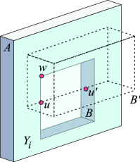
(a)	(b)

Figure 14: Case 2: $A$ is a protrusion and $B$ is a dent (a) behind $Y_{i}$ (b) in front of $Y_{i}$.

Case 3. $A$ is a protrusion and $B$ is a dent on opposite sides of $Y_{i}$ (see Fig. 15). Let $B^{\prime}$ be the protrusion in front of $Y_{i}$ enclosing $B$. We discuss two subcases:

1. $r_{c}(A)$ contains a top edge of $B$ (see Fig. 15a). This means that $r_{c}(A)\cap r(B)$ is nonempty, and the ray-pair algorithm shoots a ray-pair $(r,r^{\prime})$ upward from the endpoints of a highest gridedge $\{u_{1},u^{\prime}_{1}\}$ of $A\cap r(B)$. Consider ray $r$ (the analysis is similar for $r^{\prime})$. If $r$ hits $B$, then $A$ and $B$ are in fact ray-connected, a contradiction. If $r$ hits a band $D$ other than $B$, then arguments similar to the ones for the case illustrated in Fig. 13a (Case 1) lead to a contradiction.

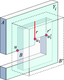
   (a)	(b)

   Figure 15: Case 3: $A$ is a protrusion behind $Y_{i}$; $B$ is a dent in $B^{\prime}$, both in front of $Y_{i}$.

2. $r_{c}(A)$ contains a bottom edge of $B$. This case is symmetrical to the one above in that a ray upward from a gridpoint of $B\cap r(A)$ hits $A$, thus ray-connecting $A$ and $B$.

3. $r_{c}(A)$ contains neither a top nor a bottom edge of $B$ (see Fig. 15b). Arguments similar to the ones used in Case 1 (protrusions on opposite sides of $Y_{i})$ show that $A$ and $B^{\prime}$ are ray-connected. That $B$ and $B^{\prime}$ are ray-connected follows immediately from the fact that $r_{c}(B,B^{\prime})$ has a gridpoint higher than $u$ ($w$ in Fig. 15b). These together imply that $A$ and $B$ are ray-connected, a contradiction.

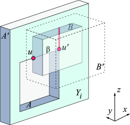
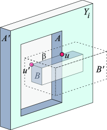
(a)	(b)

Figure 16: Case 4: $A$ is a dent behind $Y_{i}$, enclosed within protrusion $A^{\prime}$. $B$ is a dent in front of $Y_{i}$, enclosed within protrusion $B^{\prime}$.

Case 4. $A$ and $B$ are both dents: $A$ is a dent behind $Y_{i}$ enclosed within protrusion $A^{\prime}$, and $B$ is a dent in front of $Y_{i}$ enclosed within protrusion $B^{\prime}$ (see Fig. 16). The genus-zero assumption implies that $r(A)\cap r(B)$ is a polygonal region of positive area. Since $u\in r_{c}(A)\cap r_{c}(B)$, we have that $u\in r(A)\cap r(B)$. Let $\beta$ be the boundary segment of $r(A)\cap r(B)$ incident to $u$. We discuss two subcases:

1. $\beta\subset P^{-}$, meaning that $\beta\subset A$ (see Fig. 16a).

   An analysis similar to the one for the case illustrated in Fig. 15a (Case 3) shows that $A$ and $B$ are ray-connected, a contradiction.

2. $\beta\subset P^{+}$, meaning that $\beta\subset B$ (see Fig. 16b). We show that $A$ and $A^{\prime}$ are ray-connected, $B$ and $B^{\prime}$ are ray-connected, and $A^{\prime}$ and $B^{\prime}$ are ray-connected. This implies that $A$ and $B$ are ray-connected, a contradiction. First note that the ray-pair algorithm shoots a ray-pair $(r,r^{\prime})$ upward from a highest gridedge on $\beta$. An analysis similar to the one for the case illustrated in Fig. 13a (conceptually popping $B$ to become a protrusion) shows that $r$ and $r^{\prime}$ must hit $B$, thus ray-connecting $B$ and $B^{\prime}$. That $A$ and $A^{\prime}$ are ray-connected follows immediately from the fact that $r_{c}(A,A^{\prime})$ has a gridpoint higher than $u$, and similarly for $A^{\prime}$ and $B^{\prime}$.

Having exhausted all possible cases, the connectivity claim of the lemma is established. Because the proof for each of these cases goes through by considering either the first or second ray of a ray-pair, retaining either ray suffices to preserve connectivity. Thus the second claim of the lemma is established as well.

References

- [BDD+98] T. Biedl, E. Demaine, M. Demaine, A. Lubiw, J. O’Rourke, M. Overmars, S. Robbins, and S. Whitesides. Unfolding some classes of orthogonal polyhedra. In Proc. 10th Canad. Conf. Comput. Geom., pages 70–71, 1998.
- [DEE+03] E. D. Demaine, D. Eppstein, J. Erickson, G. W. Hart, and J. O’Rourke. Vertex-unfoldings of simplicial manifolds. In Andras Bezdek, editor, Discrete Geometry, pages 215–228. Marcel Dekker, 2003. Preliminary version appeared in 18th ACM Symposium on Computational Geometry, Barcelona, June 2002, pp. 237-243.
- [DFO06] M. Damian, R. Flatland, and J. O’Rourke. Grid vertex-unfolding orthogonal polyhedra. In Proc. 23rd Symp. on Theoretical Aspects of Comp. Sci., pages 264–276, February 2006. Lecture Notes in Comput. Sci., Vol. 3884, Springer.
- [DIL04] E. D. Demaine, J. Iacono, and S. Langerman. Grid vertex-unfolding of orthostacks. In Proc. Japan Conf. Discrete Comp. Geom., November 2004. To appear in LNCS, 2005.
- [DO05a] E. D. Demaine and J. O’Rourke. A survey of folding and unfolding in computational geometry. In J. E. Goodman, J. Pach, and E. Welzl, editors, Combinatorial and Computational Geometry, pages 167–211. Cambridge University Press, 2005.
- [DO05b] Erik D. Demaine and Joseph O’Rourke. Open problems from CCCG 2004. In Proc. 17th Canad. Conf. Comput. Geom., pages 303–306, 2005.
- [GBKK98] S. K. Gupta, D. A. Bourne, K. H. Kim, and S. S. Krishnan. Automated process planning for sheet metal bending operations. J. Manufacturing Systems, 17(5):338–360, 1998.
- [O’R00] Joseph O’Rourke. Folding and unfolding in computational geometry. In Discrete Comput. Geom., volume 1763 of Lecture Notes Comput. Sci., pages 258–266. Springer-Verlag, 2000. Papers from the Japan Conf. Discrete Comput. Geom., Tokyo, Dec. 1998.
- [PY92] M. S. Paterson and F. F. Yao. Optimal binary space partitions for orthogonal objects. J. Algorithms, 13:99–113, 1992.
- [SSW89] E. L. Schwartz, A. Shaw, and E. Wolfson. A numerical solution to the generalized map-maker’s problem: Flattening nonconvex poleyderal surfaces. IEEE Trans. Pattern Anal. Mach. Intell., 11(9):1005–1008, 1989.
- [THCM04] Marco Tarini, Kai Hormann, Paolo Cignoni, and Claudio Montani. Polycube-maps. ACM Trans. Graph., 23(3):853–860, 2004.
- [Wan97] C.-H. Wang. Manufacturability-driven decomposition of sheet metal products. PhD thesis, Carnegie Mellon University, The Robotics Institute, 1997.