Priority sampling estimating arbitrary subset sums

Abstract

Starting with a set of weighted items, we want to create a generic sample of a certain size that we can later use to estimate the total weight of arbitrary subsets. Applied to internet traffic analysis, the items could be records summarizing the flows of packets streaming by a router, with, say, a hundred records to be sampled each hour. A subset could be flow records of a worm attack whose signature is only determined after sampling has taken place. The samples taken in the past allow us to trace the history of the attack even though the worm was unknown at the time of sampling.

Estimation from the samples must be accurate even with heavy-tailed distributions where most of the weight is concentrated on a few heavy items. We want the sample to be weight sensitive, giving priority to heavy items. At the same time, we want sampling without replacement in order to avoid selecting heavy items multiple times. To fulfill these requirements we introduce priority sampling, which is the first weight sensitive sampling scheme without replacement that is suitable for estimating subset sums. Testing priority sampling on Internet traffic analysis, we found it to perform orders of magnitude better than previous schemes.

Priority sampling is simple to define and implement: we consider a steam of items $i=0,...,n-1$ with weights $w_{i}$. For each item $i$, we generate a random number $\alpha_{i}\in(0,1)$ and create a priority $q_{i}=w_{i}/\alpha_{i}$. The sample $S$ consists of the $k$ highest priority items. Let $\tau$ be the $(k+1)^{th}$ highest priority. Each sampled item $i$ in $S$ gets a weight estimate $\widehat{w}_{i}=\max\{w_{i},\tau\}$, while non-sampled items get weight estimate $\widehat{w}_{i}=0$.

Magically, it turns out that the weight estimates are unbiased, that is, $\textsf{E}[\widehat{w}_{i}]=w_{i}$, and by linearity of expectation, we get unbiased estimators over any subset sum simply by adding the sampled weight estimates from the subset. Also, we can estimate the variance of the estimates, and find, surprisingly, that the covariance between estimates $\widehat{w}_{i}$ and $\widehat{w}_{j}$ of different weights is zero.

Finally, we conjecture an extremely strong near-optimality; namely that for any weight sequence, there exists no specialized scheme for sampling $k$ items with unbiased weight estimators that gets smaller total variance than priority sampling with $k+1$ items. Very recently, Szegedy has settled this conjecture.

Key words

Subset sum estimation, weighted sampling, sampling without replacement.

1 Introduction

Starting with a set of weighted items, we want to create a generic sample of a certain size that we can later use to estimate the total weight of arbitrary subsets. Applied to internet traffic analysis, the items could be records summarizing the flows streaming by a router, with, say, a hundred records sampled each hour. A subset could be flow records of a worm attack whose signature is only determined after sampling has taken place. The samples taken in the past allow us to trace the history of the attack even though the worm was unknown at the time of sampling.

Estimation from the samples must be accurate even with heavy-tailed distributions where most of the weight is concentrated on a few heavy items. We want the sample to be weight sensitive, giving priority to heavy items. At the same time, we want sampling without replacement in order to avoid selecting heavy items multiple times. To fulfill these requirements we introduce priority sampling, which is the first weight sensitive sampling scheme without replacement that is suitable for estimating subset sums. Testing priority sampling on Internet traffic analysis, we found it to perform orders of magnitude better than previous schemes.

1.1 Priority Sampling

Priority sampling is a fundamental new technique to sample $k$ items from a stream of weighted items so as to later estimate arbitrary subset sums. The scheme is illustrated in Figure 1.

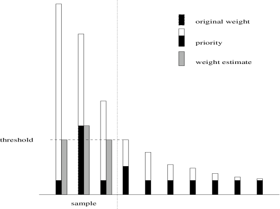
Figure 1: Priority sampling of size 3 from a set of 10 weighted items.

We consider a stream of items with positive weights $w_{0},...,w_{n-1}$. For each item $i=0,..,n-1$, we generate an independent uniformly random $\alpha_{i}\in(0,1)$, and a priority $q_{i}=w_{i}/\alpha_{i}$. Assuming that all priorities are distinct, the priority sample $S$ of size $k<n$ consists of the $k$ items of highest priority. An associated threshold $\tau$ is the $(k+1)^{\mathrm{th}}$ priority. Then $i\in S\iff q_{i}>\tau$. Each sampled item $i\in S$ gets a weight estimate $\widehat{w}_{i}=\max\{w_{i},\tau\}$. If $i\not\in S$, $\widehat{w}_{i}=0$. We will prove

$$\textsf{E}\left[{{\widehat{w}_{i}}}\right]=w_{i}$$ (1)

By linearity of expectation, if we want to estimate the total weight of an arbitrary subset $I\subseteq[n]=\{0,1,\ldots,n-1\}$, we just sum the corresponding weight estimates in the sample, that is,

$$\textsf{E}\left[{{\sum_{i\in S\cap I}\widehat{w}_{i}}}\right]=\sum_{i\in I}w_{i}$$ (2)

Ties between priorities happen with probability zero, and can be resolved arbitrarily. We resolve them in favor of earlier items. Thus we view priority $q_{i}$ as higher than $q_{j}$, denoted $q_{i}\succ q_{j}$, if either $q_{i}>q_{j}$ or $q_{i}=q_{j}$ and $i<j$. With any such resolution of ties, priority sampling works even if some weights are zero.

Note that in the case of unit weights, $\tau$ is just the $(k+1)^{\mathrm{th}}$ largest value $1/\alpha_{i}$, and then (2) simplifies to

$$\textsf{E}\left[{{k\tau}}\right]=n.$$ (3)

This unit case is a classic theorem in order statistics (see e.g., [2, 5]).

1.2 Selecting Subsets

We will now, with a few examples, illustrate how subsets could be selected. The basic point is that an item, besides the weight, has other associated information, and selection of an item may be based on all its associated information. To estimate the total weight of all selected items, we sum the weight estimates of all sampled items that would be selected. We note that the examples below could be based on any kind of sampling. What distinguishes priority sampling is the quality of the answers.

Internet traffic analysis

Our motivating application comes from Internet traffic analysis. Internet routers export information about transmissions of data passing through. These transmissions are called flows. A flow could be an ftp transfer of a file, an email, or some other collection of related data moving together. A flow record is exported with statistics such as summary information such as application type, source and destination IP addresses, and the number of packets and total bytes in the flow. We think of byte size as the weight.

We want to sample flow records in such a way that we can answer questions like how many bytes of traffic came from a given customer or how much traffic was generated by a certain application. Both of these questions ask what is the total weight of a certain selection of flows. If we knew in advance of measurement which selections were of interest, we could have a counter for each selection and increment these as flows passed by. The challenge here is that we must not be constrained to selections known in advance of the measurements. This would preclude exploratory studies, and would not allow a change in routine questions to be applied retroactively to the measurements.

A killer example where the selection is not known in advance was the tracing of the Internet Slammer worm [11]. It turned out to have a simple signature in the flow record; namely as being UDP traffic to port 1434 with a packet size of 404 bytes. Once this signature was identified, the historical development of the worm could be determined by selecting records of flows matching this signature from a data base of sampled flow records.

We note that data streaming algorithms have been developed that generalizes counters to provide answers to a range of selections such as, for example, range queries in a few dimensions [9]. However, each such method is still restricted to a limited type of selection to be decided in advance of the measurements.

External information in the selection

In our next example, suppose Wallmart saved samples of all their sales where each record contained information such as item, location, time, and price. Based on sampled records, they might want to ask questions like how many days of rain does it take before we get a boom in the sale of rain gear. Knowing this would allow them to tell how long the would need to order and disperse the gear if the weather report promissed a long period of rain. Now, the weather information was not part of the sales records, but if they had a data base with historical weather information, they could look up each sampled sales record with rain gear, and check how many days it had rained at that location before the sale.

The important lesson from this example is that selection can be based on external information not even imagined relevant at the time when measurements are made. Such scenarios preclude any kind of streaming algorithm based on selections of limitated complexity, and shows the inherent relevance of sampling preserving full records for the perpose of arbitrary selections.

1.3 Relation to classic sampling schemes

What distinguishes priority sampling is how well it does in the common case of a heavy tailed weight distribution [10]. The problem with uniform sampling is that it is likely to miss out on the small proportion of heavy items. An alternative is weighted sampling with replacement where each sample is chosen independently, each item being selected with probability proportional to its weight. The problem is that we are likely to get many duplicates of the heavy items, and hence provide less information on lighter items. A variant of weighted sampling with replacement for integer weights is to divide them into unit weights. This way we can get at most $w_{i}$ samples of units from item $i$. However, when weights are large compared with the number of samples, this is still very similar to the basic weighted sampling without replacement.

The above observations suggest that we need weight-sensitive sampling without replacement. For example, we can perform weighted sampling with replacement, but skip duplicates until we have the desired number of samples. The book [3] mentions 50 such schemes, but none of these provides estimates of sums. The basic problem is that the probability that a given item is included in the sample is a complicated function of all the involved weights.

Clearly priority sampling acts without replacement. To see that it is weight-sensitive, suppose we have an item $i$ which is $r=w_{j}/w_{i}\geq 1$ times smaller than an item $j$. Then the probability that $i$ gets higher priority than $j$ is $1/2r$. More precisely,

$$\Pr[q_{i}>q_{j}]=\Pr[w_{i}/\alpha_{i}>w_{j}/\alpha_{j}]=\Pr[\alpha_{i}<\alpha_{j}/r]=\int_{0}^{1}\alpha_{j}/r\;d\alpha_{j}=1/2r$$

Priority sampling is thus weight-sensitive without replacement, and, as stated in (2), it provides simple unbiased estimates of arbitrary sums. We will present tests of priority sampling on real Internet data, and see that estimating subset sums needs orders of magnitude fewer samples than uniform sampling and weighted sampling without replacement.

1.4 Outline of the Paper

The rest of the paper is organized as follows. In Section 2 we present the proof that priority sampling provides unbiased estimators as stated in (1). In addition we will show how we can estimate the variance of our subset sum estimates. This relies on the striking property of priority sampling that we establish, namely, that with more than one sample, the covariance between different weight estimates is zero. In Section 3 we compare our new priority sampling with threshold sampling from [7], a scheme which is very closely related but does not provide a specified number of samples. In Section 4, we present experiments with priority sampling on real data from the Internet, demonstrating orders of magnitude gain in accuracy in estimation weight sums, as compared with uniform sampling and weighted sampling without replacement. In Section 5, we analyze the performance of the different sampling schemes in some simple cases in order to gain further understanding of the experiments. In Section 6, we conjecture an extremely strong near-optimality; namely that for any weight sequence, there exists no specialized scheme for sampling $k$ items with unbiased weight estimators that gets smaller total variance than priority sampling with $k+1$ items. This conjecture was recently settled by Szegedy [12].q In Section 7, we show how we can maintain a priority sample of size $k$ for a stream of weighted items, spending only constant time on each item as it comes by. We finish with some concluding remarks in Section 8.

A preliminary version of parts of this work was published in a conference proceeding [6], including the basic announcement of the priority sampling scheme. Our original proof of (1) was based on the standard proofs for the known unit case [2, 5], but here we present a much simpler combinatorial proof and include an entirely new analysis of variance and covariance. The experiments reported here are all new, and so is most of the analysis of simple cases, as well as the conjecture concerning near-optimality.

2 Unbiased estimation with priority sampling

In this section, we will show that priority sampling yields unbiased estimates of subset sums as stated in (1). The proof is simpler and more combinatorial than the standard proofs for the known unit case [2, 5]. We will also show how to form unbiased estimators of secondary weights. Finally, we consider variance estimation. We show that there is no covariance between the weight estimates of different items, and that we can get unbiased estimates of the variance of any subset sum estimate.

Recall that we consider items with positive weights $w_{0},...,w_{n-1}$. For each item $i\in[n]$, we generate an independent uniformly distributed random number $\alpha_{i}\in(0,1)$, and a priority $q_{i}=w_{i}/\alpha_{i}$. Priority $q_{i}$ is higher than $q_{j}$, denoted $q_{i}\succ q_{j}$, if either $q_{i}>q_{j}$, or $q_{i}=q_{j}$ and $i<j$. A priority sample $S$ of size $k$ consists of the $k$ items of highest priority. The threshold $\tau$ is the $(k+1)^{\mathrm{st}}$ highest priority. Then $i\in S\iff q_{i}\succ\tau$. Each $i\in S$ gets a weight estimate $\widehat{w}_{i}=\max\{w_{i},\tau\}$. Also, for $i\not\in S$, we define $\widehat{w}_{i}=0$. Now (1) states that $\textsf{E}[\widehat{w}_{i}]=w_{i}$.

We will prove that (1) holds for an item $i$ no matter which values the other $\alpha_{j},\ j\neq i$ take. Fixing these values, we fix all the other priorities $q_{j},\ j\neq i$. Let $\tau^{\prime}$ be the $k^{\mathrm{th}}$ highest of these other priorities. We can now view $\tau^{\prime}$ as a fixed number. More formally, our analysis is conditioned on the event $A(\tau^{\prime})$ of $\tau^{\prime}$ being the $k^{\mathrm{th}}$ highest among the priorities $q_{j},\ j\neq i$, and we will prove

$$\textsf{E}[\widehat{w}_{i}|A(\tau^{\prime})]=w_{i}.$$ (4)

Proving (4) for any value of $\tau^{\prime}$ implies (1). The essential observation is as follows.

Lemma 1

Conditioned on $A(\tau^{\prime})$, item $i$ is picked with probability $\min\{1,w_{i}/\tau^{\prime}\}$, and if picked, $\tau=\tau^{\prime}$.

Proof

We pick $\alpha_{i}\in(0,1)$ uniformly at random, thus fixing $q_{i}=w_{i}/\alpha_{i}$. If $q_{i}\prec\tau^{\prime}$, there are at least $k$ priorities higher than $q_{i}$, so $i\not\in S$. Conversely, if $q_{i}\succ\tau^{\prime}$, then $\tau^{\prime}$ becomes the $(k+1)$th priority among all priorities, so $\tau^{\prime}=\tau$, and then $i\in S$. Finally,

$$\Pr\!\left[{{i\in S|A(\tau^{\prime})}}\right]=\Pr\!\left[{{q_{i}\succ\tau^{\prime}}}\right]=\Pr\!\left[{{\alpha_{i}<w_{i}/\tau^{\prime}}}\right]=\min\{1,w_{i}/\tau^{\prime}\}$$

 
From Lemma 1, we get

$$\textsf{E}[\widehat{w}_{i}|A(\tau^{\prime})] = \Pr\!\left[{{i\in S|A(\tau^{\prime})}}\right]\times\textsf{E}\left[{{\widehat{w}_{i}|i\in S\wedge A(\tau^{\prime})}}\right]$$

$$= \min\{1,w_{i}/\tau^{\prime}\}\times\max\{w_{i},\tau^{\prime}\}$$

$$= w_{i}$$

The last equality follows by observing that both the $\min$ and the $\max$ take their first, respectively their second value, depending on whether or not $w_{i}\geq\tau^{\prime}$. This completes the proof of (4), hence of (1)

2.1 Zero weight items and sampling it all

We note here that priority sampling, as defined above, works even in the presence of zero weights. First we note that $w_{i}=0\iff q_{i}=w_{i}/\alpha_{i}=0$ while $w_{i}>0\iff q_{i}=w_{i}/\alpha_{i}>w_{i}>0$. It follows that zero weight items can only be sampled if all positive weight items have been sampled. Moreover, if we do sample a zero weight item $i$, we have $\tau\prec q_{i}=w_{i}=0$, so $\tau=0$, and then $\widehat{w}_{j}=w_{j}$ for all items $j$. Having noted that zero weight items do not cause problems, we will mostly ignore them.

Above we have assumed $k<n$, but we note a natural view of a priority sample of everything, that is, with $k=n$. We define an $(n+1)^{th}$ priority $\tau=q_{n}=0$, as if we had an extra zero weight $w_{n}=0$. Then $q_{i}\succ\tau=q_{n}$ for all $i\in[n]$, so all items get sampled. Moreover $\widehat{w}_{i}=\max\{w_{i},\tau\}=w_{i}$, so the weight estimate is equal to the original weight.

2.2 Secondary variables

Suppose that each item $i$ has a secondary variable $x_{i}$. We can then use (1) to give unbiased estimators of corresponding secondary subset sums. More precisely, we set $\widehat{x}_{i}=\widehat{w}_{i}x_{i}/w_{i}$. That is $\widehat{x}_{i}=\max\{w_{i},\tau\}x_{i}/w_{i}=\max\{1,\tau/w_{i}\}x_{i}$ if $i$ is sampled; $0$ otherwise. Then (1) implies $\textsf{E}[\widehat{x}_{i}]=x_{i}$.

An application could be to deal with negative and positive weights $x_{i}$. We could define the priority weights as their absolute values, that is, $w_{i}=|x_{i}|$, and use these non-negative weights in the priority sample.

Another application could be if we had several different variables for each item. Instead of making an independent priority sample for each variable, we could construct a compromise weight. For example, for each item, the weight could be a weighted sum of all the associated variables.

2.3 Variance estimation for a single item

We now provide a simple variance estimator

$$\widehat{v}_{i}=\left\{\begin{array}[]{ll}w_{i}\tau\max\{0,\tau-w_{i}\}&\mbox{if }i\in S\\ 0&\mbox{if }i\not\in S\end{array}\right.\textnormal{,}$$

and show that it is unbiased, that is,

$$\textsf{E}\left[{{\widehat{v}_{i}}}\right]=\mathop{\sf Var}[\widehat{w}_{i}].$$ (5)

As in the proof of (1), we define $A(\tau^{\prime})$ to be the event that $\tau^{\prime}$ is the $k^{\mathrm{th}}$ highest among the priorities $q_{j},\ j\neq i$. We will prove

$$\textsf{E}\left[{{\widehat{v}_{i}|A(\tau^{\prime})}}\right]=\textsf{E}[\widehat{w}_{i}^{2}|A(\tau^{\prime})]-w_{i}^{2}.$$ (6)

From Lemma 1, we get

$$\textsf{E}[\widehat{v}_{i}|A(\tau^{\prime})] = \Pr\!\left[{{i\in S|A(\tau^{\prime})}}\right]\times\textsf{E}\left[{{\widehat{v}_{i}|i\in S\wedge A(\tau^{\prime})}}\right]$$

$$= \min\{1,w_{i}/\tau^{\prime}\}\times\tau^{\prime}\max\{0,\tau^{\prime}-w_{i}\}$$

$$= \max\{0,w_{i}\tau^{\prime}-w_{i}^{2}\}.$$

On the other hand,

$$\textsf{E}[\widehat{w}_{i}^{2}|A(\tau^{\prime})] = \Pr\!\left[{{i\in S|A(\tau^{\prime})}}\right]\times\textsf{E}\left[{{\widehat{w}_{i}^{2}|i\in S\wedge A(\tau^{\prime})}}\right]$$

$$= \min\{1,w_{i}/\tau^{\prime}\}\times\max\{w_{i},\tau^{\prime}\}^{2}$$

$$= \max\{w_{i}^{2},w_{i}\tau^{\prime}\}.$$

This establishes (6) and hence (5).

2.4 Covariance

Assuming that we sample more than one item, we will show that the covariance between our weight estimates is zero , that is, for $k>1$ and $i\neq j$,

$$\textsf{E}\left[{{\widehat{w}_{i}\widehat{w}_{j}}}\right]=w_{i}w_{j}$$ (7)

If $k=1$, we have $\textsf{E}\left[{{\widehat{w}_{i}\widehat{w}_{j}}}\right]=0$ since we cannot sample both $i$ and $j$.

Note that (7) is somewhat counter-intuitive in that if we sample $i$ then this reduces the probability that we also sample $j$. However, the assumption that $i$ is sampled affects the threshold $\tau$ and thereby the weight estimate $\widehat{w}_{j}$ and somehow, the different effects cancel out.

We will prove (7) via the following common generalization of (7) and (1) holding for any $I\subset[n],\ |I|\leq k$:

$$\textsf{E}\left[{{\prod_{i\in I}\widehat{w}_{i}}}\right]=\prod_{i\in I}w_{i}$$ (8)

If $|I|>k$, we have $\textsf{E}\left[{{\prod_{i\in I}\widehat{w}_{i}}}\right]=0$ since at most $k$ items are sampled with $\widehat{w}_{i}>0$.

The proof of (8) generalizes that of (1). Inductively on the size of $I$, we will prove that (8) holds no matter what values all the other $\alpha_{j}$, $j\not\in I$ take. The equality is trivially true in the base case where $I=\emptyset$ and the products equals one.

Thus, for all $j\not\in I$, fix all $\alpha_{j}\in(0,1)$ and priorities $q_{j}=w_{j}/\alpha_{j}$. Fix $\tau^{\prime\prime}$ to be the $(k-|I|+1)^{\mathrm{th}}$ highest of these priorities $q_{j}\ j\not\in I$. This priority exists because $k\leq|I|<n$. Next for $i\in I$, we pick $\alpha_{i}\in(0,1)$ and set $q_{i}=w_{i}/\alpha_{i}$. We can now have at most $(k-|I|)+|I|$ priorities below $\tau^{\prime\prime}$, so $\tau^{\prime\prime}$ is at least as big as our new threshold $\tau$.

Consider the case that $I$ has a weight $w_{h}\geq\tau^{\prime\prime}$. Fix $\alpha_{h}\in(0,1)$ arbitrarily. Then $q_{h}>w_{j}\geq\tau^{\prime\prime}\geq\tau$, so item $h$ is sampled with $\widehat{w}_{h}=\max\{w_{h},\tau\}=w_{h}$. Hence $\textsf{E}\left[{{\prod_{i\in I}\widehat{w}_{i}}}\right]=w_{h}\textsf{E}\left[{{\prod_{i\in I\setminus\{m\}}\widehat{w}_{i}}}\right]$. We have now fixed all $\alpha_{j}$, $j\not\in I\setminus\{m\}$, and by induction, $\textsf{E}\left[{{\prod_{i\in I\setminus\{m\}}\widehat{w}_{i}}}\right]=\prod_{i\in I\setminus\{m\}}w_{i}$. This completes the proof of (8) in the case that $w_{h}\geq\tau^{\prime\prime}$.

Next consider the case that all weights from $I$ are smaller than $\tau^{\prime\prime}$. Let $q_{\ell}$ be the lowest priority from $I$. If $q_{\ell}\prec\tau^{\prime\prime}$, then there are at least $(k-|I|+1)+|I\setminus\{\ell\}|=k$ priorities higher than $q_{\ell}$, so $q_{\ell}\not\in S$, and $\widehat{w}_{\ell}=0=\prod_{i\in I}\widehat{w}_{i}$. Thus, if $q_{\ell}\prec\tau^{\prime\prime}$, there is no contribution to $\textsf{E}\left[{{\prod_{i\in I}\widehat{w}_{i}}}\right]$.

Conversely, if $q_{\ell}\prec\tau^{\prime\prime}$, then all priorities from $I$ are bigger than $\tau^{\prime\prime}$. In this case there are exactly $(k-|I|)+|I|=k$ priorities higher than $\tau^{\prime\prime}$, so $\tau^{\prime\prime}$ becomes our threshold $\tau$. Then each $i\in S$ are sampled. Since $w_{i}\leq\tau^{\prime\prime}=\tau$, we get $\widehat{w}_{i}=\max\{w_{i},\tau\}=\tau$. Hence $\prod_{i\in I}\widehat{w}_{i}={\tau^{\prime\prime}}^{|}I|$. Since no weights in $I$ is higher than $\tau^{\prime\prime}$, the probability that all their priorities are bigger is $\prod_{i\in I}(w_{i}/\tau^{\prime\prime})$. Thus, the contribution to $\textsf{E}\left[{{\prod_{i\in I}\widehat{w}_{i}}}\right]$ is ${\tau^{\prime\prime}}^{|}I|\prod_{i\in I}(w_{i}/\tau^{\prime\prime})=\prod_{i\in I}w_{i}$. This completes the proof of (8) in the remaining case where $w_{h}<\tau^{\prime\prime}$.

2.5 Variance estimation over any subset

We can now use our variance estimator from Section 2.3 to estimate the variance over any subset. By (7) and (5) we get an unbiased estimator of the variance of any subset sum estimate simply by summing the variance estimators from the subset, that is, if $k>1$ for any subset $I\subseteq[n]$,

$$\mathop{\sf Var}[\sum_{i\in S\cap I}\widehat{w}_{i}]=\textsf{E}\left[{{\sum_{i\in S\cap I}\widehat{v}_{i}}}\right]$$ (9)

In fact, (9) also holds if $k=1$, but this is because $\mathop{\sf Var}[\sum_{i\in S\cap I}\widehat{w}_{i}]=\infty$ for any non-empty subset $I$. We shall return to this point later in Section 5.1.

3 Comparison with a fixed threshold scheme

It is instructive to compare our priority sampling scheme with threshold sampling from [7]. In that approach each item is sampled independently, so we do not control the exact number of samples. Before sampling, a fixed threshold $\tau^{THR}$ is chosen. An item $i$ is sampled if $w_{i}\geq\tau^{THR}$, or with probability $w_{i}/\tau^{THR}$ if $w_{i}\leq\tau^{THR}$. We denote the set of selected items by $S^{THR}$.

To see the relation to priority sampling, note that threshold sampling can be expressed in a manner similar to priority sampling as follows: generate a random number $\alpha_{i}\in(0,1]$ and sample item $i$ if $q_{i}=w_{i}/\alpha_{i}>\tau^{THR}$. As in our new scheme, the sampled items get weight estimate $\widehat{w}_{i}^{THR}=\max\{w_{i},\tau^{THR}\}$ whereas $\widehat{w}_{i}^{THR}=0$ if $i\not\in S^{THR}$. Thus the only difference between priority sampling and the threshold sampling from [7] is in the choice of the threshold. In threshold sampling, the threshold is fixed independent of the random choices. Thus the threshold determines only the expected number of independent samples, not the actual random number of samples. By contrast, in priority sampling, the threshold is picked depending on the random choices so as to get a fixed number of dependent samples. We note that it is far from obvious that such a threshold could be chosen without violating the unbiasedness of estimation.

3.1 Optimality of the fixed threshold scheme

In [7], the fixed threshold approach to independent sampling is proved to give an optimal trade-off between variance and sampling rate. More for an item $i$ with weight $w_{i}$, we have to decide on a sampling probability $p_{i}$. If $i$ is not picked, the weight estimate is zero, that is, $\widehat{w}_{i}(p_{i})=0$. To get an unbiased estimator, if item $i$ is picked, it should have weight estimate $\widehat{w}_{i}(p_{i})=w_{i}/p_{i}$. Then $\textsf{E}\left[{{\widehat{w}_{i}(p_{i})}}\right]=w_{i}$. Generally, we want to sample few items, yet keep the variance low. This motivates an objective of the form

$$\mbox{minimize }p_{i}+\beta\,\mathop{\sf Var}\left[{{\widehat{w}_{i}(p_{i})}}\right]$$

Here

$$\mathop{\sf Var}\left[{{\widehat{w}_{i}(p_{i})}}\right]=\textsf{E}\left[{{(\widehat{w}_{i}(p_{i}))^{2}}}\right]-w_{i}^{2}\mbox{ where }\textsf{E}\left[{{(\widehat{w}_{i}(p_{i}))^{2}}}\right]=p_{i}(w_{i}/p_{i})^{2}=w_{i}^{2}/p_{i}.$$

Thus we want to

$$\mbox{minimize }p_{i}+\beta\,w_{i}^{2}/p_{i}$$

For $p_{i}\in[0,1]$, the solution is to set $p_{i}=\min\{1,\sqrt{\beta}w_{i}\}$. With $\sqrt{\beta}=1/\tau^{THR}$ this is equivalent to the fixed threshold scheme. That is, for any choice of $\tau^{THR}$, the fixed threshold scheme picks the $p_{i}=\max\{1,w_{i}/\tau^{THR}\}$ so as to

$$\mbox{minimize }p_{i}+(1/\tau^{THR})^{2}\mathop{\sf Var}\left[{{\widehat{w}_{i}(p_{i})}}\right].$$ (10)

Summing over the whole stream of items, we

$$\mbox{minimize }\sum_{i\in[n]}\left(p_{i}+(1/\tau^{THR})^{2}\mathop{\sf Var}\left[{{\widehat{w}_{i}(p_{i})}}\right]\right)=\sum_{i\in[n]}p_{i}+1/(\tau^{THR})^{2}\mathop{\sf Var}\left[{{\sum_{i\in[n]}\widehat{w}_{i}(p_{i})}}\right]$$ (11)

We now constrain ourselves to getting an expected number $k$ of samples. To minimize the total variance, we just have to identify $\tau^{THR}$ such that

$$\sum_{i\in[n]}{p_{i}}=\sum_{i\in[n]}\min\{1,w_{i}/\tau^{THR}\}=k$$

With this value of $\tau^{THR}$, the fixed threshold scheme from [7] minimizes the total variance subject to unbiased estimation and an expected number $k$ of samples. Any other assignments of individual sampling probabilities $p_{i}$ will do worse. The quality of our new scheme is largely inherited from this fixed threshold scheme, but we have some extra variability due to the variability of the threshold.

4 Experiments

We tested priority sampling on 10 minutes of flows from an Internet gateway router. For increasing sample sizes, we wanted to check our ability to estimate subset sums where each subset was defined by flows originated by certain applications such as FTP and web traffic. This illustrates how priority sampling can be used today in a backbone network. The basic flow statistics for the different applications is presented in Table 1.

application	bytes	% of traffic	# flows	% flows	max flow size	average	min
all	4265677642	100.00	85680	100.00	3372865057	49786	28
ftp	3394832734	79.58	727	0.84	3372865057	4669646	40
web	80120429	1.87	7787	9.08	3139196	10289	40
dns	4083277	0.09	40767	47.58	621812	100	40

Table 1: Statistics on ten minutes of flows from an Internet gateway router showing traffic from some different applications. Note that nearly half the flows belong to applications not mentioned.

We compared the following sampling schemes:

PRI

our new priority sampling.

U$-$R

uniform sampling without replacement.

W$+$R

weighted sampling with replacement.

THR

the fixed threshold sampling from [7] as described in Section 3.

For weighted sampling with replacement, we note that there are two alternative ways of deriving weight estimates. More precisely, we have a list $S^{W+R}$ of $k$ samples. Each sample $S^{W+R}[j]$ is independent and equals item $i$ with probability $w_{i}/W$ where $W$ is the total weight. The simplest unbiased estimator of $w_{i}$ counts duplicates, estimating $w_{i}$ as $|\{j|S^{W+R}[j]\}|W/k$. However, we get a smaller variance if we just consider whether item $i$ is present in $S^{W+R}$. The probability of this event is

$$p_{i}^{W+R}=1-(1-w_{i}/W)^{k},$$

and then we get the unbiased weight estimator:

$$\widehat{w}_{i}^{W+R}=\left\{\begin{array}[]{ll}w_{i}/p_{i}^{W+R}&\mbox{if }i\in S^{W+R}\\ 0&\mbox{otherwise}\end{array}\right.$$

We now describe the setup of the experiments; the interpretation of the results follows in the next sections. In Figure 2 we compare the estimation accuracy of the different sampling schemes on the data summarized in Table 1. For each sampling scheme, we progressively increased the size of sample by selecting more items from the data, estimating total weight in each application subset of the total flows for each sample size.

In Figure 3, the same samples are used to estimate an $8\times 8=64$ entry traffic matrix. Each matrix element corresponds to the traffic between an input and output interface on a router. We estimate the total bytes for each matrix element. Our accuracy measure is average over all elements of the relative estimation error.

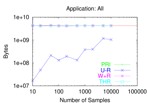
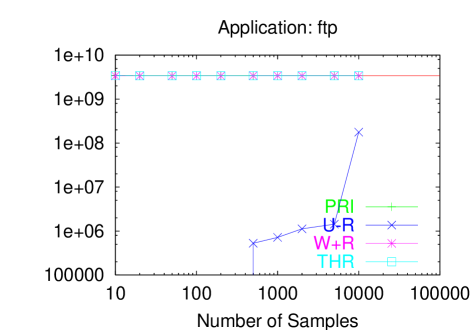
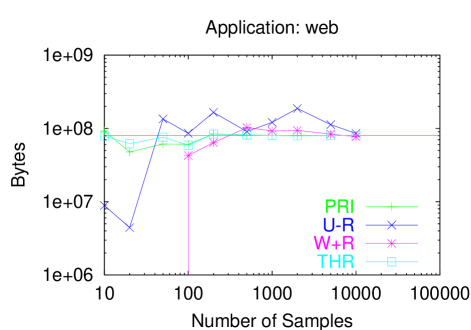
Figure 2: Estimating traffic from different applications with different sampling strategies. The red line shows the true traffic from each application.

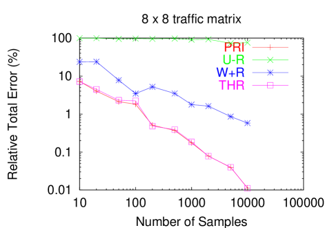
Figure 3: Estimating a traffic matrix with different sampling strategies. We divide the total error over all entries with the total traffic.

For priority sampling (PRI), uniform sampling without replacement (U$-$R), and weighted sampling with replacement (W$+$R), the number $k$ of samples is exact.

In threshold sampling (THR), the threshold determines only the expected number of samples. For each item $i$, we used the same priority $q_{i}=w_{i}/\alpha_{i}$ for priority sampling and threshold sampling. In priority sampling, we picked exactly $k$ samples using the $(k+1)^{th}$ priority $\tau$ as a threshold. In threshold sampling, we computed the threshold $\tau^{THR}$ giving an expected number $k$ of samples. Thus, for a given $k$, the only difference is in the choice of threshold.

Finally, Figure 4 tells the number of distinct samples as a percentage of the target. For priority sampling (PRI) and uniform sampling (U$-$R) we have no replacement, so we get exactly $k$ distinct samples, that is, 100%. With weighted sampling with replacements (W$+$R) the duplicates mean that we get less distinct samples. Finally, with threshold sampling (THR), all samples are distinct, but we only have an expected number $k$ of samples, hence the deviation from the target $k$.

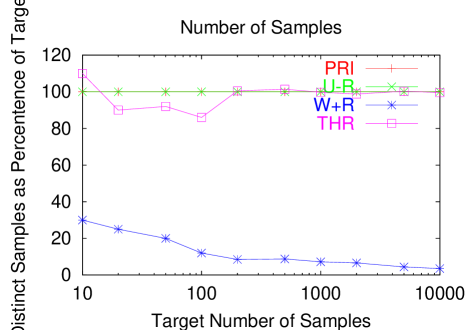
Figure 4: Number of distinct samples as percentage of target $k$.

4.1 Discussion

The quality of a sampling scheme is the number of samples it takes before the estimates converges towards the true value.

4.1.1 Sampling exactly $k$ samples

First we compare our priority sampling (PRI) scheme with the other schemes providing an exact number $k$ of samples, that is, with uniform sampling without replacement (U$-$R) and weighted sampling without replacement (W$+$R). In Figure 2 and  3, we see that priority sampling provides very substantial gains in accuracy over the other schemes.

When comparing the curves, there are two points to consider. One is how many samples it takes before we get one from a given application. This is the point at which we get our first non-zero estimates. Second we consider how quickly we converge after this point.

Number of samples needed to hit an application

With uniform sampling, the number of samples expected before we get one from a given application is roughly the total number of flows divided by the number of application flows. In that regard, ftp traffic is clearly the worst.

With weighted sampling without replacement, the expected number is roughly the total traffic divided by the application traffic. The worst application here is dns traffic which was the best application for uniform sampling.

Priority sampling is like weighted sampling without replacement but it avoids making duplicates of dominant items. If the dominant items are outside the application, we waste at most one sample on each. The impact is clear for dns traffic where we get the first sample about 30 times earlier with priority sampling than we did with weighted sampling without replacement. A more direct illustration of the problem is found in Figure 4 where we see how the fraction of distinct samples drops in weighted sampling without replacement.

Convergence after first hitting an application

After we have started getting samples from an application, uniform sampling may still have problems with convergence. This typically occurs if the weight distribution within the application is heavy-tailed. Once again, ftp traffic is the worst application, this time because it has a dominant flow with more than 99% of its traffic. Until this flow is sampled, we expect to underestimate. If it is sampled early, we will hugely overestimate, although this is unlikely. The typical heavy-tail behavior is that the estimate grows as we catch up with more and more dominant items. We see this phenomena both for ftp traffic and for all traffic combined.

With weighted sampling without replacement and with priority sampling, we get quicker convergence as soon as we start having samples from an application. Neither scheme has any problems with skewed weight distributions within the applications. For example, we see that weighted sampling without replacement starts slower than uniform on web traffic, yet it ends up converging faster. Similarly, priority sampling starts slower than uniform on dns traffic, yet it converging faster.

The traffic matrix

Figure 3 shows the average relative error over $8\times 8=64$ entries. We note first the poor performance of uniform sampling. In fact, it is only luck that the error with uniform is remains below 100%. This is because we miss the dominant items and get under-estimates that can never be by more than 100%. We could instead have gotten a dominant item early, leading to a huge over-estimate by far more than 100%.

Comparing priority sampling with weighted sampling without replacement the faster convergence of priority sampling is very clear. For example, priority sampling gets down around a 1% error with about 150 samples whereas weighted sampling with replacement needs about 3000 samples, and the weighted sampling falls further behind with smaller errors because it gets more and more duplicates.

4.2 Priority sampling versus threshold sampling

A reason to believe that priority sampling works very well for a fixed number of samples is its similarity with threshold sampling which for an expected number of independent samples minimized the total variance. In Figure 2 and 3 we see that indeed priority sampling (PRI) and threshold sampling (THR) are very close; neither having a systematic advantage. Hence, in our experiment, we see now loss in quality going from an expected number of samples (THR) to an exact number of samples (PRI). The variation in the actual number of samples with THR shown in Figure 4.

As we shall see below, there are certain boundary phenomena that makes priority sampling perform significantly worse than threshold sampling.

5 Analytic comparison of variance in some simple cases

In this section, we will compare the different sampling schemes on some simple cases where we can analyze the variance, so as to gain some intuition for what is going on.

Generalizing notation from Section 3, if $w$ is a weight and $p\in[0,1]$ a sampling probability, we let $\widehat{w}(p)$ denote the random variable that is $w/p$ with probability $p$; $0$ otherwise. Then

$$\textsf{E}\left[{{\widehat{w}(p)}}\right] = w$$

$$\textsf{E}\left[{{(\widehat{w}(p))^{2}}}\right] = p(w/p)^{2}=w^{2}/p$$

$$\mathop{\sf Var}\left[{{\widehat{w}(p)}}\right] = w^{2}/p-w^{2}=w^{2}\frac{1-p}{p}$$

It is also convenient to define the function

$$v(w,\tau)=w\max\{0,\tau-w\}$$

Then, with fixed threshold $\tau^{THR}$, the variance for item $i$ is

$$\mathop{\sf Var}[\widehat{w}_{i}^{THR}] = \mathop{\sf Var}\left[{{\widehat{w}_{i}(\max\{1,w_{i}/\tau^{THR}\})}}\right]$$

$$= w_{i}^{2}(1/\max\{1,w_{i}/\tau^{THR}\}-1)$$

$$= w_{i}\max\{0,\tau-w_{i})$$

$$= v(w_{i},\tau^{THR})$$

With our new priority sampling, the threshold changes, and the variance of item $i$ is

$$\mathop{\sf Var}\left[{{\widehat{w}_{i}}}\right]=\int_{\tau^{\prime}=0}^{\infty}f(\tau^{\prime})v(w_{i},\tau^{\prime})\,d\tau^{\prime}$$ (12)

where $f(\tau^{\prime})$ is the probability density function for $\tau^{\prime}$ to be the $k^{th}$ threshold amongst the items $j\neq i$. With $\tau^{\prime}$ thus defined, by Lemma 1, item $i$ is picked if $q_{i}=w_{i}/\alpha_{i}>\tau^{\prime}$ with $\widehat{w}_{i}=\tau^{\prime}$; $0$ otherwise. This imitates the fixed threshold scheme with $\tau^{\prime}=\tau^{THR}$. Thus (12) follows from the previous calculation with a fixed threshold.

Sometimes it is easier with a more direct calculation. Summing over all $j\neq i$, we integrate over choices of $\alpha_{j}$, multiply with the probability that $q_{j}=w_{j}/\alpha_{j}$ is the $k$th highest priority from $[n]\setminus\{i\}$, and multiply with the variance $v(w_{i},q_{j})$. That is,

$$\mathop{\sf Var}\left[{{\widehat{w}_{i}}}\right]=\sum_{j\in[n]\setminus\{i\}}\int_{0}^{1}\Pr\!\left[{{|\{h\in[n]\setminus\{i,j\}|q_{h}\succ q_{j}\}|=k-1}}\right]v(w_{i},q_{j})\;d\alpha_{j}$$ (13)

5.1 Infinite variance with single priority sample

We will show that if we only make a single priority sample with $k=1$, then the variance of any weight estimate is infinite. The proof is based on (13). We assume $i=0$. For a lower-bound, in the sum, we only need to consider one other item $j=1$. Also, when integrating over $\alpha_{1}$, we only consider very small values of $\alpha_{1}$. More precisely, define $\varepsilon=w_{1}/(2W)$ where $W$ is the sum of all weights. If $\alpha_{1}<\varepsilon$, we have $q_{1}=w_{1}/\alpha_{1}>2W$, and then

$$\Pr\!\left[{{|\{h\in[n]\setminus\{i,j\}|q_{h}\succ q_{j}\}|=k-1}}\right] = \Pr\!\left[{{|\{h\in\{2,...,n-1\}|q_{h}\succ q_{1}\}|=0}}\right]$$

$$> 1-\sum_{h\in\{2,...,n-1\}}\Pr\!\left[{{q_{h}>2W}}\right]$$

$$= 1-\sum_{h\in\{2,...,n-1\}}(w_{h}/2W)$$

$$> 1/2$$

Moreover

$$v(w_{i},q_{j})=v(w_{0},q_{1})=w_{0}\max\{0,w_{1}/\alpha_{1}-w_{0}\}>w_{1}/(2\alpha_{1})$$

Thus, by (13), we have

$$\mathop{\sf Var}\left[{{\widehat{w}_{0}}}\right]>\int_{0}^{\varepsilon}1/2\cdot w_{1}/(2\alpha_{1})\;d\alpha_{1}=\infty$$

We note that none of the other sampling schemes considered can get infinite variance.

Next, we argue that the variance is bounded if we make at least two priority samples. Again, we focus on the variance for item $i=0$. Also, it suffices to show that the integral in (13) is finite for each value of $j$, that is, we want to show that

$$V_{i,j}=\int_{0}^{1}\Pr\!\left[{{|\{h\in[n]\setminus\{i,j\}|q_{h}\succ q_{j}\}|=k-1}}\right]v(w_{i},q_{j})\;d\alpha_{j}$$

is bounded. Now, for $k\geq 2$,

$$\Pr\!\left[{{|\{h\in[n]\setminus\{i,j\}|q_{h}\succ q_{j}\}|=k-1}}\right] \leq \Pr\!\left[{{|\{h\in[n]\setminus\{i,j\}|q_{h}\succ q_{j}\}|\geq 1}}\right]$$

$$\leq \sum_{h\in[n]\setminus\{i,j\}}\Pr\!\left[{{q_{h}\succ q_{j}}}\right]$$

$$\leq \sum_{h\in[n]\setminus\{i,j\}}\Pr\!\left[{{w_{h}/\alpha_{h}>w_{j}/\alpha_{j}}}\right]$$

$$= \sum_{h\in[n]\setminus\{i,j\}}\min\{1,w_{h}\alpha_{j}/w_{j}\}$$

$$\leq \sum_{h\in[n]\setminus\{i,j\}}(w_{h}\alpha_{j}/w_{j})$$

$$< W\alpha_{j}/w_{j}$$

Moreover,

$$v(w_{i},q_{j})=w_{i}\max\{0,w_{j}/\alpha_{j}-w_{i}\}\leq w_{i}w_{j}/\alpha_{j}\textnormal{,}$$

so we get that

$$V_{i,j}<\int_{0}^{1}W\alpha_{j}/w_{j}\cdot w_{i}w_{j}/\alpha_{j}\,d\alpha_{j}=\int_{0}^{1}Ww_{i}\;d\alpha_{j}=Ww_{i}.$$

Hence

$$\mathop{\sf Var}\left[{{\widehat{w}_{i}}}\right]=\sum_{j\in[n]\setminus\{i\}}V_{i,j}<n\,Ww_{i},$$

so indeed the variance is bounded. Since the covariance is zero, it also follows that estimates of weights of subsets are bounded. Thus we have proved

Proposition 2

If we make a single priority sample, then all weight estimates have infinite variance. With more than one priority samples, all weight estimates are finite.

By contrast, with all the other sampling schemes, the variance estimates are finite as soon as we make at least one sample.

5.2 Unit weights

We will now study identical unit weights, focusing on the first item $i=0$. We will compute the exact variance for each of the sampling schemes considered.

Uniform sampling without replacement

For uniform sampling without replacement, item $0$ is picked with probability $p_{0}^{U-R}=k/n$, hence with

$$\mathop{\sf Var}\left[{{{\widehat{w}_{0}^{U-R}}}}\right]=\frac{1-p_{0}^{U-R}}{p_{0}^{U-R}}=\frac{n-k}{k}$$

Weighted sampling without replacement

For weighted sampling with replacement, item $0$ is picked with probability $p_{0}^{W+R}=1-(1-1/n)^{k}$, hence with

$$\mathop{\sf Var}\left[{{{\widehat{w}_{0}^{W+R}}}}\right]=\frac{1-p_{0}^{W+R}}{p_{0}^{W+R}}=\frac{(1-1/n)^{k}}{1-(1-1/n)^{k}}$$

For $k\ll n$, the variance approaches $\frac{n-k}{k}$ from above. However, for $k=n$, the variance approaches $1/(e(1-e^{-1})=0.58..$.

Fixed threshold

In the fixed threshold scheme from [7], we set $\tau^{THR}=n/k$. Then

$$\mathop{\sf Var}\left[{{\widehat{w}_{0}^{THR}}}\right]=v_{0}(\tau^{THR})=w_{1}\max\{0,\tau^{THR}-w_{i}\}=\frac{n-k}{k}$$ (14)

Priority sampling

For priority sampling, we will evaluate (13) exactly. We use that

$$\Pr\!\left[{{q_{h}\succ q_{1}}}\right]=\Pr\!\left[{{\alpha_{h}<\alpha_{1}}}\right]=\alpha_{1}$$

and

$$v_{0}(q_{1})=w_{0}\max\{0,q_{1}-w_{0}\}=(1/\alpha_{1}-1)$$

so

$$\mathop{\sf Var}\left[{{\widehat{w}_{0}}}\right] = \sum_{j=1}^{n-1}\int_{0}^{1}\Pr\!\left[{{|\{h\in\{2,...,n-1\}|q_{h}\succ q_{1}\}|=k-1}}\right]v_{0}(q_{1})\;d\alpha_{1}$$

$$= (n-1)\int_{\alpha_{1}=0}^{1}\Pr\!\left[{{B(n-1,\alpha)=k-1}}\right](1/\alpha_{1}-1)\;d\alpha_{1}$$

$$= (n-1)\int_{\alpha_{1}=0}^{1}{n-1\choose k-1}\alpha_{1}^{k-2}(1-\alpha_{1})^{n-k+1}\;d\alpha_{1}$$

$$= \frac{n-k}{k-1}$$

Discussion

For unit weights, uniform sampling without replacement and threshold sampling gets the sample variance on single item weight estimates; namely $\frac{n-k}{k}$. When $k$ is not too small, priority sampling gets nearly the same variance; namely $\frac{n-k}{k-1}$. Weighted sampling with replacement starts doing well, but gets worse and worse as $k$ grows. In particular, for any $k\geq n$, it has positive variance while all the other schemes have zero variance since they have no replacement.

5.3 Large and small weights

In this section we illustrate what happens when different weights are involved. We consider the case where we have $\ell$ large weights of weight $N$ and $n$ unit weights. The large weights are first, that is, $w_{0}=\cdots=w_{\ell-1}=N$ while $w_{\ell}=\cdots=w_{n+\ell-1}=1$. We let $W=\ell N+n$ denote the total weight. We view $\ell$, $n$, and $N$ as unbounded. We assume $\ell\ll n\ll\sqrt{N}$ and that $k\ll n$. These assumptions will help simplifying the analysis. We will use $w_{0}$ as a representative for the large items and $w_{n}$ as a representative for the small items. The results variances from the different sampling schemes will be accumulated in Table 2.

Uniform sampling without replacement

For uniform sampling without replacement, the large item $0$ is picked with probability $p_{0}^{U-R}=k/(n+\ell)$, hence with

$$\mathop{\sf Var}\left[{{{\widehat{w}_{0}^{U-R}}}}\right]=N^{2}\frac{1-p_{0}^{U-R}}{p_{0}^{U-R}}=N^{2}\frac{n+\ell-k}{k}\approx N^{2}\frac{n}{k}.$$

For small item $n$, we have the same sampling probability, $p_{n}^{U-R}=k/(n+\ell)$, so we get

$$\mathop{\sf Var}\left[{{{\widehat{w}_{n}^{U-R}}}}\right]=\frac{1-p_{n}^{U-R}}{p_{n}^{U-R}}\approx\frac{n}{k}.$$

Weighted sampling with replacement

For weighted sampling with replacement, the large item $0$ is picked with probability $p_{0}^{W+R}=1-(1-N/W)^{k}\approx 1-e^{-k/\ell}$ hence with

$$\mathop{\sf Var}\left[{{\widehat{w}_{n}^{W+R}}}\right]=N^{2}\frac{1-p_{0}^{W+R}}{p_{0}^{W+R}}\approx N^{2}\frac{e^{-k/\ell}}{1-e^{-k/\ell}}=N^{2}/(e^{k/\ell}-1).$$

In particular, this is $\Theta(N^{2})$ for $k=\Theta(\ell)$. Yet it saves a factor $n$ over uniform sampling with replacement in the case of large weights.

For weighted sampling with replacement, the small item $i=n$ is picked with probability $p_{n}^{W+R}=1-(1-1/W)^{k}\approx k/W\approx k/(\ell N)\ll 1$, hence with

$$\mathop{\sf Var}\left[{{\widehat{w}_{n}^{W+R}}}\right]=\frac{1-p_{n}^{W+R}}{p_{n}^{W+R}}\approx\ell N/k$$

Fixed threshold

For the fixed threshold scheme, if $k\leq\ell$, we set $\tau^{THR}=W/k>N$. Then for heavy item $0$,

$$\mathop{\sf Var}\left[{{\widehat{w}_{0}^{THR}}}\right]=v(w_{0},\tau^{THR})=N(W/k-N)\approx N^{2}\frac{\ell-k}{k}$$

while for a light item $n$, it is

$$\mathop{\sf Var}\left[{{\widehat{w}_{n}^{THR}}}\right]=v(w_{n},\tau^{THR})=(W/k-1)\approx N\ell/k$$

On the other hand, for $k>\ell$, we pick a threshold below $N$; namely $\tau^{THR}=(n-\ell)/(k-\ell)$. Then for heavy item $0$,

$$\mathop{\sf Var}\left[{{\widehat{w}_{0}^{THR}}}\right]=0$$

while for a light item $n$, it is

$$\mathop{\sf Var}\left[{{\widehat{w}_{n}^{THR}}}\right]=v(w_{n},\tau^{THR})=(n-\ell)/(k-\ell)\approx n/(k-\ell)$$

Priority sampling

First we consider big item $0$. To compute the variance, we sum over the events $A(m)$ that we have $m$ small items with priorities bigger than $N$, multiplying the probability of $A(m)$ with

$$\textsf{E}\left[{{\widehat{w}_{0}^{2}|A(m)}}\right]-w_{0}^{2}=\textsf{E}\left[{{\widehat{w}_{0}^{2}|A(m)}}\right]-\textsf{E}\left[{{\widehat{w}_{0}|A(m)}}\right]^{2}=\mathop{\sf Var}\left[{{\widehat{w}_{0}|A(m)}}\right].$$

Trivially, $\Pr\!\left[{{A(m)}}\right]=\Pr\!\left[{{B(n,1/N)=m}}\right]$. Consider a small item $i$. Conditioned on having a big priority $q_{i}>N$, item $i$ acts like a heavy item. Conversely, conditioned on having a small priority $q_{i}<N$, item $i$ has no impact on the weight estimate of a heavy items. Thus, in the event $A(m)$, the variance of item $0$ is as if we had $\ell+m$ heavy items and no small items. If $\ell+m\leq k$, the threshold is at most $N$, and then there is no variance. If $\ell+m>k$, the analysis from the uniform unit case shows that

$$\mathop{\sf Var}\left[{{\widehat{w}_{0}|A(m)}}\right]=N^{2}\frac{\ell+m-k}{k-1}$$

Thus

$$\mathop{\sf Var}\left[{{\widehat{w}_{0}}}\right]=\sum_{m=0}^{n}\Pr\!\left[{{A(m)}}\right]\mathop{\sf Var}\left[{{\widehat{w}_{0}|A(m)}}\right]=\sum_{m=\max\{0,k-\ell+1\}}^{n}\Pr\!\left[{{B(n,1/N)=m}}\right]N^{2}\frac{\ell+m-k}{k-1}$$

Since $N\gg n^{2}$, the first term dominates, so with $m=\max\{0,k-\ell+1\}$, we get that

$$\mathop{\sf Var}\left[{{\widehat{w}_{0}}}\right]\approx\Pr\!\left[{{B(n,1/N)=m}}\right]N^{2}\frac{\ell+m-k}{k-1}$$

If $k<\ell$, we get $m=0$, and then

$$\mathop{\sf Var}\left[{{\widehat{w}_{0}}}\right]\approx\Pr\!\left[{{B(n,1/N)=0}}\right]N^{2}\frac{\ell-k}{k-1}\approx N^{2}\frac{\ell-k}{k-1}$$

If $k\geq\ell$, we get $m=k-\ell+1$, and then

$$\mathop{\sf Var}\left[{{\widehat{w}_{0}}}\right] \approx \Pr\!\left[{{B(n,1/N)=k-\ell+1}}\right]N^{2}/k$$

$$\leq (n/N)^{k-\ell+1}N^{2}/k$$

$$= nN(n/N)^{k-\ell}/k$$

We now consider the light item $n$. We are going to prove that $\mathop{\sf Var}\left[{{\widehat{w}_{n}}}\right]\approx N\ell/(k-1)$ if $k\leq\ell$, $\mathop{\sf Var}\left[{{\widehat{w}_{n}}}\right]\approx n\ln N$ if $k=\ell+1$, and $\mathop{\sf Var}\left[{{\widehat{w}_{n}}}\right]\approx n/(k-\ell-1)$ if $k>\ell+1$.

We consider two different contributions to the variance depending on whether the threshold $\tau$ is greater than $N$. If $\tau>N$, we further distinguish depending on whether $q_{n}>N$. If $\tau>N$ and $q_{n}\leq N$, then $\widehat{w}_{n}=0$ so the variance relative to $w_{n}$ is $1$. The probability of this event is

$$\Pr\!\left[{{q_{n}\leq N}}\right]\sum_{m=\max\{0,k-\ell+1\}}^{n-1}\Pr\!\left[{{B(n-1,1/N)=m}}\right]\approx\Pr\!\left[{{B(n-1,1/N)=\max\{0,k-\ell+1\}}}\right]$$

If $k<\ell$, this is a variance contribution close to $1$, and if $k\geq\ell$, the variance contribution is bounded by $\Pr\!\left[{{B(n-1,1/N)=k-\ell+1}}\right]<(n/N)^{k-\ell+1}$. In either case, this contribution to the variance is not significant.

Next consider the case that $\tau>N$ and $q_{n}>N$. The probability that $q_{n}>N$ is $1/N$. Let $A^{\prime}(m)$ denote that event that we have $m$ small items $i\neq n$ with $q_{i}>N$. Conditioned on $q_{n}>N$, we have $\tau>N$ if and only if $m\geq k-\ell$. In this case, the variance contribution is $\textsf{E}\left[{{\widehat{w}_{n}^{2}}}\right]-1$. However, $\widehat{w}_{n}$ behaves like the weight estimate of heavy item among $\ell+m+1$ heavy items, so $\textsf{E}\left[{{\widehat{w}_{n}^{2}|q_{n}>N\wedge A^{\prime}(m)}}\right]=N^{2}\frac{\ell+m+1}{k-1}$. Thus we get a variance contribution of

$$\Pr\!\left[{{q_{n}>N}}\right]\sum_{m=\max\{0,k-\ell\}}^{n-1}\Pr\!\left[{{B(n-1,1/N)=m}}\right](N^{2}\frac{\ell+i+1}{k-1}-1)$$

$$\approx 1/N\cdot\Pr\!\left[{{B(n-1,1/N)=\max\{0,k-\ell\}}}\right]N^{2}\frac{\ell+\max\{0,k-\ell\}}{k-1}$$

For $k\leq\ell$, this is approximately $N\ell/(k-1)$, which dominates the variance. For $k>\ell$, this variance contribution is approximately, $N\Pr\!\left[{{B(n-1,1/N)=k-\ell}}\right]<(n/N)^{k-\ell-1}$, which is insignificant.

We now consider the case where $\tau\leq N$. This requires $k>\ell$ and is like the unit case, except that we only sample $k^{\prime}=k-\ell$ items. Hence we can apply the integral from the unit weight case, but with the restriction that $\alpha\geq 1/N$. We then get a variance contribution of

$$= (n-1)\int_{\alpha=1/N}^{1}\Pr\!\left[{{B(n-1,\alpha)=k^{\prime}-1}}\right](1/\alpha-1)\;d\alpha$$

$$= (n-1)\int_{\alpha=1/N}^{1}{n-1\choose k^{\prime}-1}\alpha^{k^{\prime}-2}(1-\alpha)^{n-k^{\prime}+1}\;d\alpha$$

For $k^{\prime}\geq 2$, the impact of starting the integral at $1/N$ is insignificant, so we get an variance contribution which is approximately $\frac{n-k^{\prime}}{k^{\prime}-1}=\frac{n-k+\ell}{k-\ell-1}\approx\frac{n}{k^{\prime}-1}$. For $k^{\prime}=1$, we get a variance contribution of

$$(n-1)\int_{\alpha=1/N}^{1}{n-1\choose k^{\prime}-1}\alpha^{k^{\prime}-2}(1-\alpha)^{n-k^{\prime}+1}\;d\alpha<n\int_{\alpha=1/N}^{1}\alpha^{-1}\;d\alpha=n\ln N.$$

This completes the analysis of priority sampling for large and small weights. A comparison of all the sampling schemes is summarized in Table 2.

	$1\leq k<\ell$	$k=\ell$	$k=\ell+1$	$k>\ell$
large item
U$-$R	$N^{2}n/k$
W$+$R	$N^{2}/(e^{k/\ell}-1)$
THR	$N^{2}\frac{\ell-k}{k}$	$nN/\ell$	$0$
PRI	$N^{2}\frac{\ell-k}{k-1}$	$nN/\ell$	$<nN(n/N)^{k-\ell}/k$
small item
U$-$R	$n/k$
W$+$R	$N\ell/k$
THR	$N\ell/k$		$n/(k-\ell)$
PRI	$N\ell/(k-1)$		$n\ln N$	$n/(k-\ell-1)$

Table 2: Overview of variance with $k$ samples, in the case of $\ell$ large items of size $N$.

.

Discussion

With reference to Table 2, the problem with uniform sampling is that it does a terrible job on the large weights, performing about $n/\ell$ times worse than the other schemes. On the other hand, it gives the best performance on the small items. However, the advantage over threshold and priority sampling becomes insignificant when $k\gg\ell$. This illustrates that if the number of dominant items is small compared with the number of samples, then threshold and priority sampling do very well even on the small items.

The problem in weighted sampling with replacement is that it does poorly compared with threshold and uniform sampling when the number of samples exceed the number of dominant items. This is both large and small items, illustrating the problem with duplicates.

Finally, comparing threshold and priority sampling, we see that priority sampling has positive variance for $k>\ell$ whereas threshold sampling has no variance. However, this variance of priority sampling is very small compared to a weight of $N$, so it is a case where priority sampling is doing very well anyway. It is more interesting to see what happens with the small items. The major differences are in the two boundary cases when $k=1$ and when $k=\ell+1$. The former case has infinite variance as discussed previously. For $k=\ell+1$, we see that priority sampling does worse by a factor of $\ln N$. This is only by the logarithm of the ratio of the large weight over the small weight, and it is only for the special boundary case when $k=\ell+1$ that we have such a big difference. It is therefore not surprising that this kind of difference did not show up in any of our experiments. Also, we note that in this special case, weighted sampling with replacement is performing even much worse; namely be a factor of $N/n$.

Thus, in our analysis, priority sampling performs very well compared with the other schemes for sampling exactly $k$ items, and it is only in rather singular cases that it performs a worse than threshold sampling.

Tailoring a better scheme for $k=\ell+1$ samples

In our large-small weight example, for $k$ not too small, priority sampling is only beaten by threshold sampling, which, however, does not sample exactly $k$ items. In particular, priority sampling is outperformed for $k=\ell+1$. We will now construct a sampling scheme for this particular case which samples exactly $k$ items and gets the same performance as threshold sampling for any $k>\ell$. Like threshold sampling, the tailored scheme picks all the $k$ large items. Moreover, it picks $k-\ell$ items uniformly without replacement among the small unit items. From our study of the unit case, we know that uniform sampling gets the same variance as that of priority sampling on the small items. Thus each item gets the same variance with our tailored scheme as threshold sampling, but that our tailored scheme samples exactly $k$ items.

6 Conjectured near-optimality of priority sampling

Recall from Section 3 that threshold sampling minimizes the total variance when we do independent sampling getting an expected number of $k$ samples. We would have liked to provide a somewhat similar result for priority sampling among schemes sampling exactly $k$ items, but we know that this is not the case. For unit items, uniform sampling without replacement got an item variance of $\frac{n-k}{k}$ while priority sampling got an item variance of $\frac{n-k}{k-1}$. Also, for our large-small item, we found a specialized scheme outperforming priority sampling when $k>\ell$.

We formalize our intuition as the conjecture that if priority sampling is allowed just one extra sample, it beats any specialized sampling scheme on any sequence of weights. More precisely,

Conjecture 1

For any weight sequence $w_{0},...,w_{n-1}$ and positive integer $k\leq n$, there is no tailored scheme for picking a sample $S\subseteq[n]$ of up to $k$ items $i$ with unbiased weight estimates $\widehat{w}_{i}$ (that is, $\widehat{w}_{i}=0$ if $i\not\in S$ and $\textsf{E}\left[{{\widehat{w}_{i}}}\right]=w_{i}$ for all $i\in[n]$) so that the total variance ($\sum_{i\in[n]}\mathop{\sf Var}\left[{{\widehat{w}_{i}}}\right]$) is smaller than with a priority sample of size $k+1$.

The conjecture also covers tailored schemes where the same item is picked multiple times, or where less than $k$ samples may be picked, as in weighted sampling with replacement. If we have multiple weight estimates for an item $i$, we add them up to a single weight estimate $\widehat{w}_{i}$, and if the sample has less than $k$ items, we add extra items $j$ with $\widehat{w}_{j}=0$. Thus the tailored scheme is transformed into one that always picks exactly $k$ distinct items.

In fact, Conjecture 1 is equivalent to the following conjecture relating priority sampling to threshold sampling:

Conjecture 2

For any weight sequence $w_{0},...,w_{n-1}$ and positive integer $k$, threshold sampling with an expected number of $k$ samples gets a total variance which is no smaller than with a priority sample of size $k+1$.

One consequence of Conjecture 2 is that if we only have resources for a certain number $k$ of samples, then we are much better off using priority sampling than using threshold sampling for a small enough expected number of samples, e.g., $k-2\sqrt{k}$, that the probability of getting more than $k$ samples is small.

To see that Conjectures 1 and 2 are equivalent, we prove

Proposition 3

For any weight sequence $w_{0},...,w_{n-1}$ and positive integer $k$, there is no scheme for picking a sample $S\subseteq[n]$ of $k$ items $i$ with unbiased weight estimates $\widehat{w}_{i}$ so that the total variance is smaller than with threshold sampling with an expected number of $k$ samples. In fact, given the weight sequence, we can construct an optimal scheme for picking $k$ items getting exactly the same total variance as that of threshold sampling.

Proof

Let $\Psi$ be a scheme for picking a sample $S\subseteq[n]$ of $k$ items $i$ with unbiased weight estimates $\widehat{w}_{i}^{\Psi}$. We then consider the corresponding scheme ${\cal I}(\Psi)$ for independent sampling. More precisely, $I(\Psi)$ considers each item $i$ independently, picking $i$ with the same probability $p_{i}$ as does $\Psi$, and with the same probability distribution on the weight estimate $\widehat{w}_{i}^{{\cal I}(\Psi)}$ as $\Psi$ induces on its weight estimate $\widehat{w}_{i}^{\Psi}$. Then $\textsf{E}\left[{{\widehat{w}_{i}^{{\cal I}(\Psi)}}}\right]=\textsf{E}\left[{{\widehat{w}_{i}^{\Psi}}}\right]=w_{i}$ and $\mathop{\sf Var}\left[{{\widehat{w}_{i}^{{\cal I}(\Psi)}}}\right]=\mathop{\sf Var}\left[{{\widehat{w}_{i}^{\Psi}}}\right]$. Moreover, by linearity of expectation, the expected number of samples with ${\cal I}(\Psi)$ is

$$\sum_{i\in[n]}\Pr\!\left[{{i\in S^{{\cal I}(\Psi)}}}\right]=\sum_{i\in[n]}\Pr\!\left[{{i\in S^{\Psi}}}\right]=k.$$

Thus the independent sampling scheme ${\cal I}(\Phi)$ has unbiased estimators like $\Phi$, an expected number of $k$ samples, and the same item variances as $\Phi$.

Now, suppose for some item $i$ that ${\cal I}(\Phi)$ has more than one possible non-zero weight estimate $\widehat{w}_{i}^{{\cal I}(\Psi)}$. We then make an improved sampling scheme ${\cal I}^{*}(\Phi)$ which picks item $i$ with the same probability $p_{i}$ as $\Phi$ and ${\cal I}(\Phi)$, but which then always uses the same weight estimate $\widehat{w}_{i}^{{\cal I}^{*}(\Psi)}=\textsf{E}\left[{{\widehat{w}_{i}^{{\cal I}(\Psi)}\;|\;i\in S^{{\cal I}(\Psi)}}}\right]$. Then $\textsf{E}\left[{{\widehat{w}_{i}^{{\cal I}^{*}(\Psi)}}}\right]=\textsf{E}\left[{{\widehat{w}_{i}^{{\cal I}(\Psi)}}}\right]=w_{i}$ and $\mathop{\sf Var}\left[{{\widehat{w}_{i}^{{\cal I}^{*}(\Psi)}}}\right]\leq\mathop{\sf Var}\left[{{\widehat{w}_{i}^{{\cal I}(\Psi)}}}\right]=\mathop{\sf Var}\left[{{\widehat{w}_{i}^{\Psi}}}\right]$ with strict inequality if $\mathop{\sf Var}\left[{{\widehat{w}_{i}^{{\cal I}(\Psi)}\;|\;i\in S^{{\cal I}(\Psi)}}}\right]>0$. For example, we have strict inequality if $\Psi$ is a priority sampling scheme with $k<n$.

The optimized scheme ${\cal I}^{*}(\Phi)$ has the same format as the schemes considered in Section 3, and we know that threshold sampling minimizes the total variance among these schemes. Consequently, with $THR$ denoting threshold sampling of an expected number of $k$ items, it follows that

$$\sum_{i\in[n]}\mathop{\sf Var}\left[{{\widehat{w}_{i}^{THR}}}\right]\leq\sum_{i\in[n]}\mathop{\sf Var}\left[{{\widehat{w}_{i}^{{\cal I}^{*}(\Psi)}}}\right]\leq\sum_{i\in[n]}\mathop{\sf Var}\left[{{\widehat{w}_{i}^{\Psi}}}\right].$$

We will now go the other way. Our staring point is an independent sampling scheme $\Phi$ that picks each item $i$ independently with probability $p_{i}$, and which picks an expected integer number $k$ of samples. If item $i$ is picked, it gets weight estimate $\widehat{w}_{i}^{\Phi}=w_{i}/p_{i}$; $0$ otherwise. For example, $\Phi$ could be our threshold sampling scheme $THR$. We will now define a corresponding sampling scheme ${\cal E}(\Phi)$ picking exactly $k$ samples, and getting the same variance for each item.

We are going to describe an iterative procedure defining ${\cal E}(\Phi)$. Initially, set $r_{i}=1-p_{i}$ for all $i\in[n]$. We are going to define different events, and as we do so, reduce $p_{i}$ and $r_{i}$ so as to reflect the remaining probability that item $i$ is picked or not picked, respectively. After each iteration, we have a remaining total probability $P=p_{0}+r_{0}=p_{1}+r_{1}=\cdots=p_{n-1}+r_{n-1}$. In each event we pick exactly $k$ items, and since we start with an expected number of $k$ items, we will always have an expected number of $k$ items in the remainder, that is $(\sum_{i\in[n]}p_{i})/P=k$.

Consider an item $i$. If $p_{i}=0$, item $i$ is not picked in any remaining event. Conversely, if $r_{i}=0$, item $i$ is forced to be picked in all remaining events. If $p_{i}>0$ and $r_{i}>0$, item $i$ is “unsettled”. If there are no unsettled events, we have a final event, doing what has to be done: since $(\sum_{i\in[n]}p_{i})/P=k$ and since each $p_{i}$ is either $P$ or $0$, there are exactly $k$ items $i$ with $p_{i}=P$, and these are all picked.

Assume that we have some unsettled items $i$. Let $n^{\prime}$ be the number of unsettled items. Also, let $k^{\prime}$ be the number of items to be picked among the unsettled items, that is, we subtract the forced items that have to be picked because $r_{i}=0$. In our next event $A$, we want to pick the forced items and $k^{\prime}$ items uniformly from the unsettled items. Then item $i$ is picked with probability $k^{\prime}/n^{\prime}$. Hence, if $P_{A}$ is the probability of the event $A$, then for each unsettled item $i$, we will reduce $p_{i}$ by $P_{A}k^{\prime}/n^{\prime}$, and $r_{i}$ by $P_{A}(n^{\prime}-k^{\prime})/n^{\prime}$.

We choose $P_{A}$ maximally, subject to the condition that no $p_{i}$ or $r_{i}$ may turn negative. Then

$$P_{A}=\max\{p_{i}n^{\prime}/k^{\prime},\;r_{i}n^{\prime}/(n^{\prime}-k^{\prime})\;|\;i\in[n],\,p_{i}>0,\,r_{i}>0\}$$

With this choice of $P_{A}$, the event $A$ will settle at least one item, so it will take at most $n$ iterations to define the sampling scheme ${\cal E}(\Phi)$.

By definition, for each item $i$, we get the same distribution of weight estimates with ${\cal E}(\Phi)$ as with $\Phi$, hence also the same variances. In particular it follows that ${\cal E}(THR)$ has the same total variance as does threshold sampling.

Note that when $k<n$, the total variance of ${\cal E}(THR)$ is always smaller than that of priority sampling since

$$\sum_{i\in[n]}\mathop{\sf Var}\left[{{\widehat{w}_{i}^{{\cal E}(THR)}}}\right] = \sum_{i\in[n]}\mathop{\sf Var}\left[{{\widehat{w}_{i}^{THR}}}\right]$$

$$\leq \sum_{i\in[n]}\mathop{\sf Var}\left[{{\widehat{w}_{i}^{{\cal I}^{*}(PRI)}}}\right]$$

$$< \sum_{i\in[n]}\mathop{\sf Var}\left[{{\widehat{w}_{i}^{PRI}}}\right].$$

For example, this was how we improved priority sampling in the special case at the end of the previous section.  
As evidence for Conjecture 2, we note from Section 5 that it is true for the unit case. Also, it can be proved to hold for the large-small example using a more refined analysis. Finally, we note that the conjecture conforms nicely with the closeness of priority sampling and threshold sampling in the experiments from Section 4. Also, at appears that we can prove an asymptotic version; namely that $\sum_{i\in[n]}\mathop{\sf Var}\left[{{\widehat{w}_{i}^{PRI[k+1]}}}\right]\leq a\sum_{i\in[n]}\mathop{\sf Var}\left[{{\widehat{w}_{i}^{THR[k]}}}\right]$ where $a$ is a large enough constant, PRI$[k+1]$ is priority sampling of $k+1$ items, and THR$[k]$ is threshold sampling of an expected number of $k$ items. However, this is complicated, and beyond the scope of the current paper.

Very recently, Szegedy [12] has settled Conjecture 2. By the above equivalence, his proof also implies Conjecture 1. Thus priority sampling is variance optimal modulo one extra sample.

7 Sampling from a stream

In this section, we will discuss how we can maintain a sample of size $k$ for a stream of items $i=0,1,2,...$ with weights $w_{i}$.

7.1 Reservoir sampling

In so-called reservoir sampling, at any point in time, we want to have a sample of size $k$ from the items seen so far. Thus, if we have seen items $0,...,n-1$, we should have a sample $S\subseteq[n]$. The individual samples are denoted $S[0],..,S[k-1]$.

Uniform sampling with replacement

This case was studied by Vitter [14]. Let $S^{U-R}\subseteq[n]$ be the current sample. While $n\leq k$, we have $S[i]=i$ for $i=0,...,n-1$. When item $n>k$ arrives, we pick a random number $j\in[n+1]$. If $j<k$, we set $S^{U-R}[j]:=n$. Finally, we set $n:=n+1$. All this takes constant time for each item.

We note that the weight estimates are only maintained implicitly via $n$. If $j\in S^{U-R}$, then $\widehat{w}_{j}=\frac{n}{k}w_{j}$ where $n$ is the current number of items.

Weighted sampling with replacement

This case was studied by Chaudhuri et al.[4]. Besides maintaining a sample $S^{W+R}\subseteq[n]$, we maintain the total current weight $W=\sum_{i\in[n]}w_{i}$. When item $n$ arrives, for $j=0,...,k-1$, we pick a random number $\alpha\in(0,1)$. If $\alpha\leq\frac{w_{n}}{W+w_{n}}$, we set $S^{W+R}[j]:=n$. When done with all samples, we set $W:=W+w_{n}$. Note that if we had $w_{n}\geq W$, we would expect to change at least half the samples, so for exponentially increasing weight sequences, we spend $\Theta(k)$ time on each item. However, in [4], it is falsely claimed that their algorithm spends constant time on each item.

Using the current value of $W$, we can compute the weight estimates of the sampled items as described in Section 4.

Priority sampling

Priority sampling is trivially implemented using a standard priority queue [1]. Recall that for each item $i$, we generate a random number $\alpha_{i}\in(0,1)$ and a priority $q_{i}=w_{i}/\alpha_{i}$. A priority queue $Q$ maintains the $k+1$ items of highest priority. The $k$ highest form our sample $S$, and the smallest $q_{i}$ in $Q$ is our threshold $\tau$.

It is convenient to start filling our priority queue $Q$ with $k+1$ dummy items with weight and priority $0$. When a new item arrives we simply place it in $Q$. Next we remove the item from $Q$ with smallest priority. With a standard comparison based priority queue, we spend $O(\log k)$ on each item, but exploiting a floating point representation, we can get down to $O(\log\log k)$ time for item [13] (this counts the number of floating point operations, but is independent of the precision of floating point numbers). This is substantially better than the $\Theta(k)$ time we spend on weighted sampling with replacement, but a bit worse than the constant time spent on uniform sampling without replacement. We shall later show how to get down to constant time if we relax the notion of reservoir sampling a bit.

Reservoir sampling for threshold sampling

In [7], the threshold $\tau^{THR}$ was determined before items where considered. The threshold was adapted to the traffic to get a desired amount of samples, yet bursts in traffic lead to bursts in the sample. Here, as a new contribution to threshold sampling, we present a reservoir version of threshold sampling which at any time maintains a sample $S^{THR}$ of expected size $k$.

As items stream by, we generate priorities as in priority sampling. At any point, $n$ is the number of items seen so far. We maintain a threshold $\tau^{THR}$ that would give an expected number $k$ of items, that is,

$$\sum_{i\in[n]}\min\{1,w_{i}/\tau^{THR}\}=k$$ (15)

Also, we maintain the corresponding threshold sample, that is,

$$S^{THR}=\{i\in[n]|q_{i}>\tau^{THR}\}.$$

The sample $S^{THR}$ is stored in a priority queue. When a new item $n$ arrives it is first added to $S^{THR}$. Next we have to increase $\tau^{THR}$ so as to satisfy (15) with $n^{\prime}=n+1$. Finally, we remove all the items from $S^{THR}$ with priorities lower than $\tau^{THR}$. Thanks to the priority queue, each such item is extracted in $O(\log k)$ time.

We still have to tell how we compute the threshold. Together with the sample, we store the set $L$ of all items $i$ with weight $w_{i}\geq\tau^{THR}$. Also, we store the total weight $U$ of all smaller items. We note that the set $L$ is contained in $S^{THR}$. Now,

$$\sum_{i\in[n]}\min\{1,w_{i}/\tau^{THR}\}=|L|+U/\tau^{THR}$$

The items $i$ in $L$ are stored in a priority queue ordered not by priority $p_{i}$ but by weight $w_{i}$. When item $n$ arrives we do as follows. If $w_{i}\geq\tau^{THR}$, we add $i$ to $L$; otherwise we add its weight $w_{n}$ to $U$.

Next we increase $\tau^{THR}$ in an iterative process. Let $\tau^{*}=U/(k-|L|)$ and let $w_{j}$ be the smallest weight in $L$. If $L$ was empty, $w_{j}=\infty$. If $\tau^{*}<w_{j}$, we set $\tau^{THR}=\tau^{*}$, and we are done. Otherwise, we set $\tau^{THR}=w_{j}$, remove $j$ from $L$, add $w_{j}$ to $U$, and repeat.

In the above process, each item is inserted and deleted at most once from each priority queue. Also, at any time, the expected size of each priority queue is at most $k$, so the total expected cost per item is $O(\log k)$. Exploiting a floating point representation of priorities, this can be reduced to $O(\log\log k)$ time. Thus we get the same time complexity as for priority sampling, but with a more complicated algorithm.

7.2 Relaxed priority sampling

We will now bring down the time per item to constant for priority sampling. To do this, we relax the notion of reservoir sampling, and set aside space for $2k+2$ items. Instead of using a priority queue, we use a buffer $B$ for up to $2k+2$ items. The buffer is guaranteed to contain the $k+1$ items of highest priority. When it gets full, a cleanup is performed to reduce the occupancy down to $k+1$. Using a standard selection algorithm [1], we find the $(k+1)^{\textrm{st}}$ highest priority in $B$, and all items of lower priority are deleted, all in time linear in $k$. The cleaning is executed once for every $k+1$ arrivals, hence at constant cost $O(1)$ per item processed. After cleanup, we resume filling the buffer with fresh arrivals.

A further modification processes every item in constant time without having to wait for the cleanup to execute. Two buffers of capacity $2k+2$ are used, one buffer being used for collection while the other is cleaned down to $m+1$ items. Then each item is processed in constant time, plus $O(k)$ time at the end of the measurement period in order to find the $k+1$ items of largest threshold from the union of the contents of the two buffers. Thus, provided the between successive arrivals should be bounded below by the $O(1)$ processing time per item, the processing associated with each flow can be completed before the next flow arrives.

We note that similar ideas can be used to get constant processing time per item for weighted sampling with replacement and threshold sampling.

8 Conclusions

We have introduced priority sampling as a simple scheme for weight sensitive without replacement that is very effective for estimating subset sums.

References

- [1] T. H. Cormen, C. E. Leiserson, R. L. Rivest, C. Stein, “Introduction to algorithms”, 2nd Edition, MIT Press, McGraw-Hill, 2001.
- [2] B.C. Arnold and N. Balakrishnan, “Relations, Bounds and Approximations for Order Statistics”, Lecture Notes in Statistics, vol. 53, Springer, New York, 1988.
- [3] K.R.W. Brewer and M. Hanif, “Sampling With Unequal Probabilities”, Lecture Notes in Statistics, vol. 15, Springer, New York, 1983.
- [4] S. Chaudhuri, R. Motwani, V.R. Narasayya: On Random Sampling over Joins. SIGMOD Conference 1999: 263-274
- [5] H.A. David, “Order Statistics”, Second Edition, Wiley Series in Probability and Mathematical Statistics, Wiley, New York, 1981
- [6] N.G. Duffield, C. Lund, M. Thorup, “Flow Sampling Under Hard Resource Constraints”, ACM SIGMETRICS 2004, pages 85–96.
- [7] N.G. Duffield, C. Lund, and M. Thorup. Learn more, sample less: control of volume and variance in network measurements. IEEE Transactions on Information Theory, 51(5):1756–1775, 2005.
- [8] A. Feldmann, J. Rexford, and R. Cáceres, “Efficient Policies for Carrying Web Traffic over Flow-Switched Networks,” IEEE/ACM Transactions on Networking, vol. 6, no.6, pp. 673–685, December 1998.
- [9] S. Muthukrishnan. “Data Stream Algorithms”. Available at http://www.cs.rutgers.edu/muthu, 2004
- [10] K. Park, G. Kim, and M. Crovella, ”On the Relationship Between File Sizes, Transport Protocols, and Self-Similar Network Traffic”. In Proc. 4th International Conference on Network Protocols (ICNP), pp. 171–180, 1996).
- [11] http://securityresponse.symantec.com/avcenter/venc/data/w32.sqlexp.worm.html
- [12] Mario Szegedy. Near optimality of the priority sampling procedure. Technical Report TR05-001, Electronic Colloquium on Computational Complexity, 2005.
- [13] M. Thorup, ”Equivalence between Priority Queues and Sorting”, Proc. 43rd IEEE Symposium on Foundations of Computer Science (FOCS), pp. 125–134, 2002.
- [14] J.S. Vitter: Random Sampling with a Reservoir. ACM Trans. Math. Softw. 11(1): 37-57 (1985)
- [15] C.K. Wong, M.C. Easton: An Efficient Method for Weighted Sampling without Replacement. SIAM J. Computing 9(1): 111–113 (1980)