Density Evolution for Asymmetric Memoryless Channels

Abstract

Density evolution is one of the most powerful analytical tools for low-density parity-check (LDPC) codes and graph codes with message passing decoding algorithms. With channel symmetry as one of its fundamental assumptions, density evolution (DE) has been widely and successfully applied to different channels, including binary erasure channels, binary symmetric channels, binary additive white Gaussian noise channels, etc. This paper generalizes density evolution for non-symmetric memoryless channels, which in turn broadens the applications to general memoryless channels, e.g. z-channels, composite white Gaussian noise channels, etc. The central theorem underpinning this generalization is the convergence to perfect projection for any fixed size supporting tree. A new iterative formula of the same complexity is then presented and the necessary theorems for the performance concentration theorems are developed. Several properties of the new density evolution method are explored, including stability results for general asymmetric memoryless channels. Simulations, code optimizations, and possible new applications suggested by this new density evolution method are also provided. This result is also used to prove the typicality of linear LDPC codes among the coset code ensemble when the minimum check node degree is sufficiently large. It is shown that the convergence to perfect projection is essential to the belief propagation algorithm even when only symmetric channels are considered. Hence the proof of the convergence to perfect projection serves also as a completion of the theory of classical density evolution for symmetric memoryless channels.

I Introduction

Since the advent of turbo codes [1] and the rediscovery of low-density parity-check (LDPC) codes [2, 3] in the mid 1990’s, graph codes [4] have attracted significant attention because of their capacity-approaching error correcting capability and the inherent low-complexity (${\mathcal{O}}(n)$ or ${\mathcal{O}}(n\log(n))$ where $n$ is the codeword length) of message passing decoding algorithms [3]. The near-optimal performance of graph codes is generally based on pseudo-random interconnections and Pearl’s belief propagation (BP) algorithm [5], which is a distributed message-passing algorithm efficiently computing a posteriori probabilities in cycle-free inference networks. Turbo codes can also be viewed as a variation of LDPC codes, as discussed in [3] and [6].

Due to their simple arithmetic structure, completely parallel decoding algorithms, excellent error correcting capability [7], and acceptable encoding complexity [8, 9], LDPC codes have been widely and successfully applied to different channels, including binary erasure channels (BECs) [10, 11, 12], binary symmetric channels (BSCs), binary-input additive white Gaussian noise channels (BiAWGNCs) [3, 13], Rayleigh fading channels [14], Markov channels [15], partial response channels/intersymbol interference channels [16, 17, 18, 19], dirty paper coding [20], and bit-interleaved coded modulation [21]. Except for the finite-length analysis of LDPC codes over the BEC [22], the analysis of iterative message-passing decoding algorithms is asymptotic (when the block length tends to infinity) [13, 23]. Under the optimal maximum-likelihood (ML) decoding algorithm, both the finite-length analysis and the asymptotic analysis for LDPC codes and other ensembles of turbo-like codes become tractable and rely on the weight distribution of these ensembles (see e.g. [24, 25], and [26]). Various Gallager type bounds on ML decoders for different finite LDPC code ensembles have been established in [27].

In essence, the density evolution method proposed by Richardson et al. in [13] is an asymptotic analytical tool for LDPC codes. As the codeword length tends to infinity, the random codebook will be more and more likely to be cycle-free, under which condition the input messages of each node are independent. Therefore the probability density of messages passed can be computed iteratively. A performance concentration theorem and a cycle-free convergence theorem, providing the theoretical foundation of the density evolution method, are proved in [13]. The behavior of codes with block length $>10^{4}$ is well predicted by this technique, and thus degree optimization for LDPC codes becomes tractable. Near optimal LDPC codes have been found in [7] and [23]. In [16] Kavčić et al. generalized the density evolution method to intersymbol interference channels, by introducing the ensemble of coset codes, i.e. the parity check equations are randomly selected as even or odd parities. Kavčić et al. also proved the corresponding fundamental theorems for the new coset code ensemble.

Because of the symmetry of the BP algorithm and the symmetry of parity check constraints in LDPC codes, the decoding error probability will be independent of the transmitted codeword in the symmetric channel setting. Thus, in [13], an all-zero transmitted codeword is assumed and the probability density of the messages passed depends only on the noise distribution. Nevertheless, in symbol-dependent asymmetric channels, which are the subject of this paper, the noise distribution is codeword-dependent, and thus some codewords are more noise-resistant than others. As a result, the all-zero codeword cannot be assumed. Instead of using a larger coset code ensemble as in [16], we circumvent this problem by averaging over all valid codewords, which is straightforward and has practical interpretations as the averaged error probability. Our results apply to all binary input, memoryless, symbol-dependent channels (e.g., z-channels, binary asymmetric channels (BASCs), composite binary-input white Gaussian channels (composite BiAWGNCs), etc.) and can be generalized to LDPC codes over $\mathop{\sf GF}\limits(q)$ or ${\mathbb{Z}}_{m}$ [28, 29, 30]. The theorem of convergence to perfect projection is provided to justify this codeword-averaged approach in conjunction with the existing theorems. New results on monotonicity, symmetry, stability (a necessary and a sufficient condition), and convergence rate analysis of the codeword-averaged density evolution method are also provided. Our approach based on the linear code ensemble will be linked to that of the coset code ensemble [16] by proving the typicality of linear LDPC codes when the minimum check node degree is sufficiently large, which was first conjectured in [21]. All of the above generalizations are based on the convergence to perfect projection, which will serve also as a theoretical foundation for the belief propagation algorithms even when only symmetric channels are considered.

This paper is organized as follows. The formulations of and background on channel models, LDPC code ensembles, the belief propagation algorithm, and density evolution, are provided in Section II. In Section III, an iterative formula is developed for computing the evolution of the codeword-averaged probability density. In Section IV, we state the theorem of convergence to perfect projection, which justifies the iterative formula. A detailed proof will be given in Appendix A. Monotonicity, symmetry, and stability theorems are stated and proved in Section V. Section VI consists of simulations and discussion of possible applications of our new density evolution method. Section VII proves the typicality of linear LDPC codes and revisits belief propagation for symmetric channels. Section VIII concludes the paper.

II Formulations

II-A Symbol-dependent Non-symmetric Channels

The memoryless, symbol-dependent channels we consider here are modeled as follows. Let $\mathbf{x}$ and $\mathbf{y}$ denote a transmitted codeword vector and a received signal vector of codeword length $n$, where $x_{i}$ and $y_{i}$ are the $i$-th transmitted symbol and received signal, respectively, taking values in $\mathop{\sf GF}\limits(2)$ and the reals, respectively. The channel is memoryless and is specified by the conditional probability density function $f_{\mathbf{y}|\mathbf{x}}({\mathbf{y}}|{\mathbf{x}})=\prod_{i=1}^{n}f(y_{i}|x_{i})$. Two common examples are as follows.

• Example 1: [Binary Asymmetric Channels (BASC)]

  $$f(y|x)=\begin{cases}(1-\epsilon_{0})\delta(y)+\epsilon_{0}\delta(y-1)&\text{if $x=0$}\\ \epsilon_{1}\delta(y)+(1-\epsilon_{1})\delta(y-1)&\text{if $x=1$}\end{cases},$$

  where $\epsilon_{0},\epsilon_{1}$ are the crossover probabilities and $\delta(y)$ is the Dirac delta function. Note: if $\epsilon_{0}=0$, the above collapses to the z-channel.

• Example 2: [Composite BiAWGNCs]

  $$f(y|x)=\begin{cases}\frac{1}{2}\frac{1}{\sqrt{2\pi\sigma^{2}}}\left(e^{-\frac{(y-3/\sqrt{5})^{2}}{2\sigma^{2}}}+e^{-\frac{(y+3/\sqrt{5})^{2}}{2\sigma^{2}}}\right)&\text{if $x=0$}\\ \frac{1}{2}\frac{1}{\sqrt{2\pi\sigma^{2}}}\left(e^{-\frac{(y-1/\sqrt{5})^{2}}{2\sigma^{2}}}+e^{-\frac{(y+1/\sqrt{5})^{2}}{2\sigma^{2}}}\right)&\text{if $x=1$}\end{cases},$$

  which corresponds to a bit-level sub-channel of the 4 pulse amplitude modulation (4PAM) with Gray mapping.

II-B Linear LDPC Code Ensembles

The linear LDPC codes of length $n$ are actually a special family of parity check codes, such that all codewords can be specified by the following even parity check equation in $\mathop{\sf GF}\limits(2)$:

$${\mathbf{A}}{\mathbf{x}}={\mathbf{0}},$$

where ${\mathbf{A}}$ is an $m\times n$ sparse matrix in $\mathop{\sf GF}\limits(2)$ with the number of non-zero elements linearly proportional to $n$. To facilitate our analysis, we use a code ensemble rather than a fixed code. Our linear code ensemble is generated by equiprobable edge permutations in a regular bipartite graph.

As illustrated in Fig. 1, the bipartite graph model consists of a bottom row of variable nodes (corresponding to codeword bits) and a top row of check nodes (corresponding to parity check equations). Suppose we have $n$ variable nodes on the bottom and each of them has $d_{v}$ sockets. There are $m:=\frac{nd_{v}}{d_{c}}$ check nodes on the top and each of them has $d_{c}$ sockets. With these fixed $(n+m)$ nodes, there are a total of $(nd_{v})!$ possible configurations obtained by connecting these $nd_{v}=md_{c}$ sockets on each side, assuming all sockets are distinguishable. The resulting graphs (multigraphs) will be regular and bipartite with degrees denoted by $(d_{v},d_{c})$, and can be mapped to parity check codes with the convention that the variable bit $v$ is involved in parity check equation $c$ if and only if the variable node $v$ and the check node $c$ are connected by an odd number of edges. We consider a regular code ensemble ${\mathcal{C}}^{n}(d_{v},d_{c})$ putting equal probability on each of the possible configurations of the regular bipartite graphs described above. One realization of the codebook ensemble ${\mathcal{C}}^{6}(2,3)$ is shown in Fig. 1. For practical interest, we assume $d_{c}>2$.

${\mathbf{A}}=\left(\begin{array}[]{cccccc}1&1&1&0&0&0\\ 0&0&0&0&0&1\\ 0&1&1&0&1&0\\ 1&0&0&0&1&1\end{array}\right)$

Figure 1: A realization of the code ensemble ${\mathcal{C}}^{6}(2,3)$.

For each graph in ${\mathcal{C}}^{n}(d_{v},d_{c})$, the parity check matrix $\mathbf{A}$ is an $m\times n$ matrix over $GF(2)$, with $A_{j,i}=1$ if and only if there is an odd number of edges between variable node $i$ and check node $j$. Any valid codeword $\mathbf{x}$ satisfies the parity check equation ${\mathbf{A}}{\mathbf{x}}={\mathbf{0}}$. For future use, we let $i$ and $j$ denote the indices of the $i$-th variable node and the $j$-th check node. $\{j_{i_{0},c}\}_{c\in[1,d_{v}]}$ denotes all check nodes connecting to variable node $i_{0}$ and similarly with $\{i_{j_{0},v}\}_{v\in[1,d_{c}]}$.

Besides the regular graph case, we can also consider irregular code ensembles. Let $\lambda$ and $\rho$ denote the finite order edge degree distribution polynomials

$$\lambda(x) = \sum_{k}\lambda_{k}x^{k-1}$$

$$\rho(x) = \sum_{k}\rho_{k}x^{k-1},$$

where $\lambda_{k}$ or $\rho_{k}$ is the fraction of edges connecting to a degree $k$ variable or check node, respectively. By assigning equal probability to each possible configuration of irregular bipartite graphs with degree distributions $\lambda$ and $\rho$ (similarly to the regular case), we obtain the equiprobable, irregular, bipartite graph ensemble ${\mathcal{C}}^{n}(\lambda,\rho)$. For example: ${\mathcal{C}}^{n}(3,6)={\mathcal{C}}^{n}(x^{2},x^{5})$.

II-C Message Passing Algorithms & Belief Propagation

The message passing decoding algorithm is a distributed algorithm such that each variable/check node has a processor, which takes all incoming messages from its neighbors as inputs, and outputs new messages back to all its neighbors. The algorithm can be completely specified by the variable and check node message maps, $\Psi_{v}$ and $\Psi_{c}$, which may or may not be stationary (i.e., the maps remain the same as time evolves) or uniform (i.e., node-independent). The message passing algorithm can be executed sequentially or in parallel depending on the order of the activations of different node processors. Henceforth, we consider only parallel message passing algorithms complying with the extrinsic principle (adapted from turbo codes), i.e. the new message sending to node $i$ (or $j$) does not depend on the received message from the same node $i$ (or $j$) but depends only on other received messages.

A belief propagation algorithm is a message passing algorithm whose variable and check node message maps are derived from Pearl’s inference network [5]. Under the cycle-free assumption on the inference network, belief propagation calculates the exact marginal a posteriori probabilities, and thus we obtain the optimal maximum a posteriori probability (MAP) decisions. Let $m_{0}$ denote the initial message from the variable nodes, and $\{m_{k}\}$ denote the messages from its neighbors excluding that from the destination node. The entire belief propagation algorithm with messages representing the corresponding log likelihood ratio (LLR) is as follows:

$$m_{0} := \ln\frac{{\mathsf{P}}(y_{i}|x_{i}=0)}{{\mathsf{P}}(y_{i}|x_{i}=1)}$$

$$\Psi_{v}(m_{0},m_{1},\cdots,m_{d_{v}-1}) := \sum_{j=0}^{d_{v}-1}m_{j}$$ (1)

$$\Psi_{c}(m_{1},\cdots,m_{d_{c}-1}) := \ln\left(\frac{1+\prod_{i=1}^{d_{c}-1}\tanh\frac{m_{i}}{2}}{1-\prod_{i=1}^{d_{c}-1}\tanh\frac{m_{i}}{2}}\right).$$ (2)

We note that the belief propagation algorithm is based only on the cycle-free assumption and is actually independent of the channel model. The initial message $m_{0}$ depends only on the single-bit LLR function and can be calculated under non-symmetric $f(y_{i}|x_{i})$. As a result, the belief propagation algorithm remains the same for memoryless, symbol-dependent channels.

• Example: For BASCs,

  $$m_{0}=\begin{cases}\ln\frac{1-\epsilon_{0}}{\epsilon_{1}}&\text{if $y_{i}=0$}\\ \ln\frac{\epsilon_{0}}{1-\epsilon_{1}}&\text{if $y_{i}=1$}\end{cases}.$$

We assume that the belief propagation is executed in parallel and each iteration is a “round” in which all variable nodes send messages to all check nodes and then the check nodes send messages back. We use $l$ to denote the number of iterations that have been executed.

II-D Density Evolution

For a symmetric channel and any message-passing algorithm, the probability density of the transmitted messages in each iteration can be calculated iteratively with a concrete theoretical foundation [13]. The iterative formula and related theorems are termed “density evolution.” Since the belief propagation algorithm performs extremely well under most circumstances and is of great importance, sometimes the term “density evolution” is reserved for the corresponding analytical method for belief propagation algorithms.

III Density Evolution: New Iterative Formula

In what follows, we use the belief propagation algorithm as the illustrative example for our new iterative density evolution formula.

With the assumption of channel symmetry and the inherent symmetry of the parity check equations in LDPC codes, the probability density of the messages in any symmetric message passing algorithm will be codeword independent, i.e., for different codewords, the densities of the messages passed differ only in parities, but all of them are of the same shape [Lemma 1, [13]].

In the symbol-dependent setting, symmetry of the channel may not hold. Even though the belief propagation mappings remain the same for asymmetric channels, the densities of the messages for different transmitted codewords are of different shapes and the density for the all-zero codeword cannot represent the behavior when other codewords are transmitted. To circumvent this problem, we average the density of the messages over all valid codewords. However, directly averaging over all codewords takes $2^{n-m}$ times more computations, which ruins the efficiency of the iterative formula for density evolution. Henceforth, we provide a new iterative formula for the codeword-averaged density evolution which increases the number of computations only by a constant factor; the corresponding theoretical foundations are provided in this section and in Section IV.

III-A Preliminaries

We consider the density of the message passed from variable node $i$ to check node $j$. The probability density of this message is denoted by $P^{(l)}_{(i,j)}({\mathbf{x}})$ where the superscript $l$ denotes the $l$-th iteration and the appended argument $\mathbf{x}$ denotes the actual transmitted codeword. For example, $P^{(1)}_{(i,j)}({\mathbf{0}})$ is the density of the initial message $m_{0}$ from variable node $i$ to check node $j$ assuming the all-zero codeword is transmitted. $P^{(2)}_{(i,j)}({\mathbf{0}})$ is the density from $i$ to $j$ in the second iteration, and so on. We also denote by $Q^{(l)}_{(j,i)}({\mathbf{x}})$ the density of the message from check node $j$ to variable node $i$ in the $l$-th iteration.

With the assumption that the corresponding graph is tree-like until depth $2(l-1)$, we define the following quantities. Fig. 2 illustrates these quantities for the code in Fig. 1 with $i=j=1$ and $l=2$.

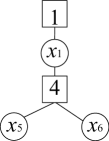
${\mathbf{X}}^{l}_{(1,1)}:=\{x_{1}x_{5}x_{6}:$ $x_{1}x_{5}x_{6}=000,011,101,110\}$

Figure 2: Illustrations of ${\mathcal{N}}^{2l}_{(1,1)}$ and ${\mathbf{X}}^{l}_{(1,1)}$, $l=2$.

• ${\mathcal{N}}^{2l}_{(i,j)}$ denotes the tree-like subset of the graph $G=({\mathcal{V}},{\mathcal{E}})$ with root edge $(i,j)$ and depth $2(l-1)$, named as the supporting tree. A formal definition is: ${\mathcal{N}}^{2l}_{(i,j)}$ is the subgraph induced by ${\mathcal{V}}^{2l}_{(i,j)}$, where

  $${\mathcal{V}}^{2l}_{(i,j)}:=\{v\in{\mathcal{V}}:d(v,i)=d(v,j)-1\in[0,2(l-1)]\},$$ (3)

  where $d(v,i)$ is the shortest distance between node $v$ and variable node $i$. In other words, ${\mathcal{N}}^{2l}_{(i,j)}$ is the depth $2(l-1)$ tree spanned from edge $(i,j)$. Let $\left|{\mathcal{N}}^{2l}_{(i,j)}\right|_{V}$ denote the number of variable nodes in ${\mathcal{N}}^{2l}_{(i,j)}$ (including variable node $i$). $\left|{\mathcal{N}}^{2l}_{(i,j)}\right|_{C}$ denotes the number of check nodes in ${\mathcal{N}}^{2l}_{(i,j)}$ (check node $j$ is excluded by definition).

• ${\mathbf{X}}=\left\{{\mathbf{x}}\in\{0,1\}^{n}:{\mathbf{A}}{\mathbf{x}}={\mathbf{0}}\right\}$ denotes the set of all valid codewords, and the information source selects each codeword equiprobably from $\mathbf{X}$.

• ${\mathbf{x}}|_{i}$ and ${\mathbf{x}}|_{{\mathcal{N}}^{2l}_{(i,j)}}$ are the projections of codeword ${\mathbf{x}}\in{\mathbf{X}}$ on bit $i$ and on the variable nodes in the supporting tree ${\mathcal{N}}^{2l}_{(i,j)}$, respectively.

• ${\mathbf{X}}^{l}_{(i,j)}$ denotes the set of all strings of length $\left|{\mathcal{N}}^{2l}_{(i,j)}\right|_{V}$ satisfying the $\left|{\mathcal{N}}^{2l}_{(i,j)}\right|_{C}$ check node constraints in ${\mathcal{N}}^{2l}_{(i,j)}$. ${\mathbf{x}}^{l}$ denotes any element of ${\mathbf{X}}^{l}_{(i,j)}$ (the subscript $(i,j)$ is omitted if there is no ambiguity). The connection between ${\mathbf{X}}$, the valid codewords, and ${\mathbf{X}}^{l}_{(i,j)}$, the tree-satisfying strings, will be clear in the following remark and in Definition 1.

• For any set of codewords (or strings) ${\mathbf{W}}$, the average operator $\langle\cdot\rangle_{\mathbf{W}}$ is defined as:

  $$\left\langle g({\mathbf{x}})\right\rangle_{\mathbf{W}}=\frac{1}{|{\mathbf{W}}|}\sum_{{\mathbf{x}}\in{\mathbf{W}}}g({\mathbf{x}}).$$

• With a slight abuse of notation for $P^{(l)}_{(i,j)}(x)$, we define

  $$P_{(i,j)}^{(l)}(x) := \left\langle P_{(i,j)}^{(l)}({\mathbf{x}})\right\rangle_{\{{\mathbf{x}}\in{\mathbf{X}}:{\mathbf{x}}|_{i}=x\}}$$

  $$P_{(i,j)}^{(l)}({\mathbf{x}}^{l}) := \left\langle P_{(i,j)}^{(l)}({\mathbf{x}})\right\rangle_{\{{\mathbf{x}}\in{\mathbf{X}}:{\mathbf{x}}|_{{\mathcal{N}}^{2l}_{(i,j)}}={\mathbf{x}}^{l}\}}.$$

  Namely, $P_{(i,j)}^{(l)}(x)$ and $P_{(i,j)}^{(l)}({\mathbf{x}}^{l})$ denote the density averaged over all compatible codewords with projections being $x$ and ${\mathbf{x}}^{l}$, respectively.

Remark: For any tree-satisfying string ${\mathbf{x}}^{l}\in{\mathbf{X}}^{l}_{(i,j)}$, there may or may not be a codeword $\mathbf{x}$ with projection ${\mathbf{x}}|_{{\mathcal{N}}^{2l}_{(i,j)}}={\mathbf{x}}^{l}$, since the codeword $\mathbf{x}$ must satisfy all check nodes, but the string ${\mathbf{x}}^{l}$ needs to satisfy only $\left|{\mathcal{N}}^{2l}_{(i,j)}\right|_{C}$ constraints. Those check nodes outside ${\mathcal{N}}^{2l}_{(i,j)}$ may limit the projected space ${\mathbf{X}}|_{{\mathcal{N}}^{2l}_{(i,j)}}$ to a strict subset of ${\mathbf{X}}^{l}_{(i,j)}$. For example, the second row of ${\mathbf{A}x}={\mathbf{0}}$ in Fig. 1 implies $x_{6}=0$. Therefore two of the four elements of ${\mathbf{X}}^{l}_{(1,1)}$ in Fig. 2 are invalid/impossible projections of $\mathbf{x}\in\mathbf{X}$ on ${\mathcal{N}}^{2l}_{(1,1)}$. Thus ${\mathbf{X}}|_{{\mathcal{N}}^{2l}_{(1,1)}}$ is a proper subset of ${\mathbf{X}}^{l}_{(1,1)}$.

To capture this phenomenon, we introduce the notion of a perfectly projected ${\mathcal{N}}^{2l}_{(i,j)}$.

Definition 1 (Perfectly Projected ${\mathcal{N}}^{2l}_{(i,j)}$)

The supporting tree ${\mathcal{N}}^{2l}_{(i,j)}$ is perfectly projected, if for any ${\mathbf{x}}^{l}\in{\mathbf{X}}^{l}_{(i,j)}$,

$$\frac{\left|\{{\mathbf{x}}\in{\mathbf{X}}:{\mathbf{x}}|_{{\mathcal{N}}^{2l}_{(i,j)}}={\mathbf{x}}^{l}\}\right|}{|{\mathbf{X}}|}=\frac{1}{\left|{\mathbf{X}}^{l}_{(i,j)}\right|}.$$ (4)

That is, if we choose $\mathbf{x}\in\mathbf{X}$ equiprobably, ${\mathbf{x}}|_{{\mathcal{N}}^{2l}_{(i,j)}}$ will appear uniformly among all elements in ${\mathbf{x}}^{l}\in{\mathbf{X}}^{l}_{(i,j)}$. Thus by looking only at the projections on ${\mathcal{N}}^{2l}_{(i,j)}$, it is as if we are choosing ${\mathbf{x}}^{l}$ from ${\mathbf{X}}^{l}_{(i,j)}$ equiprobably and there are only $\left|{\mathcal{N}}^{2l}_{(i,j)}\right|_{C}$ check node constraints and no others.

The example in Figs. 1 and 2 is obviously not perfectly projected.

Since the message emitted from node $i$ to $j$ in the $l$-th iteration depends only on the received signals of the supporting tree, $\mathbf{y}|_{{\mathcal{N}}^{2l}_{(i,j)}}$, the codeword-dependent $P_{(i,j)}^{(l)}({\mathbf{x}})$ actually depends only on the projection ${\mathbf{x}}|_{{\mathcal{N}}^{2l}_{(i,j)}}$, not on the entire codeword $\mathbf{x}$. That is

$$P_{(i,j)}^{(l)}({\mathbf{x}})=P_{(i,j)}^{(l)}({\mathbf{x}}|_{{\mathcal{N}}^{2l}_{(i,j)}}).$$ (5)

An immediate implication of ${\mathcal{N}}^{2l}_{(i,j)}$ being a perfect projection and (5) is

$$P_{(i,j)}^{(l)}(x) := \left\langle P_{(i,j)}^{(l)}({\mathbf{x}})\right\rangle_{\{{\mathbf{x}}\in{\mathbf{X}}:{\mathbf{x}}|_{i}=x\}}$$ (6)

$$= \frac{1}{\left|\{{\mathbf{x}}\in{\mathbf{X}}:{\mathbf{x}}|_{i}=x\}\right|}\sum_{\{{\mathbf{x}}\in{\mathbf{X}}:{\mathbf{x}}|_{i}=x\}}P_{(i,j)}^{(l)}({\mathbf{x}})$$

$$= \frac{1}{|\{{\mathbf{x}}\in{\mathbf{X}}:{\mathbf{x}}|_{i}=x\}|}$$

$$~{}\cdot\left|\{{\mathbf{x}}\in{\mathbf{X}}:{\mathbf{x}}|_{{\mathcal{N}}^{2l}_{(i,j)}}={\mathbf{x}}^{l},{\mathbf{x}}^{l}|_{i}=x\}\right|$$

$$~{}\cdot\sum_{\{{\mathbf{x}}^{l}\in{\mathbf{X}}^{l}_{(i,j)},{\mathbf{x}}^{l}|_{i}=x\}}P_{(i,j)}^{(l)}({\mathbf{x}}^{l})$$

$$= \left\langle P_{(i,j)}^{(l)}({\mathbf{x}}^{l})\right\rangle_{\{{\mathbf{x}}^{l}\in{\mathbf{X}}^{l}_{(i,j)}:{\mathbf{x}}^{l}|_{i}=x\}}.$$

Because of these two useful properties, (5) and (6), throughout this subsection we assume that ${\mathcal{N}}^{2l}_{(i,j)}$ is perfectly projected. The convergence of ${\mathcal{N}}^{2l}_{(i,j)}$ to a perfect projection in probability is dealt with in Section IV. We will have all the preliminaries necessary for deriving the new density evolution after introducing the following self-explanatory lemma.

Lemma 1 (Linearity of Density Transformation)

For any random variable $A$ with distribution $P_{A}$, if $g:A\mapsto g(A)$ is measurable, then $B=g(A)$ is a random variable with distribution $P_{B}=T_{g}(P_{A}):=P_{A}\circ g^{-1}$. Furthermore, the density transformation $T_{g}$ is linear. I.e. if $P_{B}=T_{g}(P_{A})$ and $Q_{B}=T_{g}(Q_{A})$, then $\alpha P_{B}+(1-\alpha)Q_{B}=T_{g}(\alpha P_{A}+(1-\alpha)Q_{A})$, $\forall\alpha\in[0,1]$.

III-B New Formula

In the $l$-th iteration, the probability of sending an incorrect message (averaged over all possible codewords) from variable node $i_{0}$ to check node $j_{0}$ is

$$p_{e}^{(l)}(i_{0},j_{0}) = \frac{1}{|{\mathbf{X}}|}\left(\sum_{\{{\mathbf{x}}\in{\mathbf{X}}:{\mathbf{x}}|_{i_{0}}=0\}}\int_{m=-\infty}^{0}P^{(l)}_{(i_{0},j_{0})}({\mathbf{x}})(dm)\right.$$ (7)

$$~{}~{}~{}~{}~{}~{}+\left.\sum_{\{{\mathbf{x}}\in{\mathbf{X}}:{\mathbf{x}}|_{i_{0}}=1\}}\int_{m=0}^{\infty}P^{(l)}_{(i_{0},j_{0})}({\mathbf{x}})(dm)\right)$$

$$= \frac{1}{2}\left(\int_{m=-\infty}^{0}P^{(l)}_{(i_{0},j_{0})}(0)(dm)\right.$$

$$~{}~{}~{}~{}+\left.\int_{m=0}^{\infty}P^{(l)}_{(i_{0},j_{0})}(1)(dm)\right).$$

Motivated by (7), we concentrate on finding an iterative formula for the density pair $P^{(l)}_{(i_{0},j_{0})}(0)$ and $P^{(l)}_{(i_{0},j_{0})}(1)$. Throughout this section, we also assume ${\mathcal{N}}^{2l}_{(i_{0},j_{0})}$ is tree-like (cycle-free) and perfectly projected.

Let $1_{\{\cdot\}}$ denote the indicator function. By an auxiliary function $\gamma(m)$:

$$\gamma(m) := \left(1_{\{m\leq 0\}},\ln\coth\left|\frac{m}{2}\right|\right),$$ (8)

and letting the domain of the first coordinate of $\gamma(m)$ be $\mathop{\sf GF}\limits(2)$, Eq. (2) for $\Psi_{c}$ can be written as

$$\Psi_{c}(m_{1},\cdots,m_{d_{c}-1}) = \gamma^{-1}\left(\sum_{v=1}^{d_{c}-1}\gamma(m_{v})\right).$$ (9)

By (1), (9), and the independence among the input messages, the classical density evolution for belief propagation algorithms (Eq. (9) in [23]) is as follows.

$$P_{(i_{0},j_{0})}^{(l)}({\mathbf{x}}) = P_{(i_{0},j_{0})}^{(0)}({\mathbf{x}})\otimes\left(\bigotimes_{c=1}^{d_{v}-1}Q_{(j_{i_{0},c},i_{0})}^{(l-1)}({\mathbf{x}})\right)$$ (10)

$$Q_{(j_{i_{0},c},i_{0})}^{(l-1)}({\mathbf{x}}) = \Gamma^{-1}\left(\bigotimes_{v=1}^{d_{c}-1}\Gamma\left(P_{(i_{j,v},j_{i_{0},c})}^{(l-1)}({\mathbf{x}})\right)\right),$$ (11)

where $\otimes$ denotes the convolution operator on probability density functions, which can be implemented efficiently using the Fourier transform. $\Gamma:=T_{\gamma}$ is the density transformation functional based on $\gamma$, defined in Lemma 1. Fig. 3 illustrates many helpful quantities used in (10), (11), and throughout this section.

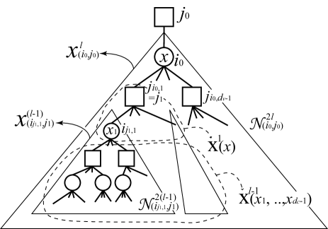
Figure 3: Illustrations of various quantities used in Section III.

By (5), (10), and the perfect projection assumption, we have

$$P_{(i_{0},j_{0})}^{(l)}({\mathbf{x}}^{l})=P_{(i_{0},j_{0})}^{(0)}({\mathbf{x}}|_{i_{0}})\otimes\left(\bigotimes_{c=1}^{d_{v}-1}Q_{(j_{i_{0},c},i_{0})}^{(l-1)}({\mathbf{x}}^{l})\right).$$ (12)

Further simplification can be made such that

$$P_{(i_{0},j_{0})}^{(l)}(x)$$

$$\stackrel{{\scriptstyle(a)}}{{=}} \left\langle P_{(i_{0},j_{0})}^{(l)}({\mathbf{x}}^{l})\right\rangle_{\{{\mathbf{x}}^{l}:{\mathbf{x}}^{l}|_{i_{0}}=x\}}$$

$$\stackrel{{\scriptstyle(b)}}{{=}} \left\langle P_{(i_{0},j_{0})}^{(0)}(x)\otimes\left(\bigotimes_{c=1}^{d_{v}-1}Q_{(j_{i_{0},c},i_{0})}^{(l-1)}({\mathbf{x}}^{l})\right)\right\rangle_{\{{\mathbf{x}}^{l}:{\mathbf{x}}^{l}|_{i_{0}}=x\}}$$

$$\stackrel{{\scriptstyle(c)}}{{=}} P_{(i_{0},j_{0})}^{(0)}(x)\otimes\left\langle\bigotimes_{c=1}^{d_{v}-1}Q_{(j_{i_{0},c},i_{0})}^{(l-1)}({\mathbf{x}}^{l})\right\rangle_{\{{\mathbf{x}}^{l}:{\mathbf{x}}^{l}|_{i_{0}}=x\}}$$

$$\stackrel{{\scriptstyle(d)}}{{=}} P_{(i_{0},j_{0})}^{(0)}(x)\otimes\left(\bigotimes_{c=1}^{d_{v}-1}\left\langle Q_{(j_{i_{0},c},i_{0})}^{(l-1)}({\mathbf{x}}^{l})\right\rangle_{\{{\mathbf{x}}^{l}:{\mathbf{x}}^{l}|_{i_{0}}=x\}}\right)$$

$$\stackrel{{\scriptstyle(e)}}{{=}} P_{(i_{0},j_{0})}^{(0)}(x)\otimes\left(\left\langle Q_{(j_{i_{0},1},i_{0})}^{(l-1)}({\mathbf{x}}^{l})\right\rangle_{\{{\mathbf{x}}^{l}:{\mathbf{x}}^{l}|_{i_{0}}=x\}}\right)^{\otimes(d_{v}-1)},$$

(13)

where (a) follows from (6), (b) follows from (12), and (c) follows from the linearity of convolutions. The fact that the sub-trees generated by edges $(j_{i_{0},c},i_{0})$ are completely disjoint implies that, by the perfect projection assumption on ${\mathcal{N}}^{2l}_{(i_{0},j_{0})}$, the distributions of strings on different sub-trees are independent. As a result, the average of the convolutional products (over these strings) equals the convolution of the averaged distributions, yielding (d). Finally (e) follows from the fact that the distributions of messages from different subtrees are identical according to the perfect projection assumption.

To simplify $\left\langle Q_{(j_{i_{0},1},i_{0})}^{(l-1)}({\mathbf{x}}^{l})\right\rangle_{\{{\mathbf{x}}^{l}:{\mathbf{x}}^{l}|_{i_{0}}=x\}}$, we need to define some new notation. We use $j_{1}$ to represent $j_{i_{0},1}$ for simplicity. Denote by $\left\{{\mathcal{N}}^{2(l-1)}_{(i_{j_{1},v},j_{1})}\right\}_{v\in[1,d_{c}-1]}$ the collection of all $d_{c}-1$ subtrees rooted at $(i_{j_{1},v},j_{1})$, $v\in[1,d_{c}-1]$, and by ${\mathbf{X}}^{l-1}_{(i_{j_{1},v},j_{1})}$ the strings compatible to ${\mathcal{N}}^{2(l-1)}_{(i_{j_{1},v},j_{1})}$. We can then consider

$${\mathbf{X}}^{1}(x)=\left\{(x_{1},\cdots,x_{d_{c}-1}):\left(\sum_{v=1}^{d_{c}-1}x_{v}\right)+x=0\right\}$$

containing the strings satisfying parity check constraint $j_{1}$ given $x_{i_{0}}=x$, and

$${\mathbf{X}}^{l-1}(x_{1},\cdots,x_{d_{c}-1})$$

$$:= \left\{({\mathbf{x}}^{l-1}_{(i_{j_{1},1},j_{1})},\cdots,{\mathbf{x}}^{l-1}_{(i_{j_{1},d_{c}-1},j_{1})}):\right.$$

$$~{}~{}~{}~{}~{}~{}~{}~{}\left.{\mathbf{x}}^{l-1}_{(i_{j_{1},1},j_{1})}|_{i_{j_{1},1}}=x_{1},\cdots,\right.$$

$$~{}~{}~{}~{}~{}~{}~{}~{}\left.{\mathbf{x}}^{l-1}_{(i_{j_{1},d_{c}-1},j_{1})}|_{i_{j_{1},d_{c}-1}}=x_{d_{c}-1}\right\}$$

is the collection of the concatenations of substrings, in which the leading symbols of the substrings are $(x_{1},\cdots,x_{d_{c}-1})$. All these quantities are illustrated in Fig. 3.

Note the following two properties: (i) For any $v$, the message $m_{v}$ from variable $i_{j_{1},v}$ to check node $j_{1}$ depends only on ${\mathbf{x}}^{l-1}_{(i_{j_{1},v},j_{1})}$; and (ii) With the leading symbols $\{x_{v}\}_{v\in[1,d_{c}-1]}$ fixed and the perfect projection assumption, the projection on the strings $\left\{{\mathbf{x}}^{l-1}_{(i_{j_{1},v},j_{1})}\right\}_{v\in[1,d_{c}-1]}$ are independent, and thus the averaged convolution of densities is equal to the convolution of the averaged densities. By repeatedly applying Lemma 1 and the above two properties, we have

$$\left\langle Q_{(j_{i_{0},1},i_{0})}^{(l-1)}({\mathbf{x}}^{l})\right\rangle_{\{{\mathbf{x}}^{l}:{\mathbf{x}}^{l}|_{i_{0}}=x\}}$$

$$=\left\langle\Gamma^{-1}\left(\bigotimes_{v=1}^{d_{c}-1}\Gamma\left(P_{(i_{j,v},j_{i_{0},c})}^{(l-1)}({\mathbf{x}}^{l})\right)\right)\right\rangle_{\{{\mathbf{x}}^{l}:{\mathbf{x}}^{l}|_{i_{0}}=x\}}$$

$$=\left\langle\Gamma^{-1}\left(\bigotimes_{v=1}^{d_{c}-1}\Gamma\left(P_{(i_{j,v},j_{i_{0},c})}^{(l-1)}({\mathbf{x}}^{l-1}_{(i_{j_{1},v},j_{1})})\right)\right)\right\rangle_{\{{\mathbf{x}}^{l}:{\mathbf{x}}^{l}|_{i_{0}}=x\}}$$

$$=\Gamma^{-1}\left(\frac{1}{2^{d_{c}-2}}\sum_{{\mathbf{x}}^{1}\in{\mathbf{X}}^{1}(x)}\right.$$

$$\hskip 42.67912pt\left.\left\langle\bigotimes_{v=1}^{d_{c}-1}\Gamma\left(P_{(i_{j,v},j_{i_{0},c})}^{(l-1)}({\mathbf{x}}^{l-1}_{(i_{j_{1},v},j_{1})})\right)\right\rangle_{{\mathbf{X}}^{l-1}({\mathbf{x}}^{1})}\right)$$

$$=\Gamma^{-1}\left(\frac{1}{2^{d_{c}-2}}\sum_{{\mathbf{x}}^{1}\in{\mathbf{X}}^{1}(x)}\bigotimes_{v=1}^{d_{c}-1}\right.$$

$$\hskip 56.9055pt\left.\Gamma\left(\left\langle P_{(i_{j,v},j_{i_{0},c})}^{(l-1)}({\mathbf{x}}^{l-1}_{(i_{j_{1},v},j_{1})})\right\rangle_{{\mathbf{X}}^{l-1}({\mathbf{x}}^{1})}\right)\right)$$

$$=\Gamma^{-1}\left(\frac{1}{2^{d_{c}-2}}\sum_{{\mathbf{x}}^{1}\in{\mathbf{X}}^{1}(x)}\bigotimes_{v=1}^{d_{c}-1}\Gamma\left(P_{(i_{j,v},j_{i_{0},c})}^{(l-1)}(x_{v})\right)\right)$$ (14)

By (13), (14), and dropping the subscripts during the density evolution, a new density evolution formula for $P^{(l)}(x)$, $\forall x=0,1$, is as follows.

$$P^{(l)}(x) = P^{(0)}(x)\otimes\left(Q^{(l-1)}(x)\right)^{\otimes(d_{v}-1)}$$

$$Q^{(l-1)}(x) = \Gamma^{-1}\left(\frac{1}{2^{d_{c}-2}}\sum_{{\mathbf{x}}^{1}\in{\mathbf{X}}^{1}(x)}\bigotimes_{v=1}^{d_{c}-1}\Gamma\left(P^{(l-1)}(x_{v})\right)\right).$$

With the help of the linearity of distribution transformations and convolutions, the above can be further simplified and the desired efficient iterative formulae become:

$$P^{(l)}(x) = P^{(0)}(x)\otimes\left(Q^{(l-1)}(x)\right)^{\otimes(d_{v}-1)}$$

$$Q^{(l-1)}(x) = \Gamma^{-1}\left(\left(\Gamma\left(\frac{P^{(l-1)}(0)+P^{(l-1)}(1)}{2}\right)\right)^{\otimes(d_{c}-1)}\right.$$

$$\left.+(-1)^{x}\left(\Gamma\left(\frac{P^{(l-1)}(0)-P^{(l-1)}(1)}{2}\right)\right)^{\otimes(d_{c}-1)}\right).$$

The above formula can be easily generalized to the irregular code ensembles ${\mathcal{C}}^{n}(\lambda,\rho)$:

$$P^{(l)}(x) = P^{(0)}(x)\otimes\lambda\left(Q^{(l-1)}(x)\right)$$

$$Q^{(l-1)}(x) = \Gamma^{-1}\left(\rho\left(\Gamma\left(\frac{P^{(l-1)}(0)+P^{(l-1)}(1)}{2}\right)\right)\right.$$

$$\left.+(-1)^{x}\rho\left(\Gamma\left(\frac{P^{(l-1)}(0)-P^{(l-1)}(1)}{2}\right)\right)\right),$$

(15)

which has the same complexity as the classical density evolution for symmetric channels.

Remark: The above derivation relies heavily on the perfect projection assumption, which guarantees that uniformly averaging over all codewords is equivalent to uniformly averaging over the tree-satisfying strings. Since the tree-satisfying strings are well-structured and symmetric, we are on solid ground to move the average inside the classical density evolution formula.

IV Density Evolution: Fundamental Theorems

As stated in Section III, the tree-like until depth $2l$ and the prefect projection assumptions are critical in our analysis. The use of codeword ensembles rather than fixed codes facilitates the analysis but its relationship to fixed codes needs to be explored. We restate two necessary theorems from [13], and give a novel perfect projection convergence theorem, which is essential to our new density evolution method. With these theorems, a concrete theoretical foundation will be established.

Theorem 1 (Convergence to the Cycle-Free Case, [13])

Fix $l$, $i_{0}$, and $j_{0}$. For any $(d_{v},d_{c})$, there exists a constant $\alpha>0$, such that for all $n\in{\mathbb{N}}$, the code ensemble ${\mathcal{C}}^{n}(d_{v},d_{c})$ satisfies

$${\mathsf{P}}\left(\mbox{${\mathcal{N}}^{2l}_{(i_{0},j_{0})}$ is cycle-free}\right)\geq 1-\alpha\left(\frac{\{(d_{v}-1)(d_{c}-1)\}^{2l}}{n}\right),$$

where ${\mathcal{N}}^{2l}_{(i_{0},j_{0})}$ is the support tree as defined by (3).

Theorem 2 (Convergence to Perfect Projection in Prob.)

Fix $l,i_{0}$, and $j_{0}$. For any regular, bipartite, equiprobable graph ensemble ${\mathcal{C}}^{n}(d_{v},d_{c})$, we have

$${\mathsf{P}}\left(\mbox{${\mathcal{N}}^{2l}_{(i_{0},j_{0})}$ is perfectly projected}\right)=1-{\mathcal{O}}(n^{-0.1}).$$

Remark: The above two theorems focus only on the properties of equiprobable regular bipartite graph ensembles, and are independent of the channel type of interest.

Theorem 3 (Concentration to the Expectation, [13])

With fixed transmitted codeword $\mathbf{x}$, let $Z$ denote the number of wrong messages (those $m$’s such that $m(-1)^{x}<0$). There exists a constant $\beta>0$ such that for any $\epsilon>0$, over the code ensemble ${\mathcal{C}}^{n}(d_{v},d_{c})$ and the channel realizations $\mathbf{y}$, we have

$${\mathsf{P}}\left(\left|\frac{Z-{\mathsf{E}}\{Z\}}{nd_{v}}\right|>\frac{\epsilon}{2}\right)\leq 2e^{-\beta\epsilon^{2}n}.$$ (16)

Furthermore, $\beta$ is independent of $f_{{\mathbf{y}}|{\mathbf{x}}}({\mathbf{y}}|{\mathbf{x}})$, and thus is independent of $\mathbf{x}$.

Theorem 3 can easily be generalized to symbol-dependent channels in the following corollary.

Corollary 1

Over the equiprobable codebook $\mathbf{X}$, the code ensemble ${\mathcal{C}}^{n}(d_{v},d_{c})$, and channel realizations $\mathbf{y}$, (16) still holds.

Proof:

Since the constant $\beta$ in Theorem 3 is independent of the transmitted codeword $\mathbf{x}$, after averaging over the equiprobable codebook $\mathbf{X}$, the inequality still holds. That is,

$${\mathsf{P}}\left(\left|\frac{Z-{\mathsf{E}}\{Z\}}{nd_{v}}\right|>\frac{\epsilon}{2}\right)={\mathsf{E}}_{\mathbf{x}}\left\{{\mathsf{P}}\left(\left|\frac{Z-{\mathsf{E}}\{Z\}}{nd_{v}}\right|>\left.\frac{\epsilon}{2}\right|{\mathbf{x}}\right)\right\}$$

$$\leq{\mathsf{E}}_{\mathbf{x}}\left\{2e^{-\beta\epsilon^{2}n}\right\}=2e^{-\beta\epsilon^{2}n}.$$

∎

Now we have all the prerequisite of proving the theoretical foundation of our codeword-averaged density evolution.

Theorem 4 (Validity of Codeword-Averaged DE)

Consider any regular, bipartite, equiprobable graph ensemble ${\mathcal{C}}^{n}(d_{v},d_{c})$ with fixed $l$, $i_{0}$, and $j_{0}$. $p_{e}^{(l)}(i_{0},j_{0})$ is derived from (7) and the codeword-averaged density evolution after $l$ iterations. The probability over equiprobable codebook $\mathbf{X}$, the code ensemble ${\mathcal{C}}^{n}(d_{v},d_{c})$, and the channel realizations $\mathbf{y}$, satisfies

$${\mathsf{P}}\left(\left|\frac{Z}{nd_{v}}-p_{e}^{(l)}(i_{0},j_{0})\right|>\epsilon\right)=e^{-\epsilon^{2}{\mathcal{O}}(n)},\forall\epsilon>0.$$

Proof:

We note that $\frac{Z}{nd_{v}}$ is bounded between 0 and 1. By observing that

$$\left(\frac{Z}{nd_{v}}\right)1\{\mbox{${\mathcal{N}}^{2l}_{(i_{0},j_{0})}$ is cycle-free and perfectly projected}\}$$

$$\leq\left(\frac{Z}{nd_{v}}\right)$$

$$\leq\left(\frac{Z}{nd_{v}}-1\right)1\{\mbox{${\mathcal{N}}^{2l}_{(i_{0},j_{0})}$ is cycle-free and perfectly projected}\}$$

$$~{}~{}~{}~{}~{}+1,$$

and using Theorems 1 and 2, we have $\lim_{n\rightarrow\infty}{{\mathsf{E}}}\left\{\frac{Z}{nd_{v}}\right\}=p_{e}^{(l)}(i_{0},j_{0})$. Then by Corollary 5, the proof is complete. ∎

The proof of Theorem 2 will be included in Appendix A

V Monotonicity, Symmetry, & Stability

In this section, we prove the monotonicity, symmetry, and stability of our codeword-averaged density evolution method on belief propagation algorithms. Since the codeword-averaged density evolution reduces to the traditional one when the channel of interest is symmetric, the following theorems also reduce to those (in [23] and [13]) for symmetric channels.

V-A Monotonicity

Proposition 1 (Monotonicity with Respect to $l$)

Let $p_{e}^{(l)}$ denote the bit error probability of the codeword-averaged density evolution defined in (7). Then $p_{e}^{(l+1)}\leq p_{e}^{(l)}$, for all $l\in{\mathbb{N}}$.

Proof:

We first note that the codeword-averaged approach can be viewed as concatenating a bit-to-sequence random mapper with the observation channels, and the larger the tree-structure is, the more observation/information the decision maker has. Since the BP decoder is the optimal MAP decoder for the tree structure of interest, the larger the tree is, the smaller the error probability will be. The proof is thus complete. ∎

Proposition 2 (Monotonicity w.r.t. Degraded Channels)

Let $f(y|x)$ and $g(y|x)$ denote two different channel models, such that $g(y|x)$ is degraded with respect to (w.r.t.) $f(y|x)$. The corresponding decoding error probabilities, $p_{e,f}^{(l)}$ and $p_{e,g}^{(l)}$, are defined in (7). Then for any fixed $l$, we have $p_{e,f}^{(l)}\leq p_{e,g}^{(l)}$.

Proof:

By taking the same point of view that the codeword-averaged approach is a concatenation of a bit-to-sequence random mapper with the observation channels, this theorem can be easily proved by the channel degradation argument. ∎

V-B Symmetry

We will now show that even though the evolved density is derived from non-symmetric channels, there are still some symmetry properties inherent in the symmetric structure of belief propagation algorithms. We define the symmetric distribution pair as follows.

Definition 2 (Symmetric Distribution Pairs)

Two probability measures ${{\mathsf{P}}}$ and ${\mathsf{Q}}$ are a symmetric pair if for any integrable function $h$, we have

$$\int h(m)d{{\mathsf{P}}}(m) =\int{e^{-m}h(-m)d{\mathsf{Q}}(m)}.$$

A distribution ${{\mathsf{P}}}_{s}$ is self-symmetric if $({{\mathsf{P}}}_{s},{{\mathsf{P}}}_{s})$ is a symmetric pair.

Proposition 3

Let $I(m):=-m$ be a parity reversing function, and let $P^{(l)}(0)$ and $P^{(l)}(1)$ denote the resulting density functions from the codeword-averaged density evolution. Then $P^{(l)}(0)$ and $P^{(l)}(1)\circ I^{-1}$ are a symmetric pair for all $l\in{\mathbb{N}}$.

Remark: In the symmetric channel case, $P^{(l)}(0)$ and $P^{(l)}(1)$ differ only in parity (Lemma 1, [13]). Thus, $P^{(l)}(0)=P^{(l)}(1)\circ I^{-1}$ is self-symmetric [Theorem 3 in [23]].

Proof: We note that by the equiprobable codeword distribution and the perfect projection assumption, $P^{(l)}(0)$ and $P^{(l)}(1)$ act on the random variable $m$, given by

$$m:=\ln\frac{{{\mathsf{P}}}(x=0|{\mathbf{y}}^{l})}{{{\mathsf{P}}}(x=1|{\mathbf{y}}^{l})}=\ln\frac{{{\mathsf{P}}}({\mathbf{y}}^{l}|x=0)}{{{\mathsf{P}}}({\mathbf{y}}^{l}|x=1)},$$

where ${\mathbf{y}}^{l}$ is the received signal on the subset ${\mathcal{N}}^{2l}$ and ${{\mathsf{P}}}$ is the distribution over channel realizations and equiprobable codewords. Then by a change of measure,

$$\int h(m)P^{(l)}(0)(dm)$$ (17)

$$= {{\mathsf{E}}}_{x=0}\left\{h\left(\ln\frac{{{\mathsf{P}}}({\mathbf{y}}^{l}|x=0)}{{{\mathsf{P}}}({\mathbf{y}}^{l}|x=1)}\right)\right\}$$

$$= {{\mathsf{E}}}_{x=1}\left\{\frac{{{\mathsf{P}}}({\mathbf{y}}^{l}|x=0)}{{{\mathsf{P}}}({\mathbf{y}}^{l}|x=1)}h\left(\ln\frac{{{\mathsf{P}}}({\mathbf{y}}^{l}|x=0)}{{{\mathsf{P}}}({\mathbf{y}}^{l}|x=1)}\right)\right\}$$

$$= \int e^{m}h(m)P^{(l)}(1)(dm).$$

This completes the proof.  ∎

Corollary 2

$$\langle P^{(l)}\rangle:=\frac{P^{(l)}(0)+P^{(l)}(1)\circ I^{-1}}{2}$$

is self-symmetric for all $l$, i.e. $(\langle P^{(l)}\rangle,\langle P^{(l)}\rangle)$ is a symmetric pair.

V-C Stability

Rather than looking only at the error probability $p_{e}^{(l)}$ of the evolved densities $P^{(l)}(0)$ and $P^{(l)}(1)$, we also focus on its Chernoff bound,

$$CBP^{(l)}(x):=\int e^{-\frac{(-1)^{x}m}{2}}P^{(l)}(x)(dm).$$

By letting $h(m)=e^{-\frac{m}{2}}$ and by (17), we have $CBP^{(l)}(0)=CBP^{(l)}(1)$. The averaged $\langle CBP^{(l)}\rangle$ then becomes

$$\langle CBP^{(l)}\rangle := \frac{1}{2}\left(CBP^{(l)}(0)+CBP^{(l)}(1)\right)$$ (18)

$$= CBP^{(l)}(0)=CBP^{(l)}(1)$$

$$= \int e^{\frac{-m}{2}}\langle P^{(l)}\rangle(dm).$$

We state three properties which can easily be derived from the self-symmetry of $\langle P^{(l)}\rangle$. Proofs can be found in [31, 23], and [30].

• $\langle CBP^{(l)}\rangle=\min_{s}\int e^{-s\cdot m}\langle P^{(l)}\rangle(dm)$.

• The density of $e^{-m/2}\langle P^{(l)}\rangle(dm)$ is symmetric with respect to $m=0$.

• $2p_{e}^{(l)}\leq\langle CBP^{(l)}\rangle\leq 2\sqrt{p_{e}^{(l)}(1-p_{e}^{(l)})}$. This justifies the use of $\langle CBP^{(l)}\rangle$ as our performance measure.

Thus, we consider $\langle CBP^{(l)}\rangle$, the Chernoff bound of $p_{e}^{(l)}$. With the regularity assumption that $\int_{{\mathbf{R}}}e^{sm}\langle P^{(0)}\rangle(dm)<\infty$ for all $s$ in some neighborhood of zero, we state the necessary and sufficient stability conditions as follows.

Theorem 5 (Sufficient Stability Condition)

Let $r:=\langle CBP^{(0)}\rangle=\int_{\mathbf{R}}e^{-m/2}\langle P^{(0)}\rangle(dm)$. Suppose $\lambda_{2}\rho^{\prime}(1)r<1$, and let $\epsilon^{*}$ be the smallest strictly positive root of the following equation.

$$\lambda(\rho^{\prime}(1)\epsilon)r=\epsilon.$$

If for some $l_{0}$, $\langle CBP^{(l_{0})}\rangle<\epsilon^{*}$, then

$$\langle CBP^{(l)}\rangle=\begin{cases}{{\mathcal{O}}}\left(\left(\lambda_{2}\rho^{\prime}(1)r\right)^{l}\right)&\text{if $\lambda_{2}>0$}\\ {{\mathcal{O}}}\left(e^{-{\mathcal{O}}\left((k_{\lambda}-1)^{l}\right)}\right)&\text{if $\lambda_{2}=0$}\end{cases},$$

where $k_{\lambda}=\min\{k:\lambda_{k}>0\}$. In both cases: $\lambda_{2}=0$ and $\lambda_{2}>0$, $\lim_{l\rightarrow\infty}\langle CBP^{(l)}\rangle=0$.

Corollary 3

For any noise distribution $f(y|x)$ with Bhattacharyya noise parameter $r:=\langle CBP^{(0)}\rangle$, if there is no $\epsilon\in(0,r)$ such that

$$\lambda(\rho^{\prime}(1)\epsilon)r=\epsilon,$$

then ${\mathcal{C}}(\lambda,\rho)$ will have arbitrarily small bit error rate as $n$ tends to infinity. The corresponding $r$ can serve as an inner bound of the achievable region for general non-symmetric memoryless channels. Further discussion of finite dimensional bounds on the achievable region can be found in [30].

Theorem 6 (Necessary Stability Condition)

Let $r:=\langle CBP^{(0)}\rangle$. If $\lambda_{2}\rho^{\prime}(1)r>1$, then $\lim_{l\rightarrow\infty}p^{(l)}_{e}>0$.

• Remark 1: $\langle CBP^{(0)}\rangle$ is the Bhattacharyya noise parameter and is related to the cutoff rate $R_{0}$ by $R_{0}=1-\log_{2}(1+\langle CBP^{(0)}\rangle)$. Further discussion of $\langle CBP^{(0)}\rangle$ for turbo-like and LDPC codes can be found in [25, 31, 30].

• Remark 2: The stability results are first stated in [23] without the convergence rate statement and the stability region $\epsilon^{*}$. Since we focus on general asymmetric channels (with symmetric channels as a special case), our convergence rate and stability region $\epsilon^{*}$ results also apply to the symmetric channel case. Benefitting from considering its Chernoff version, we will provide a simple proof, which did not appear in [23].

• Remark 3: $\epsilon^{*}$ can be used as a stopping criterion for the iterations of the density evolution. Moreover, $\epsilon^{*}$ is lower bounded by $\frac{1-\lambda_{2}\rho^{\prime}(1)r}{\lambda(\rho^{\prime}(1))r-\lambda_{2}\rho^{\prime}(1)r}$, which is a computationally efficient substitute for $\epsilon^{*}$.

Proof of Theorem 5: We define the Chernoff bound of the density of the messages emitting from check nodes, $CBQ^{(l)}(x)$, in a fashion similar to $CBP^{(l)}(x)$:

$$CBQ^{(l)}(x):=\int e^{-\frac{(-1)^{x}m}{2}}Q^{(l)}(x)(dm).$$

First consider the case in which $d_{c}=3$. We then have

$$\Psi_{c}(m_{1},m_{2}) = \ln\left(\frac{1+\tanh\frac{m_{1}}{2}\tanh\frac{m_{2}}{2}}{1-\tanh\frac{m_{1}}{2}\tanh\frac{m_{2}}{2}}\right)$$

$$= \ln\frac{e^{m_{1}}e^{m_{2}}+1}{e^{m_{1}}+e^{m_{2}}}.$$

To simplify the analysis, we assume the all-zero codeword is transmitted and then generalize the results to non-zero codewords. Suppose the distributions of $m_{1}$ and $m_{2}$ are $P^{(l)}_{1}(0)$ and $P^{(l)}_{2}(0)$, respectively. The $CBQ^{(l)}(0)$ becomes

$$CBQ^{(l)}(0)$$ (19)

$$= \int e^{-\frac{\Psi_{c}(m_{1},m_{2})}{2}}P^{(l)}_{1}(0)(dm_{1})\times P^{(l)}_{2}(0)(dm_{2})$$

$$= \int\sqrt{\frac{e^{m_{1}}+e^{m_{2}}}{e^{m_{1}}e^{m_{2}}+1}}P^{(l)}_{1}(0)(dm_{1})\times P^{(l)}_{2}(0)(dm_{2})$$

$$\leq \int\sqrt{e^{m_{1}}+e^{m_{2}}}P^{(l)}_{1}(0)(dm_{1})\times P^{(l)}_{2}(0)(dm_{2})$$

$${\leq} \int\sqrt{e^{m_{1}}}+\sqrt{e^{m_{2}}}P^{(l)}_{1}(0)(dm_{1})\times P^{(l)}_{2}(0)(dm_{2})$$

$$= CBP^{(l)}_{1}(0)+CBP^{(l)}_{2}(0),$$

where the last inequality follows from the fact that $\forall\alpha,\beta\geq 0,\sqrt{\alpha+\beta}\leq\sqrt{\alpha}+\sqrt{\beta}$. Since any check node with $d_{c}>3$ can be viewed as the concatenation of many check nodes with $d_{c}=3$, by induction and by assuming the all-zero codeword is transmitted, we have

$$CBQ^{(l)}(0)\leq(d_{c}-1)CBP^{(l)}(0).$$ (20)

Since $CBP^{(l)}(0)=CBP^{(l)}(1)$ as in (18), the averaging over all possible codewords does not change (20). By further incorporating the check node degree polynomial $\rho$, we have

$$\forall x\in\{0,1\},~{}CBQ^{(l)}(x) \leq \sum_{k}\rho_{k}(k-1)\left\langle CBP^{(l)}\right\rangle$$

$$= \rho^{\prime}(1)\langle CBP^{(l)}\rangle.$$

By (15) and the fact that the moment generating function of the convolution equals the product of individual moment generating functions, we have

$$CBP^{(l+1)}(x) = CBP^{(0)}(x)\sum_{k}\lambda_{k}\left(CBQ^{(l)}(x)\right)^{k-1}$$

$$\leq CBP^{(0)}(x)\lambda\left(\rho^{\prime}(1)\langle CBP^{(l)}\rangle\right),$$

which is equivalent to

$$\langle CBP^{(l+1)}\rangle \leq \langle CBP^{(0)}\rangle\lambda\left(\rho^{\prime}(1)\langle CBP^{(l)}\rangle\right).$$ (21)

The sufficient stability theorem follows immediately from (21), the iterative upper bound formula.  ∎

Remark: (21) is a one-dimensional iterative bound for general asymmetric memoryless channels. In [30], this iterative upper bound will be further strengthened to:

$$\langle CBP^{(l+1)}\rangle \leq \langle CBP^{(0)}\rangle\lambda\left(1-\rho\left(1-\langle CBP^{(l)}\rangle\right)\right),$$

which is tight for BECs and holds for asymmetric channels as well.

Proof of Theorem 6: We prove this result by the erasure decomposition technique used in [23].

The erasure decomposition lemma in [23] states that, for any $l_{0}>0$, and any symmetric channel $f$ with log likelihood ratio distribution $P^{(l_{0})}$, there exists a BEC $g$ with log likelihood ratio distribution $B^{(l_{0})}$ such that $f$ is physically degraded with respect to $g$. Furthermore, $B^{(l_{0})}$ is of the following form:

$$B^{(l_{0})}=2\epsilon\delta_{0}+(1-2\epsilon)\delta_{\infty},$$

for all $\epsilon\leq p_{e}^{(l_{0})}$, where $\delta_{x}$ is the Dirac-delta measure centered at $x$. It can be easily shown that this erasure decomposition lemma holds even when $f$ corresponds to a non-symmetric channel with LLR distributions $\{P^{(l_{0})}(x)\}_{x=0,1}$ and $p_{e}^{(l_{0})}$ computed from (7).

We can then assign $B^{(l_{0})}(0):=B^{(l_{0})}$ and $B^{(l_{0})}(1):=B^{(l_{0})}\circ I^{-1}$ to distinguish the distributions for different transmitted symbols $x$.

Suppose $r\lambda_{2}\rho^{\prime}(1)>1$ and $\lim_{l\rightarrow\infty}p_{e}^{(l)}=0$. Then for any $\epsilon>0$, $\exists l_{0}>0$, such that $p_{e}^{(l_{0})}\leq\epsilon$. For simplicity, we assume $p_{e}^{(l_{0})}=\epsilon$. The physically better BEC is described as above. If during the iteration procedure (15), we replace the density $P^{(l_{0})}(x)$ with $B^{(l_{0})}(x)$, then the resulting density will be

$$P_{B}^{(l_{0}+\Delta l)}(0)$$

$$= 2\epsilon\left(\lambda_{2}\rho^{\prime}(1)\right)^{\Delta l}P^{(0)}(0)\otimes\left(\langle P^{(0)}\rangle\right)^{\otimes(\Delta l-1)}$$

$$+\left(1-2\epsilon\left(\lambda_{2}\rho^{\prime}(1)\right)^{\Delta l}\right)\delta_{\infty}+{\mathcal{O}}(\epsilon^{2})$$

$$P_{B}^{(l_{0}+\Delta l)}(1)$$

$$= 2\epsilon\left(\lambda_{2}\rho^{\prime}(1)\right)^{\Delta l}P^{(0)}(1)\otimes\left(\langle P^{(0)}\rangle\circ I^{-1}\right)^{\otimes(\Delta l-1)}$$

$$+\left(1-2\epsilon\left(\lambda_{2}\rho^{\prime}(1)\right)^{\Delta l}\right)\delta_{-\infty}+{\mathcal{O}}(\epsilon^{2}),$$

and the averaged error probability $p_{e,B}^{(l_{0}+\Delta l)}$ is

$$p_{e,B}^{(l_{0}+\Delta l)} := \int_{-\infty}^{0}\frac{P_{B}^{(l_{0}+\Delta l)}(0)+P_{B}^{(l_{0}+\Delta l)}(1)\circ I^{-1}}{2}(dm)$$

$$= {\mathcal{O}}(\epsilon^{2})+2\epsilon(\lambda_{2}\rho^{\prime}(1))^{\Delta l}\int_{-\infty}^{0}d\left(\langle P^{(0)}\rangle\right)^{\otimes\Delta l}.$$

By the fact that $r=\langle CBP^{(0)}\rangle$ is the Chernoff bound on $\int_{-\infty}^{0}d\langle P^{(0)}\rangle$, the regularity condition and the Chernoff theorem, for any $\epsilon^{\prime}>0$, there exists a large enough $\Delta l$ such that

$$\int_{-\infty}^{0}d\left(\langle P^{(0)}\rangle\right)^{\otimes\Delta l}\geq(r-\epsilon^{\prime})^{\Delta l}.$$

With a small enough $\epsilon^{\prime}$, we have $\lambda_{2}\rho^{\prime}(1)(r-\epsilon^{\prime})>1$. Thus with large enough $\Delta l$, we have

$$p_{e,B}^{(l_{0}+\Delta l)} > {\mathcal{O}}(\epsilon^{2})+2\epsilon.$$

With small enough $\epsilon$ or equivalently large enough $l_{0}$, we have

$$p_{e,B}^{(l_{0}+\Delta l)} > {\mathcal{O}}(\epsilon^{2})+2\epsilon>\epsilon=p_{e}^{(l_{0})}.$$

However, by the monotonicity with respect to physically degraded channels we have, $p_{e}^{(l_{0}+\Delta l)}\geq p_{e,B}^{(l_{0}+\Delta l)}>p_{e}^{(l_{0})}$, which contradicts the monotonicity of $p_{e}^{(l)}$ with respect to $l$. From the above reasoning, if $r\lambda_{2}\rho^{\prime}(1)>1$, then $\lim_{l\rightarrow\infty}p_{e}^{(l)}>0$, which completes the proof.  ∎

Remark: From the sufficient stability condition, for those codes with $\lambda_{2}>0$, the convergence rate is exponential in $l$, i.e. $BER=O\left((r\lambda_{2}\rho^{\prime}(1))^{l}\right)$. However the number of bits involved in the ${\mathcal{N}}^{2l}$ tree is $O\left(\left((d_{v}-1)(d_{c}-1)\right)^{l}\right)$, which is usually much faster than the reciprocal of the decrease rate of $BER=O\left((r\lambda_{2}\rho^{\prime}(1))^{l}\right)$. As a result, we conjecture that the average performance of the code ensemble with $\lambda_{2}>0$ will have bad block error probabilities. This is confirmed in Fig. 5(b) and theoretically proved for the BEC in [32]. The converse is stated and proved in the following corollary.

Corollary 4

Let ${{\mathsf{E}}}\left\{Z_{B}^{(l)}\right\}$ denote the block error probability of codeword length $n$ after $l$ iterations of the belief propagation algorithm, which is averaged over equiprobable codewords, channel realizations, and the code ensemble ${\mathcal{C}}^{n}(\lambda,\rho)$. If $\lambda_{2}=0$ and $l_{n}$ satisfying $\ln\ln n=o(l_{n})$ and $l_{n}=o(\ln n)$,

$$\lim_{n\rightarrow\infty}{{\mathsf{E}}}\left\{Z_{B}^{(l_{n})}\right\}=0.$$

Proof:

This result can be proven directly by the cycle-free convergence theorem, the super-exponential bit convergence rate with respect to $l$, and the union bound. ∎

A similar observation is also made and proved in [25], in which it is shown that the interleaving gain exponent of the block error rate is $-J+2$, where $J$ is the number of parallel constituent codes. The variable node degree $d_{v}$ is the number of parity check equations (parity check sub-codes) in which a variable bit participates. In a sense, an LDPC code is similar to $d_{v}$ parity check codes interleaved together. With $d_{v}=2$, good interleaving gain for the block error probability is not expected.

VI Simulations and Discussion

It is worth noting that for non-symmetric channels, different codewords will have different error-resisting capabilities. In this section, we consider the averaged performance. We can obtain codeword-independent performance by adding a random number to the information message before encoding and then subtracting it after decoding. This approach, however, introduces higher computational cost.

VI-A Simulation Settings

With the help of the sufficient condition of the stability theorem (Theorem 5), we can use $\epsilon^{*}$ to set a stopping criterion for the iterations of the density evolution. We use the 8-bit quantized density evolution method with $(-15,15)$ being the domain of the LLR messages. We will determine the largest thresholds such that the evolved Chernoff bound $\langle CBP^{(l)}\rangle$ hits $\epsilon^{*}$ within 100 iterations, i.e. $\langle CBP^{(100)}\rangle<\epsilon^{*}$. Better performance can be achieved by using more iterations, which, however, is of less practical interest. For example, the 500-iteration threshold of our best code for z-channels, 12B (described below), is 0.2785, compared to the 100-iteration threshold 0.2731. Five different code ensembles with rate $1/2$ are extensively simulated, including regular $(3,6)$ codes, regular $(4,8)$ codes, 12A codes, 12B codes, and 12C codes, where

• 12A: 12A is a rate-$1/2$ code ensemble found by Richardson, et al. in [23], which is the best known degree distribution optimized for the symmetric BiAWGNC, having maximum degree constraints $\max d_{v}\leq 12$ and $\max d_{c}\leq 9$. Its degree distributions are

  $$\lambda(x) = 0.24426x+0.25907x^{2}+0.01054x^{3}$$

  $$+0.05510x^{4}+0.01455x^{7}+0.01275x^{9}$$

  $$+0.40373x^{11},$$

  $$\rho(x) = 0.25475x^{6}+0.73438x^{7}+0.01087x^{8}.$$

• 12B: 12B is a rate-$1/2$ code ensemble obtained by minimizing the hitting time of $\epsilon^{*}$ in z-channels, through hill-climbing and linear programming techniques. The maximum degree constraints are also $\max d_{v}\leq 12$ and $\max d_{c}\leq 9$. The differences between 12A and 12B are (1) 12B is optimized for the z-channels with our codeword-averaged density evolution, and 12A is optimized for the symmetric BiAWGNC. (2) 12B is optimized with respect to the hitting time of $\epsilon^{*}$ (depending on $(\lambda,\rho)$) rather than a fixed small threshold. The degree distributions of 12B are

  $$\lambda(x) = 0.236809x+0.309590x^{2}+0.032789x^{3}$$

  $$+0.007116x^{4}+0.000001x^{5}+0.413695x^{11},$$

  $$\rho(x) = 0.000015x^{5}+0.464854x^{6}+0.502485x^{7}$$

  $$+0.032647x^{8}.$$

• 12C: 12C a rate-$1/2$ code ensemble similar to 12B, but with $\lambda_{2}$ being hard-wired to $0$, which is suggested by the convergence rate in the sufficient stability condition. The degree distributions of 12C are

  $$\lambda(x) = 0.861939x^{2}+0.000818x^{3}+0.000818x^{4}$$

  $$+0.000818x^{5}+0.000818x^{6}+0.000818x^{7}$$

  $$+0.000218x^{8}+0.077898x^{9}+0.055843x^{10}$$

  $$+0.000013x^{11},$$

  $$\rho(x) = 0.000814x^{4}+0.560594x^{5}+0.192771x^{6}$$

  $$+0.145207x^{7}+0.100613x^{8}.$$

Codes	BEC		BSC		Z-channels		BiAWGNC		Stability $\langle CBP\rangle$
	$\epsilon$	$\langle CBP\rangle$	$\epsilon$	$\langle CBP\rangle$	$\epsilon_{1}$	$\langle CBP\rangle$	$\sigma$	$\langle CBP\rangle$
(3,6)	0.4294	0.4294	0.0837	0.5539	0.2305	0.4828	0.8790	0.5235	–
(4,8)	0.3834	0.3834	0.0764	0.5313	0.1997	0.4497	0.8360	0.4890	–
12A	0.4682	0.4682	0.0937	0.5828	0.2710	0.5233	0.9384	0.5668	0.6060
12B	0.4753	0.4753	0.0939	0.5834	0.2731	0.5253	0.9362	0.5653	0.6247
12C	0.4354	0.4354	0.0862	0.5613	0.2356	0.4881	0.8878	0.5303	–
Sym. Info. Rate	0.5000	0.5000	0.1100	0.6258	0.2932	0.5415	0.9787	0.5933	–
Capacity	0.5000	0.5000	0.1100	0.6258	0.3035	0.5509	0.9787	0.5933	–

TABLE I: Thresholds of different codes and channels, with precision $10^{-4}$.

Four different channels are considered, including the BEC, BSC, z-channel, and BiAWGNC. Z-channels are simulated by binary non-symmetric channels with very small $\epsilon_{0}$ ($\epsilon_{0}=0.00001$) and different values of $\epsilon_{1}$. TABLE I summarizes the thresholds with precision $10^{-4}$. Thresholds are not only presented by their conventional channel parameters, but also by their Bhattacharyya noise parameters (Chernoff bounds). The column “stability” lists the maximum $r:=\langle CBP^{(0)}\rangle$ such that $r\lambda_{2}\rho^{\prime}(1)<1$, which is an upper bound on the $\langle CBP^{(0)}\rangle$ values of decodable channels. Further discussion of the relationship between $\langle CBP^{(0)}\rangle$ and the decodable threshold can be found in [30].

From TABLE I, we observe that 12A outperforms 12B in Gaussian channels (for which 12A is optimized), but 12B is superior in z-channels for which it is optimized. The above behavior promises room for improvement with codes optimized for different channels, as was also shown in [14].

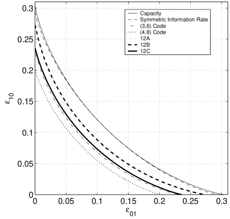
Figure 4: Asymptotic thresholds and the achievable regions of different codes in binary asymmetric channels.

Fig. 4 demonstrates the asymptotic thresholds of these codes in binary asymmetric channels (BASCs) with the curves of 12A and 12B being very close together. It is seen that 12B is slightly better when $\epsilon_{0},\epsilon_{1}\rightarrow 0$ or $\epsilon_{0}\approx\epsilon_{1}$. We notice that all the achievable regions of these codes are bounded by the symmetric mutual information rate (with a $(1/2,1/2)$ a priori distribution), which was also suggested in [16]. The difference between the symmetric mutual information rate and the capacity for non-symmetric channels is generally indistinguishable from the practical point of view. For example, in [33], it was shown that the ratio between the symmetric mutual information rate and the capacity is lower bounded by $\frac{e\ln 2}{2}\approx 0.942$. [34] further proved that the absolute difference is upper bounded by $0.011$ bit/sym. Further discussion of capacity achieving codes with non-uniform a priori distributions can be found in [35] and [29].

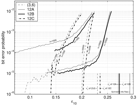
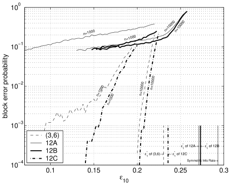
(a) Bit error rates	(b) Block error rates

Figure 5: Bit/block error rates versus $\epsilon_{1}$ with fixed $\epsilon_{0}=0.00001$. Computed thresholds for symmetric mutual information rate, (3,6), 12A, 12B, and 12C codes are $0.2932$, $0.2305$, $0.2710$, $0.2730$, and $0.2356$, respectively. $40$ iterations of belief propagation algorithms were performed. 10,000 codewords were used for the simulations.

Figs. 5(a) and 5(b) consider several fixed finite codes in z-channels. We arbitrarily select graphs from the code ensemble with codeword lengths $n=$1,000 and $n=$10,000. Then, with these graphs (codes) fixed, we find the corresponding parity matrix $\mathbf{A}$, use Gaussian elimination to find the generator matrix $\mathbf{G}$, and transmit different codewords by encoding equiprobably selected information messages. Belief propagation decoding is used with $40$ iterations for each codeword. 10,000 codewords are transmitted, and the overall bit/block error rates versus different $\epsilon_{1}$ are plotted for different code ensembles and codeword lengths. Our new density evolution predicts the waterfall region quite accurately when the bit error rates are of primary interest. Though there are still gaps between the performance of finite codes and our asymptotic thresholds, the performance gaps between different finite length codes are very well predicted by the differences between their asymptotic thresholds. From the above observations and the underpinning theorems, we see that our new density evolution is a successful generalization of the traditional one from both practical and theoretical points of view.

Fig. 5(b) exhibits the block error rate of the same 10,000-codeword simulation. The conjecture of bad block error probabilities for $\lambda_{2}>0$ codes is confirmed. Besides the conjectured bad block error probabilities, Figs. 5(a) and 5(b) also suggest that codes with $\lambda_{2}=0$ will have a better error floor compared to those with $\lambda_{2}>0$, which can be partly explained by the comparatively slow convergence speed stated in the sufficient stability condition for $\lambda_{2}>0$ codes. 12C is so far the best code we have for $\lambda_{2}=0$. However, its threshold is not as good as those of 12A and 12B. If good block error rate and low error floor are our major concerns, 12C (or other codes with $\lambda_{2}=0$) can still be competitive choices. Recent results in [36] shows that the error floor for codes with $\lambda_{2}>0$ can be lowered by carefully arranging the degree two variable nodes in the corresponding graph while keeping a similar waterfall threshold.

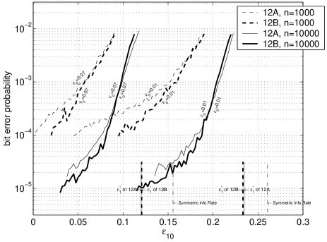
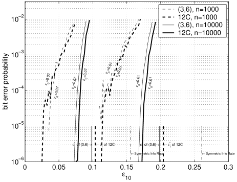
(a) 12A & 12B:	(b) 12C & regular (3,6) codes

Figure 6: Bit error rates versus $\epsilon_{1}$ for $\epsilon_{0}=0.01$ and $\epsilon_{0}=0.7$. The DE thresholds of (12A, 12B, 12C, (3,6)) are $(0.2346,0.2332,0.2039,0.1981)$ for $\epsilon_{0}=0.01$ and $(0.1202,0.1206,0.1036,0.0982)$ for $\epsilon_{0}=0.07$. $40$ iterations of belief propagation algorithms were performed. 2,000 codewords were used for the simulations.

Figs. 6(a) and 6(b) illustrate the bit error rates versus different BASC settings with 2,000 transmitted codewords. Our computed density evolution threshold is again highly correlated with the performance of finite length codes for different asymmetric channel settings.

We close this section by highlighting two applications of our results.

1. Error Floor Analysis: “The error floor” is a characteristic of iterative decoding algorithms, which is of practical importance and may not be able to be determined solely by simulations. More analytical tools are needed to find error floors for corresponding codes. Our convergence rate statements in the sufficient stability condition may shed some light on finding codes with low error floors.

2. Capacity-Approaching Codes for General Non-Standard Channels: Various very good codes (capacity-approaching) are known for standard channels, but very good codes for non-standard channels are not yet known. It is well known that one can construct capacity-approaching codes by incorporating symmetric-information-rate-approaching linear codes with the symbol mapper and demapper as an inner code [29, 35, 37]. Understanding density evolution for general memoryless channels allows us to construct such symmetric-information-rate-approaching codes (for non-symmetric memoryless channels), and thus to find capacity-approaching codes after concatenating the inner symbol mapper and demapper. It is worth noting that intersymbol interference channels are dealt with by Kavčić et al. in [16] using the coset codes approach. It will be of great help if a unified framework for non-symmetric channels with memory can be found by incorporating both coset codes and codeword averaging approaches.

VII Further Implications of Generalized Density Evolution

VII-A Typicality of Linear LDPC Codes

(a) Linear Code Ensemble versus Non-symmetric Channels

(b) Linear Code Ensemble versus Symmetrized Channels

(c) Coset Code Ensemble versus Non-symmetric Channels

Figure 7: Comparison of the approaches based on codeword averaging and the coset code ensemble.

One reason that non-symmetric channels are often overlooked is we can always transform a non-symmetric channel into a symmetric channel. Depending on different points of view, this channel-symmetrizing technique is termed the coset code argument [16] or dithering/the i.i.d. channel adapter [21], as illustrated in Figs. 7(c) and 7(b). Our generalized density evolution provides a simple way to directly analyze the linear LDPC code ensemble on non-symmetric channels, as in Fig. 7(a).

As shown in Theorems 5 and 6, the necessary and sufficient stability conditions of linear LDPC codes for non-symmetric channels, Fig. 7(a), are identical to those of the coset code ensemble, Fig. 7(c). Monte Carlo simulations based on finite-length codes ($n=10^{4}$) [21] further show that the codeword-averaged performance in Fig. 7(a) is nearly identical to the performance of Fig. 7(c) when the same encoder/decoder pair is used. The above two facts suggest a close relationship between linear codes and the coset code ensemble, and it was conjectured in [21] that the scheme in Fig. 7(a) should always have the same/similar performance as those illustrated by Fig. 7(c). This short subsection is devoted to the question whether the systems in Figs. 7(a) and 7(c) are equivalent in terms of performance. In sum, the performance of the linear code ensemble is very unlikely to be identical to that of the coset code ensemble. However, when the minimum $d_{c,min}:=\{k\in{\mathbb{N}}:\rho_{k}>0\}$ is sufficiently large, we can prove that their performance discrepancy is theoretically indistinguishable. In practice, the discrepancy for $d_{c,min}\geq 6$ is $<0.05\%$.

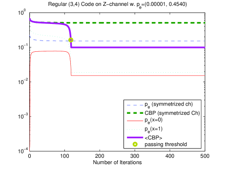
Figure 8: Density evolution for z-channels with the linear code ensemble and the coset code ensemble.

Let $P_{a.p.}^{(l)}(0):=P^{(l)}(0)$ and $P_{a.p.}^{(l)}(1):=P^{(l)}(1)\circ I^{-1}$ denote the two evolved densities with aligned parity, and similarly define $Q_{a.p.}^{(l)}(0):=Q^{(l)}(0)$ and $Q_{a.p.}^{(l)}(1):=Q^{(l)}(1)\circ I^{-1}$. Our main result in (15) can be rewritten in the following form:

$$P^{(l)}_{a.p.}(x) = P^{(0)}_{a.p.}(x)\otimes\lambda\left(Q^{(l-1)}_{a.p.}(x)\right)$$

$$Q^{(l-1)}_{a.p.}(x) = \Gamma^{-1}\left(\rho\left(\Gamma\left(\frac{P^{(l-1)}_{a.p.}(0)+P^{(l-1)}_{a.p.}(1)}{2}\right)\right)\right.$$

$$\left.+(-1)^{x}\rho\left(\Gamma\left(\frac{P^{(l-1)}_{a.p.}(0)-P^{(l-1)}_{a.p.}(1)}{2}\right)\right)\right).$$

Let $p^{(l)}_{e,linear}$ denote the corresponding bit error probability of the linear codes after $l$ iterations. For comparison, the traditional formula of density evolution for the symmetrized channel (the coset code ensemble) is as follows:

$$P^{(l)}_{coset} = P^{(0)}_{coset}\otimes\lambda\left(Q^{(l-1)}_{coset}\right)$$

$$Q^{(l-1)}_{coset} = \Gamma^{-1}\left(\rho\left(\Gamma\left(P^{(l-1)}_{coset}\right)\right)\right),$$ (24)

where $P^{(0)}_{coset}=\frac{\sum_{x=0,1}P^{(0)}_{a.p.}(x)}{2}$. Similarly, let $p^{(l)}_{e,coset}$ denote the corresponding bit error probability.

It is clear from the above formulae that when the channel of interest is symmetric, namely $P^{(0)}_{a.p.}(0)=P^{(0)}_{a.p.}(1)$, then $P^{(l)}_{coset}=P^{(l)}_{a.p.}(0)=P^{(l)}_{a.p.}(1)$ for all $l\in{\mathbb{N}}$. However, for non-symmetric channels, since the variable node iteration involves convolution of several densities given the same $x$ value, the difference between $Q^{(l-1)}_{a.p.}(0)$ and $Q^{(l-1)}_{a.p.}(1)$ will be amplified after each variable node iteration. Hence it is very unlikely that the decodable thresholds of linear codes and coset codes will be analytically identical, namely

$$\lim_{l\rightarrow\infty}p^{(l)}_{e,linear}=0\stackrel{{\scriptstyle?}}{{\Longleftrightarrow}}\lim_{l\rightarrow\infty}p^{(l)}_{e,coset}=0.$$

Fig. 8 demonstrates the traces of the evolved densities for the regular (3,4) code on z-channels. With the one-way crossover probability being 0.4540, the generalized density evolution for linear codes is able to converge within 179 iterations, while the coset code ensemble shows no convergence within 500 iterations. This demonstrates the possible performance discrepancy, though we do not have analytical results proving that the latter will not converge after further iterations. TABLE II compares the decodable thresholds such that the density evolution enters the stability region within 100 iterations. We notice that the larger $d_{c,min}$ is, the smaller the discrepancy is. This phenomenon can be characterized by the following theorem.

TABLE II: Threshold comparison $p^{*}_{1\rightarrow 0}$ of linear and coset LDPC codes on Z-channels

$(\lambda,\rho)$	$(x^{2},x^{3})$	$(x^{2},x^{5})$
Linear	0.4540	0.2305
Coset	0.4527	0.2304
$(\lambda,\rho)$	$(x^{2},0.5x^{2}+0.5x^{3})$	$(x^{2},0.5x^{4}+0.5x^{5})$
Linear	0.5888	0.2689
Coset	0.5908	0.2690

Theorem 7

Consider non-symmetric memoryless channels and a fixed pair of finite-degree polynomials $\lambda$ and $\rho$. The shifted version of the check node polynomial is denoted as $\rho_{\Delta}=x^{\Delta}\cdot\rho$ where $\Delta\in{\mathbb{N}}$. Let $P^{(l)}_{coset}$ denote the evolved density from the coset code ensemble with degrees $(\lambda,\rho_{\Delta})$, and $\langle P^{(l)}\rangle=\frac{1}{2}\sum_{x=0,1}P^{(l)}_{a.p.}(x)$ denote the averaged density from the linear code ensemble with degrees $(\lambda,\rho_{\Delta})$. For any $l_{0}\in{\mathbb{N}}$, $\lim_{\Delta\rightarrow\infty}\langle P^{(l)}\rangle\stackrel{{\scriptstyle\mathcal{D}}}{{=}}P^{(l)}_{coset}$ in distribution for all $l\leq l_{0}$, with the convergence rate for each iteration being ${\mathcal{O}}\left({\mathsf{const}}^{\Delta}\right)$ for some ${\mathsf{const}}<1$.

Corollary 5 (The Typicality Results for Z-Channels)

For any $\epsilon>0$, there exists a $\Delta\in{\mathbb{N}}$ such that

$$\left|\sup\left\{p_{1\rightarrow 0}:\lim_{l\rightarrow\infty}p^{(l)}_{e,linear}=0\right\}-\sup\left\{p_{1\rightarrow 0}:\lim_{l\rightarrow\infty}p^{(l)}_{e,coset}=0\right\}\right|$$

$$<\epsilon.$$

Namely, the asymptotic decodable thresholds of the linear and the coset code ensemble are arbitrarily close when the minimum check node degree $d_{c,min}$ is sufficiently large.

Similar corollaries can be constructed for other channel models with different types of noise parameters, e.g., the $\sigma^{*}$ in the composite BiAWGNC. A proof of Corollary 5 is found in Appendix C.

Proof of Theorem 7: Since the functionals in (LABEL:eq:dens-linear) and (24) are continuous with respect to convergence in distribution, we need only to show that $\forall l\in{\mathbb{N}}$,

$$\lim_{\Delta\rightarrow\infty}Q^{(l-1)}_{a.p.}(0)\stackrel{{\scriptstyle\mathcal{D}}}{{=}}\lim_{\Delta\rightarrow\infty}Q^{(l-1)}_{a.p.}(1)$$

$$\stackrel{{\scriptstyle\mathcal{D}}}{{=}}~{}\Gamma^{-1}\left(\rho\left(\Gamma\left(\frac{P^{(l-1)}_{a.p.}(0)+P^{(l-1)}_{a.p.}(1)}{2}\right)\right)\right)$$

$$=~{}\frac{Q^{(l-1)}_{a.p.}(0)+Q^{(l-1)}_{a.p.}(1)}{2},$$ (25)

where $\stackrel{{\scriptstyle\mathcal{D}}}{{=}}$ denotes convergence in distribution. Then by inductively applying this weak convergence argument, for any bounded $l_{0}$, $\lim_{\Delta\rightarrow\infty}\langle P^{(l)}\rangle\stackrel{{\scriptstyle\mathcal{D}}}{{=}}P^{(l)}_{coset}$ in distribution for all $l\leq l_{0}$. Without loss of generality, we may assume $\rho_{\Delta}=x^{\Delta}$ and prove the weak convergence of distributions on the domain

$$\gamma(m) := \left(1_{\{m\leq 0\}},\ln\coth\left|\frac{m}{2}\right|\right)$$

$$= (\gamma_{1},\gamma_{2})\in\mathop{\sf GF}\limits(2)\times{\mathbb{R}}^{+},$$

on which the check node iteration becomes

$$\gamma_{out,\Delta}=\gamma_{in,1}+\gamma_{in,2}+\cdots+\gamma_{in,\Delta}.$$

Let $P^{\prime}_{0}$ denote the density of $\gamma_{in}(m)$ given that the distribution of $m$ is $P^{(l-1)}_{a.p.}(0)$ and let $P^{\prime}_{1}$ similarly correspond to $P^{(l-1)}_{a.p.}(1)$. Similarly let $Q^{\prime}_{0,\Delta}$ and $Q^{\prime}_{1,\Delta}$ denote the output distributions on $\gamma_{out,\Delta}$ when the check node degree is $\Delta+1$. It is worth noting that any pair of $Q^{\prime}_{0,\Delta}$ and $Q^{\prime}_{1,\Delta}$ can be mapped bijectively to the LLR distributions $Q^{(l-1)}_{a.p.}(0)$ and $Q^{(l-1)}_{a.p.}(1)$.

Let $\Phi_{P^{\prime}}(k,r):={\mathsf{E}}_{P^{\prime}}\left\{(-1)^{k\gamma_{1}}e^{ir\gamma_{2}}\right\},\forall k\in{\mathbb{N}},r\in{\mathbb{R}}$, denote the Fourier transform of the density $P^{\prime}$. Proving (25) is equivalent to showing that

$$\forall k\in{\mathbb{N}},r\in{\mathbb{R}},~{}\lim_{\Delta\rightarrow\infty}\Phi_{Q^{\prime}_{0,\Delta}}(k,{r})=\lim_{\Delta\rightarrow\infty}\Phi_{Q^{\prime}_{1,\Delta}}(k,{r}).$$

However, to deal with the strictly growing average of the “limit distribution”, we concentrate on the distribution of the normalized output $\frac{\gamma_{out,\Delta}}{\Delta}$ instead. We then need to prove that

$$\forall k\in{\mathbb{N}},r\in{\mathbb{R}},~{}\lim_{\Delta\rightarrow\infty}\Phi_{Q^{\prime}_{0,\Delta}}(k,\frac{r}{\Delta})=\lim_{\Delta\rightarrow\infty}\Phi_{Q^{\prime}_{1,\Delta}}(k,\frac{r}{\Delta}).$$

We first note that for all $x=0,1$, $Q^{\prime}_{x,\Delta}$ is the averaged distribution of $\gamma_{out,\Delta}$ when the inputs $\gamma_{in,i}$ are governed by $P^{(l)}_{a.p.}(x_{i})$ satisfying $\sum_{i=1}^{\Delta}x_{i}=x$. From this observation, we can derive the following iterative equations: $\forall\Delta\in{\mathbb{N}}$,

$$\Phi_{Q^{\prime}_{0,\Delta}}(k,\frac{r}{\Delta})$$

$$=\frac{\Phi_{Q^{\prime}_{0,\Delta-1}}(k,\frac{r}{\Delta})\Phi_{P^{\prime}_{0}}(k,\frac{r}{\Delta})+\Phi_{Q^{\prime}_{1,\Delta-1}}(k,\frac{r}{\Delta})\Phi_{P^{\prime}_{1}}(k,\frac{r}{\Delta})}{2}$$

$$\Phi_{Q^{\prime}_{1,\Delta}}(k,\frac{r}{\Delta})$$

$$=\frac{\Phi_{Q^{\prime}_{0,\Delta-1}}(k,\frac{r}{\Delta})\Phi_{P^{\prime}_{1}}(k,\frac{r}{\Delta})+\Phi_{Q^{\prime}_{1,\Delta-1}}(k,\frac{r}{\Delta})\Phi_{P^{\prime}_{0}}(k,\frac{r}{\Delta})}{2}.$$

By induction, the difference thus becomes

$$\Phi_{Q^{\prime}_{0,\Delta}}(k,\frac{r}{\Delta})-\Phi_{Q^{\prime}_{1,\Delta}}(k,\frac{r}{\Delta})$$ (26)

$$= \left(\Phi_{Q^{\prime}_{0,\Delta-1}}(k,\frac{r}{\Delta})-\Phi_{Q^{\prime}_{1,\Delta-1}}(k,\frac{r}{\Delta})\right)$$

$$\cdot\left(\frac{\Phi_{P^{\prime}_{0}}(k,\frac{r}{\Delta})-\Phi_{P^{\prime}_{1}}(k,\frac{r}{\Delta})}{2}\right)$$

$$= 2\left(\frac{\Phi_{P^{\prime}_{0}}(k,\frac{r}{\Delta})-\Phi_{P^{\prime}_{1}}(k,\frac{r}{\Delta})}{2}\right)^{\Delta}.$$

By Taylor’s expansion and the BASC decomposition argument in [30], we can show that for all $k\in{\mathbb{N}}$, $r\in{\mathbb{R}}$, and for all possible $P^{\prime}_{0}$ and $P^{\prime}_{1}$, the quantity in (26) converges to zero with convergence rate ${\mathcal{O}}\left({\mathsf{const}}^{\Delta}\right)$ for some ${\mathsf{const}}<1$. A detailed derivation of the convergence rate is given in Appendix D. Since the limit of the right-hand side of (26) is zero, the proof of weak convergence is complete. The exponentially fast convergence rate ${\mathcal{O}}\left({\mathsf{const}}^{\Delta}\right)$ also justifies the fact that even for moderate $d_{c,min}\geq 6$, the performances of linear and coset LDPC codes are very close.  ∎

Remark 1: Consider any non-perfect message distribution, namely, $\exists x_{0}$ such that $P^{(l-1)}_{a.p.}(x_{0})\neq\delta_{\infty}$. A persistent reader may notice that $\forall x,\lim_{\Delta\rightarrow\infty}Q^{(l-1)}_{a.p.}(x)\stackrel{{\scriptstyle\mathcal{D}}}{{=}}\delta_{0}$, namely, as $\Delta$ becomes large, all information is erased after passing a check node of large degree. If this convergence (erasure effect) occurs earlier than the convergence of $Q^{(l-1)}_{a.p.}(0)$ and $Q^{(l-1)}_{a.p.}(1)$, the performances of linear and coset LDPC codes are “close” only when the code is “useless.” To quantify the convergence rate, we consider again the distributions on $\gamma$ and their Fourier transforms. For the average of the output distributions $Q^{(l-1)}_{a.p.}(x)$, we have

$$\frac{\Phi_{Q^{\prime}_{0,\Delta}}(k,\frac{r}{\Delta})+\Phi_{Q^{\prime}_{1,\Delta}}(k,\frac{r}{\Delta})}{2}$$ (27)

$$= \left(\frac{\Phi_{Q^{\prime}_{0,\Delta-1}}(k,\frac{r}{\Delta})+\Phi_{Q^{\prime}_{1,\Delta-1}}(k,\frac{r}{\Delta})}{2}\right)$$

$$\cdot\left(\frac{\Phi_{P^{\prime}_{0}}(k,\frac{r}{\Delta})+\Phi_{P^{\prime}_{1}}(k,\frac{r}{\Delta})}{2}\right)$$

$$= \left(\frac{\Phi_{P^{\prime}_{0}}(k,\frac{r}{\Delta})+\Phi_{P^{\prime}_{1}}(k,\frac{r}{\Delta})}{2}\right)^{\Delta}.$$

By Taylor’s expansion and the BASC decomposition argument, one can show that the limit of (27) exists and the convergence rate is ${\mathcal{O}}(\Delta^{-1})$. (A detailed derivation is included in Appendix D.) This convergence rate is much slower than the exponential rate ${\mathcal{O}}\left({\mathsf{const}}^{\Delta}\right)$ in the proof of Theorem 7. Therefore, we do not need to worry about the case in which the required $\Delta$ for the convergence of $Q^{(l-1)}_{a.p.}(0)$ and $Q^{(l-1)}_{a.p.}(1)$ is excessively large so that $\forall x\in\mathop{\sf GF}\limits(2),Q^{(l-1)}_{a.p.}(x)\stackrel{{\scriptstyle\mathcal{D}}}{{\approx}}\delta_{0}$.

Remark 2: The intuition behind Theorem 7 is that when the minimum $d_{c}$ is sufficiently large, the parity check constraint becomes relatively less stringent. Thus we can approximate the density of the outgoing messages for linear codes by assuming all bits involved in that particular parity check equation are “independently” distributed among $\{0,1\}$, which leads to the formula for the coset code ensemble. On the other hand, extremely large $d_{c}$ is required for a check node iteration to completely destroy all information coming from the previous iteration. This explains the difference between their convergence rates: ${\mathcal{O}}\left({\mathsf{const}}^{\Delta}\right)$ versus ${\mathcal{O}}(\Delta^{-1})$.

Fig. 9 illustrates the weak convergence predicted by Theorem 7 and depicts the convergence rates of $Q^{(l-1)}_{a.p.}(0)\rightarrow Q^{(l-1)}_{a.p.}(1)$ and $\frac{Q^{(l-1)}_{a.p.}(0)+Q^{(l-1)}_{a.p.}(1)}{2}\rightarrow\delta_{0}$.

Our typicality result can be viewed as a complementing theorem of the concentration theorem in [Corollary 2.2 of [16]], where a constructive method of finding a typical coset-defining syndrome is not specified. Besides the theoretical importance, we are now on a solid basis to interchangeably use the linear LDPC codes and the LDPC coset codes when the check node degree is of moderate size. For instance, from the implementation point of view, the hardware uniformity of linear codes makes them a superior choice compared to any other coset code. We can then use the fast density evolution [38] plus the coset code ensemble to optimize the degree distribution for the linear LDPC codes. Or instead of simulating the codeword-averaged performance of linear LDPC codes, we can simulate the error probability of the all-zero codeword in the coset code ensemble, in which the efficient LDPC encoder [8] is not necessary.

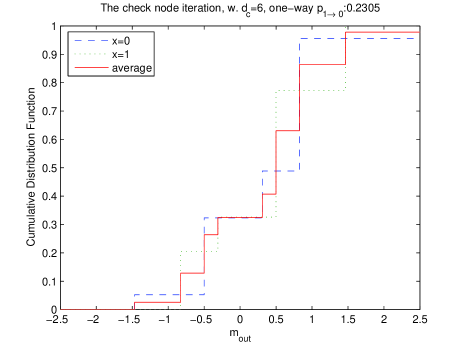
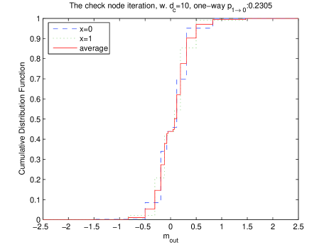
Figure 9: Illustration of the weak convergence of $Q^{(l-1)}_{a.p.}(0)$ and $Q^{(l-1)}_{a.p.}(1)$. One can see that the convergence of $Q^{(l-1)}_{a.p.}(0)$ and $Q^{(l-1)}_{a.p.}(1)$ is faster than the convergence of $\frac{Q^{(l-1)}_{a.p.}(0)+Q^{(l-1)}_{a.p.}(1)}{2}$ and $\delta_{0}$.

VII-B Revisiting the Belief Propagation Decoder

Two known facts about the BP algorithm and the density evolution method are as follows. First, the BP algorithm is optimal for any cycle-free network, since it exploits the independence of the incoming LLR message. Second, by the cycle-free convergence theorem, the traditional density evolution is able to predict the behavior of the BP algorithm (designed for the tree structure) for $l_{0}$ iterations, even when we are focusing on a Tanner graph of a finite-length LDPC code, which inevitably has many cycles. The performance of BP, predicted by density evolution, is outstanding so that we “implicitly assume” that the BP (designed for the tree structure) is optimal for the first $l_{0}$ iterations in terms of minimizing the codeword-averaged bit error rate (BER). Theoretically, to be able to minimize the codeword-averaged BER, the optimal decision rule inevitably must exploit the global knowledge about all possible codewords, which is, however, not available to the BP decoder. A question of interest is whether BP is indeed optimal for the first $l_{0}$ iterations? Namely, with only local knowledge about possible codewords, whether BP has the same performance as the optimal detector with the global information about the entire codebook and unlimited computational power when we are only interested in the first $l_{0}$ iterations? The answer is a straightforward corollary to Theorem 2, the convergence to perfect projection, which provides the missing link regarding the optimality of BP when only local observations (on the ${\mathcal{N}}^{2l})$ are available.

Theorem 8 (Local Optimality of the BP Decoder)

Fix $i,l_{0}\in{\mathbb{N}}$. For sufficiently large codeword length $n$, almost all instances in the random code ensemble have the property that the BP decoder for $x_{i}$ after $l_{0}$ iterations, $\hat{X}_{BP}({\mathbf{Y}}^{l_{0}})$, coincides with the optimal MAP bit detector $\hat{X}_{MAP,l_{0}}({\mathbf{Y}}^{l_{0}})$, where $l_{0}$ is a fixed integer. The MAP bit detector $\hat{X}_{MAP,l_{0}}(\cdot)$ uses the same number of observations as in $\hat{X}_{BP}(\cdot)$ but is able to exploit the global knowledge about the entire codebook.

Proof: When the support tree ${\mathcal{N}}^{2l_{0}}_{(i,j)}$ is perfectly projected, the local information about the tree-satisfying strings is equivalent to the global information about the entire codebook. Therefore, the extra information about the entire codebook does not benefit the decision maker, and $\hat{X}_{BP}(\cdot)=\hat{X}_{MAP,l_{0}}(\cdot)$. Theorem 2 shows that ${\mathcal{N}}^{2l_{0}}_{(i,j)}$ converges to perfect projection in probability, which in turn implies that for sufficiently large $n$, BP decoder is locally optimal for almost all instances of the code ensemble.  ∎

Note: Even when limiting ourselves to symmetric memoryless channels, this local optimality of BP can only be proved by the convergence to perfect projection. Theorem 8 can thus be viewed as a completion of the classical density evolution for symmetric memoryless channels.

VIII Conclusions

In this paper, we have developed a codeword-averaged density evolution, which allows analysis of general non-symmetric memoryless channels. An essential perfect projection convergence theorem has been proved by a constraint propagation argument and by analyzing the behavior of random matrices. With this perfect projection convergence theorem, the theoretical foundation of the codeword-averaged density evolution is well established. Most of the properties of symmetric density evolution have been generalized and proved for the codeword-averaged density evolution on non-symmetric channels, including monotonicity, distribution symmetry, and stability. Besides a necessary stability condition, a sufficient stability condition has been stated with convergence rate arguments and a simple proof.

The typicality of the linear LDPC code ensemble has been proved by the weak convergence (w.r.t. $d_{c}$) of the evolved densities in our codeword-averaged density evolution. Namely, when the check node degree is sufficiently large (e.g. $d_{c}\geq 6$), the performance of the linear LDPC code ensemble is very close to (e.g. within $0.05\%$) the performance of the LDPC coset code ensemble. One important corollary to the perfect projection convergence theorem is the optimality of the belief propagation algorithms when the global information about the entire codebook is accessible. This can be viewed as a completion of the theory of classical density evolution for symmetric memoryless channels.

Extensive simulations have been presented, the degree distribution has been optimized for z-channels, and possible applications of our results have been discussed as well. From both practical and theoretical points of view, our codeword-averaged density evolution offers a straightforward and successful generalization of the traditional symmetric density evolution for general non-symmetric memoryless channels.

Appendix A Proof of Theorem 2

We first introduce the following corollary:

Corollary 6 (Cycle-free Convergence)

For a sequence $l_{n}=\frac{4}{9}\frac{\ln n}{\ln(d_{v}-1)+\ln(d_{c}-1)}$, we have for any $i_{0},j_{0}$,

$${{\mathsf{P}}}\left(\mbox{${\mathcal{N}}^{2l_{n}}_{(i_{0},j_{0})}$ is cycle-free}\right)=1-{\mathcal{O}}\left(n^{-1/9}\right).$$

Proof of Theorem 2: In this proof, the subscript $(i_{0},j_{0})$ will be omitted for notational simplicity.

We notice that if for any $l_{n}\geq l$, ${\mathcal{N}}^{2l_{n}}$ is perfectly projected, then so is ${\mathcal{N}}^{2l}$. Choose $l_{n}=\frac{4}{9}\frac{\ln n}{\ln(d_{v}-1)+\ln(d_{c}-1)}$. By Corollary 6, we have

$${{\mathsf{P}}}(\mbox{${\mathcal{N}}^{2l}$ is perfectly projected})$$

$$\geq{{\mathsf{P}}}(\mbox{${\mathcal{N}}^{2l_{n}}$ is perfectly projected})$$

$$\geq{{\mathsf{P}}}\left(\left.\mbox{${\mathcal{N}}^{2l_{n}}$ is perfectly projected}\right|\mbox{${\mathcal{N}}^{2(l_{n}+1)}$ is cycle-free}\right)$$

$$~{}~{}~{}\cdot{{\mathsf{P}}}\left(\mbox{${\mathcal{N}}^{2(l_{n}+1)}$ is cycle-free}\right)$$

$$={{\mathsf{P}}}\left(\left.\mbox{${\mathcal{N}}^{2l_{n}}$ is perfectly projected}\right|\mbox{${\mathcal{N}}^{2(l_{n}+1)}$ is cycle-free}\right)$$

$$~{}~{}~{}\cdot\left(1-{\mathcal{O}}\left(n^{-1/9}\right)\right).$$

We then need only to show that

$${{\mathsf{P}}}(\mbox{${\mathcal{N}}^{2l_{n}}$ is perfectly projected}|\mbox{${\mathcal{N}}^{2(l_{n}+1)}$ is cycle-free})$$ (28)

$$= 1-{\mathcal{O}}\left(n^{-0.1}\right).$$

To prove (28), we take a deeper look at the incidence matrix (the parity check matrix) $\mathbf{A}$, and use the $(3,5)$ regular code as our illustrative example. The proof is nonetheless general for all regular code ensembles. Conditioning on the event that the graph is cycle-free until depth $2\cdot 2$, we can transform $\mathbf{A}$ into the form of (29) by row and column swaps. Using $\otimes$ to denote the Kronecker product (whether it represents convolution or Kronecker product should be clear from the context), (29) can be further expressed as follows.

$${\mathbf{A}}\tiny=\tiny\left[\vbox{\hbox{\kern-1.15198pt\raise 0.0pt\hbox{\kern 116.25pt}\kern 0.0pt\vbox{}\kern-1.15198pt}}\right]\normalsize$$ (29)

$${\mathbf{A}}~{}=\hskip 227.62204pt$$

$$\left(\begin{array}[]{c|c|c}{\mathbf{I}}_{1\times 1}\otimes(1,1,1,1,1)&{\mathbf{0}}&{\mathbf{0}}\\ \hline\cr{\mathbf{I}}_{5\times 5}\otimes{1\choose 1}&{\mathbf{I}}_{10\times 10}\otimes(1,1,1,1)&{\mathbf{0}}\\ \hline\cr{\mathbf{0}}&{\mathbf{I}}_{40\times 40}\otimes{1\choose 1}&{\mathbf{A}}^{\prime}_{80\times(n-45)}\\ \hline\cr{\mathbf{0}}&{\mathbf{0}}&{\mathbf{A}}^{\prime\prime}_{(\frac{3n}{5}-91)\times(n-45)}\\ \end{array}\right),$$ (34)

where ${\mathbf{I}}_{a\times a}$ denotes the $a\times a$ identity matrix, $\left(\begin{array}[]{c}{\mathbf{A}}^{\prime}_{80\times(n-45)}\\ {\mathbf{A}}^{\prime\prime}_{(\frac{3n}{5}-91)\times(n-45)}\end{array}\right)$ is the incidence matrix of the equiprobable, bipartite subgraph, in which all $(n-45)$ variable nodes have degree $d_{v}$, $80$ check nodes have degree $d_{c}-1$, and $(\frac{3n}{5}-91)$ check nodes have degree $d_{c}$. Conditioning on a more general event that the graph is cycle free until depth $2(l_{n}+1)$ rather than $2\cdot 2$, we will have

$${{\mathbf{A}}}\tiny=\hskip 241.84842pt$$

$$\left(\begin{array}[]{c|c|c|c}\lx@intercol\hfil{\mathbf{A}}_{l_{n}}\hfil\lx@intercol\vrule\lx@intercol&{\mathbf{0}}&{\mathbf{0}}\\ \hline\cr{\mathbf{0}}&{\mathbf{I}}_{(5\cdot 8^{l_{n}-1})\times(5\cdot 8^{l_{n}-1})}\otimes{1\choose 1}&{\mathbf{I}}_{(10\cdot 8^{l_{n}-1})\times(10\cdot 8^{l_{n}-1})}(1,1,1)&{\mathbf{0}}\\ \hline\cr\lx@intercol\hfil{\mathbf{0}}\hfil\lx@intercol\vrule\lx@intercol&{\mathbf{I}}_{(5\cdot 8^{l_{n}})\times(5\cdot 8^{l_{n}})}\otimes{1\choose 1}&{\mathbf{A}}^{\prime}\\ \hline\cr\lx@intercol\hfil{\mathbf{0}}\hfil\lx@intercol\vrule\lx@intercol&{\mathbf{0}}&{\mathbf{A}}^{\prime\prime}\end{array}\right),$$ (39)

where ${\mathbf{A}}_{l_{n}}$ corresponds to the incidence matrix of the cycle-free graph of depth $2l_{n}$. ${{\mathbf{A}}^{\prime}\choose{\mathbf{A}}^{\prime\prime}}$ is the incidence matrix with rows (check nodes) in ${\mathbf{A}^{\prime}}$ and ${\mathbf{A}}^{\prime\prime}$ having degree $(d_{c}-1)$ and $d_{c}$. For convenience, we denote the blocks in $\mathbf{A}$ as

$${\mathbf{A}}=\left(\begin{array}[]{c|c|c|c}\lx@intercol\hfil{\mathbf{A}}_{l_{n}}\hfil\lx@intercol\vrule\lx@intercol&{\mathbf{0}}&{\mathbf{0}}\\ \hline\cr{\mathbf{0}}&{\mathbf{T}}_{l_{n}}&{\mathbf{U}}_{l_{n}+1}&{\mathbf{0}}\\ \hline\cr\lx@intercol\hfil{\mathbf{0}}\hfil\lx@intercol\vrule\lx@intercol&{\mathbf{T}}_{l_{n}+1}&{\mathbf{A}}^{\prime}\\ \hline\cr\lx@intercol\hfil{\mathbf{0}}\hfil\lx@intercol\vrule\lx@intercol&{\mathbf{0}}&{\mathbf{A}}^{\prime\prime}\end{array}\right).$$ (44)

Then ${\mathcal{N}}^{2l_{n}}$ is not perfectly projected if and only if there exists a non-zero row vector $({\mathbf{r}}|{\mathbf{0}}|{\mathbf{0}})$ such that

$$({\mathbf{r}}|{\mathbf{0}}|{\mathbf{0}})\in\mbox{RowSpace}\left(\begin{array}[]{c|c|c|c}{\mathbf{0}}&{\mathbf{T}}_{l_{n}}&{\mathbf{U}}_{l_{n}+1}&{\mathbf{0}}\\ \hline\cr\lx@intercol\hfil{\mathbf{0}}\hfil\lx@intercol\vrule\lx@intercol&{\mathbf{T}}_{l_{n}+1}&{\mathbf{A}}^{\prime}\\ \hline\cr\lx@intercol\hfil{\mathbf{0}}\hfil\lx@intercol\vrule\lx@intercol&{\mathbf{0}}&{\mathbf{A}}^{\prime\prime}\par\par\end{array}\right),$$ (48)

and

$${\mathbf{r}}\mbox{ is not in the row space of ${\mathbf{A}}_{l_{n}}$},$$

$$\mbox{or equivalently $(\mathbf{r}|{\mathbf{0}}|{\mathbf{0}})$ is not in RowSpace(${\mathbf{A}}_{l_{n}}|{\mathbf{0}}|{\mathbf{0}}$)}.$$

(49)

Eqs. (49) and (48) say that there exists a constraint $\mathbf{r}$ on the variable nodes of ${\mathcal{N}}^{2l_{n}}$, which is not from the linear combination of those check node equations within ${\mathcal{N}}^{2l_{n}}$, but rather is imposed by the parity check equations outside ${\mathcal{N}}^{2l_{n}}$. It can be easily proved that if the matrix ${{\mathbf{A}}^{\prime}\choose{\mathbf{A}}^{\prime\prime}}$ is of full row rank, then no such $\mathbf{r}$ exists and ${\mathcal{N}}^{2l_{n}}$ is perfectly projected. Instead of proving ${{\mathbf{A}}^{\prime}\choose{\mathbf{A}}^{\prime\prime}}$ is of full rank, we take a different approach, which takes care of the constraint propagation.

From (48), we know that, for $(\mathbf{r}|{\mathbf{0}}|{\mathbf{0}})$ to exist, there must exist a non-zero row vector $({\mathbf{0}}|{\mathbf{s}}|{\mathbf{0}})$ such that

$$({\mathbf{0}}|{\mathbf{s}}|{\mathbf{0}})\in\mbox{RowSpace}\left(\begin{array}[]{c|c|c|c}\lx@intercol\hfil{\mathbf{0}}\hfil\lx@intercol\vrule\lx@intercol&{\mathbf{T}}_{l_{n}+1}&{\mathbf{A}}^{\prime}\\ \hline\cr\lx@intercol\hfil{\mathbf{0}}\hfil\lx@intercol\vrule\lx@intercol&{\mathbf{0}}&{\mathbf{A}}^{\prime\prime}\par\par\end{array}\right),$$ (52)

and

$${\mathbf{s}} \in \mbox{RowSpace}({\mathbf{U}}_{l_{n}+1})$$

$$= \mbox{RowSpace}\left(I_{(10\cdot 8^{l_{n}-1})\times(10\cdot 8^{l_{n}-1})}\otimes(1,1,1,1)\right).$$

From (LABEL:eq:aligned-bits), the 1’s in $\mathbf{s}$ must be aligned such that four neighboring bits should have the same value; for example, ${\mathbf{s}}=(111100001111000000001111\cdots 00001111)$.

Any non-zero $\mathbf{s}$ satisfying (52) is generated by ${\mathbf{T}}_{l_{n}+1}$. By applying the row symmetry in ${\mathbf{A}}^{\prime}$, we see that the 1’s in any ${\mathbf{s}}$ are uniformly distributed among all these $5\cdot 8^{l_{n}}$ bits. Therefore, conditioning on the event that there exists a not-all-one $\mathbf{s}$ satisfying Eq. (52), the probability that $\mathbf{s}$ satisfies Eq. (LABEL:eq:aligned-bits) is

$${\mathsf{P}}\left(\mbox{$\mathbf{s}$ satisfies Eq.~{}(\ref{eq:aligned-bits})}|\mbox{$\exists\mathbf{s}$ satisfies Eq.~{}(\ref{eq:outside-constraints}) and is not $\mathbf{1}$}\right)$$ (54)

$$= {\mathsf{P}}\left(\mbox{the 1's in ${\mathbf{s}}$ are aligned}|\right.$$

$$\hskip 56.9055pt\left.\mbox{$\exists\mathbf{s}$ satisfies Eq.~{}(\ref{eq:outside-constraints}) and is not $\mathbf{1}$}\right)$$

$$= \sum_{a=1}^{10\cdot 8^{l_{n}-1}-1}\frac{{10\cdot 8^{l_{n}-1}\choose a}}{{5\cdot 8^{l_{n}}\choose 4a}}\cdot{\mathsf{P}}(\mbox{there are $4a$ ones in ${\mathbf{s}}$})$$

$$\leq \frac{{10\cdot 8^{l_{n}-1}\choose 1}}{{5\cdot 8^{l_{n}}\choose 4}}{{\mathcal{O}}}\left(\left(\frac{1}{((d_{v}-1)(d_{c}-1))^{l_{n}}}\right)^{d_{c}-2}\right)$$

$$= {{\mathcal{O}}}\left(n^{-\frac{4}{9}(d_{c}-2)}\right).$$

The last inequality follows from the assumption that ${\mathbf{s}}$ is neither all-zero nor all-one. The reason why we can exclude the case that $\mathbf{s}$ is all-one is that, if $d_{v}$ is odd, then there is an even number of 1’s in each column of ${\mathbf{T}}_{l_{n}}$. Since there is only one 1 in each column of ${\mathbf{U}}_{l_{n}+1}$, by (48), an all-one $\mathbf{s}$ can only generate an all-zero ${\mathbf{r}}$, which puts no constraints on ${\mathcal{N}}^{2l_{n}}_{(i_{0},j_{0})}$. If $d_{v}$ is even, by the same reasoning, an all-one $\mathbf{s}$ will generate ${\mathbf{r}}$ of the form $(00\cdots 0\overbrace{11\cdots 1}^{5\cdot 8^{l_{n}-1}})$. Nevertheless, when $d_{v}$ is even, this specific type of $\mathbf{r}$ is in the row space of ${\mathbf{A}}_{l_{n}}$, which does not fulfill the requirement in (49). From the above reasoning, we can exclude the all-one $\mathbf{s}$.

Let $m_{r}$ denote the number of rows of ${{\mathbf{A}}^{\prime}\choose{\mathbf{A}}^{\prime\prime}}$ minus $\mathop{\rm Rank}\limits({{\mathbf{A}}^{\prime}\choose{\mathbf{A}}^{\prime\prime}})$. The number of vectors $\mathbf{s}$ satisfying (52) is upper bounded by $2^{m_{r}}$. By (54), Proposition 4 (which will be formally stated and proved later), and the union bound, we have

$${{\mathsf{P}}}(\mbox{${\mathcal{N}}^{2l_{n}}_{(i_{0},j_{0})}$ is not perfectly projected}|\mbox{${\mathcal{N}}^{2(l_{n}+1)}_{(i_{0},j_{0})}$ is cycle-free})$$ (55)

$$= {{\mathsf{P}}}(\mbox{$\exists{\mathbf{r}}$ satisfying (\ref{eq:full-rank-equivalent-1}) and (\ref{eq:full-rank-equivalent-2})})$$

$$= {{\mathsf{P}}}(\mbox{$\exists{\mathbf{s}}$, which satisfies (\ref{eq:outside-constraints}) and (\ref{eq:aligned-bits}), but is not all-one})$$

$$\leq n^{1.1}\cdot{\mathsf{P}}\left(\mbox{$\mathbf{s}$ satisfies Eq.~{}(\ref{eq:aligned-bits})}|\right.$$

$$\hskip 56.9055pt\left.\mbox{$\exists\mathbf{s}$ satisfies Eq.~{}(\ref{eq:outside-constraints}) and is not $\mathbf{1}$}\right)$$

$$\cdot{\mathsf{P}}\left(\mbox{\# of $\mathbf{s}$ is smaller than $n^{1.1}$}\right)$$

$$+{\mathsf{P}}\left(\mbox{\# of $\mathbf{s}$ is larger than $n^{1.1}$}\right)$$

$$= n^{1.1}{\mathcal{O}}(n^{-\frac{4}{9}(d_{c}-2)})+{{\mathsf{P}}}(2^{m_{r}}>n^{1.1})$$

$$= {\mathcal{O}}(n^{-0.1}),~{}~{}\forall d_{c}\geq 5.$$

To prove the case $d_{c}<5$, we focus on the probability that the constraints propagate two levels rather than just one level, i.e. instead of (28), we focus on proving the following statement:

$${{\mathsf{P}}}(\mbox{${\mathcal{N}}^{2l_{n}}_{(i_{0},j_{0})}$ is perfectly projected}|\mbox{${\mathcal{N}}^{2(l_{n}+2)}_{(i_{0},j_{0})}$ is cycle-free})$$

$$= 1-{\mathcal{O}}\left(n^{-0.1}\right).$$

Most of the analysis remains the same. The conditional probability in (54) will be replaced by

$${{\mathsf{P}}}(\mbox{$({\mathbf{0}}|{\mathbf{s}}|{\mathbf{0}})$ is able to propagate two levels}|\mbox{$\exists\mathbf{s}$ satisfying (\ref{eq:outside-constraints})})$$

$$= {{\mathsf{P}}}(\mbox{$({\mathbf{0}}|{\mathbf{s}}|{\mathbf{0}})$ propagates the 2nd level}|$$

$$~{}~{}~{}~{}~{}\mbox{$({\mathbf{0}}|{\mathbf{s}}|{\mathbf{0}})$ propagates the 1st level},\mbox{$\exists\mathbf{s}$ satisfying (\ref{eq:outside-constraints})})$$

$$\cdot{{\mathsf{P}}}(\mbox{$({\mathbf{0}}|{\mathbf{s}}|{\mathbf{0}})$ propagates the 1st level}|\mbox{$\exists\mathbf{s}$ satisfying (\ref{eq:outside-constraints})})$$

$$= \sum_{a,b}\frac{{10\cdot 8^{l_{n}-1}\choose a}}{{5\cdot 8^{l_{n}}\choose 4a}}\frac{{10\cdot 8^{l_{n}}\choose b}}{{5\cdot 8^{l_{n}+1}\choose 4b}}$$

$$~{}\cdot{\mathsf{P}}(\mbox{$4a$ and $4b$ 1's to propagate the 2nd and 1st levels})$$

$$\stackrel{{\scriptstyle(a)}}{{\leq}} \frac{{10\cdot 8^{l_{n}-1}\choose 1}}{{5\cdot 8^{l_{n}}\choose 4}}\frac{{10\cdot 8^{l_{n}1}\choose 4}}{{5\cdot 8^{l_{n}+1}\choose 4\cdot 4}}$$

$$= {\mathcal{O}}\left(n^{-\frac{4}{9}(d_{c}^{2}-2d_{c})}\right),$$

where the inequality marked (a) follows from an analysis of the minimum number of bits required for the constraint propagation similar to that for the single level case. By this stronger inequality and a bounding inequality similar to that in (55), we thus complete the proof of the case $d_{c}\geq 3$ for all regular codes of practical interest.

∎

Note: This constraint propagation argument shows that the convergence to a perfectly projected tree is very strong. Even for codes with redundant check node equations (not of full row rank), it is probabilistically hard for the external constraints to propagate inside and impose on the variable nodes within ${\mathcal{N}}^{2l}$. This property is helpful when we consider belief propagation decoding on the alternative graph representation as in [40].

We close this section by stating the proposition regarding $m_{r}$, the number of linearly dependent rows in ${{\mathbf{A}}^{\prime}\choose{\mathbf{A}}^{\prime\prime}}$. The proof is left to Appendix B.

Proposition 4

Consider the semi-regular code ensemble ${\mathcal{C}}^{n}_{m^{\prime},m^{\prime\prime}}(d_{v},d_{c})$ generated by equiprobable edge permutation on a bipartite graph with $n$ variable nodes of degree $d_{v}$, and $m^{\prime}$ and $m^{\prime\prime}$ check nodes with respective degrees $(d_{c}-1)$ and $d_{c}$. The corresponding parity check matrix is ${\mathbf{A}}={{\mathbf{A}}^{\prime}\choose{\mathbf{A}}^{\prime\prime}}$. With $m_{r}$ denoting the number of linearly dependent rows in ${\mathbf{A}}$, i.e. $m_{r}:=m^{\prime}+m^{\prime\prime}-\mathop{\rm Rank}\limits({\mathbf{A}})$, we have

$${{\mathsf{E}}}\{2^{m_{r}}\}={\mathcal{O}}(n),$$

which automatically implies ${{\mathsf{P}}}\left(2^{m_{r}}>n^{1+\alpha}\right)={{\mathsf{P}}}\left(m_{r}>\frac{(1+\alpha)\ln n}{\ln 2}\right)={\mathcal{O}}(n^{-\alpha})$, for any $\alpha>0$.

Corollary 7

Let $R$ denote the rate of a regular LDPC code ensemble ${\mathcal{C}}^{n}(d_{v},d_{c})$, i.e., $R=\frac{n-\mathop{\rm Rank}\limits({\mathbf{A}})}{n}$, where $\mathbf{A}$ is the corresponding parity check matrix. Then $R$ converges to $(n-m)/n$ in $L^{1}$, i.e.

$$\lim_{n\rightarrow\infty}{\mathsf{E}}\left\{\left|R-\frac{n-m}{m}\right|\right\}=0.$$

Proof:

It is obvious that $R\geq\frac{n-m}{n}$. To show that $\limsup_{n\rightarrow\infty}{\mathsf{E}}\{R-\frac{n-m}{n}\}=0$, we let $m_{1}=0$ and rewrite $R=\frac{n-\mathop{\rm Rank}\limits({\mathbf{A}})}{n}=\frac{n-m}{n}+\frac{m_{r}}{n}$. By Proposition 4 and the fact that $\frac{m_{r}}{n}\leq 1$, we have $\lim_{n\rightarrow\infty}{\mathsf{E}}\{\frac{m_{r}}{n}\}=0$. This completes the proof. ∎

A stronger version of the convergence of $R$ with respect to the block length $n$ can be found in [39].

Appendix B Proof of Proposition 4

We finish the proof of Proposition 4 by first stating the following lemma.

Lemma 2

For all $0<k\in{\mathbb{N}},0<i<n\in{\mathbb{N}}$, we have

$$\frac{{n\choose i}}{{kn\choose ki}}\leq\sqrt{k}e^{\frac{1}{6}}2^{-(k-1)nH_{2}(i/n)}.$$

Proof: By Stirling’s double inequality,

$$\sqrt{2\pi}n^{(n+\frac{1}{2})}e^{(-n+\frac{1}{12n+1})}<n!<\sqrt{2\pi}n^{(n+\frac{1}{2})}e^{(-n+\frac{1}{12n})},$$

we can prove

$$e^{-\frac{1}{6}}<\frac{{n\choose\theta n}}{\frac{1}{\sqrt{2\pi}}2^{nH_{2}(i/n)}\sqrt{\frac{n}{i(n-i)}}}<1,$$

which immediately leads to the desired inequality.  ∎

Proof of Proposition 4: By the definition of $m_{r}$, we have $2^{m_{r}}=(\mbox{total \# of codewords})/2^{n-m}$, where $m=m^{\prime}+m^{\prime\prime}$. Then

$${\mathsf{E}}\left\{\frac{2^{m_{r}}}{n}\right\}\leq\frac{2}{n2^{n-m}}+\sum_{i=1}^{n-1}\frac{{\mathsf{E}}\left\{\mbox{\# of codewords of weight $i$}\right\}}{n2^{n-m}}.$$

Using the enumerating function as in [41, 39] and define $g(x)$ as

$$g(i,x):=\frac{\left(\frac{(1+x)^{d_{c}-1}+(1-x)^{d_{c}-1}}{2}\right)^{m^{\prime}}\left(\frac{(1+x)^{d_{c}}+(1-x)^{d_{c}}}{2}\right)^{m^{\prime\prime}}}{x^{id_{v}}},$$

the above quantity can be further upper bounded as follows.

$${\mathsf{E}}\left\{\frac{2^{m_{r}}}{n}\right\}$$

$$\leq \frac{2}{n2^{n-m}}+\sum_{i=1}^{n-1}\frac{\frac{{n\choose i}}{{nd_{v}\choose id_{v}}}\inf_{x>0}g(i,x)}{n2^{n-m}}$$

$$\leq \frac{2}{n2^{n-m}}+\sqrt{d_{v}}e^{1/6}\sum_{i=1}^{n-1}\frac{1}{n}2^{-(d_{v}-1)nH_{2}(i/n)}\frac{\inf_{x>0}g(i,x)}{2^{n-m}}$$

$$\leq \frac{2}{n2^{n-m}}+\sqrt{d_{v}}e^{1/6}\sum_{i=1}^{n-1}\frac{1}{n}2^{-d_{v}nH_{2}(i/n)}\frac{\inf_{x>0}g(i,x)}{2^{-m}},$$

where the second inequality follows from Lemma 2 and the third inequality follows from the fact that the binary entropy function $H_{2}(\cdot)$ is upper bounded by 1.

By defining

$$f_{n}(i,x):=2^{m-d_{v}nH_{2}(i/n)}g(i,x),$$

the summation in (LABEL:eq:sum-of-f) is upper bounded by

$$\max_{i\in[0,n]}\inf_{x>0}f_{n}(i,x)\leq\inf_{x>0}\max_{i\in[0,n]}f_{n}(i,x)\leq\max_{i\in[0,n]}f_{n}(i,1).$$

By simple calculus, $\max_{i\in[0,n]}f_{n}(i,1)$ is attained when $i=n/2$. Since $f_{n}(n/2,1)=1$, the summation in (LABEL:eq:sum-of-f) is bounded by 1 for all $n$, and therefore

$$\limsup_{n\rightarrow\infty}{\mathsf{E}}\left\{\frac{2^{m_{r}}}{n}\right\}\leq\sqrt{d_{v}}e^{1/6}.$$

The proof is complete.

∎

Appendix C Proof of Corollary 5

We prove one direction that

$$p^{*}_{1\rightarrow 0,linear} := \sup\left\{p_{1\rightarrow 0}>0:\lim_{l\rightarrow\infty}p_{e,linear}^{(l)}=0\right\}$$

$$> \sup\left\{p_{1\rightarrow 0}>0:\lim_{l\rightarrow\infty}p_{e,coset}^{(l)}=0\right\}-\epsilon$$

$$:= p^{*}_{1\rightarrow 0,coset}-\epsilon.$$

The other direction that $p^{*}_{1\rightarrow 0,coset}>p^{*}_{1\rightarrow 0,linear}-\epsilon$ can be easily obtained by symmetry.

By definition, for any $\epsilon>0$, we can find a sufficiently large $l_{0}<\infty$ such that for a z-channel with one-way crossover probability $p_{1\rightarrow 0}:=p^{*}_{1\rightarrow 0,coset}-\epsilon$, $P^{(l_{0})}_{coset}$ is in the interior of the stability region. We note that the stability region depends only on the Bhattacharyya noise parameter of $P^{(l_{0})}_{coset}$, which is a continuous function with respect to convergence in distribution. Therefore, by Theorem 7, there exists a $\Delta\in{\mathbb{N}}$ such that $\left\langle P^{(l_{0})}\right\rangle$ is also in the stability region. By the definition of the stability region, we have $\lim_{l\rightarrow\infty}p_{e,linear}^{(l)}=0$, which implies $p^{*}_{1\rightarrow 0,linear}\geq p_{1\rightarrow 0}$. The proof is thus complete.

Appendix D The Convergence Rates of (26) and (27)

For (26), we will consider the cases that $k=0$ and $k=1$ separately. By the BASC decomposition argument, namely, all non-symmetric channels can be decomposed as the probabilistic combination of many BASCs, we can limit our attention to simple BASCs rather than general memoryless non-symmetric channels. Suppose $P^{(l-1)}_{a.p.}(0)$ and $P^{(l-1)}_{a.p.}(1)$ correspond to a BASC with crossover probabilities $\epsilon_{0}$ and $\epsilon_{1}$. Without loss of generality, we may assume $\epsilon_{0}+\epsilon_{1}<1$ because of the previous assumption that $\forall x\in\mathop{\sf GF}\limits(2),P^{(l-1)}_{a.p.}(x)(m=0)=0$. We then have

$$\Phi_{P^{\prime}_{0}}(k,\frac{r}{\Delta}) = (1-\epsilon_{0})e^{i\frac{r}{\Delta}\ln\frac{1-\epsilon_{0}+\epsilon_{1}}{1-\epsilon_{0}-\epsilon_{1}}}$$

$$+(-1)^{k}\epsilon_{0}e^{i\frac{r}{\Delta}\ln\frac{1+\epsilon_{0}-\epsilon_{1}}{1-\epsilon_{0}-\epsilon_{1}}}$$

$$\mbox{and~{}~{}}\Phi_{P^{\prime}_{1}}(k,\frac{r}{\Delta}) = (1-\epsilon_{1})e^{i\frac{r}{\Delta}\ln\frac{1+\epsilon_{0}-\epsilon_{1}}{1-\epsilon_{0}-\epsilon_{1}}}$$

$$+(-1)^{k}\epsilon_{1}e^{i\frac{r}{\Delta}\ln\frac{1-\epsilon_{0}+\epsilon_{1}}{1-\epsilon_{0}-\epsilon_{1}}}.$$

By Taylor’s expansion, for $k=0$, (26) becomes

$$2\left(\frac{\Phi_{P^{\prime}_{0}}(0,\frac{r}{\Delta})-\Phi_{P^{\prime}_{1}}(0,\frac{r}{\Delta})}{2}\right)^{\Delta}$$

$$= 2\left(i\left(\frac{1-\epsilon_{0}-\epsilon_{1}}{2}\right)\left(\frac{r}{\Delta}\right)\ln\left(\frac{1-\epsilon_{0}+\epsilon_{1}}{1+\epsilon_{0}-\epsilon_{1}}\right)\right.$$

$$\left.\hskip 125.19194pt+{\mathcal{O}}\left(\left(\frac{r}{\Delta}\right)^{2}\right)\right)^{\Delta},$$

which converges to zero with convergence rate ${\mathcal{O}}\left({\mathcal{O}}(\Delta)^{-\Delta}\right)$. For $k=1$, we have

$$2\left(\frac{\Phi_{P^{\prime}_{0}}(1,\frac{r}{\Delta})-\Phi_{P^{\prime}_{1}}(1,\frac{r}{\Delta})}{2}\right)^{\Delta}$$

$$= 2\left(\left(\epsilon_{1}-\epsilon_{0}\right)+\frac{i}{2}\left(\frac{r}{\Delta}\right)\left((1-\epsilon_{0}+\epsilon_{1})\ln\frac{1-\epsilon_{0}+\epsilon_{1}}{1-\epsilon_{0}-\epsilon_{1}}\right.\right.$$

$$\left.\hskip 85.35826pt-(1+\epsilon_{0}-\epsilon_{1})\ln\frac{1+\epsilon_{0}-\epsilon_{1}}{1-\epsilon_{0}-\epsilon_{1}}\right)$$

$$\left.~{}~{}~{}~{}+{\mathcal{O}}\left(\left(\frac{r}{\Delta}\right)^{2}\right)\right)^{\Delta},$$

which converges to zero with convergence rate ${\mathcal{O}}({\mathsf{const}}^{\Delta})$, where ${\mathsf{const}}$ satisfies $|\epsilon_{1}-\epsilon_{0}|<{\mathsf{const}}<1$. Since the convergence rate is determined by the slower of the above two, we have proven that (26) converges to zero with rate ${\mathcal{O}}({\mathsf{const}}^{\Delta})$ for some ${\mathsf{const}}<1$.

Consider (27). Since we assume that the input is not perfect, we have $\max(\epsilon_{0},\epsilon_{1})>0$. For $k=0$, by Taylor’s expansion, we have

$$\left(\frac{\Phi_{P^{\prime}_{0}}(0,\frac{r}{\Delta})+\Phi_{P^{\prime}_{1}}(0,\frac{r}{\Delta})}{2}\right)^{\Delta}$$

$$= \left(1+\frac{i}{2}\left(\frac{r}{\Delta}\right)\left((1-\epsilon_{0}+\epsilon_{1})\ln\frac{1-\epsilon_{0}+\epsilon_{1}}{1-\epsilon_{0}-\epsilon_{1}}\right.\right.$$

$$\left.\hskip 85.35826pt+(1+\epsilon_{0}-\epsilon_{1})\ln\frac{1+\epsilon_{0}-\epsilon_{1}}{1-\epsilon_{0}-\epsilon_{1}}\right)$$

$$\left.~{}~{}~{}~{}+{\mathcal{O}}\left(\left(\frac{r}{\Delta}\right)^{2}\right)\right)^{\Delta},$$

which converges to

$$e^{i\left(\frac{r}{2}\right)\left((1-\epsilon_{0}+\epsilon_{1})\ln\frac{1-\epsilon_{0}+\epsilon_{1}}{1-\epsilon_{0}-\epsilon_{1}}+(1+\epsilon_{0}-\epsilon_{1})\ln\frac{1+\epsilon_{0}-\epsilon_{1}}{1-\epsilon_{0}-\epsilon_{1}}\right)}$$

with rate ${\mathcal{O}}\left(\Delta^{-1}\right)$. For $k=1$, we have

$$\left(\frac{\Phi_{P^{\prime}_{0}}(1,\frac{r}{\Delta})+\Phi_{P^{\prime}_{1}}(1,\frac{r}{\Delta})}{2}\right)^{\Delta}$$

$$= \left(\left(1-\epsilon_{0}-\epsilon_{1}\right)\left(\frac{e^{i\frac{r}{\Delta}\ln\frac{1-\epsilon_{0}+\epsilon_{1}}{1-\epsilon_{0}-\epsilon_{1}}}+e^{i\frac{r}{\Delta}\ln\frac{1+\epsilon_{0}-\epsilon_{1}}{1-\epsilon_{0}-\epsilon_{1}}}}{2}\right)\right)^{\Delta},$$

which converges to zero with rate ${\mathcal{O}}\left((1-\epsilon_{0}-\epsilon_{1})^{\Delta}\right)$. Since the overall convergence rate is the slower of the above two, we have proven that the convergence rate is ${\mathcal{O}}\left(\Delta^{-1}\right)$.

Chih-Chun Wang received the B.E. degree in E.E. from National Taiwan University, Taipei, Taiwan in 1999, the M.S. degree in E.E., the Ph.D. degree in E.E. from Princeton University in 2002 and 2005, respectively. He is currently working with Prof. Poor and Prof. Kulkarni in a post-doc position at Princeton University. He worked in COMTREND Corporation, Taipei, Taiwan, from 1999-2000, and spent the summer of 2004 with Flarion Technologies. He will join the ECE department of Purdue University as an assistant professor in January 2006. His research interests are in optimal control, information theory and coding theory, especially on the performance analysis of iterative decoding for LDPC codes.

Sanjeev R. Kulkarni (M’91, SM’96, F’04) received the B.S. in Mathematics, B.S. in E.E., M.S. in Mathematics from Clarkson University in 1983, 1984, and 1985, respectively, the M.S. degree in E.E. from Stanford University in 1985, and the Ph.D. in E.E. from M.I.T. in 1991. From 1985 to 1991 he was a Member of the Technical Staff at M.I.T. Lincoln Laboratory working on the modelling and processing of laser radar measurements. In the spring of 1986, he was a part-time faculty at the University of Massachusetts, Boston. Since 1991, he has been with Princeton University where he is currently Professor of Electrical Engineering. He spent January 1996 as a research fellow at the Australian National University, 1998 with Susquehanna International Group, and summer 2001 with Flarion Technologies. Prof. Kulkarni received an ARO Young Investigator Award in 1992, an NSF Young Investigator Award in 1994, and several teaching awards at Princeton University. He has served as an Associate Editor for the IEEE Transactions on Information Theory. Prof. Kulkarni’s research interests include statistical pattern recognition, nonparametric estimation, learning and adaptive systems, information theory, wireless networks, and image/video processing.

H. Vincent Poor (S’72, M’77, SM’82, F’77) received the Ph.D. degree in EECS from Princeton University in 1977. From 1977 until 1990, he was on the faculty of the University of Illinois at Urbana-Champaign. Since 1990 he has been on the faculty at Princeton, where he is the George Van Ness Lothrop Professor in Engineering. Dr. Poor’s research interests are in the areas of statistical signal processing and its applications in wireless networks and related fields. Among his publications in these areas is the recent book Wireless Networks: Multiuser Detection in Cross-Layer Design (Springer: New York, NY, 2005). Dr. Poor is a member of the National Academy of Engineering and is a Fellow of the American Academy of Arts and Sciences. He is also a Fellow of the Institute of Mathematical Statistics, the Optical Society of America, and other organizations. In 1990, he served as President of the IEEE Information Theory Society, and he is currently serving as the Editor-in-Chief of these Transactions. Recent recognition of his work includes the Joint Paper Award of the IEEE Communications and Information Theory Societies (2001), the NSF Director’s Award for Distinguished Teaching Scholars (2002), a Guggenheim Fellowship (2002-03), and the IEEE Education Medal (2005).

References

- [1] C. Berrou and A. Glavieux, “Near optimum error correcting coding and decoding: Turbo-codes,” IEEE Trans. Inform. Theory, vol. 44, no. 10, pp. 1261–1271, Oct. 1996.
- [2] R. G. Gallager, Low-Density Parity-Check Codes, ser. Research Monograph Series. Cambridge, MA: MIT Press, 1963, no. 21.
- [3] D. J. C. MacKay, “Good error-correcting codes based on very sparse matrices,” IEEE Trans. Inform. Theory, vol. 45, no. 2, pp. 399–431, Mar. 1999.
- [4] M. Sipser and D. A. Spielman, “Expander codes,” IEEE Trans. Inform. Theory, vol. 42, no. 6, pp. 1710–1722, Nov. 1996.
- [5] J. Pearl, Probabilistic Reasoning in Intelligent Systems: Network of Plausible Inference. San Mateo, CA: Morgan Kaufmann, 1988.
- [6] R. J. McEliece, D. J. C. Mackay, and J. F. Cheng, “Turbo decoding as an instance of Pearl’s “Belief Propagation” algorithm,” IEEE J. Select. Areas Commun., vol. 16, no. 2, pp. 140–152, Feb. 1998.
- [7] S. Y. Chung, G. D. Forney, Jr., T. J. Richardson, and R. L. Urbanke, “On the design of low-density parity-check codes within 0.0045 dB of the Shannon limit,” IEEE Commun. Letters, vol. 5, no. 2, pp. 58–60, Feb. 2001.
- [8] T. J. Richardson and R. L. Urbanke, “Efficient encoding of low-density parity-check codes,” IEEE Trans. Inform. Theory, vol. 47, no. 2, pp. 638–656, Feb. 2001.
- [9] D. A. Spielman, “Linear-time encodable and decodable error-correcting codes,” IEEE Trans. Inform. Theory, vol. 42, no. 6, pp. 1723–1731, Nov. 1996.
- [10] J. W. Byers, M. Luby, and M. Mitzenmacher, “A digital fountain approach to asynchronous reliable multicast,” IEEE J. Select. Areas Commun., vol. 20, no. 8, pp. 1528–1540, Oct. 2002.
- [11] M. G. Luby, M. Mitzenmacher, M. A. Shokrollahi, and D. A. Spielman, “Analysis of low-density codes and improved designs using irregular graphs,” in Proc. 30th Annu. ACM Symp. Theory of Computing, 1998, pp. 249–258.
- [12] ——, “Efficient erasure correcting codes,” IEEE Trans. Inform. Theory, vol. 47, pp. 569–584, Feb. 2001.
- [13] T. J. Richardson and R. L. Urbanke, “The capacity of low-density parity-check codes,” IEEE Trans. Inform. Theory, vol. 47, no. 2, pp. 599–618, Feb. 2001.
- [14] J. Hou, P. H. Siegel, and L. B. Milstein, “Performance analysis and code optimization of low density parity-check codes on Rayleigh fading channels,” IEEE J. Select. Areas Commun., vol. 19, no. 5, pp. 924–934, May 2001.
- [15] J. Garcia-Frias, “Decoding of low-density parity check codes over finite-state binary Markov channels,” in Proc. IEEE Int’l. Symp. Inform. Theory. Washington, DC, 2001, p. 72.
- [16] A. Kavčić, X. Ma, and M. Mitzenmacher, “Binary intersymbol interference channels: Gallager codes, density evolution and code performance bound,” IEEE Trans. Inform. Theory, vol. 49, no. 7, pp. 1636–1652, July 2003.
- [17] B. M. Kurkoski, P. H. Siegel, and J. K. Wolf, “Joint message-passing decoding of LDPC codes and partial-response channels,” IEEE Trans. Inform. Theory, vol. 48, no. 6, pp. 1410–1422, June 2002.
- [18] J. Li, K. R. Narayanan, E. Kurtas, and C. N. Georghiades, “On the performance of high-rate TPC/SPC codes and LDPC codes over partial response channels,” IEEE Trans. Commun., vol. 50, no. 5, pp. 723–734, May 2002.
- [19] A. Thangaraj and S. W. McLaughlin, “Thresholds and scheduling for LDPC-coded partial response channels,” IEEE Trans. Magn., vol. 38, no. 5, pp. 2307–2309, Sep. 2002.
- [20] G. Caire, D. Burshtein, and S. Shamai, “LDPC coding for interference mitigation at the transmitter,” in Proc. 40th Annual Allerton Conf. on Comm., Contr., and Computing. Monticello, IL, USA, Oct. 2002.
- [21] J. Hou, P. H. Siegel, L. B. Milstein, and H. D. Pfister, “Capacity-approaching bandwidth-efficient coded modulation schemes based on low-density parity-check codes,” IEEE Trans. Inform. Theory, vol. 49, no. 9, pp. 2141–2155, Sept. 2003.
- [22] C. Di, D. Proietti, E. Telatar, T. J. Richardson, and R. L. Urbanke, “Finite-length analysis of low-density parity-check codes on the binary erasure channel,” IEEE Trans. Inform. Theory, vol. 48, no. 6, pp. 1570–1579, June 2002.
- [23] T. J. Richardson, M. A. Shokrollahi, and R. L. Urbanke, “Design of capacity-approaching irregular low-density parity-check codes,” IEEE Trans. Inform. Theory, vol. 47, no. 2, pp. 619–637, Feb. 2001.
- [24] S. Litsyn and V. Shevelev, “On ensembles of low-density parity-check codes: Asymptotic distance distributions,” IEEE Trans. Inform. Theory, vol. 48, no. 4, pp. 887–908, Apr. 2002.
- [25] H. Jin and R. McEliece, “Coding theorems for turbo code ensembles,” IEEE Trans. Inform. Theory, vol. 48, no. 6, pp. 1451–1461, June 2002.
- [26] F. Lehmann, “Distance properties of irregular LDPC codes,” in Proc. IEEE Int’l. Symp. Inform. Theory. Yokohama, Japan, 2003, p. 85.
- [27] S. Shamai and I. Sason, “Variations on the Gallager bounds, connections, and applications,” IEEE Trans. Inform. Theory, vol. 48, no. 12, pp. 3029–3051, Dec. 2002.
- [28] A. Bennatan and D. Burshtein, “Iterative decoding of LDPC codes over arbitrary discrete-memoryless channels,” in Proc. 41st Annual Allerton Conf. on Comm., Contr., and Computing. Monticello, IL, USA, 2003, pp. 1416–1425.
- [29] A. Bennatan and D. Burstein, “On the application of LDPC codes to arbitrary discrete-memoryless channels,” IEEE Trans. Inform. Theory, vol. 50, no. 3, pp. 417–438, March 2004.
- [30] C. C. Wang, S. R. Kulkarni, and H. V. Poor, “On finite-dimensional bounds for LDPC-like codes with iterative decoding,” in Proc. Int’l Symp. Inform. Theory & its Applications. Parma, Italy, Oct. 2004, submitted to IEEE Trans. Inform. Theory.
- [31] A. Khandekar, “Graph-based codes and iterative decoding,” Ph.D. dissertation, California Institute of Technology, 2002.
- [32] A. Orlitsky, K. Viswanathan, and J. Zhang, “Stopping set distribution of LDPC code ensembles,” in Proc. IEEE Int’l. Symp. Inform. Theory. Yokohama, Japan, 2003, p. 123.
- [33] E. E. Majani and H. Rumsey Jr., “Two results on binary-input discrete memoryless channels,” in Proc. IEEE Int’l. Symp. Inform. Theory. Budapest, Hungary, June 1991, p. 104.
- [34] N. Shulman and M. Feder, “The uniform distribution as a universal prior,” IEEE Trans. Inform. Theory, vol. 50, no. 6, pp. 1356–1362, June 2004.
- [35] R. J. McEliece, “Are turbo-like codes effective on nonstandard channels?” IEEE Inform. Theory Society Newsletter, vol. 51, no. 4, Dec. 2001.
- [36] M. Yang and W. E. Ryan, “Lowering the error-rate floors of moderate-length high-rate irregular LDPC codes,” in Proc. IEEE Int’l. Symp. Inform. Theory. Yokohama, Japan, 2003, p. 237.
- [37] E. Ratzer and D. MacKay, “Sparse low-density parity-check codes for channels with cross-talk,” in Proc. IEEE Inform. Theory Workshop. Paris, France, March 31 – April 4 2003.
- [38] H. Jin and T. J. Richardson, “Fast density evolution,” in Proc. 38th Conf. Inform. Sciences and Systems. Princeton, NJ, USA, 2004.
- [39] G. Miller and G. Cohen, “The rate of regular LDPC codes,” IEEE Trans. Inform. Theory, vol. 49, no. 11, pp. 2989–2992, Nov. 2003.
- [40] V. Kumar, O. Milenkovic, and K. Prakash, “On graphical representations of algebraic codes suitable for iterative decoding,” in Proc. 39th Conf. Inform. Sciences & Systems. Baltimore, MD, USA, March 2005.
- [41] D. Burshtein and G. Miller, “Asymptotic enumeration methods for analyzing LDPC codes,” IEEE Trans. Inform. Theory, vol. 50, no. 6, pp. 1115–1131, June 2004.