Optimal Space-Time Codes for the MIMO Amplify-and-Forward Cooperative Channel

Abstract

In this work, we extend the non-orthogonal amplify-and-forward (NAF) cooperative diversity scheme to the MIMO channel. A family of space-time block codes for a half-duplex MIMO NAF fading cooperative channel with $N$ relays is constructed. The code construction is based on the non-vanishing determinant (NVD) criterion and is shown to achieve the optimal diversity-multiplexing tradeoff (DMT) of the channel. We provide a general explicit algebraic construction, followed by some examples. In particular, in the single-relay case, it is proved that the Golden code and the $4\times 4$ Perfect code are optimal for the single-antenna and two-antenna case, respectively. Simulation results reveal that a significant gain (up to $10$ dB) can be obtained with the proposed codes, especially in the single-antenna case.

Notations

In this paper, we use boldface lower case letters $\boldsymbol{v}$ to denote vectors, boldface capital letters $\boldsymbol{M}$ to denote matrices. $\mathcal{C}\mathcal{N}$ represents the complex Gaussian random variable. $\mathbb{E}[\cdot]$ stands for the expectation operation and ${[\cdot]}^{\scriptscriptstyle\mathsf{T}\!},{[\cdot]}^{\scriptscriptstyle{\dagger}\!}$ denote the matrix transposition and conjugated transposition operations. $\left\|{\cdot}\right\|$ is the Euclidean vector norm and $\left\|{\cdot}\right\|_{\text{F}}$ is the Frobenius matrix norm. $\left|\mathcal{S}\right|$ is the cardinality of the set $\mathcal{S}$. $(x)^{+}$ means $\max(0,x)$. $\mathbb{R}$, $\mathbb{C}$, $\mathbb{Q}$ and $\mathbb{Z}$ stand for the real field, complex field, rational field and the integer ring respectively. For any quantity $q$,

$$q\doteq{\mathsf{SNR}}^{\alpha}\quad\textrm{means}\quad\lim_{{\mathsf{SNR}}\to\infty}\frac{\log q}{\log{\mathsf{SNR}}}=\alpha$$

and similarly for $\ \dot{\leq}\,$ and $\ \dot{\geq}\,$.

I Introduction

On a wireless channel, diversity techniques are used to combat channel fadings. Recently, there has been a growing interest in the so called cooperative diversity techniques, where multiple terminals in a network cooperate to form a virtual antenna array in order to exploit spatial diversity in a distributed fashion. In this manner, spatial diversity gain can be obtained even when a local antenna array is not available. Since the work of [1, 2], several cooperative transmission protocols have been proposed [3, 4, 5, 6, 7, 8, 9]. These protocols can be categorized into two principal classes : the amplify-and-forward (AF) scheme and the decode-and-forward (DF) scheme. In practice, the AF scheme is more attractive for its low complexity since the cooperative terminals (relays) simply forward the signal and do not decode it. Actually, for most ad hoc wireless networks, it is not realistic for other terminals to decode the signal from a certain user, because the codebook is seldom available and the decoding complexity is unacceptable in most cases.

The non-orthogonal amplify-and-forward (NAF) scheme was proposed by Nabar et al.  [5] for the single-relay channel and was then generalized to the multiple-relay case by Azarian et al. [6]. In [6], it is shown that the NAF scheme outperforms all previously proposed AF schemes in terms of the fundamental diversity-multiplexing tradeoff (DMT)[10] and that it is optimal within the class of AF schemes in the single-relay case. The superiority of the NAF scheme comes from the fact that the source terminal is allowed to transmit during all the time, which boosts up the multiplexing gain. However, even though they showed that the DMT of this scheme can be achieved using a Gaussian random code of sufficiently large block length, no practical coding scheme that achieves the tradeoff has been proposed since then.

The main contributions of our work are summarized as follows:

1. We extend the single-antenna NAF scheme proposed in [5, 6] to the multiple-antenna case. We establish a lower bound on the optimal DMT of the MIMO NAF channel. In particular, we show that the maximum diversity order of a single-relay MIMO NAF channel is lower-bounded by the sum of the maximum diversity order of the source-destination channel and the maximum diversity orders of the source-relay-destination product channels. This lower bound is tight when the source, relay and destination antenna number $n_{\textrm{s}}$, $n_{\textrm{r}}$ and $n_{\textrm{d}}$ satisfy

   $$\left|n_{\textrm{s}}-n_{\textrm{d}}\right|\geq n_{\textrm{r}}-1.$$

2. We provide an explicit algebraic construction of short block codes that achieves the optimal DMT of the general multiple-antenna multiple-relay NAF cooperative diversity scheme. Our algebraic code construction is inspired by the non-vanishing determinant (NVD) space-time codes design for MIMO Rayleigh channels [11]. First, we show that for any linear fading Gaussian channel (not only the Rayleigh channel as in [10, 11])

   $${\boldsymbol{y}}=\sqrt{{\mathsf{SNR}}}\,{\boldsymbol{H}}{\boldsymbol{x}}+{\boldsymbol{z}},$$ (1)

   in the high SNR regime, the error event of a “good” space-time code $\mathcal{X}$ (which will be properly defined later) occurs only when the channel is in outage. Therefore, the optimal DMT can always be achieved by $\mathcal{X}$. Then, as in [6], we derive equivalent signal models of the AF cooperative schemes in the form (1), subject to certain input constraint (e.g., block diagonal for multiple-relay channel). Since codes that achieve the optimal DMT of the equivalent channel (1) also achieve the optimal DMT of the corresponding cooperative channel, optimal codes for an AF cooperative channel can be obtained from the NVD criterion. As a result, we show that for a single-relay AF channel with $n_{\textrm{s}}$ antennas at the source terminal, a $2n_{\textrm{s}}\times 2n_{\textrm{s}}$ full rate NVD space-time code (e.g., the Golden code [12] for the single-antenna case and the $4\times 4$ Perfect code [13] for the two-antenna case) can be directly applied to construct an optimal block code. In the $N$-relay case, the optimal code is constructed from a block-diagonal NVD space-time code with $N$ blocks. The performance of our construction is confirmed by simulation results.

The rest of the paper is outlined as follows. Section II introduces the system model and recalls the single-antenna NAF protocol as well as the equivalent channel model. In section III, we extend the NAF scheme to the MIMO channel and develop a lower bound on the optimal diversity-multiplexing tradeoff. The codes design criteria are derived in section IV and the explicit algebraic construction that satisfies the design criteria is provided in section V. Section VI shows some examples of channel configuration and the parameters of the corresponding optimal codes. Simulation results on our construction are available in section VII. Section VIII contains some concluding remarks. For continuity of demonstration, most proofs are left in the appendices.

II System Model and Problem Formulation

II-A Channel Model

We consider a wireless network with $N+1$ sources (users) and only one destination. The channels are slow fading (or delay-limited), i.e., the channel coherence time is much larger than the maximum delay that can be tolerated by the application. For the moment, we assume that all the terminals are equipped with only one antenna. The multi-antenna case will be treated separately in section III. The channel is shared in a TDMA manner, i.e., each user is allocated a time slot for the transmission of its own data. Within the same time slot, any of the other $N$ users can help the current user transmit its information. The extension to a more general orthogonal access scheme is straightforward. Suppose that the network configuration is symmetric. Without loss of generality, we consider only one time slot and the channel model becomes a single-user relay channel with one source, $N$ relays and one destination, as shown in Fig. ​1. Here, we exclude the multi-user case, where information of more than one user can circulate at the same time in the network (e.g., the CMA-NAF scheme proposed in [6]).

Figure 1: A relay channel with one source (s), one destination (d) and $N$ relays ($\textsf{r}_{1},\ldots,\textsf{r}_{N}$).

In Fig. ​1, variables $f,h_{i}$ and $g_{i},i=1,\ldots,N$ stand for the channel coefficients that remain constant during a block of length $L$. As in the previous works we cite here, we assume that all the terminals work in half duplex mode, i.e., they cannot receive and transmit at the same time. The channel state information (CSI) is supposed to be known to the receiver but not to the transmitter.

II-B The Non-Orthogonal Amplify-and-Forward Relay Channel

In our work, we consider the NAF protocol ([5, 6]). In this scheme, the relays simply scale and forward the received signal. However, unlike the orthogonal AF protocols, the source can keep transmitting during the transmission of the relays.

II-B1 The Single-Relay Case

Figure 2: The NAF frame structure of a single-relay channel, $b$ is the normalization factor such that $b\,{{\boldsymbol{y}}}_{r}$ is subject to the power constraint.

In the single-relay case, each frame is composed of two partitions of $T/2$ symbols. The frame length $T$ is supposed to be smaller than the channel coherence time $L$, i.e., the channel is static during the transmission of a frame. The half duplex constraint imposes that the relay can only transmit in the second partition. The frame structure is illustrated in Fig. ​2, from which we get the following signal model

$$\left\{\begin{aligned} {\boldsymbol{y}}_{1}&=\sqrt{\pi_{1}{\mathsf{SNR}}}\,f\,{\boldsymbol{x}}_{1}+{\boldsymbol{v}}_{1}\\ {\boldsymbol{y}}_{r}&=\sqrt{\pi_{1}\rho\,{\mathsf{SNR}}}\,h\,{\boldsymbol{x}}_{1}+{\boldsymbol{w}}\\ {\boldsymbol{y}}_{2}&=\sqrt{\pi_{3}{\mathsf{SNR}}}\,g\,(b\,{\boldsymbol{y}}_{r})+\sqrt{\pi_{2}{\mathsf{SNR}}}\,f\,{\boldsymbol{x}}_{2}+{\boldsymbol{v}}_{2}\end{aligned}\right.$$ (2)

where ${\boldsymbol{x}}_{i},{\boldsymbol{y}}_{i}\in\mathbb{C}^{T/2}$, $i=1,2$ are the transmitted signals from the source with normalized power and the received signals at the destination, respectively, in the $i^{\textrm{th}}$ partition; ${\boldsymbol{y}}_{r}\in\mathbb{C}^{T/2}$ is the received signal at the relay in the first partition; ${\boldsymbol{v}}_{1},{\boldsymbol{v}}_{2},{\boldsymbol{w}}\in\mathbb{C}^{T/2}$ are independent additive white Gaussian noise (AWGN) vectors with i.i.d. unit variance entries; the channels between different nodes are independently Rayleigh distributed, i.e., $f,g,h\sim\mathcal{C}\mathcal{N}\!\left(0,1\right)$; $\rho$ is the geometric gain representing the ratio between the path loss of the source-relay link and the source-destination link; $b$ is the normalization factor satisfying $\mathbb{E}\left\{\left\|{b\,{\boldsymbol{y}}_{r}}\right\|^{2}\right\}\leq\frac{T}{2}$, i.e.,

$$\left|b\right|^{2}\leq\frac{1}{\pi_{1}\rho\,{\mathsf{SNR}}\left|h\right|^{2}+1}.$$

We consider a short term power constraint, i.e., the power allocation factors $\pi_{i}$’s do not depend on the instantaneous channel realization $f,g$ and $h$, but can depend on $\rho$ and ${\mathsf{SNR}}$. We impose that $\sum_{i}\pi_{i}=2$ so that ${\mathsf{SNR}}$ denotes the average received SNR at the destination.

As shown in [6], the channel model (2) is equivalent to $T/2$ channel uses of a $2\times 2$ channel :

$$\boldsymbol{\widetilde{y}}_{i}=\begin{bmatrix}\sqrt{\pi_{1}{\mathsf{SNR}}}\,f&0\\ \sqrt{\pi_{1}\pi_{3}\,\rho}\,{\mathsf{SNR}}\,b\,h\,g&\sqrt{\pi_{2}{\mathsf{SNR}}}\,f\end{bmatrix}\boldsymbol{\widetilde{x}}_{i}+\begin{bmatrix}0\\ \sqrt{\pi_{3}{\mathsf{SNR}}}\,b\,g\end{bmatrix}w_{i}+\boldsymbol{\widetilde{v}}_{i}\quad\textrm{for}\ i=1,\ldots,T/2$$

where $\tilde{{\boldsymbol{u}}}_{i}={\bigl{[}{\boldsymbol{u}}_{1}[i]\ {\boldsymbol{u}}_{2}[i]\bigr{]}}^{\scriptscriptstyle\mathsf{T}\!}$ for ${\boldsymbol{u}}\in\left\{{\boldsymbol{x}},{\boldsymbol{y}},{\boldsymbol{v}}\right\}$ and ${\boldsymbol{u}}_{k}[i]$ denotes the $i^{\textrm{th}}$ symbol in the $k^{\textrm{th}}$ partition. In the following, we consider a more convenient normalized model

$$\boldsymbol{\widetilde{y}}_{i}=\sqrt{{\mathsf{SNR}}}\,\boldsymbol{\widetilde{H}}\boldsymbol{\widetilde{x}}_{i}+{\boldsymbol{z}}_{i}\quad\textrm{for}\ i=1,\ldots,T/2$$

where ${\boldsymbol{z}}_{i}\sim\mathcal{C}\mathcal{N}\!\left(0,\mathbf{I}\right)$ is the equivalent AWGN and

$$\boldsymbol{\widetilde{H}}\triangleq\begin{bmatrix}\sqrt{\pi_{1}}f&0\\ \sqrt{\frac{\pi_{1}\pi_{3}\rho{\mathsf{SNR}}}{1+\pi_{3}{\mathsf{SNR}}\left|bg\right|^{2}}}bhg&\sqrt{\frac{\pi_{2}}{{1+\pi_{3}{\mathsf{SNR}}\left|bg\right|^{2}}}}f\end{bmatrix}.$$ (3)

II-B2 The Multiple-Relay Case

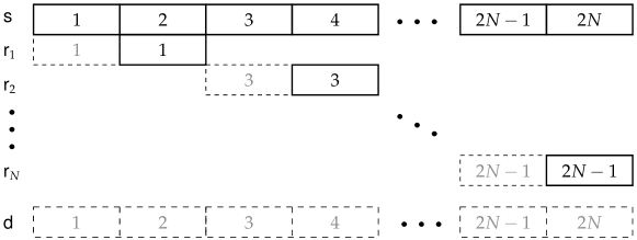
Figure 3: The NAF frame structure of an $N$-relay channel. Solid box for transmitted signal and dashed box for received signal.

In the multiple-relay case, a superframe of $N$ consecutive cooperation frames is defined, as shown in Fig. ​3. It is assumed that the channel is static during the transmission of the whole superframe (of $NT$ symbols). The $N$ relays take turns to cooperate with the source. Within each cooperation frame, the cooperation is in exactly the same manner as in the single-relay case. However, by allowing an encoding over the whole superframe, a diversity order of $N+1$ is achieved.

II-C Diversity-Multiplexing tradeoff (DMT)

Definition 1 (Multiplexing and diversity gain[10])

A coding scheme $\{\mathcal{C}({\mathsf{SNR}})\}$ is said to achieve multiplexing gain $r$ and diversity gain $d$ if

$$\lim_{{\mathsf{SNR}}\to\infty}\frac{R({\mathsf{SNR}})}{\log{\mathsf{SNR}}}=r\quad\textrm{and}\quad\lim_{{\mathsf{SNR}}\to\infty}\frac{\log P_{\textrm{e}}({\mathsf{SNR}})}{\log{\mathsf{SNR}}}=-d$$

where $R({\mathsf{SNR}})$ is the data rate measured by bits per channel use (PCU) and $P_{\textrm{e}}({\mathsf{SNR}})$ is the average error probability using the maximum likelihood (ML) decoder.

The optimal DMT of the single-antenna $N$-relay NAF channel

$$d_{\scriptscriptstyle\textrm{NAF}}(r)=(1-r)^{+}+N(1-2r)^{+}$$ (4)

is found in [6], where the achievability is proved by using a Gaussian random code with a sufficiently long block length.

III The NAF Scheme for MIMO Channel

In this section, we generalize the NAF protocol to the MIMO case, where each terminal is equipped with multiple antennas. The notation $(n_{\textrm{s}},n_{\textrm{r}},n_{\textrm{d}})$ will be used to denote a single-relay channel with $n_{\textrm{s}},n_{\textrm{r}}$ and $n_{\textrm{d}}$ antennas at the source, relay and destination. All matrix variables defined for a single-relay channel apply to a multiple-relay channel with an index $i$ denoting the $i^{\textrm{th}}$ relay.

III-A Signal Model

For convenience of demonstration, we only present the signal model of the single-relay channel. The extension to the multiple-relay case is straightforward.

III-A1 $n_{\textrm{r}}\leq n_{\textrm{s}}$

In the case $n_{\textrm{r}}\leq n_{\textrm{s}}$, a direct generalization of (2) is as follows :

$$\left\{\begin{aligned} {\boldsymbol{Y}}_{1}&=\sqrt{\pi_{1}{\mathsf{SNR}}}\,{\boldsymbol{F}}{\boldsymbol{X}}_{1}+{\boldsymbol{V}}_{1}\\ {\boldsymbol{Y}}_{r}&=\sqrt{\pi_{1}\rho\,{\mathsf{SNR}}}\,{\boldsymbol{H}}{\boldsymbol{X}}_{1}+{\boldsymbol{W}}\\ {\boldsymbol{Y}}_{2}&=\sqrt{\pi_{3}{\mathsf{SNR}}}\,{\boldsymbol{G}}({\boldsymbol{B}}{\boldsymbol{Y}}_{r})+\sqrt{\pi_{2}{\mathsf{SNR}}}\,{\boldsymbol{F}}{\boldsymbol{X}}_{2}+{\boldsymbol{V}}_{2}\end{aligned}\right.$$ (5)

where ${\boldsymbol{F}},{\boldsymbol{G}},{\boldsymbol{H}}$ are $n_{\textrm{d}}\times n_{\textrm{s}},n_{\textrm{d}}\times n_{\textrm{r}}$ and $n_{\textrm{r}}\times n_{\textrm{s}}$ independent matrices, respectively, with zero mean unit variance i.i.d. Gaussian entries; ${\boldsymbol{X}}_{i}$’s are $n_{\textrm{s}}\times\frac{T}{2}$ matrices with i.i.d. zero mean unit variance entries, representing the space-time signal from the source; ${\boldsymbol{V}}_{1},{\boldsymbol{V}}_{2}$ and ${\boldsymbol{W}}$ are independent AWGN matrices with normalized i.i.d. entries; the power allocation factors $\pi_{i}$’s satisfy $n_{\textrm{s}}(\pi_{1}+\pi_{2})+n_{\textrm{r}}\pi_{3}=2$ so that ${\mathsf{SNR}}$ denotes the received SNR per receive antenna at the destination; ${\boldsymbol{B}}$ is an $n_{\textrm{r}}\times n_{\textrm{r}}$ matrix equivalent to the “normalization factor” $b$ in the single-antenna case and is subject to the power constraint $\mathbb{E}\Bigl{\{}\left\|{{\boldsymbol{B}}{\boldsymbol{Y}}_{r}}\right\|^{2}_{\textrm{F}}\Bigr{\}}\leq\frac{T}{2}n_{\textrm{r}}$ which can be simplified to

$$\mathrm{Tr}\Bigl{\{}\left(\mathbf{I}+\pi_{1}\rho{\mathsf{SNR}}{\boldsymbol{H}}{{\boldsymbol{H}}}^{\scriptscriptstyle{\dagger}\!}\right){{\boldsymbol{B}}}^{\scriptscriptstyle{\dagger}\!}{\boldsymbol{B}}\Bigr{\}}\leq n_{\textrm{r}}.$$ (6)

Now, as in the single-antenna case, we obtain an equivalent single-user MIMO channel

$$\boldsymbol{\widetilde{y}}_{i}=\sqrt{{\mathsf{SNR}}}\boldsymbol{\widetilde{H}}\boldsymbol{\widetilde{x}}_{i}+{\boldsymbol{z}}_{i}\quad\textrm{for}\ i=1,\ldots,T/2$$ (7)

where $\boldsymbol{\widetilde{x}}_{i}={\bigl{[}{\boldsymbol{X}}_{1}[i]^{\scriptscriptstyle\mathsf{T}\!}\ {\boldsymbol{X}}_{2}[i]^{\scriptscriptstyle\mathsf{T}\!}\bigr{]}}^{\scriptscriptstyle\mathsf{T}\!}$ and $\boldsymbol{\widetilde{y}}_{i}={\bigl{[}{\boldsymbol{Y}}_{1}[i]^{\scriptscriptstyle\mathsf{T}\!}\ {\boldsymbol{Y}}_{2}[i]^{\scriptscriptstyle\mathsf{T}\!}\bigr{]}}^{\scriptscriptstyle\mathsf{T}\!}$ are the vectorized transmitted and received signals with ${\boldsymbol{M}}[i]$ denoting the $i^{\textrm{th}}$ column of the matrix ${\boldsymbol{M}}$; ${\boldsymbol{z}}_{i}\sim\mathcal{C}\mathcal{N}\!\left(0,\mathbf{I}\right)$ is the equivalent AWGN; the equivalent channel matrix $\boldsymbol{\widetilde{H}}$ is

$$\boldsymbol{\widetilde{H}}\triangleq\begin{bmatrix}\sqrt{\pi_{1}}{\boldsymbol{F}}&\boldsymbol{0}\\ \sqrt{\pi_{1}\pi_{3}}\,\boldsymbol{\Gamma}{\boldsymbol{P}}{\boldsymbol{H}}&\sqrt{\pi_{2}}\,\boldsymbol{\Gamma}{\boldsymbol{F}}\end{bmatrix}$$ (8)

with

$${\boldsymbol{P}}\triangleq\sqrt{{\mathsf{SNR}}}\,{\boldsymbol{G}}{\boldsymbol{B}}$$ (9)

and $\boldsymbol{\Gamma}$ being the whitening matrix satisfying $\left({\boldsymbol{\Gamma}}^{\scriptscriptstyle{\dagger}\!}\,\boldsymbol{\Gamma}\right)^{-1}=\left(\boldsymbol{\Gamma}{\boldsymbol{\Gamma}}^{\scriptscriptstyle{\dagger}\!}\right)^{-1}=\mathbf{I}+\pi_{3}{\boldsymbol{P}}{{\boldsymbol{P}}}^{\scriptscriptstyle{\dagger}\!}\triangleq\boldsymbol{\Sigma}$.

III-A2 $n_{\textrm{r}}>n_{\textrm{s}}$

With more antennas at the relay than at the source, the relay can do better than simple forwarding. In this case, the received signal at the relay is in the $n_{\textrm{s}}$-dimensional subspace generated by the $n_{\textrm{s}}$ eigenmodes of ${\boldsymbol{H}}$, represented by ${\boldsymbol{U}}_{\boldsymbol{H}}$ from the singular value decomposition ${\boldsymbol{H}}={\boldsymbol{U}}_{\boldsymbol{H}}\boldsymbol{\Sigma}_{{\boldsymbol{H}}}{{\boldsymbol{V}}}^{\scriptscriptstyle{\dagger}\!}_{\boldsymbol{H}}$. Since the relay-destination channel ${\boldsymbol{G}}$ is isotropic, it is of no use to forward the received signal in more than $n_{\textrm{r}}$ antennas (spatial directions).

However, by using only a subset of the antennas at the relay, we cannot obtain all the diversity gain provided by the channel ${\boldsymbol{G}}$. To exploit all the available diversity, we propose two schemes. The first scheme is the virtual $N$-relay scheme. Since no CSI is available at the transmitter and therefore no antenna combination is a priori better than the others, one solution is to use all the $\binom{n_{\textrm{r}}}{n_{\textrm{s}}}$ antenna combinations equally. Intuitively, the typical outage event is that all the antenna combinations are in deep fade, which implies that the channel ${\boldsymbol{G}}$ is also in outage. In this scheme, a superframe of $\binom{n_{\textrm{r}}}{n_{\textrm{s}}}$ cooperation frames is constructed. Within each cooperation frame, a different combination of $n_{\textrm{s}}$ antennas is used. The second scheme is the antenna selection scheme, which is used only when limited feedback from the destination to the relay is available. In this case, the destination tells the relay which antenna combination is optimal according to a given criterion (e.g., maximization of mutual information). With this scheme, maximum diversity gain is obtained without a superframe structure, which means a significant reduction of coding-decoding complexity.

As an example, let us consider a $(1,n_{\textrm{r}},1)$ relay channel with $n_{\textrm{r}}>1$. In this case, the received signal at the relay can be projected into a one-dimensional subspace. Consider a superframe of $n_{\textrm{r}}$ cooperation frames. In each cooperation frame, a different relay antenna is used. This scheme is virtually an $N$-relay single-antenna channel. The only difference is that the equivalent source-relay link, which is $\sqrt{\sum_{i}\left|h_{i}\right|^{2}}$ after the matched filter operation, is the same for the $N$ virtual relays. In this scheme, the achievable diversity order of the source-relay-destination link is $n_{\textrm{r}}$, since the channel is in outage only when $\sqrt{\sum_{i}\left|h_{i}\right|^{2}}$ is in deep fade or all the $n_{\textrm{r}}$ relay-destination links are in deep fade. When feedback is possible, the antenna selection scheme can be used. The difference from the first scheme is that only the antenna with maximum relay-destination channel gain (say, $\left|g_{\max}\right|\triangleq\displaystyle\max_{i=1\ldots n_{\textrm{r}}}\left\{\left|g_{i}\right|\right\}$) is used in the relaying phase. Therefore, only one cooperation frame is needed and the diversity order is also $n_{\textrm{r}}$.

III-B Optimal Diversity-Multiplexing Tradeoff: a Lower Bound

With the discussion above, considering the case $n_{\textrm{r}}\leq n_{\textrm{s}}$ is without loss of generality. In addition, since the destination is usually equipped with more antennas than the relays are in practice, we will restrict ourselves to the case $n_{\textrm{d}}\geq n_{\textrm{r}}$ hereafter. In the rest of this section, we study the optimal DMT of the MIMO NAF cooperative channel. Unlike the single-antenna case, a closed form expression of the DMT of the MIMO NAF channel is difficult to obtain, since the probability distribution (in the high SNR regime or not) of the eigenvalues of $\boldsymbol{\widetilde{H}}$ defined in (8) is unknown. In the following, we will derive a lower bound on the tradeoff, as a generalization of the DMT of the single-antenna NAF channel provided in [6]. To this end, we first study the DMT of a Rayleigh product channel.

III-B1 DMT of a Rayleigh Product Channel

Proposition 1

Let ${\boldsymbol{G}},{\boldsymbol{H}}$ be $n\times l,l\times m$ independent matrices with i.i.d. entries distributed as $\mathcal{C}\mathcal{N}\!\left(0,1\right)$. Assume that $m\geq l,n\geq l$ and define ${\boldsymbol{A}}\triangleq{\boldsymbol{G}}{\boldsymbol{H}},\Delta\triangleq\left|m-n\right|,q\triangleq\min\left\{m,n\right\}$, then the optimal DMT curve $d^{*}_{{\boldsymbol{A}}}(r)$ of the Rayleigh product channel, i.e., the channel defined by

$${\boldsymbol{y}}=\sqrt{\frac{{\mathsf{SNR}}}{l\cdot m}}{\boldsymbol{A}}{\boldsymbol{x}}+{\boldsymbol{z}}$$ (10)

with ${\boldsymbol{z}}\sim\mathcal{C}\mathcal{N}\!\left(0,1\right)$ being the AWGN is a piecewise-linear function connecting the points $(s,d^{*}_{{\boldsymbol{A}}}(s)),s=0,\ldots,l$, where

$$d^{*}_{{\boldsymbol{A}}}(s)=(l-s)(q-s)-\frac{1}{2}\left\lfloor\frac{\left[(l-\Delta-s)^{+}\right]^{2}}{2}\right\rfloor.$$ (11)

Proof:

See Appendix ​B. A more general result is given by [20], where a Rayleigh product channel is seen as a special case of the double scattering channels and the assumption $m\geq l,n\geq l$ is unnecessary. ∎

Remark 1

From proposition ​1, we note that

1. $d^{*}_{{\boldsymbol{A}}}(r)$ only depends on $\Delta$ and $q$, which means that interchanging $m$ and $n$ does not change $d^{*}_{{\boldsymbol{A}}}(r)$, which is obvious if we consider the fact that ${\boldsymbol{A}}{{\boldsymbol{A}}}^{\scriptscriptstyle{\dagger}\!}$ has the same eigenvalues as ${{\boldsymbol{A}}}^{\scriptscriptstyle{\dagger}\!}{\boldsymbol{A}}$;

2. $d^{*}_{{\boldsymbol{A}}}(s)$ is upper-bounded by $\bar{d}_{{\boldsymbol{A}}}(s)\triangleq\min\bigl{\{}d_{{\boldsymbol{H}}}(s),d_{{\boldsymbol{G}}}(s)\bigr{\}}=(l-s)(q-s)$ and coincides with it when $s\geq l-\Delta-1$;

3. when $\Delta\geq l-1$, $d^{*}_{{\boldsymbol{A}}}(s)=\bar{d}_{{\boldsymbol{A}}}(s),\forall s$. Without loss of generality, assume that $n\geq m$. Intuitively, by increasing $n$ and keeping $m$ unchanged, the diversity gain of the channel ${\boldsymbol{G}}$ is increasing and so is that of the product channel ${\boldsymbol{A}}$. When $n-m=l-1$, the best possible DMT for $q=m$ is achieved. With this $n$, the fading effect of ${\boldsymbol{G}}$ vanishes, since $d^{*}_{{\boldsymbol{A}}}(s)=d_{{\boldsymbol{H}}}(s)$. In other words, it is of no use to have $n>l+m-1$, for $m$ and $l$ fixed.

The optimal DMTs of a Rayleigh product channel for $l=2,3$ are illustrated in Fig. ​4. As indicated in remark 1, when $\Delta^{*}=1,2$ for $l=2,3$, the tradeoffs of the Rayleigh product channels are the same as those of the corresponding Rayleigh channels, i.e., the $2\times 2$ and $3\times 3$ Rayleigh channels.

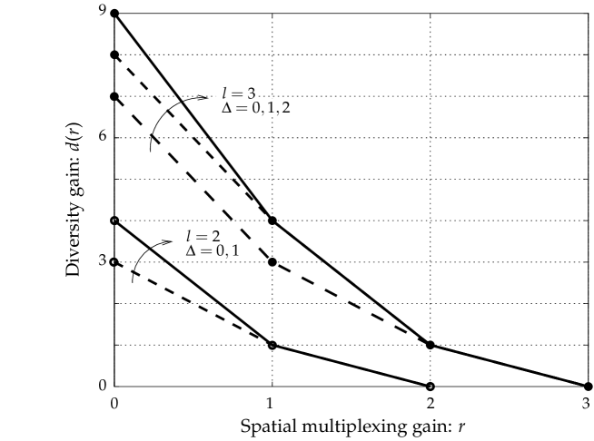
Figure 4: Optimal DMT: Rayleigh vs. Rayleigh product channel. $\min\{m,n\}=l=2,3$. $\Delta=0,\ldots,l-1$.

III-B2 DMT of a MIMO NAF Channel

Theorem 1

For a single-relay MIMO NAF channel (5), we have

$$d_{\scriptscriptstyle\textrm{NAF}}(r)\geq d_{{\boldsymbol{F}}}(r)+d_{{\boldsymbol{G}}{\boldsymbol{H}}}(2r)$$ (12)

where $d_{{\boldsymbol{F}}}(r)$ and $d_{{\boldsymbol{G}}{\boldsymbol{H}}}(r)$ are the optimal DMT of the fading channel ${\boldsymbol{F}}$ and the fading product channel ${\boldsymbol{G}}{\boldsymbol{H}}$, respectively.

Proof:

See Appendix ​C. ∎

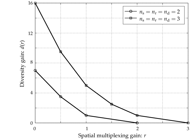
Figure 5: Lower bound on the optimal DMT: $n_{\textrm{s}}=n_{\textrm{r}}=n_{\textrm{d}}=2,3$.

The interpretation of (12) is as follows. First, since the transmitted signal passes through the source-destination link all the time, a diversity gain $d_{{\boldsymbol{F}}}(r)$ can be obtained. Then, due to the half duplex constraint, only half of the transmitted signal is protected by the source-relay-destination link, i.e., the channel defined by ${\boldsymbol{G}}{\boldsymbol{H}}$. Fig. 5 shows the lower bound (12) for a Rayleigh channel with $n_{\textrm{s}}=n_{\textrm{r}}=n_{\textrm{d}}=2$ and $3$.

This result of theorem 1 can be generalized to the $N$-relay case. Let ${\boldsymbol{G}}_{i}$ and ${\boldsymbol{H}}_{i}$ be channels related to the $i^{\textrm{th}}$ relay and be similarly defined as ${\boldsymbol{G}}$ and ${\boldsymbol{H}}$. The following theorem gives a lower bound on the optimal DMT of the $N$-relay MIMO NAF channel.

Theorem 2

For an $N$-relay MIMO NAF channel, we have

$$d_{\scriptscriptstyle\textrm{NAF}}(r)\geq d_{{\boldsymbol{F}}}(r)+\min_{\boldsymbol{\theta}:\sum_{i}\theta_{i}=1}\sum_{i=1}^{N}d_{{\boldsymbol{G}}_{i}{\boldsymbol{H}}_{i}}(2N\theta_{i}r).$$

In particular, when all the relays have the same number of antennas, we have

$$d_{\scriptscriptstyle\textrm{NAF}}(r)\geq d_{{\boldsymbol{F}}}(r)+Nd_{{\boldsymbol{G}}{\boldsymbol{H}}}(2r).$$ (13)

Proof:

See Appendix ​D. ∎

From (4), we see that the bound in (13) is actually the optimal tradeoff in the single-antenna case (i.e., $n_{\textrm{s}}=n_{\textrm{r}}=n_{\textrm{d}}=1$).

Corollary 1

Let $d_{i}\triangleq\min\bigl{\{}d_{{\boldsymbol{G}}_{i}}(0),d_{{\boldsymbol{H}}_{i}}(0)\bigr{\}},i=1,\ldots,N$. Then, we have

$$d_{{\boldsymbol{F}}}(0)+\sum_{i=1}^{N}d_{i}(0)\geq d_{\scriptscriptstyle\textrm{NAF}}(0)\geq d_{{\boldsymbol{F}}}(0)+\sum_{i=1}^{N}d_{{\boldsymbol{G}}_{i}{\boldsymbol{H}}_{i}}(0).$$ (14)

If all the channels are Rayleigh distributed and $\left|m-n\right|\geq l_{i}-1,\forall i$, then, we have

$$d_{\scriptscriptstyle\textrm{NAF}}(0)=d_{{\boldsymbol{F}}}(0)+\sum_{i=1}^{N}d_{i}(0).$$ (15)

Proof:

See Appendix ​D. ∎

IV Optimal Codes Design Criteria

In this section, we will derive design criteria for a family of short codes to achieve the optimal DMT of an $N$-relay MIMO NAF channel.

IV-A A General Result

Let us first define the “good” code mentioned in section I.

Definition 2 (Rate-$n$ NVD code)

Let $\mathcal{A}$ be an alphabet that is scalably dense, i.e., for $0\leq r\leq n$

$$\left|\mathcal{A}({\mathsf{SNR}})\right|\doteq{\mathsf{SNR}}^{\frac{r}{n}}\quad\textrm{and}$$

$$a\in\mathcal{A}({\mathsf{SNR}})\Rightarrow\left|a\right|^{2}\ \dot{\leq}\,{\mathsf{SNR}}^{\frac{r}{n}}$$

Then, an $n_{\textrm{T}}\times n_{\textrm{T}}$ space-time code $\mathcal{X}$ is called a rate-$n$ NVD code if it

1. is $\mathcal{A}$-linear;

2. transmits on average $n$ symbols PCU from the signal constellation $\mathcal{A}$;

3. has the non-vanishing determinant (NVD) property.

The following theorem is fundamental to our construction.

Theorem 3

For any linear block fading channel

$${\boldsymbol{y}}=\sqrt{{\mathsf{SNR}}}{\boldsymbol{H}}{\boldsymbol{x}}+{\boldsymbol{z}}$$

where ${\boldsymbol{H}}$ is an $n_{\textrm{R}}\times n_{\textrm{T}}$ channel and ${\boldsymbol{z}}\sim\mathcal{C}\mathcal{N}\!\left(0,\mathbf{I}\right)$ is the AWGN, the achievable DMT of a rate-$n$ NVD code $\mathcal{X}$ satisfies

$$d_{\mathcal{X}}(r)\geq d_{\textrm{out}}\left(\frac{q}{n}r\right)$$ (16)

where $q\triangleq\min\{n_{\textrm{R}},n_{\textrm{T}}\}$ and $d_{\textrm{out}}(r)$ is the outage upper bound of the DMT for the channel ${\boldsymbol{H}}$.

Proof:

See Appendix ​E. ∎

In particular, for a full rate code ($n=q$), the upper bound $d_{\textrm{out}}(r)$ is achievable. This theorem implies that the NVD property is fundamental for $\mathcal{X}$ to achieve all the diversity gain $d$, for any linear fading channel. For a given diversity gain $d$, the achievable multiplexing gain $r$ of such $\mathcal{X}$ is a shrunk version of $r_{\textrm{out}}(d)$, the best that we can have for channel ${\boldsymbol{H}}$.

One of the consequences of theorem ​3 is the possibility of constructing optimal codes (in terms of the DMT) based on the NVD criteria for some channels. For example, we can get an equivalent MIMO space-time model for the single-antenna fast fading channel (also called a Gaussian parallel channel) as

$${\boldsymbol{Y}}=\mathrm{diag}\left(h_{1},\ldots,h_{N}\right){\boldsymbol{X}}+{\boldsymbol{Z}}$$ (17)

with ${\boldsymbol{X}},{\boldsymbol{Y}}$ and ${\boldsymbol{Z}}$ diagonal $N\times N$ matrices. The best code that we can have is a rate-$1$ NVD code $\mathcal{X}$ due to the diagonal constraint. According to theorem ​3, we have $d_{\mathcal{X}}(r)\geq d_{\textrm{out}}(Nr)$ with $d_{\textrm{out}}(r)$ the DMT of (17) without the diagonal constraint. In fact, we can verify that $d_{\textrm{out}}(Nr)$ coincides with the DMT of the fast fading channel. The NVD criterion includes the product distance criterion since the determinant of a diagonal matrix is the product of the diagonal entries. In addition, it implies that the product distance should be non-vanishing as the constellation size increases.

Note that another such general result as theorem 3, has been derived independently in [14]. In [11], the NVD property is derived from the mismatched eigenvalue bound (worst case rotation) while the results in [14] are derived using the worst case codeword error probability, which is effectively the same thing as the worst case rotation. Theorem 3 is a generalization of the result in [11] (for the full rate codes) to a rate-$n$ code. This result is more adapted to the algebraic construction of explicit codes for the relay channel.

IV-B Design Criteria

With theorem ​3, we are ready to give out the design criteria of the optimal codes for the NAF cooperative channel. The following theorem states the main result of our work.

Theorem 4

Let $\mathcal{X}$ be a rate-($2n_{\textrm{s}}$) NVD block diagonal code, i.e.,

$${\boldsymbol{X}}=\begin{bmatrix}\boldsymbol{\Xi}_{1}&\cdots&0\\ \vdots&\ddots&\vdots\\ 0&\cdots&\boldsymbol{\Xi}_{N}\end{bmatrix},\quad\forall{\boldsymbol{X}}\in\mathcal{X}$$

where $\boldsymbol{\Xi}_{i}$’s are $2n_{\textrm{s}}\times 2n_{\textrm{s}}$ matrices. Now consider an equivalent code $\mathcal{C}$ whose codewords are in the form

$${\boldsymbol{C}}=\begin{bmatrix}{\boldsymbol{C}}_{1}&\ldots&{\boldsymbol{C}}_{N}\end{bmatrix}$$

with

$${\boldsymbol{C}}_{i}\triangleq\begin{bmatrix}\boldsymbol{\Xi}_{i}\left(1\!:\!n_{\textrm{s}},1\!:\!2n_{\textrm{s}}\right)&\boldsymbol{\Xi}_{i}\left(n_{\textrm{s}}\!+\!1\!:\!2n_{\textrm{s}},1\!:\!2n_{\textrm{s}}\right)\end{bmatrix}.$$

Then, $\mathcal{C}$ achieves the optimal DMT of the $N$-relay MIMO NAF channel with $n_{\textrm{s}}$ transmit antennas at the source, by transmitting ${\boldsymbol{C}}_{i}$ in the $i^{\textrm{th}}$ cooperation frame. The code $\mathcal{C}$ is of length $4Nn_{\textrm{s}}$.

Proof:

See Appendix ​F. ∎

In section III, a lower bound on the optimal DMT of a MIMO NAF channel is derived. Here, theorem 4 shows that the exact optimal tradeoff can always be achieved by a code $\mathcal{C}$, even though we cannot obtain its closed form expression.

V A Unified Construction Framework

V-A Notations and Assumptions

We assume that the modulation used by the source is either a QAM or a HEX modulation. The fields representing the modulated symbols will be either $\mathbb{Q}(i)$ or $\mathbb{Q}(j)$. We denote it as $\mathbb{P}$. For each algebraic number field $\mathbb{K}$, the ring of integers is denoted $\mathcal{O}_{\mathbb{K}}$.

V-B Behavior of the Codewords

We recall that a codeword ${\boldsymbol{X}}$ is represented by a block diagonal matrix

$${\boldsymbol{X}}=\begin{bmatrix}\boldsymbol{\Xi}_{1}&\cdots&0\\ \vdots&\ddots&\vdots\\ 0&\cdots&\boldsymbol{\Xi}_{N}\end{bmatrix}$$ (18)

with $\boldsymbol{\Xi}_{i},\,\,i=1,\ldots,N$ being a square $2n_{\textrm{s}}\times 2n_{\textrm{s}}$ matrix. The criteria to fulfill are the following :

1. full rate : the number of QAM or HEX independent symbols in a codeword is equal to $N\cdot(2n_{\textrm{s}})^{2}$ corresponding to a multiplexing gain of $n_{\textrm{s}}$ symbols PCU;

2. full rank :

   $$\min_{{{\boldsymbol{X}}_{1},{\boldsymbol{X}}_{2}\in\mathcal{C}}\atop{{\boldsymbol{X}}_{1}\neq{\boldsymbol{X}}_{2}}}\textrm{rank}({\boldsymbol{X}}_{1}-{\boldsymbol{X}}_{2})=N\cdot(2n_{\textrm{s}});$$ (19)

3. non-vanishing determinant :

   $$\min_{{{\boldsymbol{X}}_{1},{\boldsymbol{X}}_{2}\in\mathcal{C}}\atop{{\boldsymbol{X}}_{1}\neq{\boldsymbol{X}}_{2}}}\left|\det({\boldsymbol{X}}_{1}-{\boldsymbol{X}}_{2})\right|^{2}\geq\kappa$$ (20)

   with $\kappa$ being some strictly positive constant.

V-C Codes Construction

We use the same methods as in [13]. Some particular cases can be found in [15, 12]. The main difference is in the choice of the base field $\mathbb{F}$. In [13], this base field was equal to $\mathbb{P}$. Here, we choose a Galois extension of $\mathbb{P}$ with degree $N$ and denote $\tau_{i},\,\,i=1,\ldots,N$ the elements of its Galois group $\mathcal{G}al_{\mathbb{F}/\mathbb{P}}$. Now, we construct a cyclic algebra whose center is $\mathbb{F}$. We need a cyclic extension over $\mathbb{F}$ of degree $2n_{\textrm{s}}$. We denote it $\mathbb{K}$. The generator of its Galois group is $\sigma$. The code construction needs two steps.

1. Construction of the cyclic algebra

   $$\mathcal{A}=\left\{\left.\sum_{i=0}^{2n_{\textrm{s}}-1}z_{i}\cdot e^{i}\ \right|z_{i}\in\mathbb{K}\right\}$$ (21)

   such that $e^{2n_{\textrm{s}}}=\gamma\in\mathbb{F}$ and $z_{i}\cdot e=e\cdot\sigma\left(z_{i}\right)$. In the matrix representation, we have

   $$e=\begin{bmatrix}0&1&0&\cdots&0\\ 0&0&1&\ddots&\vdots\\ \vdots&&\ddots&\ddots&0\\ 0&\vdots&&\ddots&1\\ \gamma&0&\cdots&&0\end{bmatrix}$$

   and $z_{i}=\textrm{diag}\left(z_{i},\sigma\left(z_{i}\right),\sigma^{2}\left(z_{i}\right),\ldots,\sigma^{2n_{\textrm{s}}-1}\left(z_{i}\right)\right)$.

2. Application of the embeddings of $\mathbb{F}/\mathbb{P}$.

In terms of matrices, we construct, in step 1, the square $2n_{\textrm{s}}\times 2n_{\textrm{s}}$ matrix $\boldsymbol{\Xi}$. Then, by applying the embeddings of $\mathbb{F}/\mathbb{P}$, the codeword is

$${\boldsymbol{X}}=\begin{bmatrix}\tau_{1}(\boldsymbol{\Xi})&\cdots&0\\ \vdots&\ddots&\vdots\\ 0&\cdots&\tau_{N}(\boldsymbol{\Xi})\end{bmatrix}$$ (22)

where we can identify $\tau_{i}(\boldsymbol{\Xi})=\boldsymbol{\Xi}_{i}$ from (18). As usual, we restrict the information symbols to be in $\mathcal{O}_{\mathbb{P}}$, that is, $\mathbb{Z}[i]$ (QAM symbols) or $\mathbb{Z}[j]$ (HEX symbols). So, instead of being in $\mathbb{F}$, we will be in $\mathcal{O}_{\mathbb{F}}$ and in the same way, we will be in $\mathcal{O}_{\mathbb{K}}$ instead of $\mathbb{K}$. The infinite space-time code is defined as being the set of all matrices

$$\mathcal{C}=\left\{{\boldsymbol{X}}=\begin{bmatrix}\tau_{1}\left(\displaystyle\sum_{i=0}^{2n_{\textrm{s}}-1}z_{i}e^{i}\right)&\cdots&0\\ \vdots&\ddots&\vdots\\ 0&\cdots&\tau_{N}\left(\displaystyle\sum_{i=0}^{2n_{\textrm{s}}-1}z_{i}e^{i}\right)\end{bmatrix}\right\}.$$ (23)

V-D Codes Properties

Lemma 1

The code $\mathcal{C}$ of (23) is full rate.

Proof:

In the submatrix $\boldsymbol{\Xi}$, there are $2n_{\textrm{s}}$ independent elements of $\mathcal{O}_{\mathbb{K}}$. Each element in $\mathcal{O}_{\mathbb{K}}$ is a linear combination of $2n_{\textrm{s}}$ elements of $\mathcal{O}_{\mathbb{F}}$. Finally, each element of $\mathcal{O}_{\mathbb{F}}$ is a linear combination of $N$ QAM or HEX symbols. So, each codeword ${\boldsymbol{X}}$ is a linear combination of $N\cdot(2n_{\textrm{s}})^{2}$ QAM or HEX symbols. ∎

Lemma 2

If $\gamma,\gamma^{2},\ldots,\gamma^{2n_{s}-1}\notin N_{\mathbb{K}/\mathbb{F}}(\mathbb{K})$, then the code $\mathcal{C}$ is full rank.

Proof:

In [16], it is proved that if $\gamma,\gamma^{2},\ldots,\gamma^{2n_{s}-1}\notin N_{\mathbb{K}/\mathbb{F}}(\mathbb{K})$, then the cyclic algebra $\mathcal{A}$ is a division algebra (each element has an inverse). ∎

Lemma 3

If $\gamma,\gamma^{2},\ldots,\gamma^{2n_{s}-1}\notin N_{\mathbb{K}/\mathbb{F}}(\mathbb{K})$, then the code $\mathcal{C}$ has a non-vanishing determinant, more precisely

$$\delta_{\min}\triangleq\min_{{{\boldsymbol{X}}\in\mathcal{C}}\atop{{\boldsymbol{X}}\neq 0}}\left|\det{\boldsymbol{X}}\right|^{2}\in\mathbb{Z}^{+}\!\setminus\!\{0\}\geq 1.$$

Proof:

Because of the structure of ${\boldsymbol{X}}$, its determinant is

$$\det{\boldsymbol{X}}=\prod_{i=1}^{N}\det\tau_{i}(\boldsymbol{\Xi})=\prod_{i=1}^{N}\tau_{i}\left(\det(\boldsymbol{\Xi})\right).$$

But, $\det(\boldsymbol{\Xi})$ is the reduced norm of $\sum_{i=0}^{2n_{\textrm{s}}-1}z_{i}e^{i}$ thus it belongs to $\mathcal{O}_{\mathbb{F}}$. So,

$$\prod_{i=1}^{N}\tau_{i}\left(\det(\boldsymbol{\Xi})\right)=N_{\mathbb{F}/\mathbb{P}}\left(\det(\boldsymbol{\Xi})\right)\in\mathcal{O}_{\mathbb{P}}$$

with $\mathcal{O}_{\mathbb{P}}=\mathbb{Z}[i]$ or $\mathcal{O}_{\mathbb{P}}=\mathbb{Z}[j]$. Since $\det({\boldsymbol{X}})\neq 0$ unless ${\boldsymbol{X}}=\boldsymbol{0}$, we get $\delta_{\min}\geq 1$. ∎

Finally, the following result is derived.

Theorem 5

The code $\mathcal{C}$ of (23) with $z_{i}\in\mathcal{O}_{\mathbb{K}}$ or a subspace of $\mathcal{O}_{\mathbb{K}}$ (which will be in the following an ideal of $\mathcal{O}_{\mathbb{K}}$) achieves the DMT of the MIMO NAF cooperative channel when $N$ is the number of relays and $n_{\textrm{s}}$ is the number of antennas at the source.

Proof:

The proof is straightforward and uses the results of the $3$ above lemmas. ∎

V-E Shaping

As in [12, 13], we may be interested in constructing codes that achieve the DMT and that behave well in terms of error probability even for small alphabets such as QPSK (4QAM). In that case, we add another constraint to our codes design, the shaping factor. This new constraint implies that $\left|\gamma\right|=1$. Moreover, as in [12, 13], the linear transform that sends the vector composed by the $N\cdot{(2n_{\textrm{s}})}^{2}$ QAM or HEX information symbols to $\textrm{vec}({\boldsymbol{X}})$ has to be unitary. The following examples will illustrate this claim.

VI Some Examples

We give some examples of the code construction. Our code for an $N$-relay $k$-antenna channel is denoted $\mathcal{C}_{N,k}$.

VI-A The Golden Code [12] is Optimal for the Single-Relay Single-Antenna NAF Channel

In the case of single-relay single-antenna channel, the codewords are $2\times 2$ matrices. Because the Golden code satisfies to all the criteria of subsection V-B, it achieves the optimal DMT of the channel.

VI-B Two Relays, Single Antenna

Optimal codes for the case $N>1$ relays cannot be found in the literature.

For the $2$-relay case, we propose the following code. Codewords are block diagonal matrices with $2$ blocks. Each block is a $2\times 2$ matrix. Let $\mathbb{P}=\mathbb{Q}(i)$ and $\mathbb{F}=\mathbb{Q}\left(\zeta_{8}\right)$ with $\zeta_{8}=e^{\frac{i\pi}{4}}$ be an extension of $\mathbb{Q}(i)$ of degree $2$. We choose $\mathbb{K}=\mathbb{F}\left(\sqrt{5}\right)=\mathbb{Q}\left(\zeta_{8},\sqrt{5}\right)$. In fact, we try to construct the Golden code on the base field $\mathbb{Q}\left(\zeta_{8}\right)$ instead of the base field $\mathbb{Q}(i)$. Moreover, the number $\gamma$ is no more equal to $i$ because $i$ is a norm in $\mathbb{Q}\left(\zeta_{8}\right)$ ($i=N_{\mathbb{K}/\mathbb{F}}\left(\zeta_{8}\right)$). We choose here, in order to preserve the shaping of the code, $\gamma=\zeta_{8}$. We prove in appendix G that $\zeta_{8}\notin N_{\mathbb{K}/\mathbb{F}}(\mathbb{K})$ and thus that this code satisfies to the full rank and the NVD conditions. Such a code uses $8$ QAM symbols. Let $\theta=\frac{1+\sqrt{5}}{2}$, $\gamma=\zeta_{8}$ and $\sigma:\theta\mapsto\bar{\theta}=\frac{1-\sqrt{5}}{2}$. The ring of integers of $\mathbb{K}$ is $\mathcal{O}_{\mathbb{K}}=\left\{a+b\theta\mid a,b\in\mathbb{Z}\left[\zeta_{8}\right]\right\}$. Let $\alpha=1+i-i\theta$ and $\bar{\alpha}=1+i-i\bar{\theta}$. Codewords are given by

$${\boldsymbol{X}}=\begin{bmatrix}\boldsymbol{\Xi}&\boldsymbol{0}\\ \boldsymbol{0}&\tau(\boldsymbol{\Xi})\end{bmatrix}$$

with

$$\boldsymbol{\Xi}=\frac{1}{\sqrt{5}}\begin{bmatrix}\alpha\cdot\left(s_{1}+s_{2}\zeta_{8}+s_{3}\theta+s_{4}\zeta_{8}\theta\right)&\alpha\cdot\left(s_{5}+s_{6}\zeta_{8}+s_{7}\theta+s_{8}\zeta_{8}\theta\right)\\ \zeta_{8}\bar{\alpha}\cdot\left(s_{5}+s_{6}\zeta_{8}+s_{7}\bar{\theta}+s_{8}\zeta_{8}\bar{\theta}\right)&\bar{\alpha}\cdot\left(s_{1}+s_{2}\zeta_{8}+s_{3}\bar{\theta}+s_{4}\zeta_{8}\bar{\theta}\right)\end{bmatrix}$$

and $\tau$ changes $\zeta_{8}$ into $-\zeta_{8}$.

VI-C Four Relays, Single Antenna

The generalization to $N=4$ relays is straightforward. Codewords are block diagonal matrices with $4$ blocks. Each block is a $2\times 2$ matrix. Let $\mathbb{P}=\mathbb{Q}(i)$ and $\mathbb{F}=\mathbb{Q}\left(\zeta_{16}\right)$ with $\zeta_{16}=e^{\frac{i\pi}{8}}$ be an extension of $\mathbb{Q}(i)$ of degree $4$. We choose $\mathbb{K}=\mathbb{F}\left(\sqrt{5}\right)=\mathbb{Q}\left(\zeta_{16},\sqrt{5}\right)$. We choose here, in order to preserve the shaping of the code, $\gamma=\zeta_{16}$. We prove in appendix H that $\zeta_{16}\notin N_{\mathbb{K}/\mathbb{F}}(\mathbb{K})$ and thus that this code satisfies to the full rank and the NVD conditions.

VI-D Single Relay, Two Antennas

Since $n_{s}=2$ and $N=1$, we need a code whose codewords are represented by a $4\times 4$ NVD space-time code. The $4\times 4$ Perfect code of [13] satisfies to all criteria.

VI-E Two Relays, Two Antennas

We assume here that the source uses $2$ antennas and that there are $2$ relays. The idea is to construct a $4\times 4$ Perfect code not on the base field $\mathbb{F}=\mathbb{Q}(i)$ as it is the case in [13], but on the base field $\mathbb{F}=\mathbb{Q}\left(\zeta_{8}\right)$. Thus, a rate-$2$ NVD code can be constructed as follows:

• Take $\mathbb{F}=\mathbb{Q}\left(\zeta_{8}\right)$.

• Choose $\mathbb{K}=\mathbb{F}\left(2\cos\left(\frac{2\pi}{15}\right)\right)=\mathbb{Q}\left(\zeta_{8},2\cos\left(\frac{2\pi}{15}\right)\right)$.

• Finally, take $\gamma=\zeta_{8}$.

We can show, in the same way as in appendix G, that if $\zeta_{8}$ was a norm in $\mathbb{Q}\left(\zeta_{8},2\cos\left(\frac{2\pi}{15}\right)\right)$, then $i$ must be a norm in $\mathbb{Q}\left(i,2\cos\left(\frac{2\pi}{15}\right)\right)$ which contradicts the results of [13]. The case of $\gamma^{2}$ is obvious since $\gamma^{2}=i$. Now, in order to prove that $\gamma^{3}=i\zeta_{8}$ is not a norm, it is enough to replace $\zeta_{8}$ by $i\zeta_{8}$ and $z$ by $y$ in appendix G and show in the same way that if $i\zeta_{8}$ was a norm in $\mathbb{Q}\left(\zeta_{8},2\cos\left(\frac{2\pi}{15}\right)\right)$, then $i$ must be a norm in $\mathbb{Q}\left(i,2\cos\left(\frac{2\pi}{15}\right)\right)$.

VII Numerical Results

In this section, we provide the simulation results on the performance of some of the codes proposed in section VI. The performance is measured by the frame error rate (FER) vs. receive SNR per bit. For simplicity, we set the power allocation factors $\pi_{1}=2\pi_{2}=2\pi_{3}$ for all the scenarios that we considered in this section. An optimization on the $\pi_{i}$’s in function of $\rho$ and ${\mathsf{SNR}}$ can improve the performance. However, this kind of optimization is out of the scope of this paper and will not be considered here. The transmitted signal constellation is $4$- and $64$-QAM. The geometric gain $\rho$ varies from $0$ to $20$ dB.

VII-A Single-Antenna Channel

Fig. 7 shows the performance of the Golden code on the single-relay single-antenna channel. The performance of the channel without relay is also shown in the figures. In this case, the frame length is $4$ symbols. Compared to the non-cooperative case, the Golden code achieves diversity $2$. For $4$-QAM, a gain of $12.5$ dB (resp. $13.8,14.3$ and $14.8$ dB) is observed for $\rho=0$ dB (resp. $5,10$ and $20$ dB) at $\textrm{FER}=10^{-4}$. First of all, note that in the low SNR regime, the non-cooperative channel is better than the cooperative channel. This is due to the error cumulation (at the relay) which is more significant than the diversity gain provided by the relay in this regime. Then, we see that the difference between $\rho=10$ dB and $\rho=20$ dB is negligible, which means that a geometric gain of $10$ dB is enough to achieve the (almost) best performance of the Golden code. In practice, it is often possible to find this kind of “helping agent” (with a geometric gain of $10$ dB). When we increase the spectral efficiency ($64$-QAM), same phenomena can be observed except that the gain of the relay channel is reduced. Still, a gain of $6.3$ and $9.5$ dB can be obtained at $\textrm{FER}=10^{-4}$ for $\rho=0$ and $20$ dB.

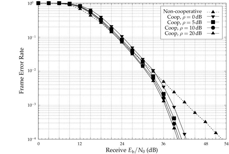
(b) $64$-QAM

Figure 8: Four-relay single-antenna NAF channel, Rayleigh fading, $\mathcal{C}_{4,1}$.

The performance of $\mathcal{C}_{4,1}$ on the four-relay single-antenna channel is illustrated in Fig. 8. The frame length is $16$. For $\rho=20$ dB, a gain of $21$ dB (resp. $12.8$ dB) at $\textrm{FER}=10^{-4}$ is obtained with $4$-QAM (resp. $64$-QAM).

VII-B Multi-Antenna Channel

VII-B1 A $(1,2,1)$-Relay Channel

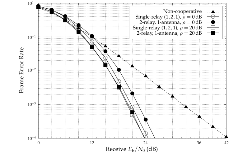
Figure 9: Single-relay $(1,2,1)$ NAF channel vs. two-relay single-antenna NAF channel, Rayleigh fading, $\mathcal{C}_{2,1}$ with $4$-QAM.

As an example for the case $n_{r}>n_{s}$, we consider the $(1,2,1)$ channel. Here, we use the virtual $N$-relay scheme with $N=2$. As discussed in section III-A2, the diversity order of this scheme is comparable to the $2$-relay single-antenna channel. To compare these two channels, we use the same code $\mathcal{C}_{2,1}$. The performance is shown in Fig. 9. As compared to the $2$-relay single-antenna channel, the $(1,2,1)$ channel has a gain of $1.5$ dB at $\textrm{FER}=10^{-4}$ with $\rho=0$ dB. With $\rho=20$ dB, the two channels have essentially the same performance. In fact, the inter-relay cooperation in the virtual two-relay channel improves the receive SNR ($3$ dB) of the source-relay channel with antenna combining. Thus, the geometric gain $\rho$ is increased effectively. However, as stated before, the global performace is not sensitive to $\rho$ for large $\rho$’s. This is why there is a gain only with small $\rho$’s.

VII-B2 A $(2,2,2)$-Relay Channel

In the case of $n_{s}\geq n_{r}$, we consider a single-relay channel with two antennas at each terminal. The code $\mathcal{C}_{1,2}$ is actually the $4\times 4$ Perfect code. For the non-cooperative scenario, we take the same code for fairness of comparison. More precisely, the non-cooperative channel we consider here is equivalent to a cooperative channel with $\pi_{3}=0$ and $\pi_{1}=\pi_{2}$. As shown in Fig. ​10, the gain of the cooperative channel over the non-cooperative channel is much less significant in the SNRs of interest. This is because the diversity order of the Perfect code in the two-antenna non-cooperative channel is already $4$ and a diversity gain does not play an important role in the scope of interest. Note that at $\textrm{FER}=10^{-5}$, the gain of the cooperative channel with $\rho=0$ dB over the non-cooperative channel is $2$ dB for $4$-QAM and $3$ dB for $64$-QAM. Also note that the difference between different $\rho$’s is within $1$ dB.

VII-B3 A $(2,2,2)$-Relay Channel with Shadowing

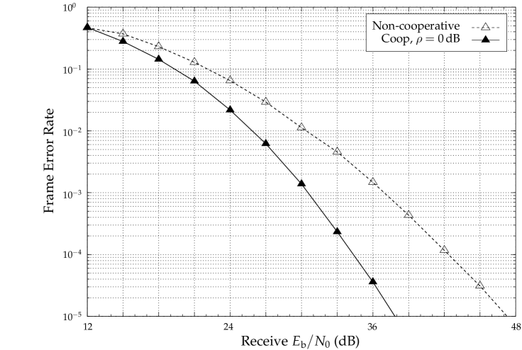
Figure 11: Single-relay $(2,2,2)$ NAF channel, Rayleigh fading, log-normal shadowing with variance $7$dB, $4$-QAM, $4\times 4$ Perfect code.

In this scenario, we consider the shadowing effect of a wireless channel. Assume that each link between terminals is shadowed. Mathematically, the channel matrix is multiplied by a random scalar variable, the shadowing coefficient. Suppose that this variable is log-normal distributed of variance $7$ dB[17] and that the shadowing is independent for different links. Fig. 11 shows the performance of the cooperative channel with the use of $\mathcal{C}_{1,2}$ ($4$-QAM) at $\rho=0$ dB, as compared to the non-cooperative channel. FER is the averaged frame error rate on the channel fading and the shadowing. As shown in Fig. ​11, the slope of the FER-SNR curve of the non-cooperative channel is reduced as compared to the non-shadowing case, in the scale of interest. Since the shadowing is independent between different links, the cooperative channel mitigates the shadowing effect and we get a larger gain over the non-cooperative channel than in the non-shadowing case (Fig. ​10(a)). At $\textrm{FER}=10^{-4}$, this gain is $8$ dB, in contrast to $1.2$ dB in the non-shadowing case (Fig. ​10(a)).

VIII Conclusion and Future Work

In this paper, a half-duplex MIMO amplify-and-forward cooperative diversity scheme is studied. We derived the optimal diversity-multiplexing tradeoff of a MIMO Rayleigh product channel, from which we obtain a lower bound on the optimal diversity-multiplexing tradeoff of a MIMO NAF cooperative channel. Moreover, we established a lower and upper bound on the maximum diversity order of the proposed MIMO NAF channel and showed that they coincide when the numbers of antenna satisfy certain conditions. Based on the non-vanishing determinant criterion, we constructed a family of short space-time block codes that achieve the DMT of our MIMO NAF model. Our construction is systematic and applies to a system with arbitrary number of relays and arbitrary number of antennas. Numerical results on some explicit example codes revealed that significant gain in terms of SNR can be obtained even with some non-optimized parameters. This gain is much more important in the single-antenna case than in the MIMO case. Fortunately, in reality, it is also the case that we need cooperative diversity only when local antenna array is not available.

Nevertheless, it still remains two important open problems to solve :

1. optimization of the power allocation factors: Based on the statistical knowledge of the channel (notably $\rho$), how to choose the factors $\pi_{i}$’s in order to optimize the code performance according to certain criteria? We set $\pi_{1}=2\pi_{2}=2\pi_{3}$ for simplicity. It is clear that the optimal DMT is independent of these parameters. However, in practice, for different $\rho$ and ${\mathsf{SNR}}$, the factor $\pi_{i}$’s are significant for the performance (e.g., the error rate performance). How to analyze the impact theoretically is an interesting future work;

2. optimization of the matrix ${\boldsymbol{B}}$: we set ${\boldsymbol{B}}$ to be identity matrix and derived the lower bound (12). Based on the receiver CSI at the relay, is there an optimal matrix ${\boldsymbol{B}}$ that gives a better DMT than the lower bound (12)? This problem is independent of the code we use. Solving this problem may lead to solution for the exact DMT of the MIMO NAF channel.

Appendix A Preliminaries to the Proofs

For sake of simplicity, we use the dot (in)equalites throughout the proofs to describe the behavior of different quantities in the high SNR regime. More precisely,

• for probability related quantities,

  $$p_{1}\doteq p_{2}\quad\textrm{means}\quad\lim_{{\mathsf{SNR}}\to\infty}\frac{\log p_{1}}{\log{\mathsf{SNR}}}=\lim_{{\mathsf{SNR}}\to\infty}\frac{\log p_{2}}{\log{\mathsf{SNR}}};$$

• for mutual information related quantities,

  $$\mathcal{I}_{1}\doteq\mathcal{I}_{2}\quad\textrm{means}\quad\lim_{{\mathsf{SNR}}\to\infty}\frac{\mathcal{I}_{1}}{\log{\mathsf{SNR}}}=\lim_{{\mathsf{SNR}}\to\infty}\frac{\mathcal{I}_{2}}{\log{\mathsf{SNR}}};$$

• for sets,

  $$\mathcal{S}_{1}\doteq\mathcal{S}_{2}\quad\textrm{means}\quad\textrm{Prob}\left\{s\in\mathcal{S}_{1}\right\}\doteq\textrm{Prob}\left\{s\in\mathcal{S}_{2}\right\}.$$

  $\ \dot{\geq}\,$, $\ \dot{\leq}\,$, $\ \dot{\supseteq}\,$ and $\ \dot{\subseteq}\,$ are similarly defined.

Definition 3 (Exponential order[6])

For any nonnegative random variable $x$, the exponential order is defined as

$$\xi \triangleq -\lim_{{\mathsf{SNR}}\to\infty}\frac{\log{x}}{\log{\mathsf{SNR}}}.$$ (24)

We denote $x\doteq{\mathsf{SNR}}^{-\xi}$.

Lemma 4

Let $X$ be a $\chi^{2}$-distribution random variable with $2t$ degrees of freedom, the probability density function of its exponential order $\xi$ satisfies

$$p_{\xi}\doteq\left\{\begin{IEEEeqnarraybox}[]{[}][c]{l^{\prime}s}{\mathsf{SNR}}^{-\infty},&for$\xi<0$;\\ {\mathsf{SNR}}^{-\xi t},&for$\xi\geq 0$.\end{IEEEeqnarraybox}\right.$$

Let $\mathcal{S}$ be a certain set, $\xi_{i}$’s be independent random variables with $\xi_{i}\sim\chi^{2}_{2t_{i}}$, and $P_{\mathcal{S}}\triangleq\textrm{Prob}\Big{\{}(\xi_{1},\ldots,\xi_{N})\in\mathcal{S}\Big{\}}$, then we have

$$P_{\mathcal{S}}\doteq{\mathsf{SNR}}^{-d}\quad\textrm{with}\quad d=\inf_{(\xi_{1}\ldots{\xi_{N}})\in\mathcal{S}^{+}}\sum_{i=1}^{N}t_{i}\xi_{i}$$

where $\mathcal{S}^{+}=\mathcal{S}\bigcap\mathbb{R}^{N+}$.

Appendix B Proof of Proposition 1

In the high SNR regime, the outage probability is [10]

$$P_{\textrm{out}}(r\log{\mathsf{SNR}})\doteq\textrm{Prob}\left\{\log\det\left(1+{\mathsf{SNR}}{\boldsymbol{A}}{{\boldsymbol{A}}}^{\scriptscriptstyle{\dagger}\!}\right)<r\log{\mathsf{SNR}}\right\}$$ (25)

with ${\boldsymbol{A}}\triangleq{\boldsymbol{G}}{\boldsymbol{H}}$. Let us define ${\boldsymbol{C}}_{\boldsymbol{H}}\triangleq{\boldsymbol{H}}{{\boldsymbol{H}}}^{\scriptscriptstyle{\dagger}\!}$ and ${\boldsymbol{W}}\triangleq{{\boldsymbol{A}}}^{\scriptscriptstyle{\dagger}\!}{\boldsymbol{A}}$. The entries of ${\boldsymbol{G}}$ and ${\boldsymbol{H}}$ being i.i.d. Rayleigh distributed, ${\boldsymbol{C}}_{\boldsymbol{H}}$ and ${\boldsymbol{W}}|{\boldsymbol{H}}$ are two central complex Wishart matrices [18]. Let $\mu_{1}>\cdots>\mu_{l}>0$ and $\lambda_{1}>\cdots>\lambda_{l}>0$ be the ordered eigenvalues of ${\boldsymbol{C}}_{\boldsymbol{H}}$ and ${\boldsymbol{W}}$, then we have [19, 18]

$$\left\{\begin{aligned} f(\boldsymbol{\mu})&=G_{m,l}\prod_{k=1}^{l}\mu_{k}^{m-l}\prod_{k<p}^{l}(\mu_{k}-\mu_{p})^{2}\exp\left(-\sum_{k=1}^{l}\mu_{k}\right)\\ f(\boldsymbol{\lambda}|\boldsymbol{\mu})&=K_{l,n}\prod_{k=1}^{l}\mu_{k}^{l-n-1}\lambda_{k}^{n-l}\prod_{k<p}^{l}\frac{\lambda_{k}-\lambda_{p}}{\mu_{k}-\mu_{p}}\det\left[\exp\left(-\frac{\lambda_{j}}{\mu_{i}}\right)\right]\end{aligned}\right.$$

with $K_{l,n}$ and $G_{m,l}$ being the normalization factors. Hence, the joint pdf of $(\boldsymbol{\lambda},\boldsymbol{\mu})$ is

$$f(\boldsymbol{\lambda},\boldsymbol{\mu}) =f(\boldsymbol{\mu})f(\boldsymbol{\lambda}|\boldsymbol{\mu})$$

$$=C_{l,m,n}\prod_{k=1}^{l}\mu_{k}^{m-n-1}\lambda_{k}^{n-l}\prod_{k<p}^{l}{(\lambda_{k}-\lambda_{p})}{(\mu_{k}-\mu_{p})}$$

$$\quad\cdot\exp\left(-\sum_{k=1}^{l}\mu_{k}\right)\det\left[\exp\left(-\frac{\lambda_{j}}{\mu_{i}}\right)\right],$$

where $C_{l,m,n}$ is the normalization factor. Define $\alpha_{i}\triangleq-\log\lambda_{i}/\log{\mathsf{SNR}}$ and $\beta_{i}\triangleq-\log\mu_{i}/\log{\mathsf{SNR}}$ for $i=1,\ldots,l$. Then, we have

$$f(\boldsymbol{\alpha},\boldsymbol{\beta}) =C_{l,m,n}(\log{\mathsf{SNR}})^{2l}\prod_{k=1}^{l}{\mathsf{SNR}}^{-(n-l+1)\alpha_{k}}{\mathsf{SNR}}^{-(m-n)\beta_{k}}$$

$$\quad\cdot\prod_{k<p}^{l}{({\mathsf{SNR}}^{-\alpha_{k}}-{\mathsf{SNR}}^{-\alpha_{p}})}{({\mathsf{SNR}}^{-\beta_{k}}-{\mathsf{SNR}}^{-\beta_{p}})}$$

$$\quad\cdot\exp\left(-\sum_{k=1}^{l}{\mathsf{SNR}}^{-\beta_{k}}\right)\det\left[\exp\left(-{\mathsf{SNR}}^{-(\alpha_{j}-\beta_{i})}\right)\right].$$ (26)

First, we only consider $\beta_{i}\geq 0,\forall i$, since otherwise, $\exp\left(-\sum_{k}{\mathsf{SNR}}^{-\beta_{k}}\right)$ decays exponentially with ${\mathsf{SNR}}$[10]. Then, we can show that

$$\det\left[\exp\left(-{\mathsf{SNR}}^{-(\alpha_{j}-\beta_{i})}\right)\right]\doteq{\mathsf{SNR}}^{-\sum_{k=1}^{l}\sum_{i<k}(\alpha_{i}-\beta_{k})^{+}}.$$ (27)

To see this, let us rewrite $D_{l}\triangleq\det\left[\exp\left(-{\mathsf{SNR}}^{-(\alpha_{j}-\beta_{i})}\right)\right]_{i,j=1}^{l}$ as

$$D_{l} =e^{-\sum_{i}{\mathsf{SNR}}^{-(\alpha_{l}-\beta_{i})}}\det\begin{bmatrix}e^{-{\mathsf{SNR}}^{-(\alpha_{1}-\beta_{1})}+{\mathsf{SNR}}^{-(\alpha_{l}-\beta_{1})}}&\cdots&e^{-{\mathsf{SNR}}^{-(\alpha_{l-1}-\beta_{1})}+{\mathsf{SNR}}^{-(\alpha_{l}-\beta_{1})}}&1\\ \vdots&\ddots&\vdots&\vdots\\ e^{-{\mathsf{SNR}}^{-(\alpha_{1}-\beta_{l})}+{\mathsf{SNR}}^{-(\alpha_{l}-\beta_{l})}}&\cdots&e^{-{\mathsf{SNR}}^{-(\alpha_{l-1}-\beta_{l})}+{\mathsf{SNR}}^{-(\alpha_{l}-\beta_{l})}}&1\end{bmatrix}$$

$$\doteq e^{-{\mathsf{SNR}}^{-(\alpha_{l}-\beta_{l})}}\det\begin{bmatrix}e^{-{\mathsf{SNR}}^{-(\alpha_{1}-\beta_{1})}}-e^{-{\mathsf{SNR}}^{-(\alpha_{1}-\beta_{l})}}&\cdots&e^{-{\mathsf{SNR}}^{-(\alpha_{l-1}-\beta_{1})}}-e^{-{\mathsf{SNR}}^{-(\alpha_{l-1}-\beta_{l})}}&0\\ \vdots&\ddots&\vdots&\vdots\\ e^{-{\mathsf{SNR}}^{-(\alpha_{1}-\beta_{l-1})}}-e^{-{\mathsf{SNR}}^{-(\alpha_{1}-\beta_{l})}}&\cdots&e^{-{\mathsf{SNR}}^{-(\alpha_{l-1}-\beta_{l-1})}}-e^{-{\mathsf{SNR}}^{-(\alpha_{l-1}-\beta_{l})}}&0\\ e^{-{\mathsf{SNR}}^{-(\alpha_{1}-\beta_{l})}}&\cdots&e^{-{\mathsf{SNR}}^{-(\alpha_{l-1}-\beta_{l})}}&1\end{bmatrix}$$

$$\doteq e^{-{\mathsf{SNR}}^{-(\alpha_{l}-\beta_{l})}}\det\begin{bmatrix}e^{-{\mathsf{SNR}}^{-(\alpha_{1}-\beta_{1})}}\left(1-e^{-{\mathsf{SNR}}^{-(\alpha_{1}-\beta_{l})}}\right)&\cdots&e^{-{\mathsf{SNR}}^{-(\alpha_{l-1}-\beta_{1})}}\left(1-e^{-{\mathsf{SNR}}^{-(\alpha_{l-1}-\beta_{l})}}\right)\\ \vdots&\ddots&\vdots\\ e^{-{\mathsf{SNR}}^{-(\alpha_{1}-\beta_{l-1})}}\left(1-e^{-{\mathsf{SNR}}^{-(\alpha_{1}-\beta_{l})}}\right)&\cdots&e^{-{\mathsf{SNR}}^{-(\alpha_{l-1}-\beta_{l-1})}}\left(1-e^{-{\mathsf{SNR}}^{-(\alpha_{l-1}-\beta_{l})}}\right)\end{bmatrix}$$

$$=e^{-{\mathsf{SNR}}^{-(\alpha_{l}-\beta_{l})}}\prod_{i=1}^{l-1}\left(1-e^{-{\mathsf{SNR}}^{-(\alpha_{i}-\beta_{l})}}\right)D_{l-1}$$

where the equations are obtained by iterating the identity ${\mathsf{SNR}}^{-a}\pm{\mathsf{SNR}}^{-b}\doteq{\mathsf{SNR}}^{-a}$ for $a<b$. Since $1-e^{-x}\approx x$ for $x$ close to $0^{+}$, we have $1-e^{-{\mathsf{SNR}}^{-(\alpha_{i}-\beta_{l})}}\doteq{\mathsf{SNR}}^{-(\alpha_{i}-\beta_{l})}$ if $\alpha_{i}>\beta_{l}$ and $1-e^{-{\mathsf{SNR}}^{-(\alpha_{i}-\beta_{l})}}\doteq{\mathsf{SNR}}^{0}$ otherwise. As shown in the recursive relation above, we must have $\alpha_{i}\geq\beta_{i},\forall i$, so that $D_{l}$ does not decay exponentially. In this case, we have $e^{-{\mathsf{SNR}}^{-(\alpha_{i}-\beta_{i})}}\doteq{\mathsf{SNR}}^{0},\forall i$. Thus, we have $D_{l}\doteq{\mathsf{SNR}}^{-\sum_{i<l}(\alpha_{i}-\beta_{l})^{+}}D_{l-1}$, and in a recursive manner, we get (27). Finally, we can write the outage probability as

$$P_{\textrm{out}}(r\log{\mathsf{SNR}})=\int_{\mathcal{O}(r)}f(\boldsymbol{\alpha},\boldsymbol{\beta})\mathrm{d}\boldsymbol{\alpha}\mathrm{d}\boldsymbol{\beta}$$

where

$$\mathcal{O}(r)\triangleq\left\{(\boldsymbol{\alpha},\boldsymbol{\beta}):\quad\sum_{k=1}^{l}(1-\alpha_{k})^{+}<r,{{\alpha_{1}\leq\cdots\leq\alpha_{l},\atop\beta_{1}\leq\cdots\leq\beta_{l}},\alpha_{i}\geq\beta_{i}\geq 0,\forall i}\right\}$$

is the outage region in terms of $(\boldsymbol{\alpha},\boldsymbol{\beta})$ in the high SNR regime. Since ${\mathsf{SNR}}^{-\alpha_{k}}-{\mathsf{SNR}}^{-\alpha_{p}}$(resp. ${\mathsf{SNR}}^{-\beta_{k}}-{\mathsf{SNR}}^{-\beta_{p}}$) is dominated by ${\mathsf{SNR}}^{-\alpha_{k}}$(resp. ${\mathsf{SNR}}^{-\beta_{k}}$) for $k<p$, from (27) and (26), we have

$$P_{\textrm{out}}(r\log{\mathsf{SNR}})\doteq\int_{\mathcal{O}(r)}{\mathsf{SNR}}^{-d_{\boldsymbol{\alpha},\boldsymbol{\beta}}}\mathrm{d}\boldsymbol{\alpha}\mathrm{d}\boldsymbol{\beta}$$

with

$$d_{\boldsymbol{\alpha},\boldsymbol{\beta}}\triangleq\sum_{i=1}^{l}(n-i+1)\alpha_{i}+\sum_{i=1}^{l}(m-n+l-i)\beta_{i}+\sum_{j=1}^{l}\sum_{i<j}(\alpha_{i}-\beta_{j})^{+}.$$

Let $P_{\textrm{out}}(r\log{\mathsf{SNR}})\doteq{\mathsf{SNR}}^{-d^{*}_{{\boldsymbol{A}}}(r)}$. Then, we have

$$d^{*}_{{\boldsymbol{A}}}(r)=\inf_{\mathcal{O}(r)}d_{\boldsymbol{\alpha},\boldsymbol{\beta}}.$$ (28)

The optimization problem (28) can be solved in two steps: 1) find optimal $\boldsymbol{\beta}$ by fixing $\boldsymbol{\alpha}$, and then 2) optimize $\boldsymbol{\alpha}$.

Let us start from the feasible region

$$0\leq\beta_{1}\leq\alpha_{1}\leq\beta_{2}\leq\alpha_{2}\leq\cdots\leq\beta_{l}\leq\alpha_{l}$$

in which we have $\displaystyle\sum_{j=1}^{l}\displaystyle\sum_{i<j}(\alpha_{i}-\beta_{j})^{+}=0$. Note that the feasibility conditions require that $\beta_{i}$’s can only move to their left in terms of their positions relative to the $\alpha_{i}$’s and that $\beta_{i}$ can never be on the left of $\beta_{j}$ for $i>j$. Let $b_{i}$ denote the coefficients of $\beta_{i}$ in $d_{\boldsymbol{\alpha},\boldsymbol{\beta}}$. The initial values of $b_{i}$’s are $b_{i}^{(0)}\triangleq m-n+l-i$ where $b_{1}^{(0)}>b_{1}^{(0)}>\cdots>b_{l}^{(0)}$. As long as $b_{i}$ is positive, $\beta_{i}$ should decrease (pass the $\alpha_{j}$ just left to it) to make the objective function $d_{\boldsymbol{\alpha},\boldsymbol{\beta}}$ smaller, with the feasibility conditions being respected. Each time a $\beta_{i}$ passes a $\alpha_{j}$ from right to left with $j<i$, $b_{i}$ decreases by $1$. When $b_{i}=0$, $\beta_{i}$ should stop decreasing. Therefore, the optimal region is such that

$$c_{i}\triangleq b_{i}^{(0)}-b_{i}^{*}=\left[\min\left\{i-1,b_{i}^{(0)}\right\}\right]^{+},\quad i=1,\ldots,l.$$

For $i$ such that $b_{i}^{(0)}<0$, $\beta_{i}^{*}=\alpha_{i}$. For $b_{i}^{(0)}\geq 0$, $\beta_{i}^{*}$ is $\alpha_{i-1-c_{i}}$ if $i-1-c_{i}\geq 1$ and $0$ otherwise. Note that $b_{i}^{*}$’s are independent of $\alpha_{i}$’s and only depend on $(m,n,l)$. This is why we can separate the optimization problem into two steps. After replacing the optimal $\boldsymbol{\beta}$ in $d_{\boldsymbol{\alpha},\boldsymbol{\beta}}$ and some basic manipulations, we obtain

$$d_{\boldsymbol{\alpha}} =\sum_{k=1}^{l-\Delta}\left(q+1-2k+\left\lfloor\frac{l+k+\Delta}{2}\right\rfloor\right)\alpha_{k}+\sum_{k=l-\Delta+1}^{l}\left(q+l+1-2k\right)\alpha_{k}$$

$$={{\boldsymbol{a}}}^{\scriptscriptstyle\mathsf{T}\!}\boldsymbol{\alpha}$$ (29)

where $a_{k}$ is non-negative and is non-increasing with $k$. Hence, the optimal solution is $\alpha_{k}=1,k=s+1,\ldots,l$ and $\alpha_{k}=0,k=1,\ldots,s$, from which we have $d^{*}_{{\boldsymbol{A}}}(s)=\sum_{s+1}^{l}a_{k}$. For $s\geq l-\Delta$,

$$d^{*}_{{\boldsymbol{A}}}(s) =\sum_{k=s+1}^{l}q+l+1-2k$$

$$=(q-s)(l-s).$$ (30)

For $s\leq l-\Delta-1$,

$$d^{*}_{{\boldsymbol{A}}}(s) =\sum_{k=s+1}^{l-\Delta}\left(q+1-2k+\left\lfloor\frac{l+k+\Delta}{2}\right\rfloor\right)\alpha_{k}+\sum_{k=l-\Delta+1}^{l}\left(q+l+1-2k\right)\alpha_{k}$$

$$=(q-s)(l-s)-\frac{1}{2}\left\lfloor\frac{(l-\Delta-s)^{2}}{2}\right\rfloor.$$ (31)

By combining (30) and (31), we get (11).

Appendix C Proof of Theorem 1

The main idea of the proof is to get lower bounds on the DMT by lower-bounding the mutual information of the channel defined by (7) and (8). Since the multiplicative constants have no effects on the DMT, for simplicity of demonstration, we will neglect them and rewrite $\boldsymbol{\Sigma}=\mathbf{I}+{\boldsymbol{P}}{{\boldsymbol{P}}}^{\scriptscriptstyle{\dagger}\!}$ and

$$\boldsymbol{\widetilde{H}} = \begin{bmatrix}{\boldsymbol{F}}&\boldsymbol{0}\\ \boldsymbol{\Gamma}{\boldsymbol{P}}{\boldsymbol{H}}&\boldsymbol{\Gamma}{\boldsymbol{F}}\end{bmatrix}.$$

The mutual information of the channel $\boldsymbol{\widetilde{H}}$ is

$$\mathcal{I}({\boldsymbol{x}};\boldsymbol{\widetilde{H}}{\boldsymbol{x}}+{\boldsymbol{z}}) \doteq\log\det\left({\boldsymbol{I}}+{\mathsf{SNR}}\boldsymbol{\widetilde{H}}{\boldsymbol{\widetilde{H}}}^{\scriptscriptstyle{\dagger}\!}\right).$$

Lemma 5

Let $\succeq$ be the generalized inequality for matrices, then

$$\mathbf{I}\succeq{\boldsymbol{\Sigma}}^{\scriptscriptstyle-1\!}\succeq{\left(1+\lambda_{\max}({\boldsymbol{P}}{{\boldsymbol{P}}}^{\scriptscriptstyle{\dagger}\!})\right)}^{\scriptscriptstyle-1\!}\cdot\mathbf{I}$$ (32)

and there exists a matrix ${\boldsymbol{B}}$ satisfying the power constraint (6) such that

$$1+\lambda_{\max}({\boldsymbol{P}}{{\boldsymbol{P}}}^{\scriptscriptstyle{\dagger}\!})\doteq{\mathsf{SNR}}^{0}.$$ (33)

Proof:

(32) comes from the definition of $\boldsymbol{\Sigma}$. (33) can be shown by construction. Let us take

$$\sqrt{{\mathsf{SNR}}}{\boldsymbol{B}}\triangleq\sqrt{c\cdot\min{\left\{\lambda_{\max}^{-1}\left({\boldsymbol{H}}{{\boldsymbol{H}}}^{\scriptscriptstyle{\dagger}\!}\right),1\right\}}}\cdot\mathbf{I}.$$ (34)

Then, the power constraint (6) is always satisfied with $c={\left({\mathsf{SNR}}^{-1}+\pi_{1}\rho\right)}^{\scriptscriptstyle-1\!}$. Since $c\doteq{\mathsf{SNR}}^{0}$, we have

$$1\leq 1+\lambda_{\max}{({\boldsymbol{P}}{{\boldsymbol{P}}}^{\scriptscriptstyle{\dagger}\!})}\ \dot{\leq}\,1+{\mathsf{SNR}}^{-\alpha_{\max}}\doteq{\mathsf{SNR}}^{0}$$ (35)

where $\alpha_{\max}$ is the exponential order of $\lambda_{\max}({{\boldsymbol{G}}}^{\scriptscriptstyle{\dagger}\!}{\boldsymbol{G}})$ and is positive with probability $1$ in the high SNR regime[10, 6]. ∎

By lemma ​5 and the concavity of $\log\det(\cdot)$ on positive matrices, we have

$$\log\det\left(\mathbf{I}+{\mathsf{SNR}}\boldsymbol{\widehat{H}}{{\boldsymbol{\widehat{H}}}}^{\scriptscriptstyle{\dagger}\!}\right)\geq\log\det\left(\mathbf{I}+{\mathsf{SNR}}{\boldsymbol{\widetilde{H}}}{{\boldsymbol{\widetilde{H}}}}^{\scriptscriptstyle{\dagger}\!}\right)\geq\log\det\left(\mathbf{I}+{\mathsf{SNR}}(1+\lambda_{\max}{({\boldsymbol{P}}{{\boldsymbol{P}}}^{\scriptscriptstyle{\dagger}\!})})^{-1}{\boldsymbol{\widehat{H}}}{{\boldsymbol{\widehat{H}}}}^{\scriptscriptstyle{\dagger}\!}\right)$$

with

$${\boldsymbol{\widehat{H}}}\triangleq\begin{bmatrix}{\boldsymbol{F}}&\mathbf{0}\\ {\boldsymbol{P}}{\boldsymbol{H}}&{\boldsymbol{F}}\end{bmatrix}.$$

Therefore, with ${\boldsymbol{B}}$ in (34), we have $\log\det\left(\mathbf{I}+{\mathsf{SNR}}{\boldsymbol{\widetilde{H}}}{{\boldsymbol{\widetilde{H}}}}^{\scriptscriptstyle{\dagger}\!}\right)\doteq\log\det\left(\mathbf{I}+{\mathsf{SNR}}{\boldsymbol{\widehat{H}}}{{\boldsymbol{\widehat{H}}}}^{\scriptscriptstyle{\dagger}\!}\right)$. Assume that in the rest of the proof, we always consider ${\boldsymbol{B}}$ being in the form (34). Then we have

$$\mathcal{I}_{\max}\triangleq\max_{{\boldsymbol{B}}\in\mathcal{B}}\mathcal{I}({\boldsymbol{x}};\sqrt{{\mathsf{SNR}}}\boldsymbol{\widetilde{H}}{\boldsymbol{x}}+{\boldsymbol{z}})\ \dot{\geq}\,\log\det\left(\mathbf{I}+{\mathsf{SNR}}{\boldsymbol{\widehat{H}}}{{\boldsymbol{\widehat{H}}}}^{\scriptscriptstyle{\dagger}\!}\right)$$ (36)

where $\mathcal{B}$ is the set of matrices ${\boldsymbol{B}}$ that satisfy the power constraint (6). Define ${\boldsymbol{M}}\triangleq\mathbf{I}+{\mathsf{SNR}}{\boldsymbol{\widehat{H}}}{{\boldsymbol{\widehat{H}}}}^{\scriptscriptstyle{\dagger}\!}$, we have

$${\boldsymbol{M}}\triangleq\begin{bmatrix}\mathbf{I}+{\mathsf{SNR}}{\boldsymbol{F}}{{\boldsymbol{F}}}^{\scriptscriptstyle{\dagger}\!}&{\mathsf{SNR}}{\boldsymbol{F}}{{\boldsymbol{H}}}^{\scriptscriptstyle{\dagger}\!}{{\boldsymbol{P}}}^{\scriptscriptstyle{\dagger}\!}\\ {\mathsf{SNR}}{\boldsymbol{P}}{\boldsymbol{H}}{{\boldsymbol{F}}}^{\scriptscriptstyle{\dagger}\!}&\mathbf{I}+{\mathsf{SNR}}\left({\boldsymbol{F}}{{\boldsymbol{F}}}^{\scriptscriptstyle{\dagger}\!}+{\boldsymbol{P}}{\boldsymbol{H}}{{\boldsymbol{H}}}^{\scriptscriptstyle{\dagger}\!}{{\boldsymbol{P}}}^{\scriptscriptstyle{\dagger}\!}\right)\end{bmatrix}.$$

Using the identity

$$\det\left(\begin{bmatrix}{\boldsymbol{A}}&{\boldsymbol{B}}\\ {\boldsymbol{C}}&{\boldsymbol{D}}\end{bmatrix}\right)=\det({\boldsymbol{A}})\det({\boldsymbol{D}}-{\boldsymbol{C}}{{\boldsymbol{A}}}^{\scriptscriptstyle-1\!}{\boldsymbol{B}})$$

and some basic manipulations, we have

$$\det({\boldsymbol{M}}) =\det(\mathbf{I}+{\mathsf{SNR}}{\boldsymbol{F}}{{\boldsymbol{F}}}^{\scriptscriptstyle{\dagger}\!})\det\left(\mathbf{I}+{\mathsf{SNR}}{\boldsymbol{F}}{{\boldsymbol{F}}}^{\scriptscriptstyle{\dagger}\!}+{\mathsf{SNR}}{\boldsymbol{P}}{\boldsymbol{H}}\boldsymbol{\Omega}{{\boldsymbol{H}}}^{\scriptscriptstyle{\dagger}\!}{{\boldsymbol{P}}}^{\scriptscriptstyle{\dagger}\!}\right)$$ (37)

where $\boldsymbol{\Omega}\triangleq\mathbf{I}-{\mathsf{SNR}}{{\boldsymbol{F}}}^{\scriptscriptstyle{\dagger}\!}{(\mathbf{I}+{\mathsf{SNR}}{\boldsymbol{F}}{{\boldsymbol{F}}}^{\scriptscriptstyle{\dagger}\!})}^{\scriptscriptstyle-1\!}{\boldsymbol{F}}$ is positive definite. By the matrix inversion lemma ${(\mathbf{I}+{\boldsymbol{L}}{\boldsymbol{C}}{\boldsymbol{R}})}^{\scriptscriptstyle-1\!}=\mathbf{I}-{\boldsymbol{L}}{({\boldsymbol{R}}{\boldsymbol{L}}+{{\boldsymbol{C}}}^{\scriptscriptstyle-1\!})}^{\scriptscriptstyle-1\!}{\boldsymbol{R}}$, we have

$$\boldsymbol{\Omega}={(\mathbf{I}+{\mathsf{SNR}}{{\boldsymbol{F}}}^{\scriptscriptstyle{\dagger}\!}{\boldsymbol{F}})}^{\scriptscriptstyle-1\!}.$$

From (36) and (37), we can obtain two lower bounds on $\mathcal{I}_{\max}$. The first one is

$$\mathcal{I}_{\max} \ \dot{\geq}\,2\log\det(\mathbf{I}+{\mathsf{SNR}}{\boldsymbol{F}}{{\boldsymbol{F}}}^{\scriptscriptstyle{\dagger}\!}),$$ (38)

whereas the second one is

$$\mathcal{I}_{\max} \ \dot{\geq}\,\log\det(\mathbf{I}+{\mathsf{SNR}}{\boldsymbol{F}}{{\boldsymbol{F}}}^{\scriptscriptstyle{\dagger}\!})+\log\det(\mathbf{I}+{\mathsf{SNR}}{\boldsymbol{P}}{\boldsymbol{H}}\boldsymbol{\Omega}{{\boldsymbol{H}}}^{\scriptscriptstyle{\dagger}\!}{{\boldsymbol{P}}}^{\scriptscriptstyle{\dagger}\!})$$

$$=\log\det(\mathbf{I}+{\mathsf{SNR}}{{\boldsymbol{F}}}^{\scriptscriptstyle{\dagger}\!}{\boldsymbol{F}})+\log\det(\mathbf{I}+{\mathsf{SNR}}\boldsymbol{\Omega}{{\boldsymbol{H}}}^{\scriptscriptstyle{\dagger}\!}{{\boldsymbol{P}}}^{\scriptscriptstyle{\dagger}\!}{\boldsymbol{P}}{\boldsymbol{H}})$$

$$=\log\det(\mathbf{I}+{\mathsf{SNR}}{{\boldsymbol{F}}}^{\scriptscriptstyle{\dagger}\!}{\boldsymbol{F}}+{\mathsf{SNR}}{{\boldsymbol{H}}}^{\scriptscriptstyle{\dagger}\!}{{\boldsymbol{P}}}^{\scriptscriptstyle{\dagger}\!}{\boldsymbol{P}}{\boldsymbol{H}})$$

$$\geq\log\det(\mathbf{I}+{\mathsf{SNR}}{{\boldsymbol{H}}}^{\scriptscriptstyle{\dagger}\!}{{\boldsymbol{P}}}^{\scriptscriptstyle{\dagger}\!}{\boldsymbol{P}}{\boldsymbol{H}}).$$ (39)

Since in (34), $\min{\left\{\lambda_{\max}^{-1}\left({\boldsymbol{H}}{{\boldsymbol{H}}}^{\scriptscriptstyle{\dagger}\!}\right),1\right\}}\doteq{\mathsf{SNR}}^{0}$, from (9) and (39), we have

$$\mathcal{I}_{\max}\ \dot{\geq}\,\log\det\left(\mathbf{I}+{\mathsf{SNR}}{{\boldsymbol{H}}}^{\scriptscriptstyle{\dagger}\!}{{\boldsymbol{G}}}^{\scriptscriptstyle{\dagger}\!}{\boldsymbol{G}}{\boldsymbol{H}}\right).$$ (40)

The outage probability is

$$\textrm{Prob}\left\{\mathcal{I}_{\max}<2r\log{\mathsf{SNR}}\right\} \ \dot{\leq}\, \textrm{Prob}\Biggl{\{}{2\log\det(\mathbf{I}+{\mathsf{SNR}}{\boldsymbol{F}}{{\boldsymbol{F}}}^{\scriptscriptstyle{\dagger}\!})\leq 2r\log{\mathsf{SNR}},\atop\log\det(\mathbf{I}+{\mathsf{SNR}}{{\boldsymbol{H}}}^{\scriptscriptstyle{\dagger}\!}{{\boldsymbol{G}}}^{\scriptscriptstyle{\dagger}\!}{\boldsymbol{G}}{\boldsymbol{H}})\leq 2r\log{\mathsf{SNR}}}\Biggr{\}}$$

$$= \textrm{Prob}\Bigl{\{}2\log\det(\mathbf{I}+{\mathsf{SNR}}{\boldsymbol{F}}{{\boldsymbol{F}}}^{\scriptscriptstyle{\dagger}\!})\leq 2r\log{\mathsf{SNR}}\Bigr{\}}$$

$$\cdot\textrm{Prob}\Bigl{\{}\log\det(\mathbf{I}+{\mathsf{SNR}}{{\boldsymbol{H}}}^{\scriptscriptstyle{\dagger}\!}{{\boldsymbol{G}}}^{\scriptscriptstyle{\dagger}\!}{\boldsymbol{G}}{\boldsymbol{H}})\leq 2r\log{\mathsf{SNR}}\Bigr{\}}$$

$$\doteq {\mathsf{SNR}}^{-\bigl{(}d_{{\boldsymbol{F}}}(r)+d_{{\boldsymbol{G}}\!{\boldsymbol{H}}}(2r)\bigr{)}}$$

where the second line follows from the independency between ${\boldsymbol{F}}$ and ${\boldsymbol{G}}{\boldsymbol{H}}$.

Appendix D Proof of Theorem 2 and Corollary 1

D-A Proof of Theorem 2

As in the case of the single-relay channel, we need two lower bounds on the mutual information. Since the mutual information of the $N$-relay channel is the sum of that of the $N$ single-relay channels, these two lower bound can be obtained directly from (38) and (40)

$$\begin{IEEEeqnarraybox}[]{[}][c]{l^{\prime}l^{\prime}l}\mathcal{I}({\boldsymbol{x}};\sqrt{{\mathsf{SNR}}}\boldsymbol{\widetilde{H}}{\boldsymbol{x}}+{\boldsymbol{z}})&\ \dot{\geq}&2N\log\det(\mathbf{I}+{\mathsf{SNR}}{\boldsymbol{F}}{{\boldsymbol{F}}}^{\scriptscriptstyle{\dagger}\!})\\ \mathcal{I}({\boldsymbol{x}};\sqrt{{\mathsf{SNR}}}\boldsymbol{\widetilde{H}}{\boldsymbol{x}}+{\boldsymbol{z}})&\ \dot{\geq}&\sum_{i=1}^{N}\log\det(\mathbf{I}+{\mathsf{SNR}}{{\boldsymbol{H}}}^{\scriptscriptstyle{\dagger}\!}_{i}{{\boldsymbol{G}}}^{\scriptscriptstyle{\dagger}\!}_{i}{\boldsymbol{G}}_{i}{\boldsymbol{H}}_{i})\end{IEEEeqnarraybox}$$

The outage probability is upper bounded by

$$\textrm{Prob}\left\{\mathcal{I}({\boldsymbol{x}};\sqrt{{\mathsf{SNR}}}\boldsymbol{\widetilde{H}}{\boldsymbol{x}}+{\boldsymbol{z}})<2Nr\log{\mathsf{SNR}}\right\}\\ \leq\textrm{Prob}\Biggl{\{}{2N\log\det(\mathbf{I}+{\mathsf{SNR}}{\boldsymbol{F}}{{\boldsymbol{F}}}^{\scriptscriptstyle{\dagger}\!})\leq 2Nr\log{\mathsf{SNR}},\atop\sum_{i}\log\det(\mathbf{I}+{\mathsf{SNR}}{\boldsymbol{H}}^{\scriptscriptstyle{\dagger}\!}_{i}{\boldsymbol{G}}^{\scriptscriptstyle{\dagger}\!}_{i}{\boldsymbol{G}}_{i}{\boldsymbol{H}}_{i})\leq 2Nr\log{\mathsf{SNR}}}\Biggr{\}}.$$ (41)

Let us denote $\mathcal{I}_{i}\triangleq\log\det(\mathbf{I}+{\mathsf{SNR}}{\boldsymbol{H}}^{\scriptscriptstyle{\dagger}\!}_{i}{\boldsymbol{G}}^{\scriptscriptstyle{\dagger}\!}_{i}{\boldsymbol{G}}_{i}{\boldsymbol{H}}_{i})$ and $\boldsymbol{\alpha}_{i}$ the set of exponential orders of the ordered eigenvalues of ${{\boldsymbol{H}}}^{\scriptscriptstyle{\dagger}\!}_{i}{{\boldsymbol{G}}}^{\scriptscriptstyle{\dagger}\!}_{i}{\boldsymbol{G}}_{i}{\boldsymbol{H}}_{i}$. The pdf of $\boldsymbol{\alpha}_{i}$ is $p_{\boldsymbol{\alpha}_{i}}\doteq{\mathsf{SNR}}^{-d_{\boldsymbol{\alpha}_{i}}}$ where from (29), $d_{\boldsymbol{\alpha}_{i}}$ is nondecreasing with respect to the component-wise inequality, i.e.,

$$d_{\boldsymbol{\alpha}_{i}^{\prime}}\geq d_{\boldsymbol{\alpha}_{i}}\ \textrm{if}\ \boldsymbol{\alpha}_{i}^{\prime}\succeq\boldsymbol{\alpha}_{i}.$$ (42)

Let us define

$$\mathcal{O}_{g}(r) \triangleq \left\{\left\{\boldsymbol{\alpha}_{i}\right\}_{i=1}^{N}~{}:~{}\sum_{i=1}^{N}\sum_{k=1}^{q}\left(1-\alpha_{i,k}\right)^{+}\leq 2Nr\right\},$$

$$\mathcal{O}_{i}(r) \triangleq \left\{\boldsymbol{\alpha}_{i}~{}:~{}\sum_{k=1}^{q}\left(1-\alpha_{i,k}\right)^{+}\leq r\right\}.$$

Then, the outage probability is

$$\textrm{Prob}\left\{\sum_{i=1}^{N}\mathcal{I}_{i}\leq 2Nr\log{\mathsf{SNR}}\right\} \doteq\textrm{Prob}\left\{\left\{\boldsymbol{\alpha}_{i}\right\}_{i=1}^{N}\in\mathcal{O}_{g}(r)\right\}$$

$$\doteq{\mathsf{SNR}}^{-d_{\textrm{relay}}}$$

where $d_{\textrm{relay}}$ is

$$d_{\textrm{relay}} =\inf_{\mathcal{O}_{g}(r)}\sum_{i=1}^{N}d_{\boldsymbol{\alpha}_{i}}$$

$$=\inf_{\boldsymbol{\theta}:\ \sum_{i}\theta_{i}=1}\left(\sum_{i=1}^{N}\inf_{\mathcal{O}_{i}(2N\theta_{i}r)}d_{\boldsymbol{\alpha}_{i}}\right)$$

$$=\inf_{\boldsymbol{\theta}:\ \sum_{i}\theta_{i}=1}\left(\sum_{i=1}^{N}d_{{\boldsymbol{G}}_{i}{\boldsymbol{H}}_{i}}(2N\theta_{i}r)\right)$$

with the second equality from the fact that the minimal elements lie always in the boundary when (42) is true. For ${\boldsymbol{G}}_{i}{\boldsymbol{H}}_{i}$ identically distributed for all $i$, (13) is obtained by the convexity of $d_{{\boldsymbol{G}}{\boldsymbol{H}}}$.

D-B Proof of Corollary 1

For simplicity, we prove the particular case $N=1$ here. For $N>1$, same method applies. The lower bound is a direct consequence of theorem ​2. The upper bound can be found by relaxing the half duplex constraint, i.e., $\boldsymbol{\widetilde{H}}\triangleq\boldsymbol{\Gamma}\left[{{\boldsymbol{P}}{\boldsymbol{H}}\ {\boldsymbol{F}}}\right]$ with all matrices being similarly defined as before. Define ${\boldsymbol{\widehat{H}}}\triangleq\left[{\boldsymbol{P}}{\boldsymbol{H}}\ {\boldsymbol{F}}\right]$. First, since $\mathbf{I}\succeq{\boldsymbol{\Gamma}}^{\scriptscriptstyle{\dagger}\!}\,\boldsymbol{\Gamma}$, we have

$$\mathcal{I}({\boldsymbol{x}};\sqrt{{\mathsf{SNR}}}\boldsymbol{\widetilde{H}}{\boldsymbol{x}}+{\boldsymbol{z}}) =\log\det\left(\mathbf{I}+{\mathsf{SNR}}{\boldsymbol{\widehat{H}}}^{\scriptscriptstyle{\dagger}\!}{\boldsymbol{\Gamma}}^{\scriptscriptstyle{\dagger}\!}\,\boldsymbol{\Gamma}\boldsymbol{\widehat{H}}\right)$$

$$\leq\log\det\left(\mathbf{I}+{\mathsf{SNR}}{\boldsymbol{F}}{{\boldsymbol{F}}}^{\scriptscriptstyle{\dagger}\!}+{\mathsf{SNR}}{\boldsymbol{P}}{\boldsymbol{H}}{\boldsymbol{H}}^{\scriptscriptstyle{\dagger}\!}{\boldsymbol{P}}^{\scriptscriptstyle{\dagger}\!}\right)$$ (43)

$$=\log\det\left(\mathbf{I}+{\mathsf{SNR}}{\boldsymbol{F}}{{\boldsymbol{F}}}^{\scriptscriptstyle{\dagger}\!}+{\mathsf{SNR}}{\boldsymbol{G}}({\mathsf{SNR}}{\boldsymbol{B}}{\boldsymbol{H}}{\boldsymbol{H}}^{\scriptscriptstyle{\dagger}\!}{\boldsymbol{B}}^{\scriptscriptstyle{\dagger}\!}){\boldsymbol{G}}^{\scriptscriptstyle{\dagger}\!}\right)$$ (44)

$$\ \dot{\leq}\,\log\det\left(\mathbf{I}+{\mathsf{SNR}}{\boldsymbol{F}}{{\boldsymbol{F}}}^{\scriptscriptstyle{\dagger}\!}+{\mathsf{SNR}}{\boldsymbol{G}}{\boldsymbol{G}}^{\scriptscriptstyle{\dagger}\!}\right)$$ (45)

which means that the channel $\boldsymbol{\widetilde{H}}$ is asymptotically worse than the channel $\left[{{\boldsymbol{G}}\quad{\boldsymbol{F}}}\right]$ in the high SNR regime. Thus, we have $d_{{\boldsymbol{F}}}(0)+d_{{\boldsymbol{G}}}(0)\geq d_{\scriptscriptstyle\textrm{NAF}}(0)$.

Then, since $\mathbf{I}\succeq{\boldsymbol{\Gamma}}^{\scriptscriptstyle{\dagger}\!}{\boldsymbol{P}}^{\scriptscriptstyle{\dagger}\!}{\boldsymbol{P}}\boldsymbol{\Gamma}$, another bound is

$$\mathcal{I}({\boldsymbol{x}};\sqrt{{\mathsf{SNR}}}\boldsymbol{\widetilde{H}}{\boldsymbol{x}}+{\boldsymbol{z}}) =\log\det\left(\mathbf{I}+{\mathsf{SNR}}\boldsymbol{\Gamma}{\boldsymbol{F}}{{\boldsymbol{F}}}^{\scriptscriptstyle{\dagger}\!}\,{\boldsymbol{\Gamma}}^{\scriptscriptstyle{\dagger}\!}+{\mathsf{SNR}}\boldsymbol{\Gamma}{\boldsymbol{P}}{\boldsymbol{H}}{\boldsymbol{H}}^{\scriptscriptstyle{\dagger}\!}{\boldsymbol{P}}^{\scriptscriptstyle{\dagger}\!}\,{\boldsymbol{\Gamma}}^{\scriptscriptstyle{\dagger}\!}\right)$$ (46)

$$\leq\log\det\left(\mathbf{I}+{\mathsf{SNR}}\boldsymbol{\Gamma}{\boldsymbol{F}}{{\boldsymbol{F}}}^{\scriptscriptstyle{\dagger}\!}\,{\boldsymbol{\Gamma}}^{\scriptscriptstyle{\dagger}\!}\right)+\log\det\left(\mathbf{I}+{\mathsf{SNR}}\boldsymbol{\Gamma}{\boldsymbol{P}}{\boldsymbol{H}}{\boldsymbol{H}}^{\scriptscriptstyle{\dagger}\!}{\boldsymbol{P}}^{\scriptscriptstyle{\dagger}\!}\,{\boldsymbol{\Gamma}}^{\scriptscriptstyle{\dagger}\!}\right)$$ (47)

$$\leq\log\det\left(\mathbf{I}+{\mathsf{SNR}}{{\boldsymbol{F}}}^{\scriptscriptstyle{\dagger}\!}{\boldsymbol{F}}\right)+\log\det\left(\mathbf{I}+{\mathsf{SNR}}{\boldsymbol{H}}^{\scriptscriptstyle{\dagger}\!}{\boldsymbol{H}}\right)$$ (48)

from which we have $d_{{\boldsymbol{F}}}(0)+d_{{\boldsymbol{H}}}(0)\geq d_{\scriptscriptstyle\textrm{NAF}}(0)$.

When the channel is Rayleigh, proposition ​1 applies. As indicated in remark 1, we have $d_{{\boldsymbol{G}}{\boldsymbol{H}}}=\min\bigl{\{}d_{{\boldsymbol{G}}},d_{{\boldsymbol{H}}}\bigr{\}}$ for $\left|m-n\right|\geq l-1$ and the lower bound and the upper bound in (14) match.

Appendix E Proof of Theorem 3

To prove theorem ​3, it is enough to show that in the high SNR regime, an error occurs with the rate-$n$ NVD code $\mathcal{X}$ only when the channel is in outage for a rate $\frac{q}{n}r$. To this end, we will show that the error event set of $\mathcal{X}$ is actually included in the outage event set, in the high SNR regime.

E-A Outage event

For a channel ${\boldsymbol{H}}$, the outage event at high SNR is [10]

$$\mathcal{O}(r)\doteq\big{\{}{\boldsymbol{H}}~{}:~{}\log\det\left(\mathbf{I}+{\mathsf{SNR}}{\boldsymbol{H}}{{\boldsymbol{H}}}^{\scriptscriptstyle{\dagger}\!}\right)<r\log{\mathsf{SNR}}\big{\}}.$$

Let us develop the determinant as

$$\det(\mathbf{I}+{\mathsf{SNR}}{\boldsymbol{H}}{{\boldsymbol{H}}}^{\scriptscriptstyle{\dagger}\!})=1+\sum_{i=1}^{q}{\mathsf{SNR}}^{i}D_{i}({\boldsymbol{H}}{{\boldsymbol{H}}}^{\scriptscriptstyle{\dagger}\!})$$

where $D_{i}({\boldsymbol{M}})$ is the sum of $\binom{q}{i}$ products of $i$ different eigenvalues of ${\boldsymbol{M}}$. In particular, we have $D_{1}({\boldsymbol{M}})=\mathrm{Tr}({\boldsymbol{M}})$ and $D_{n}({\boldsymbol{M}})=\det({\boldsymbol{M}})$. Let $\lambda_{i}$ denote the $i^{\textrm{th}}$ smallest eigenvalue of ${\boldsymbol{H}}{{\boldsymbol{H}}}^{\scriptscriptstyle{\dagger}\!}$ and $\alpha_{i}$ denote the exponential order of $\lambda_{i}$, i.e., $\lambda_{i}\doteq{\mathsf{SNR}}^{-\alpha_{i}}$ with $\alpha_{1}\geq\alpha_{2}\geq\cdots\geq\alpha_{q}$. Then, we have

$$D_{i}\doteq{\mathsf{SNR}}^{-\sum_{k=q-i+1}^{q}\alpha_{k}}\quad\textrm{for}\ i=1,\ldots,q$$

since $\sum_{k=q-i+1}^{q}\alpha_{k}$ is the smallest among all the combinations of $i$ different $\alpha$’s. Now, we are ready to write

$$\mathcal{O}(r) \doteq\left\{{\boldsymbol{H}}~{}:~{}1+\sum_{i=1}^{q}{\mathsf{SNR}}^{i}D_{i}({\boldsymbol{H}}{{\boldsymbol{H}}}^{\scriptscriptstyle{\dagger}\!})<{\mathsf{SNR}}^{r}\right\}$$

$$\doteq\Bigl{\{}{\boldsymbol{H}}~{}:~{}{\mathsf{SNR}}^{i}D_{i}({\boldsymbol{H}}{{\boldsymbol{H}}}^{\scriptscriptstyle{\dagger}\!})\ \dot{\leq}\,{\mathsf{SNR}}^{r},\quad\forall i=1,\ldots,q\Bigr{\}}$$

$$\doteq\left\{\boldsymbol{\alpha}~{}:~{}i-\left(\sum_{k=q-i+1}^{q}\alpha_{k}\right)\leq r,\quad\forall i=1,\ldots,q\right\}$$

$$=\left\{\boldsymbol{\alpha}~{}:~{}\sum_{k=j+1}^{q}\alpha_{k}\geq(q-j)-r,\quad\forall j=0,\ldots,q-1\right\}.$$

E-B Error event of a rate-$n$ NVD code

Let us now consider the error event of a rate-$n$ NVD code $\mathcal{X}$. We will follow the footsteps of [11]. Using the sphere bound, the error event of ML decoding conditioned on a channel realization ${\boldsymbol{H}}$ is

$$\mathcal{E}_{{\boldsymbol{H}}} \subseteq\left\{{\boldsymbol{W}}~{}:~{}\left\|{{\boldsymbol{W}}}\right\|^{2}_{\textrm{F}}>\frac{d^{2}_{\min}}{4}\right\}$$

$$\doteq\Bigl{\{}w~{}:~{}-w\geq\eta\Bigr{\}}$$

where ${\boldsymbol{W}}$ is the AWGN matrix with i.i.d. entries; $d_{\min}$ is the minimum Euclidean distance between two received codewords, i.e., $d^{2}_{\min}\triangleq\min{\left\|{{\boldsymbol{H}}\Delta_{\boldsymbol{X}}}\right\|^{2}_{\textrm{F}}}$; $w$ is the exponential order of $\left\|{{\boldsymbol{W}}}\right\|^{2}_{\textrm{F}}$ ($\sim\chi^{2}_{2n_{R}n_{T}}$) and $\eta$ is that of $1/d^{2}_{\min}$. Therefore, the error probability conditioned on ${\boldsymbol{H}}$ is

$$P_{\mathcal{E}_{{\boldsymbol{H}}}}\ \dot{\leq}\,\textrm{Prob}\bigl{\{}-w\geq\eta\bigr{\}}\doteq{\mathsf{SNR}}^{-d_{\mathcal{E}|{\boldsymbol{H}}}}$$

where by lemma ​4, we have

$$d_{\mathcal{E}|{\boldsymbol{H}}}=\left\{\begin{IEEEeqnarraybox}[]{[}][c]{l^{\prime}s}\inf_{w\in\mathbb{R}^{+}}n_{\textrm{R}}n_{\textrm{T}}w=0,&for$\eta\leq 0$;\\ \infty,&for$\eta>0$.\end{IEEEeqnarraybox}\right.$$ (50)

Then the average error probability becomes

$$P_{\mathcal{E}} =\int P_{\mathcal{E}_{{\boldsymbol{H}}}}p_{{\boldsymbol{H}}}({\boldsymbol{H}})\mathrm{d}{\boldsymbol{H}}$$

$$\ \dot{\leq}\,\int_{\eta\leq 0}p_{{\boldsymbol{H}}}({\boldsymbol{H}})\mathrm{d}{\boldsymbol{H}}$$

$$=\textrm{Prob}\bigl{\{}\eta\leq 0\bigr{\}}.$$

Therefore, we get the error event in the high SNR regime

$$\mathcal{E}\ \dot{\subseteq}\,\bigl{\{}\boldsymbol{\alpha}~{}:~{}\eta\leq 0\bigr{\}}\subseteq\bigcap_{\xi\leq\eta}\bigl{\{}\boldsymbol{\alpha}~{}:~{}\xi\leq 0\bigr{\}}$$ (51)

with $\xi$ being any lower bound on $\eta$. Using the same arguments as in [11], with a rate-$n$ NVD code, we can get $q$ lower bounds on $d^{2}_{\min}$

$${\mathsf{SNR}}^{\eta}\doteq d^{2}_{\min}(\boldsymbol{\alpha})\ \dot{\geq}\,{\mathsf{SNR}}^{\delta_{j}(\boldsymbol{\alpha})},\quad j=0,\ldots,q-1$$

with

$$\delta_{j}(\boldsymbol{\alpha})=1-\frac{q}{n}\frac{r}{j+1}-\sum_{i=q-j}^{q}\frac{\alpha_{i}}{j+1}.$$ (52)

Finally, from (51) and (52), we get

$$\mathcal{E} \ \dot{\subseteq}\,\Bigl{\{}\boldsymbol{\alpha}~{}:~{}\delta_{j}\leq 0,\quad\forall j=0,\ldots,q-1\Bigr{\}}$$

$$=\left\{\sum_{k=j+1}^{q}\alpha_{k}\geq(q-j)-\frac{q}{n}r,\quad\forall j=0,\ldots,q-1\right\}$$

$$\doteq\mathcal{O}\left({\frac{q}{n}r}\right)$$

which implies that

$$d_{\mathcal{X}}(r)\geq d_{\textrm{out}}\left(\frac{q}{n}r\right).$$

Appendix F Proof of Theorem 4

Consider the channel $\boldsymbol{\Lambda}=\mathrm{diag}({\boldsymbol{\widetilde{H}}}_{1},\ldots,{\boldsymbol{\widetilde{H}}}_{N})$ with ${\boldsymbol{\widetilde{H}}}_{i}$ being similarly defined as $\boldsymbol{\widetilde{H}}$ in (8) except that ${\boldsymbol{G}},{\boldsymbol{H}},{\boldsymbol{B}}$ in (3) are replaced by ${\boldsymbol{G}}_{i},{\boldsymbol{H}}_{i},{\boldsymbol{B}}_{i}$, respectively. Since one channel use of $\boldsymbol{\Lambda}$ is equivalent to $2N$ channel uses of an $N$-relay NAF channel, i.e.,

$$C_{\boldsymbol{\Lambda}}=2NC_{\scriptscriptstyle\textrm{NAF},N}$$ (53)

where $C_{\boldsymbol{\Lambda}}$ and $C_{\scriptscriptstyle\textrm{NAF},N}$ are the capacities of the channel $\boldsymbol{\Lambda}$ and the equivalent $N$-relay NAF channel, measured by bits per channel use. Therefore, we have

$$d_{\scriptscriptstyle\textrm{NAF},N}(r)=d_{\scriptscriptstyle\textrm{NAF},N}^{\textrm{out}}(r)=d_{\boldsymbol{\Lambda}}^{\textrm{out}}(2Nr)$$ (54)

where the first equality comes from the fact that the outage upper bound of the tradeoff can be achieved [6] and the second comes from (53) and the definition of outage since

$$P_{\textrm{out}}^{\boldsymbol{\Lambda}}(2Nr)\triangleq\textrm{Prob}\bigl{\{}C_{\boldsymbol{\Lambda}}<2Nr\log{\mathsf{SNR}}\bigr{\}}=\textrm{Prob}\bigl{\{}C_{\scriptscriptstyle\textrm{NAF},N}<r\log{\mathsf{SNR}}\bigr{\}}=P_{\textrm{out}}^{\scriptscriptstyle\textrm{NAF},N}(r).$$

On the other hand, by using a code $\mathcal{C}$ defined above, an equivalent channel model of the $N$-relay channel is

$${\boldsymbol{Y}}=\sqrt{{\mathsf{SNR}}}\,\boldsymbol{\Lambda}{\boldsymbol{X}}+{\boldsymbol{Z}}$$

with ${\boldsymbol{X}}\in\mathcal{X}$. By theorem ​3, we have

$$d_{\mathcal{C}}(r)=d_{\mathcal{X}}(2r)\geq d_{\boldsymbol{\Lambda}}^{\textrm{out}}(2Nr).$$ (55)

From (54) and (55), we obtain

$$d_{\mathcal{C}}(r)\geq d_{\scriptscriptstyle\textrm{NAF},N}(r).$$

Appendix G $\zeta_{8}$ is not a norm in $\mathbb{Q}\left(\zeta_{8},\sqrt{5}\right)$

We prove, in this appendix, that $\zeta_{8}$ is not a norm of an element of $\mathbb{K}=\mathbb{Q}\left(\zeta_{8},\sqrt{5}\right)$. Assume that $\zeta_{8}$ is a norm in $\mathbb{K}$, i.e.,

$$\exists x\in\mathbb{K},N_{\mathbb{K}/\mathbb{Q}\left(\zeta_{8}\right)}(x)=\zeta_{8}.$$ (56)

Consider now the extensions described in Fig. ​6.

Figure 6: Two ways of extending $\mathbb{Q}(i)$ up to $\mathbb{K}$.

From (56), by considering the left extension of Fig. ​6, we deduce that

$$N_{\mathbb{K}/\mathbb{Q}(i)}(x)=N_{\mathbb{Q}\left(\zeta_{8}\right)/\mathbb{Q}(i)}\left(N_{\mathbb{K}/\mathbb{Q}\left(\zeta_{8}\right)}(x)\right)=\zeta_{8}\cdot\tau\left(\zeta_{8}\right)=-i.$$ (57)

Now, we deduce, from the right extension of figure 6 that

$$N_{\mathbb{K}/\mathbb{Q}(i)}(x)=N_{\mathbb{Q}\left(i,\sqrt{5}\right)/\mathbb{Q}(i)}\left(N_{\mathbb{K}/\mathbb{Q}\left(i,\sqrt{5}\right)}(x)\right)=-i.$$ (58)

Denote $y=N_{\mathbb{K}/\mathbb{Q}\left(i,\sqrt{5}\right)}(x)\in\mathbb{Q}\left(i,\sqrt{5}\right)$. Then, the number $z=\frac{1+\sqrt{5}}{2}\cdot y$ has an algebraic norm equal to $i$, and belongs to $\mathbb{Q}\left(i,\sqrt{5}\right)$. In [12], it has been proved that $i$ was not a norm in $\mathbb{Q}\left(i,\sqrt{5}\right)$. So, $\zeta_{8}$ is not a norm in $\mathbb{K}$.

Appendix H $\zeta_{16}$ is not a norm in $\mathbb{Q}\left(\zeta_{16},\sqrt{5}\right)$

The proof is similar to the one of appendix G. First, we assume that $\zeta_{16}$ is a norm in $\mathbb{K}=\mathbb{Q}\left(\zeta_{16},\sqrt{5}\right)$, i.e.,

$$\exists x\in\mathbb{K},N_{\mathbb{K}/\mathbb{Q}\left(\zeta_{16}\right)}(x)=\zeta_{16}.$$ (59)

We deduce that

$$N_{\mathbb{K}/\mathbb{Q}(i)}(x)=N_{\mathbb{Q}\left(\zeta_{16}\right)/\mathbb{Q}(i)}\left(N_{\mathbb{K}/\mathbb{Q}\left(\zeta_{16}\right)}(x)\right)=\zeta_{16}\cdot\tau\left(\zeta_{16}\right)\cdot\tau^{2}\left(\zeta_{16}\right)\cdot\tau^{3}\left(\zeta_{16}\right)=-i.$$ (60)

But we also have,

$$N_{\mathbb{K}/\mathbb{Q}(i)}(x)=N_{\mathbb{Q}\left(i,\sqrt{5}\right)/\mathbb{Q}(i)}\left(N_{\mathbb{K}/\mathbb{Q}\left(i,\sqrt{5}\right)}(x)\right)=-i.$$ (61)

Denote $y=N_{\mathbb{K}/\mathbb{Q}\left(i,\sqrt{5}\right)}(x)\in\mathbb{Q}\left(i,\sqrt{5}\right)$. Then the number $z=\frac{1+\sqrt{5}}{2}\cdot y$ has an algebraic norm equal to $i$ and belongs to $\mathbb{Q}\left(i,\sqrt{5}\right)$, which is a contradiction.

(a) $4$-QAM

(b) $64$-QAM

Figure 7: Single-relay single-antenna NAF channel, Rayleigh fading, Golden code.

(a) $4$-QAM

(a) $4$-QAM

(b) $64$-QAM

Figure 10: Single-relay $(2,2,2)$ NAF channel, Rayleigh fading, $4\times 4$ Perfect code.

References

- [1] A. Sendonaris, E. Erkip, and B. Aazhang, “User cooperation diversity—Part I: System description,” IEEE Trans. Commun., vol. 51, no. 11, pp. 1927–1938, Nov. 2003.
- [2] ——, “User cooperation diversity—Part II: Implementation aspects and performance analysis,” IEEE Trans. Commun., vol. 51, no. 11, pp. 1939–1948, Nov. 2003.
- [3] J. N. Laneman and G. W. Wornell, “Distributed space-time-coded protocols for exploiting cooperative diversity in wireless networks,” IEEE Trans. Inform. Theory, vol. 49, no. 10, pp. 2415–2425, Oct. 2003.
- [4] J. N. Laneman, D. N. C. Tse, and G. W. Wornell, “Cooperative diversity in wireless networks: Efficient protocols and outage behavior,” IEEE Trans. Inform. Theory, vol. 50, no. 12, pp. 3062–3080, Dec. 2004.
- [5] R. U. Nabar, H. Bölcskei, and F. W. Kneubühler, “Fading relay channels: Performance limits and space-time signal design,” IEEE J. Select. Areas Commun., vol. 22, no. 6, pp. 1099–1109, Aug. 2004.
- [6] K. Azarian, H. El Gamal, and P. Schniter, “On the achievable diversity-multiplexing tradeoff in half-duplex cooperative channels,” IEEE Trans. Inform. Theory, vol. 51, no. 12, pp. 4152–4172, Dec. 2005.
- [7] T. Hunter and A. Nosratinia, “Coded cooperation in multi-user wireless network,” IEEE Trans. Wireless Commun., 2005, submitted for publication.
- [8] T. Hunter, S. Sanayei, and A. Nosratinia, “Outage analysis of coded cooperation,” IEEE Trans. Inform. Theory, vol. 52, no. 2, pp. 375–391, Feb. 2006.
- [9] P. Mitran, H. Ochiai, and V. Tarokh, “Space-time diversity enhancements using collaborative communications,” IEEE Trans. Inform. Theory, vol. 51, no. 6, pp. 2041–2057, June 2005.
- [10] L. Zheng and D. N. C. Tse, “Diversity and multiplexing: A fundamental tradeoff in multiple-antenna channels,” IEEE Trans. Inform. Theory, vol. 49, no. 5, pp. 1073–1096, May 2003.
- [11] P. Elia, K. R. Kumar, S. A. Pawar, P. V. Kumar, and H. Lu, “Explicit, minimum-delay space-time codes achieving the diversity-multiplexing gain tradeoff,” IEEE Trans. Inform. Theory, Sept. 2004, submitted for publication. [Online]. Available: http://ece.iisc.ernet.in/~vijay/csdpapers/explicit.pdf
- [12] J.-C. Belfiore, G. Rekaya, and E. Viterbo, “The Golden code: A full-rate space-time code with non-vanishing determinants,” IEEE Trans. Inform. Theory, vol. 51, no. 4, pp. 1432–1436, Apr. 2005.
- [13] F. Oggier, G. Rekaya, J.-C. Belfiore, and E. Viterbo, “Perfect Space Time Block Codes,” IEEE Trans. Inform. Theory, 2004, submitted for publication.
- [14] S. Tavildar and P. Viswanath, “Approximately universal codes over slow fading channels,” 2006, to appear in IEEE Trans. Inform. Theory.
- [15] J.-C. Belfiore and G. Rekaya, “Quaternionic lattices for space-time coding,” in Proc. IEEE Information Theory Workshop (ITW2003), Paris, France, Mar.-Apr. 2003.
- [16] R. S. Pierce, Associative Algebras, ser. Graduate Texts in Mathematics. New York: Springer-Verlag, 1982.
- [17] T. Rappaport, Wireless communications: Principles and practice. New Jersey: Prentice Hall, 1996.
- [18] A. M. Tulino and S. Verdu, “Random matrix theory and wireless communications,” Foundations and Trends in Communications and Information Theory, vol. 1, no. 1, pp. 1–182, 2004.
- [19] T. Ratnarajah, R. Vaillancourt, and M. Alvo, “Complex random matrices and Rayleigh channel capacity,” Communications in Information and Systems, vol. 3, no. 2, pp. 119–138, Oct. 2003.
- [20] S. Yang and J.-C. Belfiore, “Diversity-multiplexing tradeoff of double scattering MIMO channels,” IEEE Trans. Inform. Theory, Mar. 2006, submitted for publication. [Online]. Available: http://arxiv.org/pdf/cs.IT/0603124