Asymptotic Behavior of Error Exponents in the Wideband Regime

Abstract

In this paper, we complement Verdú’s work on spectral efficiency in the wideband regime by investigating the fundamental tradeoff between rate and bandwidth when a constraint is imposed on the error exponent. Specifically, we consider both AWGN and Rayleigh-fading channels. For the AWGN channel model, the optimal values of $R_{z}(0)$ and $\dot{R_{z}}(0)$ are calculated, where $R_{z}(1/B)$ is the maximum rate at which information can be transmitted over a channel with bandwidth $B/2$ when the error-exponent is constrained to be greater than or equal to $z.$ Based on this calculation, we say that a sequence of input distributions is near optimal if both $R_{z}(0)$ and $\dot{R_{z}}(0)$ are achieved. We show that QPSK, a widely-used signaling scheme, is near-optimal within a large class of input distributions for the AWGN channel. Similar results are also established for a fading channel where full CSI is available at the receiver.

1 Introduction

Communications in the wideband regime with limited power has attracted much attention recently. An important characteristic of such communication systems is that they operate at relatively low spectral efficiency (bits per second per Hz) and energy per bit. The advantages of communication over large bandwidth are many-fold: power savings, higher data rates, more diversity to combat frequency-selective fading, etc. Thus, it is important to understand the ultimate limits of communications in this regime from an information-theoretic point of view, and develop guidelines to design good signaling schemes.

Communications without a bandwidth limit, i.e., the available bandwidth is infinite, is well understood. For the additive white Gaussian noise (AWGN) channel, the capacity, measured in nats per second, converges to the signal-to-noise ratio (SNR) $P/N_{0}$ of the channel when the available bandwidth $B$ goes to infinity. Here $P$ denotes the average power constraint at the input of the channel and $N_{0}/2$ is the power-spectral density of the Gaussian noise. Furthermore, a Gaussian signaling scheme is not mandatory to achieve this limit. Nearly all signaling schemes are equally good in the sense that the corresponding mutual information converges to the same value in the infinite bandwidth limit. For example, a simple on-off signaling scheme with low duty cycle is capacity-achieving in the infinite bandwidth limit. In [7], Massey showed that all mean zero signaling schemes can achieve this limit.

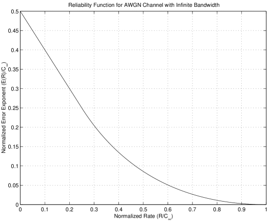
Figure 1: The reliability function for AWGN channel with infinite bandwidth

To establish a strong coding theorem, the reliability function $E(R)$, as defined in [4], of the channel has to be calculated for any coding rate $R$. Generally, the reliability function of a channel is difficult to compute and is known for all rates only for a few channels. Infinite-bandwidth AWGN channel is one of these channels and its reliability function has the following form[15, 4]

$$E(R)=\left\{\begin{array}[]{ll}\frac{C_{\infty}}{2}-R&0\leq R\leq\frac{C_{\infty}}{4};\\ (\sqrt{C_{\infty}}-\sqrt{R})^{2}&\frac{C_{\infty}}{4}\leq R\leq C_{\infty},\\ \end{array}\right.$$ (1)

where $C_{\infty}=P/N_{0}$ denotes the infinite-bandwidth capacity, as shown in Figure 1. We will show that when the bandwidth is infinite, a large set of input distributions can be shown to achieve the optimal error-exponent curve. We will refer to such distributions as being first-order optimal.

Naturally, the results in the infinite bandwidth regime can be considered as guidelines for designing signaling schemes in the wideband regime as well. However, in the wideband regime (when the available bandwidth is large, but finite), the result based on the infinite bandwidth calculations can be quite misleading. In [14], Verdú points out that to understand the performance limit in the wideband regime, two quantities need to be studied: the minimum energy per information bit $({\frac{E_{b}}{N_{0}}}_{min})$ required to sustain reliable communication, and the slope of spectral efficiency (bits/s/Hz) at the point ${\frac{E_{b}}{N_{0}}}_{min}.$ If we treat $C(\cdot)$ as a function of $b=1/B$, it is easy to see that studying these two quantities is equivalent to studying the optimal values of the following two quantities: infinite-bandwidth capacity $C(0)$ and the first-order derivative of capacity with respect to $b$, $\dot{C}(0).$ In other words, we need to study both the infinite-bandwidth capacity, and the rate at which this capacity is reached. In [14], it is shown that, while many signaling schemes achieve $C(0),$ only some of these reach the capacity at the fastest possible rate given by $\dot{C}(0).$ We will refer to signaling schemes that achieve both $C(0)$ and $\dot{C}(0)$ as near-optimal input distributions in the wideband regime. Further, although $C(0)$ always has the same value for non-fading or fading channels with different CSI, $\dot{C}(0)$ is determined by the CSI and can be very different for different channels.

This paper complements Verdú’s work and considers the relationship between probability of decoding error (represented by the reliability function), coding rate, and bandwidth for both AWGN channels and multi-path fading channels. Specifically, we study the maximum rate at which information can be transmitted over a channel, as a function of the available bandwidth, under a certain constraint on the reliability function. For AWGN channels, instead of characterizing the capacity $C$ as a function of $b=1/B$ as in [14], we are interested in characterizing $R_{z}$ as a function of $b,$ where $R_{z}$ is the maximum rate such that $E(R_{z})\geq z$ and $E(R)$ is the reliability function of the channel. In the infinite bandwidth regime, we characterize the optimal rate $R_{z}(0)$ with respect to a certain error-exponent constraint and study the conditions under which a signaling scheme can achieve this optimal rate. In the wideband regime, both $R_{z}(0)$ and $\dot{R_{z}}(0)$ need to be considered. A signaling scheme which can achieve both $R_{z}(0)$ and $\dot{R_{z}}(0)$ is said to be second-order optimal or near optimal with respect to an error-exponent constraint $z.$

For fading channels, we use a doubly-block fading model where the available bandwidth spans multiple coherence bandwidth. If we let $W_{c}$ denote the coherence bandwidth, the total bandwidth of the channel is then assumed to $BW_{c}$ for some $B\geq 1.$ Either a large $B$ or a large $W_{c}$ can lead to a large total bandwidth $BW_{c}.$ However, these two regimes (the large $B$ regime and the large $W_{c}$ regime) can have very different channel behavior. Suppose we consider a wireless system with a total bandwidth of $10$ MHz and if the delay spread is of the order of $1$ $\mu$sec., then $W_{c}$ would be of the order of $1$ MHz and thus, $B$ is of the order of $10.$ In this paper, we focus on such a system where the coherence bandwidth $W_{c}$ is large and further, we assume a coherent channel model. By defining $R_{z}$ to be a function of $1/W_{c},$ we calculate $R_{z}(0)$ and $\dot{R}_{z}(0).$ Similar to the AWGN case, for this channel model, we will show that QPSK can achieve both $R_{z}(0)$ and $\dot{R}_{z}(0)$ and is thus near-optimal. In the other case where $B$ is large, it may not be appropriate to assume any form of channel side information (CSI) and thus a non-coherent channel model is more suitable. We refer the readers to [16] for first-order asymptotic results for MIMO channels in this regime.

This paper is organized as follows. In section 2, we will specify the channel models and formulate the problem that we wish to study. In section 3, we will show the main results for both AWGN channels and multipath fading channels. The proofs will be presented in section 4 and section 5. Section 6 contains concluding remarks and discussions.

2 Channel models and problem formulation

In this section, we will describe the channel models we use to study the behavior of both the AWGN channel and the multipath fading channel in the wideband regime. Further, we will formulate rigorously the problems we want to solve in this paper.

2.1 AWGN channels

We first consider a bandlimited AWGN channel with available bandwidth $B/2:$

$$y(t)=x(t)+w(t),$$ (2)

where $w(t)$ is a complex symmetric Gaussian random process. We assume that we have an input power constraint $P$ for the channel (2). For notational convenience, we assume the noise power density $N_{0}/2=1/2.$ Thus, the average power $P$ also indicates the average SNR of the channel. We now sample the channel at sampling rate $1/B,$ and represent it as a discrete-time memoryless scalar channel as follows:

$$y=x+w,\enskip$$ (3)

where $w$ is a complex symmetric Gaussian random variable with variance $1,$ i.e., $w\in{\mathcal{C}N}(0,1).$ The power constraint for this discrete-time channel is

$$E\left(|x|^{2}\right)\leq\frac{P}{B}.$$ (4)

We want to study the asymptotic behavior of the communication rate $R$ (nats per second) in terms of the available bandwidth $B$ under this power constraint and an error exponent constraint, which is described below.

Let $P_{e}(N,R,P,B)$ be the minimum probability of decoding error for any block code with codeword length $N$ seconds (or equivalently, $NB$ symbols) and coding rate $R.$ The error exponent at communication rate $R$ (also called reliability function) of this channel is defined as

$$E(R,P,B)=\lim_{N\rightarrow\infty}-\frac{\ln P_{e}(N,R,P,B)}{N}.$$ (5)

We desire a lower bound for $E(R,P,B)$ and denote it by $Pz.$ (Without loss of generality, we scale the desired minimum value for the error exponent by $P$ for mathematical convenience.) Let $R_{z}(b)$ denote the maximum possible rate at which communication is possible given this desired error exponent when the available bandwidth is $B=1/b.$ Since $E(P,R,B)$ is a decreasing function of $R,$ $R_{z}(b)$ is the solution to the equation

$$E(P,R,1/b)=Pz.$$ (6)

Our goals for AWGN channels are two-folds:

• Calculate $R_{z}(0)$ and $\dot{R_{z}}(0).$

• Characterize the properties of first-order optimal signaling schemes, i.e., those that achieve $R_{z}(0).$ More importantly, find near-optimal or second-order optimal signaling schemes in the wideband regime such that both $R_{z}(0)$ and $\dot{R}_{z}(0)$ can be achieved.

In the rest of the paper, we drop the subscript and simply refer to $R_{z}$ as $R.$ From the context, it should be clear that $R$ is a function of $z.$

2.2 Coherent fading channels

In this section, we will explain the model we will use for a multi-path fading channel and formulate the problem in the wideband regime we want to solve for such channels.

To characterize a multi-path fading channel, we use a doubly-block Rayleigh fading model. Specifically, we assume block fading in both the time and frequency domains. Further, we assume that we have a rich-scattering environment such that all the fading gains are Gaussian distributed. This model can be visualized as in Figure 2, where we divide the time-frequency plane into blocks of duration $T_{c}$ and bandwidth $W_{c}.$ We assume that the fading is fixed in each block and independent from one block to another. In each block, we can transmit $W_{c}T_{c}$ symbols, from the dimensionality theorem [15]. We let $D=W_{c}T_{c}$ and refer to $D$ as the coherence dimension of the channel.

Figure 2: Doubly-block fading in time-frequency plane

For this channel model, we can represent the channel by

$${\bf y}_{l}=H_{l}{\bf x}_{l}+{\bf w}_{l},\quad 1\leq l\leq B,$$ (7)

where ${\bf x}_{l},{\bf y}_{l},{\bf w}_{l}\in{\mathcal{C}^{D}}.$ In other words, we have $B$ parallel vector channels each with dimension $D.$ Similar to the AWGN channel, we assume there is power constraint $P$ (joule per second) for the fading channel, i.e., we have the following constraint on the input of the channel (7):

$$\sum_{l=1}^{B}E[\|{\bf x}_{l}\|^{2}]\leq PT_{c}.$$ (8)

The doubly-block fading model is a simple approximation of the physical multipath fading channel. However, it retains most of the important characteristics of channels in a fading environment. For a derivation of such a model, we refer the interested reader to [12]. This model has been used in [9] to achieve the lower bound for the optimal bandwidth where spreading still increases non-coherent channel capacity. In [6], Hajek and Subramanian use this model to calculate the reliability function and capacity for a non-coherent fading channel with a small peak constraint on the input signals. However, this model is simpler than the model used by Médard and Gallager [8], which allows correlation in both time and frequency blocks, or the model used Telatar and Tse [11], which allows correlation in frequency blocks.

In the wideband regime, we know the available bandwidth $BW_{c}>>1$ and the energy available per degree of freedom is small, i.e., $\frac{P}{BW_{c}}<<1.$ Obviously, a large bandwidth can be a result of either a large $B$ or a large $W_{c}.$ However, $B$ and $W_{c}$ have different impacts on the channel performance and the asymptotic results in $B$ and $W_{c}$ can be very different from each other and can lead to different conclusions. In this paper, we will focus on the case where $W_{c}$ is large. In this regime, we have large degrees of freedom in each coherence block although the energy per degree of freedom is small. Thus, we might still be able to measure the channel accurately and therefore, we assume a coherent fading channel model in this regime. However, to accurately illustrate the coherence level of this channel model from an error exponent point of view is still a research topic for now. We refer the reader to [17] for a discussion on the relationship between coherence level and coherence length from a capacity point of view.

The ergotic capacity of such channels under full receiver side CSI is well known and is determined by the following expression

$$C=BW_{c}E_{H}[\ln(1+\frac{|H|^{2}P}{BW_{c}})]\quad\textsl{nats per second}.$$ (9)

The reliability function $E(R,P,W_{c})$ of this channel can be defined as below

$$E(R,P,W_{c})=\lim_{N\rightarrow\infty}-\frac{1}{T_{c}}\frac{\ln P_{e}(N,R,P,W_{c})}{N},$$ (10)

where $P_{e}(N,R,P,W_{c})$ is the minimum probability of decoding error for all block codes with codeword length $NT_{c}$ seconds and coding rate $R$ (nats per second).

Let $R_{z}(1/W_{c})$ denote the maximum possible rate at which communication is possible given this desired error exponent $E(R,P,W_{c})\geq z.$ Our goal in studying this channel model in the wideband regime is still two-fold: calculate both $R_{z}(0)$ and $\dot{R}_{z}(0)$ and identify signaling schemes that can achieve $R_{z}(0)$ and $\dot{R}_{z}(0).$

3 Main results

In this section, we will present our main results for AWGN channels and coherent fading channels in two separate sections without proof. Due to the technical nature of the proofs, we will present them in Section 4 and Section 5.

3.1 AWGN channels

We begin by first carefully describing the set of signaling schemes that we will consider in this paper. Due to the technicality in applying the sphere-packing bound (see Appendix A for a short review), we only consider input distributions with a finite alphabet. Specifically, we restrict ourselves to input distributions in the following set.

Definition 1

Define

$${\mathcal{D}}(p)=\{q(x):E[|x|^{2}]=p;\textsl{support of q(x) is a finite set of discrete points in ${\mathcal{C}}$}\}.$$

We impose the following additional constraint on the signaling schemes.

Definition 2

Define ${\mathcal{Q}}(p)$ as a subset of ${\mathcal{D}}(p)$, which satisfies the following properties

$${\mathcal{Q}}(p)=\left\{q_{p}(x)\in{\mathcal{D}}(p):|x|_{max}\leq K_{m}p^{\alpha}.\right\}$$ (11)

where $|{x}|_{max}$ denotes the largest norm among all symbols of the input alphabet. $K_{m}$ and $\alpha$ are allowed to be any positive constants which are independent of $p.$ $\diamond$

In other words, we constrain the input such that the largest-magnitude symbol has to decrease as $B$ increases, although it can decrease at an arbitrarily slow rate. As we will show later, the choice of the parameters $K_{m}$ and $\alpha$ are not relevant to the result. Thus, $K_{m}$ can be an arbitrary large number and $\alpha$ can be an arbitrary small positive number, if we want to make the constraint mild.

A signaling scheme is a sequence of input distributions, parameterized by $B.$ For each $B,$ we can only choose an input distribution from the set ${\mathcal{Q}}(P/B).$

Definition 3

We define ${\mathcal{F}}(P)$ to be the set of signaling schemes, which are parameterized by $B$ and satisfy

$${\mathcal{F}}(P)=\left\{\left\{q_{B}(x)\right\}:q_{B}(x)\in{\mathcal{Q}}(P/B)\right\},$$ (12)

where ${\mathcal{Q}}(P/B)$ is defined by Definition 2. $\diamond$

By choosing signaling schemes from ${\mathcal{F}}(P),$ we are ruling out those peaky signaling schemes in which one of the input symbols remains constant or goes to $\infty,$ while the average power per degree of freeedom goes to $0.$

Under these constraints on the input distribution, we now specify the reliability function $E(R,P,B)$ defined by (5) for AWGN channels.

Lemma 1

Consider the discrete-time additive Gaussian channel (3) with bandwidth $B/2$ and input signaling schemes constrained by ${\mathcal{F}}(P).$ Then the reliability function for this channel satisfies

$$E_{r}(R,P,B)\leq E(R,P,B)\leq E_{sp}(R,P,B),$$ (13)

with

$$E_{r}(R,P,B) =\sup_{0\leq\rho\leq 1}-\rho R+BE_{o}(P/B,\rho),$$

$$E_{sp}(R,P,B) =\sup_{\rho\geq 0}-\rho R+BE_{o}(P/B,\rho),$$

$$E_{o}(P/B,\rho) =\sup_{q\in{\mathcal{Q}}(P/B)}\sup_{\beta\geq 0}-\ln\int\left(\int q(x)e^{\beta\left(|x|^{2}-P/B\right)}f_{w}(y-x)^{\frac{1}{1+\rho}}dx\right)^{1+\rho}dy,$$ (15)

where $f_{w}(x)$ is the probability density function of a complex Gaussian random variable ${\mathcal{C}N}(0,1).$

Proof: This directly follows from the discussion on error exponent in Appendix A. $\diamond$

Remarks: The most important fact here is that as we pointed out in Appendix A, there exists a critical rate $R_{crit},$ such that for $R\geq R_{crit},$ the sphere packing bound and the random-coding bound coincide with each other and thus the random-coding exponent (1) with (15) actually is the true reliability function. Based on this fact, if we only focus on this rate region, by characterizing the asymptotic behavior of (1) when $B$ is large, we get the asymptotic behavior of the reliability function. In the following theorem, we obtain closed-form expressions for $R(0)$ and $\dot{R}(0).$

Theorem 1

Consider the discrete-time additive Gaussian channel (3) with bandwidth $B/2$ and input signaling schemes constrained by ${\mathcal{F}}(P).$ Let $R(1/B)$ be the maximum rate at which information can be transmitted on this channel such that the following error-exponent constraint is satisfied:

$$E(R,P,B)\geq Pz,\quad 0<z<\frac{1}{4}.$$ (16)

We have

$$R(0)=\lim_{B\rightarrow\infty}R(1/B)=P(1-\sqrt{z})^{2},$$ (17)

and

$$\dot{R}(0)=-\frac{P^{2}(1-\sqrt{z})^{3}}{2}.$$ (18)

$\diamond$

Remarks: The constraint on $z$ in (16) arises from the fact that the reliability function is only determined for a certain range of $z.$ Outside this range, the random-coding exponent is not necessarily tight. As we will show later, $z=\frac{1}{4}$ is the error exponent for $R=R_{crit}$ in the infinite bandwidth limit. We now argue that for $0<z<\frac{1}{4},$ when the bandwidth is sufficiently large, the solution $R(1/B)$ to (16) will exceed $R_{crit}(1/B)$ and thus, the error exponent at $R(1/B)$ is equal to the random-coding exponent. To be precise, we state this argument in the following lemma and provide the proof in the appendix. It follows from this lemma that we can represent the reliability function by the random-coding exponent if we only consider $z<\frac{1}{4}.$

Lemma 2

Let $R_{r}(1/B)$ be the solution to the random-coding exponent constraint $E_{r}(R,P,B)=Pz,$ for a fixed $z\in(0,\frac{1}{4}).$ For a fixed $z<\frac{1}{4},$ we must be able to find a $B_{z}<\infty,$ such that for all $B>B_{z},$ $R(1/B)=R_{r}(1/B).$

Proof: See Appendix B. $\diamond$

It should be noted that the constraints on the input signaling are not necessary to obtain the first-order result (17). In other words, introducing peakiness or allowing continuous alphabet symbols in the input distributions will not improve the error exponent in the infinite bandwidth limit for the AWGN channel. These constraints only play a role in obtaining the second-order terms in the expansion of $R_{z}(1/B)$ around $1/B=0.$

A main goal of our study of the wideband reliability function here is to find good signaling schemes in the sense that they can achieve $R(0)$ and $\dot{R}(0).$ To do that, we first define first-order optimality and near optimality (or second-order optimality) formally of a signaling scheme in the wideband regime, in a similar way as in [14].

Definition 4

Consider a signaling scheme $\{q_{B}({\bf x})\}\in{\mathcal{F}}(P)$ parameterized by $B.$ Let $\tilde{R}(1/B)$ be the solution of

$$Pz=E(R,q_{B},P,B)$$ (19)

where $E(R,q_{B},P,B)$ is the reliability function of the channel when the input distribution is fixed to be $q_{B}.$ This signaling scheme is said to be first-order optimal with respect to the normalized error exponent $z$, if

$${\tilde{R}}(0)={R}(0).$$

$\diamond$

Definition 5

A signaling scheme $\{q_{B}({\bf x})\}\in{\mathcal{F}}(P)$ is called second-order optimal or near optimal with respect to the normalized error exponent $z$ if

$${\tilde{R}}(0)=R(0);$$ (20)

$$\dot{\tilde{R}}(0)=\dot{R}(0),$$ (21)

where $\tilde{R}(1/B)$ is the solution to (19). $\diamond$

For AWGN channels, we obtain a sufficient condition for a signaling scheme to be first-order optimal. Then, we study the performance of two simple signaling schemes as in [14]: BPSK and QPSK. Specifically, when we say BPSK or QPSK, we mean the following. Let $p=P/B$ be the available power per degree of freedom. For BPSK, we choose the input to be either $\sqrt{p}$ or $-\sqrt{p}$ with equal probability; for QPSK, the input alphabet consists of $\sqrt{\frac{p}{2}}(1+j)$, $\sqrt{\frac{p}{2}}(1-j)$, $\sqrt{\frac{p}{2}}(-1+j)$, and $\sqrt{\frac{p}{2}}(-1-j)$, all chosen with equal probability as well.

Theorem 2

For AWGN channels, all signaling schemes in ${\mathcal{F}}(P)$ which are symmetric around $0$ are first-order optimal for any given $z\in(0,\frac{1}{4})$. Thus, both BPSK and QPSK are first-order optimal; however, only QPSK is second-order optimal. $\diamond$

Remarks: From this theorem, we know that it does not take much for a signaling scheme to be first-order optimal. This result is consistent with the capacity result shown by Massey in [7].

To get a better feel for how differently BPSK and QPSK behave in the wideband regime, we plot $R$ as a function of $1/B$ for both BPSK and QPSK in Figure 3. As shown in Figure 3, as $B\rightarrow\infty,$ both BPSK and QPSK can achieve the optimal rate $R(0).$ However, only QPSK can achieve $\dot{R}(0).$

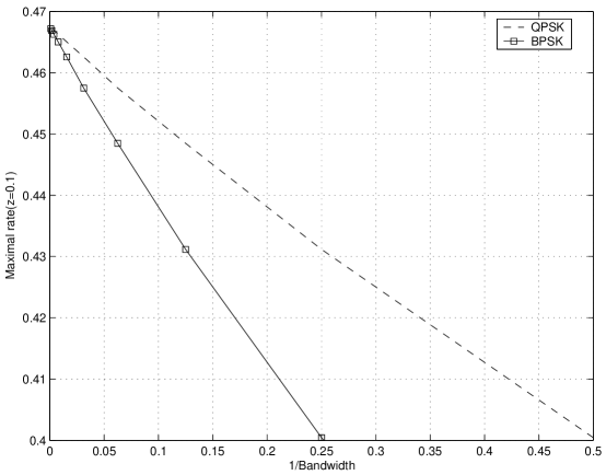
Figure 3: The maximal rate $R$ for BPSK and QPSK for a fixed normalized error exponent $z=0.1.$

Another way to understand the difference between the performance of BPSK and QPSK is to study the fundamental tradeoff between spectral efficiency and energy per information bit ($E_{b}/N_{0}$), as suggested in [14]. We plot this tradeoff in Figure 4. From this figure, we can see that both BPSK and QPSK can achieve the optimal ${\frac{E_{b}}{N_{0}}}_{min},$ however, only QPSK can achieve the optimal spectral efficiency slope at the point ${\frac{E_{b}}{N_{0}}}_{min}.$

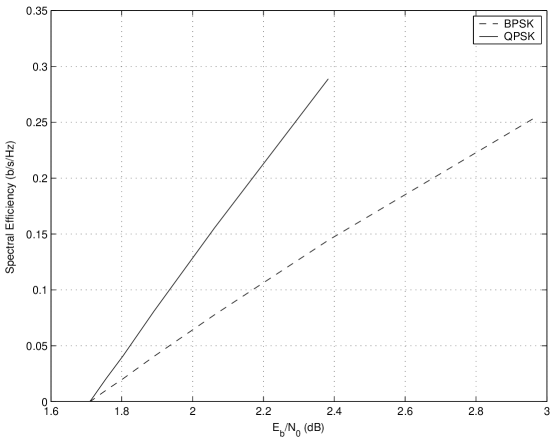
Figure 4: Spectral efficiencies achieved by QPSK and BPSK in the AWGN channel, when the error exponent is constrained by $z=0.1.$

As compared to Figure 2 in [14], the major difference here is that ${\frac{E_{b}}{N_{0}}}_{min}$ in Figure 4 is around $3.3dB$ higher, since we have a more stringent constraint than just reliable communications, as considered in [14]. ${\frac{E_{b}}{N_{0}}}_{min}$ here denotes the minimal energy per information bit such that the probability of error has to decay faster than $e^{-Nz}$ as the codeword length $N$ increases.

3.2 Coherent fading channels

Next, we consider coherent fading channels. As in the case of the AWGN channel, we first describe our assumptions on the input signaling schemes.

Definition 6

Define $\mathcal{Q}^{B}_{W_{c}}(P)$ to be the set of joint input distributions on ${\bf X}=({\bf x}_{1},{\bf x}_{2},\cdots,{\bf x}_{B}),$ where $\{{\bf x}_{l},\enskip l=1,2,\cdots,B\}$ are vectors with dimension $D=W_{c}T_{c},$ which satisfy the following

• the average power constraint (8) is satisfied;

• the distribution has a discrete alphabet, consisting of finite number of symbols;

• each symbol can be chosen from a given set ${\mathcal{S}}^{B}_{W_{c}}.$ The set of symbols ${\mathcal{S}}^{B}_{W_{c}}$ is defined as follows:

  $${\mathcal{S}}^{B}_{W_{c}}=\{{\bf X}=\{{\bf x}_{1},{\bf x}_{2},\cdots,{\bf x}_{B}\}:{\bf x}_{l}\in C^{D};\max_{d=1,2,\cdots D}|x_{ld}|\leq K_{m}W_{c}^{-\alpha}\enskip\forall l=1,2,\cdots,B\},$$ (22)

  where $K_{m}$ and $\alpha$ are allowed to be any positive constants independent of $W_{c}.$ $\diamond$

The signaling schemes of interest to us are defined as follows.

Definition 7

We define ${\mathcal{F}}^{B}_{W_{c}}(P)$ to be the set of signaling schemes, which are parameterized by $W_{c}$ and satisfy

$${\mathcal{F}}^{B}_{W_{c}}(P)=\left\{\left\{q_{W_{c}}({\bf X})\right\}:q_{W_{c}}({\bf X})\in{\mathcal{Q}}^{B}_{W_{c}}(P)\right\},$$ (23)

where ${\mathcal{Q}}^{B}_{W_{c}}(P)$ was defined in Definition 6. $\diamond$

The reliability function for our discrete-time channel model (7) with signaling schemes constrained by ${\mathcal{F}}_{W_{c}}^{B}(P)$ can be computed according to the following lemma.

Lemma 3

Consider the coherent fading channel model (7) with $H$ known at the receiver. Assume that the input distribution satisfies the average power constraint (4) and the constraint in in ${\mathcal{F}}_{W_{c}}^{B}(P).$ The reliability function $E(R,P,W_{c})$ satisfies

$$E_{r}(R,P,W_{c})\leq E(R,P,W_{c})\leq E_{sp}(R,P,W_{c}),$$

with

$$E_{r}(R,P,W_{c}) = \sup_{0\leq\rho\leq 1}-\rho R+E_{o}(P,\rho,W_{c}),$$

$$E_{sp}(R,P,W_{c}) = \sup_{\rho\geq 0}-\rho R+E_{o}(P,\rho,D),$$

$$E_{o}(P,\rho,W_{c}) = \sup_{q\in{\mathcal{F}}_{W_{c}}^{B}(P)}\sup_{\beta\geq 0}-\frac{1}{T_{c}}\ln E_{H}\int\left(\int q({\bf X})e^{\beta(\|{\bf X}\|^{2}-PT_{c})}f({\bf Y}|{\bf X},{\bf H})^{\frac{1}{1+\rho}}d{\bf X}\right)^{1+\rho}d{\bf Y}.$$ (24)

Proof: We can apply Theorem 15 and Theorem 16 from Appendix A here to this channel model by viewing the channel as a memoryless channel with output $\hat{\bf Y}=\{{\bf Y},{\bf H}\}.$ The fraction of $\frac{1}{T_{c}}$ in (24) is to balance the scaling since the rate $R$ here is defined to be nats per second. $\diamond$

The constraint on the error exponent is

$$E(R,P,W_{c})\geq z,$$ (25)

and we need to solve for $R(0)$ and $\dot{R}(0)$ where $R$ is a function for $\frac{1}{W_{c}}$ for a fixed $B.$ We have the following theorem.

Theorem 3

Consider a coherent Rayleigh-fading vector channel (7) with the input signaling constrained by ${\mathcal{F}}^{B}_{W_{c}}(P).$ Let $R(1/W_{c})$ be the maximum rate at which information can be transmitted on this channel such that the following error-exponent constraint is satisfied:

$$E(R,P,W_{c})\geq z,\quad 0<z<z^{*},$$ (26)

where $z^{*}$ is defined as follows

$$z^{*}=\frac{B}{T_{c}}\ln(1+\frac{PT_{c}}{2B})-\frac{P}{4+2PT_{c}/B}.$$ (27)

We have

$$R(0)=\lim_{W_{c}\rightarrow\infty}R_{B}(1/W_{c})=\sup_{0\leq\rho\leq 1}-\frac{z}{\rho}+\frac{1}{T_{c}}\frac{B\ln\left(1+\frac{\rho PT_{c}}{B(1+\rho)}\right)}{\rho},$$ (28)

and

$$\dot{R}(0)=-\frac{P^{2}}{B(1+\rho)(1+\rho^{*}+\frac{\rho^{*}PT_{c}}{B})^{2}},$$ (29)

where $\rho^{*}$ is the optimizing $\rho$ in (28). $\diamond$

The constraint on $z$ in (26) again comes from the fact that the reliability function is only known when $R\geq R_{crit}.$ Now we show that $z^{*}$ given by (27) is the corresponding error exponent at $R_{crit}$ when $W_{c}$ goes to infinity. From the property of the critical rate $R_{crit},$ we know the optimizing $\rho$ in (28) at the corresponding error exponent $z_{crit}$ is $1.$ Thus, taking derivative of the right side of (28) with respect to $\rho,$ we must have

$$\frac{z_{crit}}{\rho^{2}}-\frac{B}{T_{c}}\frac{\ln(1+\frac{\rho PT_{c}}{B(1+\rho)})}{\rho^{2}}+\frac{B}{T_{c}}\frac{PT_{c}/B}{\rho(1+\frac{\rho PT_{c}}{B(1+\rho)})}\frac{1}{(1+\rho)^{2}}|_{\rho=1}=0.$$

By solving this, it is straightforward to have $z_{crit}=z^{*}$ with $z^{*}$ determined by (27). The corresponding rate $R_{crit}$ can be obtained as follows

$$R_{crit} = -z_{crit}+\frac{B}{T_{c}}\ln(1+\frac{PT_{c}}{2B})$$

$$= \frac{P}{4+2\frac{PT_{c}}{B}}.$$

Using a similar argument as in the AWGN channel case, we can argue that for $z\in(0,z^{*}),$ the reliability function coincides with the random-coding exponent for sufficiently large $W_{c}$ . Thus, the calculation of $R(0)$ and $\dot{R}(0)$ can be carried out by using the random-coding exponent.

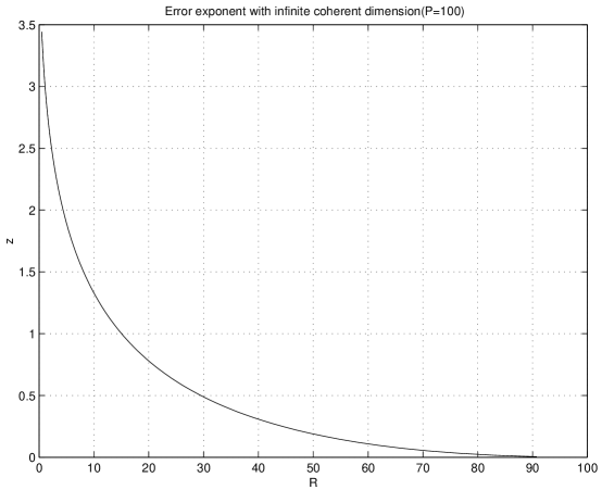
Figure 5: The error exponent curve from $R_{crit}$ to capacity for the channel with infinite coherence dimension. $B=T_{c}=1.$ $P=100.$

Another observation here is that the applicable region (in terms of $R$), where the random-coding exponent coincides with the sphere-packing exponent, actually covers most of the rate region from $0$ to capacity, when the available energy per coherence block $\frac{PT_{c}}{B}$ is fairly large. To see this, we first notice that as $W_{c}$ goes to infinity, our capacity $C_{\infty}$ in (9) is $P.$ Thus, the critical rate $R_{crit}$ can be also written as $\frac{1}{4+2\frac{PT_{c}}{B}}C_{\infty}.$ When $\frac{PT_{c}}{B}$ is large, we have $R_{crit}<<C_{\infty}.$ This observation is also shown in Figure 5. For simplicity, we choose $B=T_{c}=1$ in this numerical example and choose $P=100.$

Next, we need to identify those signaling schemes which can achieve $R(0)$ and $\dot{R}(0).$ Again, we consider BPSK and QPSK signaling. However, for the fading channel (7), these two signaling schemes have slightly different meanings than what we defined in last section for AWGN channels. Specifically, for both BPSK and QPSK, we spread the available power in each coherent block equally among all the time-frequency coherent blocks and make the distributions in each dimension i.i.d. For BPSK, the symbols for each dimension are $\sqrt{P/BW_{c}}$ and $-\sqrt{P/BW_{c}},$ with equal probability. For QPSK, the symbols are $\sqrt{\frac{P}{2BW_{c}}}(1+j)$, $\sqrt{\frac{P}{2BW_{c}}}(1-j)$, $\sqrt{\frac{P}{2BW_{c}}}(-1+j)$ and $\sqrt{\frac{P}{2BW_{c}}}(-1-j).$ Similar to the AWGN case, we have

Theorem 4

Both BPSK and QPSK are first-order optimal for any given $z\in(0,z^{*})$; however, only QPSK is second-order optimal. $\diamond$

3.3 Implications and discussion

The results that we have obtained for both AWGN channels and coherent fading channels are consistent with the results from a capacity point of view in the seminal work [14]. By letting $z$ go to $0,$ the quantity $R_{z}$ becomes the capacity of the channel. Thus, it can be easily checked that by taking $z$ to be $0,$ we can recover the capacity results by using the expressions in Theorem 1 and Theorem 3. However, we also have to point out that in [14], a very general treatment is provided for a much broader class of channel models. In this paper, due to the complexity of the calculation of the reliability function, we only calculated the first and second order rate approximation for two very specific channel models.

Despite the similarity between our results and Verdu’s results regarding near-optimal signaling, the fact that QPSK is still near-optimal under a certain error exponent constraint is still somewhat surprising because of the following reason. In general, very little is known about the conditions under which an input distribution achieves the optimal error exponent at a given rate, even in the infinite bandwidth limit. It is not necessarily true that capacity-achieving distributions are also optimal from an error-exponent point of view. One example is the infinite-bandwidth non-coherent Rayleigh fading channel, which is studied in [16]. Thus, it is not obvious that actually QPSK can do well in the wideband regime from an error exponent point of view,even though it is wideband optimal from a capacity point of view.

4 Proof of Theorem 1 and Theorem 2

Due to the technical nature of the calculations needed in the proofs of our main results, we first summarize the proof steps as follows to help the reader follow the proof of our main results.

The proof of Theorem 1 can be broken down into the following major steps:

• We first relate the problem of finding $R(0)$ and $\dot{R}(0),$ where $R$ is the communication rate per second as a function of $1/B,$ to the problem of finding $\dot{r}(0)$ and $\ddot{r}(0),$ where $r$ is the communication rate per degree of freedom in (3) as a function of $p,$ which denotes the SNR per degree of freedom.

• The calculation of $\dot{r}(0)$ can be related to the optimal value for $E_{o}$ in the infinite bandwidth limit; an upper bound is derived for $E_{o}$ using a simple inequality; this bound is further shown to be achievable;

• $\ddot{r}(0)$ can also be related to certain derivatives of $E_{o}$; a better upper bound is derived for $E_{o}$ which yields an upper bound for $\ddot{r}(0);$ this bound is also shown to be achievable.

The next several subsections will prove the main results following these three steps.

4.1 Communication rate and error exponent per degree of freedom

It is shown in [14] that the capacity $C$ in a bandlimited channel with limited available power $P,$ but large available bandwidth $B,$ can be related to the capacity $c$ in a scalar channel with small available power $p=P/B.$ Thus, the problem of finding optimal $C(0)$ and $\dot{C}(0)$ can be shown to be equivalent to the problem of finding optimal $\dot{c}(0)$ and $\ddot{c}(0)$. The relationship between $C(0)$ and $\dot{c}(0)$ is also extensively studied in an earlier paper [13], where the notion capacity per unit cost was studied. We first show that a similar connection can be made between the error-exponent constrained rates $R$ (nats per second) and $r$ (nats per symbol).

Theorem 5

Consider a scalar Gaussian channel $y=x+w$ with average power constraint $p.$ Further, the signaling schemes are constrained by ${\tilde{\mathcal{F}}}(p)=\left\{\left\{q_{p}({x})\right\}:q_{p}({x})\in{\mathcal{Q}}(p)\right\}.$ Let $r$ be the maximum rate per symbol at which information can be transmitted through channel (3) such that the error exponent satisfies

$$\hat{E}(r,p)\geq pz,\quad 0<z<\frac{1}{4},$$

where $\hat{E}(r,p)$ is the error exponent per symbol of the scalar channel with power constraint $p.$ Consider $r$ as a function of $p.$ Let $R$ (nats per second) be defined as the solution to (16). We have

$$R(0) = P\dot{r}(0);$$

$$\dot{R}(0) = \frac{P^{2}\ddot{r}(0)}{2}.$$

Proof: It is easy to check that

$$E(R,P,B)=B\hat{E}(R/B,P/B).$$

Denoting $r=R/B$ and $p=P/B,$ the original error-exponent constraint can be rewritten as

$$\hat{E}_{r}(r,p)\geq pz.$$

Using these two relations and considering $R$ as a function of $b=1/B,$ we have

$$R(0) = \lim_{b\rightarrow 0}R(b)=\lim_{b\rightarrow 0}\frac{r(p)}{b}=P\lim_{b\rightarrow 0}\frac{r(p)}{p}=P\dot{r}(0)$$ (30)

$$\dot{R}(0) = \lim_{b\rightarrow 0}\frac{R(b)-R(0)}{b}=\lim_{b\rightarrow 0}\frac{\frac{1}{b}r(Pb)-R(0)}{b}=\frac{P^{2}\ddot{r}(0)}{2}$$ (31)

$\diamond$

Thus, the original problem of finding $R(0)$ and $\dot{R}(0)$ in the wideband regime is equivalent to finding the optimal values for $\dot{r}(0)$ and $\ddot{r}(0),$ given a constraint on the reliability function $\hat{E}(r,p)\geq pz.$ In the rest of this paper, we will deal with this scalar channel problem. For notational convenience, we use $E(r,p)$ to denote the error exponent per symbol of the single channel instead of using ${\hat{E}}(r,p).$

4.2 Optimal value of $\dot{r}(0)$

We know for the error-exponent constraint in the range of $(0,\frac{1}{4})$ and $p$ sufficiently small, we have

$$E(r,p)=E_{r}(r,p)=\sup_{0\leq\rho\leq 1}-\rho r+E_{o}(p,\rho),$$

where

$$E_{o}(p,\rho)=\sup_{q_{p}\in{\tilde{\mathcal{F}}}(p)}\sup_{\beta\geq 0}-\ln\int\left(\int q_{p}(x)e^{\beta(|x|^{2}-p)}f(y|x)^{\frac{1}{1+\rho}}dx\right)^{1+\rho}dy.$$ (32)

Thus, the constraint on the error exponent can also be written as

$$pz=\sup_{0\leq\rho\leq 1}-\rho r+E_{o}(p,\rho).$$ (33)

The first result in the first-order calculation is the following lemma.

Lemma 4

For any $\rho\in[0,1],$ $E_{o}(p,\rho)$ is upper bounded by

$$E_{o}(p,\rho)\leq\frac{p\rho}{1+\rho}.$$ (34)

Proof: For notational convenience, define $\alpha(y)$ to be

$$\alpha(y)=\int q_{p}(x)e^{\beta(|x|^{2}-p)}f(y|x)^{\frac{1}{1+\rho}}dx$$ (35)

and $M(y)$ as

$$M(y)=\int q_{p}(x)e^{\beta(|x|^{2}-p)}\left[\frac{f(y|x)}{f(y|0)}\right]^{\frac{1}{1+\rho}}dx.$$ (36)

Here $f(y|0)$ denotes the distribution function of $y$ conditioned on that the input is $0.$ It is easy to see that $f(y|0)$ is simply the distribution of the Gaussian noise $f_{w}(y).$ Then we have

$$E_{o}(p,\rho) = \sup_{q\in{\tilde{\mathcal{F}}}(p)}\sup_{\beta\geq 0}-\ln\int\alpha(y)^{1+\rho}dy$$ (37)

$$= \sup_{q\in{\tilde{\mathcal{F}}}(p)}\sup_{\beta\geq 0}-\ln\int f_{w}(y)M(y)^{1+\rho}dy$$

$$\leq \sup_{q\in{\tilde{\mathcal{F}}}(p)}\sup_{\beta\geq 0}-\ln\left(\int f_{w}(y)M(y)dy\right)^{1+\rho}$$ (38)

$$= \sup_{q\in{\tilde{\mathcal{F}}}(p)}\sup_{\beta\geq 0}-(1+\rho)\ln E_{q}\left[e^{\beta(|x|^{2}-p)}\int f_{w}(y)^{\frac{\rho}{1+\rho}}f(y|x)^{\frac{1}{1+\rho}}dy\right]$$ (39)

$$= \sup_{q\in{\tilde{\mathcal{F}}}(p)}\sup_{\beta\geq 0}-(1+\rho)\ln E_{q}\left[e^{\beta(|x|^{2}-p)}\int f_{w}(y)^{\frac{\rho}{1+\rho}}f_{w}(y-x)^{\frac{1}{1+\rho}}dy\right]$$ (40)

$$= \sup_{q\in{\tilde{\mathcal{F}}}(p)}\sup_{\beta\geq 0}-(1+\rho)\ln E_{q}\left[e^{\beta(|x|^{2}-p)}e^{-\theta|x|^{2}}\right]$$ (41)

$$\leq \sup_{q\in{\tilde{\mathcal{F}}}(p)}\sup_{\beta\geq 0}-(1+\rho)\ln e^{-\theta p}$$

$$= \frac{\rho p}{1+\rho},$$

where $\theta$ in (41) is defined by

$$\theta=\frac{\rho}{(1+\rho)^{2}}.$$

The inequalities in (38) and (4.2) are simple applications of Jensen’s inequality. $\diamond$

The next theorem establishes an alternate expression for the error exponent constraint (33).

Theorem 6

The error-exponent constraint (33) implies the following relationship between $r$ and $z$

$$r=\sup_{0\leq\rho\leq 1}-\frac{pz}{\rho}+\frac{E_{o}(p,\rho)}{\rho}.$$ (43)

Proof: See Appendix C. $\diamond$

Since we want to study the first and second-order derivative of $r$ with respect to $p$ in the low SNR regime, it is more convenient to use (43). To obtain the first order derivative, from (43) we first note that

$$\frac{r}{p}=\sup_{0\leq\rho\leq 1}-\frac{z}{\rho}+\frac{E_{o}(p,\rho)}{p\rho}.$$

Now we relate $\dot{r}(0)$ to the first partial derivative of $E_{o}(p,\rho)$ with respect to $p.$

Theorem 7

If as $p\rightarrow 0,$ the limit of $\frac{E_{o}(p,\rho)}{p}$ exists for any $\rho\in[0,1],$ which is denoted as $\dot{E}_{o}(0,\rho),$ and further,

$$\frac{E_{o}(p,\rho)}{p\rho}\rightarrow\frac{\dot{E_{o}}(0,\rho)}{\rho}\quad\textsl{uniformly for $\rho\in[0,1],$}$$

we have

$$\dot{r}(0)=\sup_{0\leq\rho\leq 1}-\frac{z}{\rho}+\frac{\dot{E}_{o}(0,\rho)}{\rho}.$$ (44)

Proof: From the definition of uniform convergence, for any $\epsilon>0,$ we can find $\delta(\epsilon)>0,$ such that for any $p<\delta(\epsilon),$ we have

$$\left|\frac{E_{o}(p,\rho)}{p\rho}-\frac{\dot{E_{o}}(0,\rho)}{\rho}\right|<\epsilon,\quad\forall\rho\in[0,1].$$

Thus, if we denote $K=\sup_{0\leq\rho\leq 1}-\frac{z}{\rho}+\frac{\dot{E}_{o}(0,\rho)}{\rho},$ we have

$$\frac{r(p)}{p}\leq\sup_{0\leq\rho\leq 1}-\frac{z}{\rho}+\frac{\dot{E_{o}}(0,\rho)}{\rho}+\epsilon=K+\epsilon.$$

Similarly, we can show that $\frac{r(p)}{p}\geq K-\epsilon.$ Letting $\epsilon\rightarrow 0,$ we have $\dot{r}(0)=\lim_{p\rightarrow 0}\frac{r(p)}{p}=K.$ $\diamond$

Lemma 5

As $p\rightarrow 0,$ $\frac{E_{o}(p,\rho)}{p\rho}$ converges to $\frac{1}{1+\rho}$ uniformly for $\rho\in[0,1].$

Proof: In Lemma 4, we have already shown that

$$\frac{E_{o}(p,\rho)}{p\rho}\leq\frac{1}{1+\rho}.$$

In Appendix I, we will show that when the input distribution is chosen to be BPSK or QPSK, $\frac{{\tilde{E}}_{o}(p,q_{p},\rho)}{p\rho}$ converges uniformly to $\frac{1}{1+\rho}.$ Since $\frac{E_{o}(p,\rho)}{p\rho}$ is lower bounded by $\frac{{\tilde{E}}_{o}(p,q_{p},\rho)}{p\rho},$ the lemma follows. $\diamond$

Using Lemma 5 and Theorem 7, we can compute $\dot{r}(0).$

Proposition 1

For $0<z<\frac{1}{4},$

$$\dot{r}(0)=(1-\sqrt{z})^{2}.$$ (45)

Proof: From Theorem 7, we have

$$\dot{r}(0) = \sup_{0\leq\rho\leq 1}-\frac{z}{\rho}+\frac{\dot{E}_{o}(0,\rho)}{\rho}$$

$$= \sup_{0\leq\rho\leq 1}-\frac{z}{\rho}+\frac{1}{1+\rho}$$

$$= \left\{\begin{array}[]{ll}(1-\sqrt{z})^{2}&0\leq z\leq\frac{1}{4};\\ \frac{1}{2}-z&\frac{1}{4}\leq z\leq 1.\\ \end{array}\right.$$ (49)

For $0<z<\frac{1}{4},$ the optimizing $\rho^{*}=\frac{\sqrt{z}}{1-\sqrt{z}}.$ $\diamond$

Note here the optimal value $\dot{r}(0)$ is obtained by optimizing over all input distributions in ${\tilde{\mathcal{F}}}(p).$ However, this result is valid for all input distributions. In other words, allowing continuous alphabet or peaky signaling would not change this optimal value. This is due to the well-known infinite bandwidth AWGN channel error-exponent result, which is shown in (1). It can be easily seen that (45) is simply the inverse function of (1). The purpose of deriving $\dot{r}(0)$ using the constraint ${\tilde{\mathcal{F}}}(p)$ is not to just derive (45), but also to obtain conditions on the input distributions in ${\tilde{\mathcal{F}}}(p)$ which achieve (45). We will obtain such conditions in the next subsection.

4.3 First-order optimality condition

Next we study conditions for a sequence of input distributions to be first-order optimal.

Lemma 6

Assuming $0<z<\frac{1}{4}$, a sufficient condition for $\{q_{p}\}\in{\tilde{\mathcal{F}}}(p)$ to be first-order optimal is that

$$\lim_{p\rightarrow 0}\frac{{\tilde{E}}_{o}(p,q_{p},\rho^{*})}{p}=\frac{\rho^{*}}{1+\rho^{*}},$$ (50)

where $\rho^{*}=\frac{\sqrt{z}}{1-\sqrt{z}}$.

Proof: If $\lim_{p\rightarrow 0}\frac{{\tilde{E}}_{o}(p,q_{p},\rho^{*})}{p}=\frac{\rho^{*}}{1+\rho^{*}},$ we have

$$\liminf_{p\rightarrow 0}\frac{\tilde{r}}{p} \geq \liminf_{p\rightarrow 0}-\frac{z}{\rho^{*}}+\frac{{\tilde{E}}_{o}(p,q_{p},\rho^{*})}{p\rho^{*}}$$

$$= -\frac{z}{\rho^{*}}+\lim_{p\rightarrow 0}\frac{{\tilde{E}}_{o}(p,q_{p},\rho^{*})}{p\rho^{*}}$$

$$= -\frac{z}{\rho^{*}}+\frac{1}{1+\rho^{*}}$$

$$= (1-\sqrt{z})^{2}.$$

On the other hand, from Lemma 4, we know

$$\limsup_{p\rightarrow 0}\frac{\tilde{r}}{p} = \limsup_{p\rightarrow 0}\sup_{0\leq\rho\leq 1}-\frac{z}{\rho}+\frac{{\tilde{E}}_{o}(p,q_{p},\rho)}{p\rho}$$

$$\leq \limsup_{p\rightarrow 0}\sup_{0\leq\rho\leq 1}-\frac{z}{\rho}+\frac{E_{o}(p,\rho)}{p\rho}$$

$$\leq \limsup_{p\rightarrow 0}\sup_{0\leq\rho\leq 1}-\frac{z}{\rho}+\frac{1}{1+\rho}$$

$$= (1-\sqrt{z})^{2}.$$

Thus, the limit of $\frac{\tilde{r}}{p}$ exists and we have

$$\dot{\tilde{r}}(0)=\lim_{p\rightarrow 0}\frac{\tilde{r}}{p}=(1-\sqrt{z})^{2}.$$

$\diamond$

Actually, it does not take much to be first-order optimal.

Lemma 7

For a fixed $0<z<\frac{1}{4},$ a sequence of input distribution ${q_{p}}\in{\tilde{\mathcal{F}}}(p)$ is first-order optimal if it is symmetric around $0.$

Proof: Refer to Appendix H. $\diamond$

4.4 The optimal value of $\ddot{r}(0)$

In this section, we will find an upper bound for $\ddot{r}(0)$ and later we will show that this value is achievable. To do this, we first connect $\ddot{r}(0)$ to the second partial derivative of $E_{o}(p,\rho)$ with respect to $p.$

Theorem 8

Assume the second partial derivative of $E_{o}(p,\rho)$ with respect to $p$ at $p=0$ (denoted as $\ddot{E}_{o}(0,\rho)$) exists for any $\rho\in[0,1].$ Further, assume that

$$\frac{\frac{E_{o}(p,\rho)}{p\rho}-\frac{\dot{E}_{o}(0,\rho)}{\rho}}{p}\rightarrow\frac{\ddot{E}_{o}(0,\rho)}{2\rho}\quad\textsl{uniformly for $\rho\in[0,1]$},$$

and $\frac{\ddot{E}_{o}(0,\rho)}{\rho}$ is a continuous and bounded function of $\rho$ for $\rho\in[0,1].$ Then $\ddot{r}(0)$ can be determined by

$$\ddot{r}(0)=\frac{\ddot{E}_{o}(0,\rho^{*})}{\rho^{*}},$$ (51)

where $\rho^{*}$ is the optimal $\rho$ in (44) and is equal to $\frac{\sqrt{z}}{1-\sqrt{z}}.$

Proof: First we show that

$$\ddot{\overline{r}}(0)=\limsup_{p\rightarrow 0}\frac{r(p)-p\dot{r}(0)}{p^{2}/2}\leq\frac{\ddot{{E}}_{o}(0,\rho^{*})}{\rho^{*}}.$$

The uniform convergence gives us: for any $\epsilon>0,$ we can find $\eta(\epsilon)$ such that for all $p<\eta(\epsilon),$

$$\left|\frac{\frac{E_{o}(p,\rho)}{p\rho}-\frac{\dot{E}_{o}(0,\rho)}{\rho}}{p}-\frac{\ddot{E}_{o}(0,\rho)}{2\rho}\right|<\epsilon\quad\textsl{for all $\rho\in[0,1]$}.$$

In other words, for $p<\eta(\epsilon),$ we can write

$$E_{o}(p,\rho)\leq\dot{{E}}_{o}(0,\rho)p+\ddot{E}_{o}(0,\rho)p^{2}/2+\rho\epsilon p^{2}.$$

From (43), we have

$$r(p)\leq\sup_{0\leq\rho\leq 1}-\frac{pz}{\rho}+\frac{\dot{{E}}_{o}(0,\rho)p+\ddot{E}_{o}(0,\rho)p^{2}/2}{\rho}+\epsilon p^{2}.$$ (52)

Assume $\rho(p)$ is the optimizing $\rho$ for (52). From the first-order calculation, we already know that

$$\dot{E}_{o}(0,\rho)=\frac{\rho}{1+\rho}.$$

Since the optimization in (52) is performed over a compact set $[0,1]$ and by assumption $\ddot{E}_{o}(0,\rho)$ is continuous in $\rho,$ the optimizing $\rho$ must exist.

We must have

$$r(p) \leq \left\{\sup_{0\leq\rho\leq 1}-\frac{pz}{\rho}+\frac{p\dot{{E}}_{o}(0,\rho)}{\rho}\right\}+\frac{\ddot{{E}}_{o}(0,\rho(p))\frac{p^{2}}{2}}{\rho(p)}+\epsilon p^{2}.$$

From (44), we know

$$\dot{r}(0)p=\sup_{0\leq\rho\leq 1}-\frac{pz}{\rho}+\frac{p\dot{{E}}_{o}(0,\rho)}{\rho}.$$

This gives us

$$\frac{r(p)-p\dot{r}(0)}{p^{2}/2}\leq\frac{\ddot{{E}}_{o}(0,\rho(p))}{\rho(p)}+2\epsilon.$$

Letting $\epsilon$ go to $0$, we have

$$\ddot{\overline{r}}(0) = \limsup_{p\rightarrow 0}\frac{r(p)-p\dot{r}(0)}{p^{2}/2}$$ (53)

$$\leq \limsup_{p\rightarrow 0}\frac{\ddot{{E}}_{o}(0,\rho(p))}{\rho(p)}$$

$$= \frac{\ddot{{E}}_{o}(0,\rho^{*})}{\rho^{*}},$$

where $\rho^{*}$ is the optimizing $\rho$ of (52) as $p$ goes to zero, and can be shown to be equal to $\frac{\sqrt{z}}{1-\sqrt{z}}.$ The last equation (53) can be easily verified given that $\frac{\ddot{E}_{o}(0,\rho)}{\rho}$ is a continuous function of $\rho,$ if we have $\lim_{p\rightarrow 0}\rho(p)=\rho^{*},$ which we will show in Appendix D.

To complete the proof of the theorem, it suffices to show

$$\ddot{\underline{r}}(0)=\liminf_{p\rightarrow 0}\frac{r(p)-p\dot{r}(0)}{p^{2}/2}\geq\frac{\ddot{{E}}_{o}(0,\rho^{*})}{\rho^{*}}.$$

To see this, we choose $\rho=\rho^{*}$ in (52) and we have

$$r(p) \geq -\frac{pz}{\rho^{*}}+\frac{p\dot{{E}}_{o}(0,\rho^{*})}{\rho^{*}}+\frac{\ddot{{E}}_{o}(0,\rho^{*})\frac{p^{2}}{2}}{\rho^{*}}-\epsilon p^{2}.$$

From (44), we must have

$$\dot{{r}}(0)=-\frac{z}{\rho^{*}}+\frac{\dot{{E}}_{o}(0,\rho^{*})}{\rho^{*}},$$

and thus, we have

$$\frac{r(p)-p\dot{r}(0)}{p^{2}/2} \geq \frac{\ddot{E}_{o}(0,\rho^{*})}{\rho^{*}}-2\frac{\epsilon p^{2}}{p^{2}}.$$

Letting $p\rightarrow 0$, we will have

$$\ddot{\underline{r}}(0)\geq\frac{\ddot{{E}}_{o}(0,\rho^{*})}{\rho^{*}}.$$

$\diamond$

Thus, to obtain the optimal value for $\ddot{r}(0)$, we need to verify the uniform convergence assumption in Theorem 8 and calculate $\frac{\ddot{E}_{o}(0,\rho^{*})}{\rho^{*}}.$ To show uniform convergence, we both upper and lower bound

$$\frac{\frac{E_{o}(p,\rho)}{p\rho}-\frac{\dot{E}_{o}(0,\rho)}{\rho}}{p}$$

by a function of $\rho$ plus a small term $\delta(1),$ which converges to $0$ uniformly for $\rho\in[0,1],$ as $p$ goes to $0.$ Specifically, we want to show that when $p$ is small, we have

$$\frac{\ddot{E}_{o}(0,\rho)}{2\rho}+\delta_{1}(1)\leq\frac{\frac{E_{o}(p,\rho)}{p\rho}-\frac{\dot{E}_{o}(0,\rho)}{\rho}}{p}\leq\frac{\ddot{E}_{o}(0,\rho)}{2\rho}+\delta_{2}(1),$$

where both $\delta_{1}(1)$ and $\delta_{2}(1)$ converge to $0$ uniformly as $p$ goes to $0.$ The uniform convergence of

$$\frac{\frac{E_{o}(p,\rho)}{p\rho}-\frac{\dot{E}_{o}(0,\rho)}{\rho}}{p}$$

follows easily from here. We will first show an upper bound, then we will obtain a lower bound by using QPSK signaling at the input. In the rest of the paper, we will use the notation $\delta(p^{m})$ to denote a term satisfying that as $p$ goes to $0,$ $\frac{\delta(p^{m})}{p^{m}}\rightarrow 0$ uniformly for $\rho\in[0,1].$

We know that

$$E_{o}(p,\rho)=\sup_{\{q_{p}\}\in{\tilde{\mathcal{F}}}(p)}{\tilde{E}}_{o}(p,q_{p},\rho).$$

However, it is easy to see that we will not lose any optimality if we constraint ourselves to those input distributions which perform at least as good as QPSK. In other words, we have

$$E_{o}(p,\rho)=\sup_{\{q_{p}\}\in\tilde{\mathcal{G}}(p)}{\tilde{E}}_{o}(p,q_{p},\rho),$$ (54)

where $\tilde{\mathcal{G}}(p)$ is defined as

$$\tilde{\mathcal{G}}(p)=\left\{\{q_{p}\}\in{\tilde{\mathcal{F}}}(p):{\tilde{E}}_{o}(p,q_{p},\rho)\geq{\tilde{E}}_{o}(p,QPSK,\rho),\forall p>0\right\}$$ (55)

Lemma 8

For any sequence of input distributions $\{q_{p}(x)\}\in{\tilde{\mathcal{G}}}(p)$,

$$\frac{\frac{E_{o}(p,\rho)}{p\rho}-\frac{\dot{E}_{o}(0,\rho)}{\rho}}{p}\leq\frac{-\inf_{\{q_{p}\}\in\tilde{\mathcal{G}}(p)}\inf_{\beta\geq 0}\int\alpha(y)^{1+\rho}dy+e^{-\frac{\rho p}{1+\rho}}}{\rho p^{2}}.$$ (56)

Proof: See Appendix E. $\diamond$

Next, we further bound $\int\alpha(y)^{1+\rho}dy$ for any sequence of input distributions $\{q_{p}\}\in\tilde{\mathcal{G}}(p).$

Lemma 9

For all $q_{p}(x)$ and all $\beta$, we have

$$\int\alpha(y)^{1+\rho}dy = \int f_{w}(y)(1+T(y))^{1+\rho}dy$$

$$\geq 1+(1+\rho)\int f_{w}(y)T(y)dy+\frac{\rho(1+\rho)}{2}\int f_{w}(y)T^{2}(y)dy+\frac{\rho(1+\rho)(\rho-1)}{6}\int f_{w}(y)T^{3}(y)dy,$$

where $T(y)=M(y)-1$ and $M(y)$ is defined by (36).

Proof: The following inequality is true for all $t\geq-1$ and all $\rho\in[0,1]:$

$$(1+t)^{1+\rho}\geq 1+(1+\rho)t+\frac{\rho(1+\rho)}{2}t^{2}+\frac{\rho(1+\rho)(\rho-1)}{6}t^{3}.$$

Using the fact that

$$\int\alpha(y)^{1+\rho}dy=\int f_{w}(y)(1+T(y))^{1+\rho}dy$$

and plugging in the above inequality, we have (LABEL:eq:_second_order_inequ_0). $\diamond$

We will now treat the three terms separately in (LABEL:eq:_second_order_inequ_0) and find a bound for each of them.

Lemma 10

$$\int f_{w}(y)T(y)dy\geq e^{-\theta p}-1,$$ (58)

where $\theta=\frac{\rho}{(1+\rho)^{2}}.$

Proof: It is easy to check

$$\int f_{w}(y)T(y)dy=E[e^{\beta(|x|^{2}-p)}e^{-\theta|x|^{2}}]-1.$$

Applying Jensen’s inequality here, we get (58). $\diamond$

Lemma 11

For any input distribution $\{q_{p}(x)\}\in{\tilde{\mathcal{G}}}(p),$ let $\beta^{*}$ be the optimizing $\beta,$ which maximizes

$$\sup_{\beta\geq 0}-\ln\int\alpha(y)^{1+\rho}dy.$$ (59)

We have

$$\left.\int f_{w}(y)T^{2}(y)dy\right|_{\beta=\beta^{*}}\geq\theta^{2}p^{2}+\frac{p^{2}}{(1+\rho)^{4}}+\delta(p^{2}).$$

Proof: See Appendix F. $\diamond$

For those input distributions in $\tilde{\mathcal{G}}(p),$ the term with integral over $T^{3}(y)$ actually does not contribute anything to the second-order calculation, which is shown in the following lemma.

Lemma 12

Suppose that $\{q_{p}(x)\}\in{\tilde{\mathcal{G}}}(p).$ We have

$$\left.\int f_{w}(y)T^{3}(y)dy\right|_{\beta=\beta^{*}}=\delta(p^{2}).$$

Proof: See Appendix G. $\diamond$

With these results, it is straightforward to show the required uniform convergence.

Proposition 2

$$\frac{\frac{E_{o}(p,\rho)}{p\rho}-\frac{\dot{E}_{o}(0,\rho)}{\rho}}{p}\rightarrow-\frac{1}{2(1+\rho)^{3}}\quad\textsl{uniformly for $\rho\in[0,1],$}$$ (60)

as $p$ goes to $0.$

Proof: Combining Lemma 11 and Lemma 12, we have

$$\int\alpha(y)^{1+\rho}dy \geq 1-\frac{\rho}{1+\rho}p+(1+\rho)\theta^{2}p^{2}/2+\frac{\rho(1+\rho)}{2}\left(\theta^{2}p^{2}+\frac{p^{2}}{(1+\rho)^{4}}\right)+\rho\delta(p^{2})$$

$$= 1-\frac{\rho}{1+\rho}p+\frac{\rho^{2}p^{2}}{2(1+\rho)^{2}}+\frac{\rho p^{2}}{2(1+\rho)^{3}}+\rho\delta(p^{2}).$$

Applying Lemma 8 here, we can obtain that

$$\frac{\frac{E_{o}(p,\rho)}{p\rho}-\frac{\dot{E}_{o}(0,\rho)}{\rho}}{p}\leq-\frac{1}{2(1+\rho)^{3}}+\delta(p^{2}).$$

Later, we will show that by choosing the input distribution to be QPSK, we can establish a lower bound which has the same expression as the upper bound. Thus, we know (60) is true. $\diamond$

Since we know $\rho^{*}=\frac{\sqrt{z}}{1-\sqrt{z}}$, the following corollary is a direct consequence of Theorem 8.

Corollary 1

For $0<z<\frac{1}{4},$ we have

$$\ddot{r}(0)=-(1-\sqrt{z})^{3}.$$ (61)

$\diamond$

4.5 BPSK and QPSK

Combining the results regarding $\dot{r}(0)$ and $\ddot{r}(0)$ in the previous subsections and Theorem 5, we have proved Theorem 1. Regarding Theorem 2, the first part of the theorem is a direct consequence of Lemma 7, which has already been proved. For the second part of the Theorem regarding BPSK and QPSK signaling, we can again do the calculations in a scalar channel with small power as we have proceeded with the proof of Theorem 1. The calculations are rather straightforward and we put the detailed proof of this part in Appendix I for completeness.

5 Proof of Theorem 3 and Theorem 4

In this section, we will prove Theorem 3 and Theorem 4. For simplicity, we only prove the case for $B=1,$ i.e., we focus on one of the $B$ parallel channels in the channel model (7). The extension to the general case with $B$ parallel channels is quite straightforward. Since $B=1,$ we drop the subscript of $l$ in (7) and we have

$${\bf y}=H{\bf x}+{\bf w}.$$ (62)

We assume the average power available in each block is $PT_{c},$ i.e.,

$$E[\|{\bf x}\|^{2}]=PT_{c}.$$ (63)

Thus, the energy per degree of freedom is $\frac{P}{W_{c}},$ which is small when $W_{c}$ is large.

In this proof, we will use the results for AWGN channels extensively. To avoid confusion in the notation, we will use a superscript “NF” (Non-Fading) to denote any quantity that was computed for the AWGN channel.

5.1 $R(0)$ and first-order optimal condition

In the near capacity region ($R>R_{crit}$), where the random-coding exponent and sphere-packing exponent are tight, the reliability function constraint can be written as

$$\sup_{0\leq\rho\leq 1}-\rho R+{E}_{o}(P,\rho,W_{c})=z,$$

and

$${E}_{o}(P,\rho,W_{c})=\frac{1}{T_{c}}\sup_{q\in{\mathcal{F}}_{W_{c}}(P)}\sup_{\beta\geq 0}-\ln E_{H}\left[\int(\int q({\bf x})e^{\beta(\|{\bf x}\|^{2}-PT_{c})}f({\bf y}|{\bf x},H)^{\frac{1}{1+\rho}}d{\bf x})^{1+\rho}d{\bf y}\right].$$ (64)

Similar to the AWGN case, we first show that $E_{o}(P,\rho,W_{c})$ is always a bounded quantity.

Lemma 13

For any $\rho\in[0,1],$

$$0\leq E_{o}(P,\rho,W_{c})\leq\frac{1}{T_{c}}\ln(1+\frac{\rho PT_{c}}{1+\rho}).$$ (65)

Proof: The lower bound is easy to show from (64), using a similar approach as in the AWGN case:

$$T_{c}{E}_{o}(P,\rho,W_{c}) \geq \sup_{q\in{\mathcal{F}}_{W_{c}}(P)}-\ln E_{H}\left[\int(\int q({\bf x})f({\bf y}|{\bf x},H)^{\frac{1}{1+\rho}}d{\bf x})^{1+\rho}d{\bf y}\right]$$ (66)

$$\geq \sup_{q\in{\mathcal{F}}_{W_{c}}(P)}-\ln E_{H}\left[\int(\int q({\bf x})f({\bf y}|{\bf x},H)d{\bf x})d{\bf y}\right]$$

$$= 0.$$

The inequality in (66) comes from taking $\beta=0$ and the inequality in (5.1) follows from Jensen’s equality, by noticing that $t^{1+\rho}$ is a convex function.

To show the upper bound, we move the two supremums inside the expectation over $H:$

$$T_{c}{E}_{o}(P,\rho,W_{c})\leq-\ln E_{H}\left[\inf_{q_{H}\in{\mathcal{F}}_{W_{c}}(P)}\inf_{\beta_{H}\geq 0}\int(\int q_{H}({\bf x})e^{\beta_{H}(\|{\bf x}\|^{2}-PT_{c})}f({\bf y}|{\bf x},H)^{\frac{1}{1+\rho}}d{\bf x})^{1+\rho}d{\bf y}\right].$$

Now for each realization of $H,$ we choose the best $q_{H}({\bf x})$ and $\beta$ to optimize the integrand in the equation above. This is the same as finding the optimal $q({\bf x})$ and $\beta$ in an AWGN vector channel with a fixed gain $H.$ Thus, we do not lose any optimality by choosing $q({\bf x})$ to be i.i.d. in all components of the vector. Denote $q_{H}({\bf x})=\Pi_{l=1}^{D}\hat{q}_{H}(x_{l}),$ and we have

$$T_{c}{E}_{o}(P,\rho,W_{c})$$ (68)

$$\leq -\ln E_{H}\left[\inf_{\hat{q}_{H}(x)\in{\mathcal{F}}(\frac{P}{W_{c}})}\inf_{\beta_{H}\geq 0}\left(\int(\int\hat{q}_{H}(x)e^{\beta_{H}(|x|^{2}-\frac{P}{W_{c}})}f(y|x,H)^{\frac{1}{1+\rho}}d{x})^{1+\rho}d{y}\right)^{D}\right]$$

$$= -\ln E_{H}\left[e^{\inf_{\hat{q}_{H}(x)\in{\mathcal{F}}(\frac{P}{W_{c}})}\inf_{\beta_{H}\geq 0}D\ln\left(\int(\int\hat{q}_{H}(x)e^{\beta_{H}(|x|^{2}-\frac{P}{W_{c}})}f(y|x,H)^{\frac{1}{1+\rho}}d{x})^{1+\rho}d{y}\right)}\right]$$

$$= -\ln E_{H}\left[e^{\inf_{\hat{q}_{H}(x)\in{\mathcal{F}}(\frac{P}{W_{c}})}\inf_{\beta_{H}\geq 0}D\ln\left(\int(\int\hat{q}_{H}(x)e^{\frac{\beta_{H}}{|H|^{2}}(|H|^{2}|x|^{2}-\frac{P|H|^{2}}{W_{c}})}f_{w}(y-Hx)^{\frac{1}{1+\rho}}d{x})^{1+\rho}d{y}\right)}\right]$$

$$= -\ln E_{H}\left[e^{-DE_{o}^{NF}(\frac{P|H|^{2}}{W_{c}},\rho)}\right],$$

where $E_{o}^{NF}(p,\rho)$ denotes the $E_{o}$ for a scalar non-fading (AWGN) channel,

$$E_{o}^{NF}(p,\rho)=\sup_{\hat{q}({\bf x})\in{\mathcal{F}}(p)}\sup_{\beta\geq 0}-\ln\int(\int\hat{q}(x)e^{\beta(\|x\|^{2}-\frac{P}{D})}f_{w}(y-x)^{\frac{1}{1+\rho}}d{x})^{1+\rho}d{y}.$$

Here $f_{w}$ denotes the probability density function of a symmetric complex Gaussian random variable with unit variance.

In last chapter, we have already shown that

$$E_{o}^{NF}(p,\rho)\leq\frac{p\rho}{1+\rho}.$$

Plugging this into (68), we get (65). $\diamond$

With this upper bound, we can find the following equivalent form of the error-exponent constraint, which is easier for us to work with.

Theorem 9

An alternative form of the error-exponent constraint is

$$R(1/W_{c})=\sup_{0\leq\rho\leq 1}-\frac{z}{\rho}+\frac{{E}_{o}(P,\rho,W_{c})}{\rho}.$$ (69)

Proof: Similar to the proof of Theorem 6. $\diamond$

Corollary 2

In the equivalent form of the error-exponent constraint (69), we can restrict $\rho$ to be in interval $[\frac{z}{P},1],$ without losing any optimality. In other words,

$$R(1/W_{c})=\sup_{\frac{z}{P}\leq\rho\leq 1}-\frac{z}{\rho}+\frac{{E}_{o}(P,\rho,W_{c})}{\rho}.$$ (70)

Proof: Note $R(1/W_{c})$ is the maximum rate such that the error-exponent constraint is satisfied. For a reasonable choice of $z,$ (we will discuss later about the range of $z$ that we are interested in,) the supremum in (69) must yield a non-negative result. Thus, we can restrict ourselves to the $\rho$ such that $E_{o}(P,\rho,W_{c})\geq z.$ Applying Lemma 13 here, this further implies

$$\frac{1}{T_{c}}\ln(1+\frac{\rho PT_{c}}{1+\rho})\geq z.$$

Noticing that $\ln(1+\frac{\rho PT_{c}}{1+\rho})\leq\frac{\rho PT_{c}}{1+\rho}\leq\rho PT_{c},$ we have $\rho P\geq z.$ Thus, we only need to perform the optimization of $\rho$ in the interval $[\frac{z}{P},1].$ $\diamond$

Since we are studying the behavior of $R(1/W_{c})$ at large $W_{c}$ for a fixed $z>0,$ the range of $\rho$ in (70) excludes $0,$ which will be quite helpful in the calculations of $R(0)$ and $\dot{R}(0),$ as we will show later.

To find the value of $R(0)=\lim_{W_{c}\rightarrow\infty}R(1/W_{c}),$ an operation of exchanging the order of supremum and limit is involved. We need the following theorem to justify this operation.

Theorem 10

If as $W_{c}$ goes to infinity, for any $\rho\in[0,1],$ the limit of ${E}_{o}(P,\rho,W_{c})$ exists, which is denoted as $E_{o}(P,\rho,\infty),$ and further, ${E}_{o}(P,\rho,W_{c})$ converges to $E_{o}(P,\rho,\infty)$ uniformly for $\rho\in[0,1],$ we have

$$R(0)=\sup_{0\leq\rho\leq 1}-\frac{z}{\rho}+\frac{{E}_{o}(P,\rho,\infty)}{\rho}.$$ (71)

Proof: Uniform convergence of $E_{o}(P,\rho,W_{c})$ gives us the following: for any $\epsilon>0,$ we can find ${W_{c}}^{(\epsilon)},$ such that for any $W_{c}\geq W_{c}^{(\epsilon)},$ we have

$$|E_{o}(P,\rho,W_{c})-E_{o}(P,\rho,\infty)|\leq\epsilon,\quad\textsl{for all $\rho\in[0,1].$}$$

From (70), we know for $W_{c}>W_{c}^{(\epsilon)},$

$$R(1/W_{c}) \leq \sup_{\frac{z}{P}\leq\rho\leq 1}-\frac{z}{\rho}+\frac{{E}_{o}(P,\rho,\infty)+\epsilon}{\rho}$$

$$\leq \sup_{\frac{z}{P}\leq\rho\leq 1}-\frac{z}{\rho}+\frac{{E}_{o}(P,\rho,\infty)}{\rho}+\frac{P\epsilon}{z}.$$

Similarly, we can show that

$$R(1/W_{c})\geq\sup_{\frac{z}{P}\leq\rho\leq 1}-\frac{z}{\rho}+\frac{{E}_{o}(P,\rho,\infty)}{\rho}-\frac{P\epsilon}{z}.$$

From here, it is easy to see that

$$R(0)=\lim_{W_{c}\rightarrow\infty}R(1/W_{c})=\sup_{\frac{z}{P}\leq\rho\leq 1}-\frac{z}{\rho}+\frac{{E}_{o}(P,\rho,\infty)}{\rho}.$$

The supremum over $[\frac{z}{P},1]$ and $[0,1]$ can be shown to be equivalent using a similar argument as in the proof of Corollary 2. Thus, (71) must be true. $\diamond$

The uniform convergence can be easily established if we can find a lower bound for $E_{o}(P,\rho,W_{c})$ which converges to $E_{o}(P,\rho,\infty)$ uniformly, since we have already obtained an upper bound in Lemma 13. We will use a widely-used signaling scheme, QPSK signaling, to establish a lower bound for $E_{o}(P,\rho,W_{c})$. Later, we will discuss the optimality of QPSK and the lack of optimality of another widely used signaling scheme, BPSK, in the wideband regime.

Lemma 14

When the coherence dimension $W_{c}$ goes to infinity,

$${E}_{o}(P,\rho,W_{c})\rightarrow\frac{1}{T_{c}}\ln(1+\frac{\rho PT_{c}}{1+\rho})\enskip\textsl{uniformly for $\rho\in[0,1].$}$$ (72)

Proof: Because of (65), it suffices to show that for any $\epsilon>0,$ we can find $W_{c}^{(\epsilon)},$ such that

$$E_{o}(P,\rho,W_{c})\geq\frac{1}{T_{c}}\ln(1+\frac{\rho PT_{c}}{1+\rho})-\epsilon,$$

for any $W_{c}\geq W_{c}^{(\epsilon)}$ and for all $\rho\in[0,1].$

From the definition of $E_{o}(P,\rho,W_{c}),$ we know for any specific choice of $\{q^{*}\}\in{\mathcal{F}}_{W_{c}}(P),$ we have

$$E_{o}(P,\rho,W_{c})\geq{\tilde{E}}_{o}(P,q^{*},\rho,W_{c}),$$

where ${\tilde{E}}_{o}(P,q^{*},\rho,W_{c})$ is defined as follows

$${\tilde{E}}_{o}(P,q^{*},\rho,W_{c})=\frac{1}{T_{c}}\sup_{\beta\geq 0}-\ln E_{H}\left[\int(\int q^{*}({\bf x})e^{\beta(\|{\bf x}\|^{2}-PT_{c})}f({\bf y}|{\bf x},H)^{\frac{1}{1+\rho}}d{\bf x})^{1+\rho}d{\bf y}\right].$$ (73)

Now we choose $q^{*}$ to be QPSK. Since now $\|{\bf x}\|^{2}=PT_{c}$ with probability $1,$ the power-constraint parameter $\beta$ does not affect ${\tilde{E}}_{o}(P,QPSK,\rho,W_{c})$ and we have

$${\tilde{E}}_{o}(P,QPSK,\rho,W_{c})=-\frac{1}{T_{c}}\ln E_{H}\left[\exp\{-D{\tilde{E}}_{o}^{NF}(\frac{P|H|^{2}}{W_{c}},QPSK,\rho)\}\right],$$ (74)

where ${\tilde{E}}_{o}^{NF}(p,QPSK,\rho)$ is

$${\tilde{E}}_{o}^{NF}(p,QPSK,\rho)=-\ln\int E_{x}[f_{w}(y-x)^{\frac{1}{1+\rho}}]^{1+\rho}dy.$$

Next we show that for any $\epsilon>0,$ we can find $W_{c}^{(\epsilon)},$ such that

$${\tilde{E}}_{o}(P,QPSK,\rho,W_{c})\geq\frac{1}{T_{c}}\ln(1+\frac{\rho PT_{c}}{1+\rho})-\epsilon.$$

From (74), it suffices to show that

$$(1+\frac{\rho P}{1+\rho})E_{H}\left[\exp\{-D{\tilde{E}}_{o}^{NF}(\frac{P|H|^{2}}{W_{c}},QPSK,\rho)\}\right]<e^{\epsilon T_{c}}.$$ (75)

In last section, we have already shown that as $p\rightarrow 0,$ $\frac{{\tilde{E}}_{o}^{NF}(p,QPSK,\rho)}{p\rho}\rightarrow\frac{1}{1+\rho}$ uniformly. In other words, for any $\epsilon^{\prime}>0,$ we can find $\xi>0,$ such that for all $p\leq\xi,$

$$\frac{{\tilde{E}}_{o}^{NF}(p,QPSK,\rho)}{p\rho}>\frac{1}{1+\rho}-\epsilon^{\prime},\quad\textsl{for all $\rho\in[0,1],$}$$

or equivalently,

$${\tilde{E}}_{o}^{NF}(p,QPSK,\rho)>\frac{p\rho}{1+\rho}-\epsilon^{\prime}p\rho,\quad\textsl{for all $\rho\in[0,1],$}$$ (76)

Note that

$$E_{H}\left[\exp\{-D{\tilde{E}}_{o}^{NF}(\frac{P|H|^{2}}{W_{c}},QPSK,\rho)\}\right]$$ (77)

$$= E_{H}\left[\left.e^{-D{\tilde{E}}_{o}^{NF}(\frac{P|H|^{2}}{W_{c}},QPSK,\rho)}\right||H|^{2}\leq\frac{\xi W_{c}}{P}\right]+E_{H}\left[\left.e^{-D{\tilde{E}}_{o}^{NF}(\frac{P|H|^{2}}{W_{c}},QPSK,\rho)}\right||H|^{2}>\frac{\xi W_{c}}{P}\right]$$

$$\leq E_{H}\left[\left.e^{-D(\frac{\rho}{1+\rho}-\epsilon^{\prime}\rho)\frac{P|H|^{2}}{W_{c}}}\right||H|^{2}\leq\frac{\xi W_{c}}{P}\right]+Pr(|H|^{2}>\frac{\xi W_{c}}{P})$$

$$\leq E_{H}\left[e^{-(\frac{\rho}{1+\rho}-\epsilon^{\prime}\rho)PT_{c}|H|^{2}}\right]+Pr(|H|^{2}>\frac{\xi W_{c}}{P}).$$ (78)

The inequality in (77) comes from (76) and the fact that $E_{o}(p,QPSK,\rho)\geq 0.$ For Rayleigh fading, we can compute (78) and we have

$$E_{H}\left[\exp\{-D{\tilde{E}}_{o}^{NF}(\frac{P|H|^{2}}{W_{c}},QPSK,\rho)\}\right]\leq\frac{1}{1+(\frac{\rho}{1+\rho}-\epsilon^{\prime}\rho)PT_{c}}+e^{-\frac{\xi W_{c}}{P}}.$$

We choose $\epsilon^{\prime}$ such that $\epsilon^{\prime}=\frac{\epsilon}{2P}.$ We can then find the corresponding $\xi$ with respect to this choice of $\epsilon^{\prime}.$ We then choose $W_{c}^{(\epsilon)}$ such that

$$e^{-\frac{W_{c}^{(\epsilon)}\xi}{P}}<\frac{\epsilon}{2(1+P)}.$$

It is straightforward to check that for all $W_{c}\geq W_{c}^{(\epsilon)},$ (75) will be held and thus complete the proof of this Lemma. $\diamond$

In summary, the first-order calculation gives us the following theorem.

Theorem 11

Consider a coherent Rayleigh-fading channel (62), where $H$ is unit complex Gaussian random variable. The sequence of input distributions of the channel is constrained by ${\mathcal{F}}_{W_{c}}(P).$ Let $R(1/W_{c})$ be the maximum rate at which information can be transmitted on this channel, for a given error-exponent constraint

$$E(R,P,W_{c})\geq z,\quad 0<z<z^{*},$$

where $z^{*}$ is defined by (27). We have

$$R(0)=\lim_{W_{c}\rightarrow\infty}R(1/W_{c})=\sup_{0\leq\rho\leq 1}-\frac{z}{\rho}+\frac{1}{T_{c}}\frac{\ln\left(1+\frac{\rho PT_{c}}{1+\rho}\right)}{\rho}.$$ (79)

$\diamond$

Next we present a sufficient condition for a sequence of input distributions $q_{W_{c}}({\bf x})$ to be first order optimal.

Lemma 15

Assuming $0<z<z^{*}$, where $z^{*}$ is defined by (27), a sufficient condition for $\{q_{W_{c}}\}$ to be first-order optimal is that

$$\lim_{W_{c}\rightarrow\infty}{\tilde{E}}_{o}(P,q_{W_{c}},\rho^{*},W_{c})=\frac{1}{T_{c}}\ln(1+\frac{\rho^{*}PT_{c}}{1+\rho^{*}}),$$ (80)

where $\rho^{*}$ is the optimizing $\rho$ for (79).

Proof: Similar to the proof of Lemma 6. $\diamond$

Similar to the AWGN channel, in the fading channel with large coherence bandwidth $W_{c},$ it does not take much to be first-order optimal. We restrict ourselves to those vector input distributions which are i.i.d. in each dimension. We have the following lemma.

Lemma 16

For i.i.d. input distributions, such that $q_{W_{c}}({\bf x})=\Pi_{d=1}^{D}q(x_{d}),$ a sufficient condition for $\{q_{W_{c}}({\bf x})\}\in{\mathcal{F}}_{W_{c}}(P)$ to be first-order optimal is that $q(x)$ is symmetric around zero, i.e.

$$q(x)=q(-x).$$

Proof: See Appendix J. $\diamond$

5.2 $\dot{R}(0)$ and second-order optimal condition

To compute $\dot{R}(0),$ we first establish a relationship between $\dot{R}(0)$ and the derivative of $E_{o}(P,\rho,W_{c})$ with respect to $1/W_{c}.$

Theorem 12

If as $W_{c}$ goes to infinity, for each $\rho\in[0,1],$ the limit of of $W_{c}\left[E_{o}(P,\rho,W_{c})-E_{o}(P,\rho,\infty)\right]$ exists, which we denote as $\dot{E}_{o}(P,\rho,\infty)$ and is a continuous function in $\rho,$ and further,

$$W_{c}\left[E_{o}(P,\rho,W_{c})-E_{o}(P,\rho,\infty)\right]\rightarrow\dot{E}_{o}(P,\rho,\infty)\quad\textsl{uniformly for all $\rho\in[0,1],$}$$ (81)

$\dot{R}(0)$ can be determined as

$$\dot{R}(0)=\frac{\dot{E}_{o}(P,\rho^{*},\infty)}{\rho^{*}},$$ (82)

where $\rho^{*}$ is the optimizing $\rho$ in (79).

Proof: The uniform convergence in (81) tells us: for any $\epsilon>0,$ we can find $W_{c}^{(\epsilon)},$ such that for all $W_{c}\geq W_{c}^{(\epsilon)},$ we have

$$\left|W_{c}\left[E_{o}(P,\rho,W_{c})-E_{o}(P,\rho,\infty)\right]-\dot{E}_{o}(P,\rho,\infty)\right|\leq\epsilon,\quad\forall\rho\in[0,1].$$ (83)

In other words, we know

$$E_{o}(P,\rho,W_{c})\leq E_{o}(P,\rho,\infty)+\frac{1}{W_{c}}\dot{E}_{o}(P,\rho,\infty)+\frac{\epsilon}{W_{c}},\quad\forall\rho.$$

Applying Corollary 2 here, we know that for $W_{c}\geq W_{c}^{(\epsilon)},$

$$R = \sup_{\frac{z}{P}\leq\rho\leq 1}-\frac{z}{\rho}+\frac{E_{o}(P,\rho,W_{c})}{\rho}$$

$$\leq \sup_{\frac{z}{P}\leq\rho\leq 1}-\frac{z}{\rho}+\frac{E_{o}(P,\rho,\infty)+\frac{1}{W_{c}}\dot{E}_{o}(P,\rho,\infty)+\frac{\epsilon}{W_{c}}}{\rho}$$

$$\leq \sup_{\frac{z}{P}\leq\rho\leq 1}-\frac{z}{\rho}+\frac{E_{o}(P,\rho,\infty)}{\rho}+\frac{\dot{E}_{o}(P,\rho,\infty)}{\rho W_{c}}+\frac{\epsilon P}{W_{c}z}.$$

Assume $\rho(W_{c})$ is the optimizing $\rho$ for $\sup_{\frac{z}{P}\leq\rho\leq 1}-\frac{z}{\rho}+\frac{E_{o}(P,\rho,\infty)}{\rho}+\frac{\dot{E}_{o}(P,\rho,\infty)}{\rho W_{c}}.$ Since the optimization is over a compact interval, if $\frac{E_{o}(P,\rho,\infty)}{\rho}+\frac{\dot{E}_{o}(P,\rho,\infty)}{\rho W_{c}}$ is continuous in $\rho,$ the optimizing $\rho$ must exist. However, the first-order calculation already gave us

$$E_{o}(P,\rho,\infty)=\frac{1}{T_{c}}\ln(1+\frac{\rho PT_{c}}{1+\rho}),$$

which is a continuous function of $\rho,$ and we are assuming here $\dot{E}_{o}(P,\rho,\infty)$ is continuous in $\rho,$ we must have $\frac{E_{o}(P,\rho,\infty)}{\rho}+\frac{\dot{E}_{o}(P,\rho,\infty)}{\rho W_{c}}$ continuous in $\rho$ as well. Thus, it is well justified to denote $\rho(W_{c})$ as the optimizing $\rho$ here. Using this notation, we can further bound $R(1/W_{c})$ as follows

$$R(1/W_{c}) \leq \left\{\sup_{\frac{z}{P}\leq\rho\leq 1}-\frac{z}{\rho}+\frac{E_{o}(P,\rho,\infty)}{\rho}\right\}+\frac{\dot{E}_{o}(P,\rho(W_{c}),\infty)}{\rho(W_{c})W_{c}}+\frac{\epsilon P}{W_{c}z}$$

$$= R(0)+\frac{\dot{E}_{o}(P,\rho(W_{c}),\infty)}{\rho(W_{c})W_{c}}+\frac{\epsilon P}{W_{c}z}.$$

If we define $\dot{\overline{R}}(0)=\limsup_{W_{c}\rightarrow\infty}W_{c}[R(1/W_{c})-R(0)],$ we have

$$\dot{\overline{R}}(0) \leq \limsup_{W_{c}\rightarrow\infty}\frac{\dot{E}_{o}(P,\rho(W_{c}),\infty)}{\rho(W_{c})}+\frac{\epsilon P}{z}$$

$$= \frac{\dot{E}_{o}(P,\rho^{*},\infty)}{\rho^{*}}+\frac{\epsilon P}{z}.$$

Here we use the fact

$$\lim_{W_{c}\rightarrow\infty}\rho(W_{c})\rightarrow\rho^{*}$$ (84)

and the assumption that $\dot{E}_{o}(P,\rho,\infty)$ is a continuous function in $\rho.$ The proof of (84) is similar to Appendix D.

Letting $\epsilon$ goes to $0,$ we know

$$\dot{\overline{R}}(0)\leq\frac{\dot{E}_{o}(P,\rho^{*},\infty)}{\rho^{*}}.$$

On the other hand, (83) also implies

$$R(1/W_{c}) \geq \sup_{\frac{z}{P}\leq\rho\leq 1}-\frac{z}{\rho}+\frac{E_{o}(P,\rho,\infty)+\frac{1}{W_{c}}\dot{E}_{o}(P,\rho,\infty)-\frac{\epsilon}{W_{c}}}{\rho}$$

$$\geq \sup_{\frac{z}{P}\leq\rho\leq 1}-\frac{z}{\rho}+\frac{E_{o}(P,\rho,\infty)}{\rho}+\frac{\dot{E}_{o}(P,\rho,\infty)}{\rho W_{c}}-\frac{\epsilon P}{W_{c}z}$$

$$\geq -\frac{z}{\rho^{*}}+\frac{E_{o}(P,\rho^{*},\infty)}{\rho^{*}}+\frac{\dot{E}_{o}(P,\rho^{*},\infty)}{\rho^{*}W_{c}}-\frac{\epsilon P}{W_{c}z}$$

$$= R(0)+\frac{\dot{E}_{o}(P,\rho^{*},\infty)}{\rho^{*}W_{c}}-\frac{\epsilon P}{W_{c}z}.$$

Letting $\epsilon\rightarrow 0,$ we have

$$\dot{\underline{R}}(0)=\liminf_{W_{c}\rightarrow\infty}W_{c}[R(1/W_{c})-R(0)]\geq\frac{\dot{E}_{o}(P,\rho^{*},\infty)}{\rho^{*}}.$$

$\diamond$

Next we verify the uniform convergence assumption needed in Theorem 12.

Lemma 17

As $W_{c}$ goes to infinity, we have

$$W_{c}\left[E_{o}(P,\rho,W_{c})-E_{o}(P,\rho,\infty)\right]\rightarrow-\frac{\rho P^{2}}{(1+\rho)(1+\rho+{\rho PT_{c}})^{2}}\quad\textsl{uniformly for $\rho\in[0,1].$}$$ (85)

Proof: To show the uniform convergence result, we find both an upper bound and a lower bound for

$$W_{c}\left[E_{o}(P,\rho,W_{c})-E_{o}(P,\rho,\infty)\right]$$

and both bounds converges uniformly to $-\frac{\rho P^{2}}{(1+\rho)(1+\rho+\rho PT_{c})^{2}}.$

For notational convenience, we introduce the notation $\delta(\frac{1}{W_{c}^{m}})$ which indicates a term satisfying

$$\lim_{W_{c}\rightarrow\infty}W_{c}^{m}\delta(\frac{1}{W_{c}^{m}})=0,\quad\textsl{uniformly for $\rho\in[0,1].$}$$

Using this notation, what we need to show here is

$$E_{o}(P,\rho,W_{c}) \leq \frac{1}{T_{c}}\ln(1+\frac{\rho PT_{c}}{1+\rho})-\frac{\rho P^{2}}{W_{c}(1+\rho)(1+\rho+{\rho P}T_{c})^{2}}+\delta(\frac{1}{W_{c}});$$ (86)

$$E_{o}(P,\rho,W_{c}) \geq \frac{1}{T_{c}}\ln(1+\frac{\rho PT_{c}}{1+\rho})-\frac{\rho P^{2}}{W_{c}(1+\rho)(1+\rho+{\rho P}T_{c})^{2}}+\delta(\frac{1}{W_{c}}).$$ (87)

For the upper bound, we again use the inequality (68), which gives us

$$E_{o}(P,\rho,W_{c})\leq-\frac{1}{T_{c}}\ln E_{H}[e^{-DE_{o}^{NF}(\frac{P|H|^{2}}{W_{c}},\rho)}].$$

We showed that $\frac{\frac{E_{o}^{NF}(p,\rho)}{p\rho}-\frac{1}{1+\rho}}{p}$ converges to $-\frac{1}{2(1+\rho)^{3}}$ uniformly, or equivalently saying, for any $\epsilon>0,$ we can find $\xi>0,$ such that for any $p\leq\xi,$

$$\frac{\rho p}{1+\rho}-\frac{\rho p^{2}}{2(1+\rho)^{3}}-\epsilon\rho p^{2}\leq E_{o}^{NF}(p,\rho)\leq\frac{\rho p}{1+\rho}-\frac{\rho p^{2}}{2(1+\rho)^{3}}+\epsilon\rho p^{2}.$$

Thus, we have

$$E_{H}[e^{-DE_{o}^{NF}(\frac{P|H|^{2}}{W_{c}},\rho)}]$$

$$\geq E_{H}\left[\left.e^{-DE_{o}^{NF}(\frac{P|H|^{2}}{W_{c}},\rho)}\right||H|^{2}\leq\frac{W_{c}\xi}{P}\right]$$

$$\geq E_{H}\left[\left.e^{-D(\frac{\rho P|H|^{2}}{W_{c}(1+\rho)}-\frac{\rho P^{2}|H|^{4}}{2W_{c}^{2}(1+\rho)^{3}}+\frac{\epsilon\rho P^{2}|H|^{4}}{W_{c}^{2}})}\right||H|^{2}\leq\frac{W_{c}\xi}{P}\right]$$

$$\geq E_{H}\left[\left.e^{-\frac{\rho PT_{c}|H|^{2}}{1+\rho}}\left(1+\frac{\rho P^{2}|H|^{4}T_{c}}{2W_{c}(1+\rho)^{3}}-\frac{\epsilon\rho P^{2}|H|^{4}T_{c}}{W_{c}}\right)\right||H|^{2}\leq\frac{W_{c}\xi}{P}\right]$$

$$= E_{H}\left[e^{-\frac{\rho PT_{c}|H|^{2}}{1+\rho}}\left(1+\frac{\rho P^{2}|H|^{4}T_{c}}{2W_{c}(1+\rho)^{3}}-\frac{\epsilon\rho P^{2}|H|^{4}T_{c}}{W_{c}}\right)\right]$$

$$-E_{H}\left[\left.e^{-\frac{\rho PT_{c}|H|^{2}}{1+\rho}}\left(1+\frac{\rho P^{2}|H|^{4}T_{c}}{2W_{c}(1+\rho)^{3}}-\frac{\epsilon\rho P^{2}|H|^{4}T_{c}}{W_{c}}\right)\right||H|^{2}\geq\frac{W_{c}\xi}{P}\right]$$

$$\geq E_{H}\left[e^{-\frac{\rho PT_{c}|H|^{2}}{1+\rho}}\left(1+\frac{\rho P^{2}|H|^{4}T_{c}}{2W_{c}(1+\rho)^{3}}-\frac{\epsilon\rho P^{2}|H|^{4}T_{c}}{W_{c}}\right)\right]$$

$$-e^{-\frac{\rho D\xi}{1+\rho}}E_{H}\left[\left(1+\frac{\rho P^{2}|H|^{4}T_{c}}{2W_{c}(1+\rho)^{3}}-\frac{\epsilon\rho P^{2}|H|^{4}T_{c}}{W_{c}}\right)\right]$$

$$= \frac{1}{1+\frac{\rho PT_{c}}{1+\rho}}+\frac{\left(\frac{\rho}{(1+\rho)^{3}}-2\epsilon\rho\right)\frac{P^{2}T_{c}}{W_{c}}}{\left(1+\frac{\rho PT_{c}}{1+\rho}\right)^{3}}-e^{-\frac{\rho D\xi}{1+\rho}}\left(1+\frac{\rho P^{2}T_{c}}{W_{c}(1+\rho)^{3}}-\frac{2\epsilon\rho P^{2}T_{c}}{W_{c}}\right).$$

Thus,

$$E_{o}(P,\rho,W_{c})$$

$$\leq -\frac{1}{T_{c}}\ln\left\{\frac{1}{1+\frac{\rho PT_{c}}{1+\rho}}+\frac{\left(\frac{\rho}{(1+\rho)^{3}}-2\epsilon\rho\right)\frac{P^{2}T_{c}}{W_{c}}}{\left(1+\frac{\rho PT_{c}}{1+\rho}\right)^{3}}-e^{-\frac{\rho D\xi}{1+\rho}}\left(1+\frac{\rho P^{2}T_{c}}{W_{c}(1+\rho)^{3}}-\frac{2\epsilon\rho P^{2}T_{c}}{W_{c}}\right)\right\}$$

$$= \frac{1}{T_{c}}\ln(1+\frac{\rho PT_{c}}{1+\rho})$$

$$-\frac{1}{T_{c}}\ln\left\{1+\frac{\left(\frac{\rho}{(1+\rho)^{2}}-2\epsilon\rho\right)\frac{P^{2}T_{c}}{W_{c}}}{\left(1+\frac{\rho PT_{c}}{1+\rho}\right)^{2}}-(1+\frac{\rho PT_{c}}{1+\rho})e^{-\frac{\rho D\xi}{1+\rho}}\left(1+\frac{\rho P^{2}T_{c}}{W_{c}(1+\rho)^{3}}-\frac{2\epsilon\rho P^{2}T_{c}}{W_{c}}\right)\right\}$$

$$= \frac{1}{T_{c}}\ln(1+\frac{\rho PT_{c}}{1+\rho})-\frac{1}{T_{c}}\ln\left\{1+\frac{\rho P^{2}T_{c}}{(1+\rho)(1+\rho+\rho PT_{c})^{2}W_{c}}-\frac{2\epsilon\rho P^{2}T_{c}}{(1+\frac{\rho PT_{c}}{1+\rho})^{2}W_{c}}\right.$$

$$\left.-(1+\frac{\rho PT_{c}}{1+\rho})e^{-\frac{\rho D\xi}{1+\rho}}\left(1+\frac{\rho P^{2}T_{c}}{W_{c}(1+\rho)^{3}}-\frac{2\epsilon\rho P^{2}T_{c}}{W_{c}}\right)\right\}.$$

Since we can choose an arbitrary small $\epsilon$ here, it is straightforward to show that the term

$$\frac{2\epsilon\rho P^{2}T_{c}}{(1+\frac{\rho PT_{c}}{1+\rho})^{2}W_{c}}-(1+\frac{\rho PT_{c}}{1+\rho})e^{-\frac{\rho D\xi}{1+\rho}}\left(1+\frac{\rho P^{2}T_{c}}{W_{c}(1+\rho)^{3}}-\frac{2\epsilon\rho P^{2}T_{c}}{W_{c}}\right)$$

is actually $\delta(\frac{1}{W_{c}}).$ Thus, we have

$$E_{o}(P,\rho,W_{c})$$

$$\leq \frac{1}{T_{c}}\ln(1+\frac{\rho PT_{c}}{1+\rho})-\frac{1}{T_{c}}\ln\left(1+\frac{\rho P^{2}T_{c}}{(1+\rho)(1+\rho+\rho PT_{c})^{2}W_{c}}+\delta(\frac{1}{W_{c}})\right)$$

$$= \frac{1}{T_{c}}\ln(1+\frac{\rho PT_{c}}{1+\rho})-\frac{\rho P^{2}}{(1+\rho)(1+\rho+\rho PT_{c})^{2}W_{c}}+\delta(\frac{1}{W_{c}}).$$

For the lower bound, we again use the QPSK calculation:

$$E_{o}(P,\rho,W_{c})\geq{\tilde{E}}_{o}(P,QPSK,\rho,W_{c})=-\frac{1}{T_{c}}\ln E_{H}[\exp\{-D{\tilde{E}}_{o}^{NF}(\frac{P|H|^{2}}{W_{c}},QPSK,\rho)\}].$$

In last section, we have already shown that

$$\frac{\frac{{\tilde{E}}_{o}^{NF}(p,QPSK,\rho)}{\rho p}-\frac{1}{1+\rho}}{p}\rightarrow-\frac{1}{2(1+\rho)^{3}},\textsl{uniformly for $\rho\in[0,1].$}$$

Equivalently, for any $\epsilon>0,$ we can find $\xi>0$ such that for all $\rho\in[0,1],$ and all $p<\xi,$

$$\frac{\rho p}{1+\rho}-\frac{\rho p^{2}}{2(1+\rho)^{3}}-\epsilon\rho p^{2}\leq{\tilde{E}}_{o}^{NF}(p,QPSK,\rho)\leq\frac{\rho p}{1+\rho}-\frac{\rho p^{2}}{2(1+\rho)^{3}}+\epsilon\rho p^{2}.$$

Thus, we have

$$E_{H}[e^{-D{\tilde{E}}_{o}^{NF}(\frac{P|H|^{2}}{W_{c}},QPSK,\rho)}]$$ (88)

$$= E_{H}[\left.e^{-D{\tilde{E}}_{o}^{NF}(\frac{P|H|^{2}}{W_{c}},QPSK,\rho)}\right||H|^{2}\leq\frac{W_{c}\xi}{P}]+E_{H}[\left.e^{-D{\tilde{E}}_{o}^{NF}(\frac{P|H|^{2}}{W_{c}},QPSK,\rho)}\right||H|^{2}\geq\frac{W_{c}\xi}{P}]$$

$$\leq E_{H}[\left.e^{-D\left(\frac{\rho P|H|^{2}}{W_{c}(1+\rho)}-\frac{\rho P^{2}|H|^{4}}{2W_{c}^{2}(1+\rho)^{3}}-\epsilon\rho\frac{P^{2}|H|^{4}}{W_{c}^{2}}\right)}\right||H|^{2}\leq\frac{W_{c}\xi}{P}]+e^{-\frac{W_{c}\xi}{P}}$$

$$= E_{H}[\left.e^{-\frac{\rho P|H|^{2}T_{c}}{1+\rho}+\frac{\rho P^{2}|H|^{4}T_{c}}{2W_{c}(1+\rho)^{3}}+\epsilon\rho\frac{P^{2}|H|^{4}T_{c}}{W_{c}}}\right||H|^{2}\leq\frac{W_{c}\xi}{P}]+e^{-\frac{W_{c}\xi}{P}}.$$

A useful inequality we can use here is the following

$$e^{t}\leq 1+t+t^{2}e^{t}\quad\forall t\in R.$$ (89)

To show the validity of (89), we check (89) for two cases: $t\geq 1$ and $t<1.$ When $t\geq 1,$ (89) is trivial. When $t<1,$ we start with the following well-known inequality: $e^{-t}\geq 1-t.$ Since $t<1,$ this leads to

$$e^{t}\leq\frac{1}{1-t}=\frac{1+t}{1-t^{2}}.$$

From here, it is easy to see that (89) is true.

Define

$$\eta=\frac{\rho}{2(1+\rho)^{3}}+\epsilon\rho.$$

Applying (89) in (88), we have

$$E_{H}[e^{-D{\tilde{E}}_{o}^{NF}(\frac{P|H|^{2}}{W_{c}},QPSK,\rho)}]$$ (90)

$$\leq E_{H}[\left.e^{-\frac{\rho P|H|^{2}T_{c}}{1+\rho}}\left(1+\eta\frac{P^{2}|H|^{4}T_{c}}{W_{c}}+\eta^{2}\frac{P^{4}|H|^{8}T_{c}^{2}}{W_{c}^{2}}e^{\eta\frac{P^{2}|H|^{4}T_{c}}{W_{c}}}\right)\right||H|^{2}\leq\frac{W_{c}\xi}{P}]+e^{-\frac{W_{c}\xi}{P}}$$

$$\leq E_{H}[e^{-\frac{\rho P|H|^{2}T_{c}}{1+\rho}}\left(1+\eta\frac{P^{2}|H|^{4}T_{c}}{W_{c}}\right)]+E_{H}[\left.\eta^{2}\frac{P^{4}|H|^{8}T_{c}^{2}}{W_{c}^{2}}e^{-\frac{\rho P|H|^{2}T_{c}}{1+\rho}+\eta\frac{P^{2}|H|^{4}T_{c}}{W_{c}}}\right||H|^{2}\leq\frac{W_{c}\xi}{P}]$$

$$+e^{-\frac{W_{c}\xi}{P}}.$$

For the second term in (90), since $|H|^{2}\leq\frac{W_{c}\xi}{P},$ we have

$$-\frac{\rho P|H|^{2}T_{c}}{1+\rho}+\eta\frac{P^{2}|H|^{4}T_{c}}{W_{c}} \leq -\frac{\rho P|H|^{2}T_{c}}{1+\rho}+\eta{P|H|^{2}T_{c}\xi}$$

$$= -\frac{\rho PT_{c}|H|^{2}}{1+\rho}+\left(\frac{\rho}{2(1+\rho)^{3}}+\epsilon\rho\right)PT_{c}|H|^{2}\xi.$$

For sufficiently small $\epsilon$ and $\xi,$ (for example, $\epsilon<1$ and $\xi<1,$) we have

$$-\frac{\rho PT_{c}|H|^{2}}{1+\rho}+\eta\frac{P^{2}|H|^{4}T_{c}}{W_{c}}\leq 0.$$

Thus, we can further bound (90) as follows:

$$E_{H}[e^{-D{\tilde{E}}_{o}^{NF}(\frac{P|H|^{2}}{W_{c}},QPSK,\rho)}]$$

$$\leq E_{H}[e^{-\frac{\rho P|H|^{2}T_{c}}{1+\rho}}\left(1+\eta\frac{P^{2}|H|^{4}T_{c}}{W_{c}}\right)]+E_{H}[\left.\eta^{2}\frac{P^{4}|H|^{8}T_{c}^{2}}{W_{c}^{2}}\right||H|^{2}\leq\frac{W_{c}\xi}{P}]+e^{-\frac{W_{c}\xi}{P}}$$

$$\leq \frac{1}{1+\frac{\rho PT_{c}}{1+\rho}}+\frac{\left(\frac{\rho}{(1+\rho)^{3}}+2\epsilon\rho\right)\frac{P^{2}T_{c}}{W_{c}}}{\left(1+\frac{\rho PT_{c}}{1+\rho}\right)^{3}}+E_{H}[\eta^{2}\frac{P^{4}|H|^{8}T_{c}^{2}}{W_{c}^{2}}]+e^{-\frac{W_{c}\xi}{P}}$$

$$= \frac{1}{1+\frac{\rho PT_{c}}{1+\rho}}+\frac{\frac{\rho}{(1+\rho)^{3}}\frac{P^{2}T_{c}}{W_{c}}}{\left(1+\frac{\rho PT_{c}}{1+\rho}\right)^{3}}+\delta(\frac{1}{W_{c}}).$$

Thus,

$$E_{o}(P,\rho,W_{c})$$

$$\geq \frac{1}{T_{c}}\ln(1+\frac{\rho PT_{c}}{1+\rho})-\frac{1}{T_{c}}\ln\left(1+\frac{\rho P^{2}T_{c}}{(1+\rho)(1+\rho+\rho PT_{c})^{2}W_{c}}+\delta(\frac{1}{W_{c}})\right)$$

$$= \frac{1}{T_{c}}\ln(1+\frac{\rho P}{1+\rho})-\frac{\rho P^{2}}{(1+\rho)(1+\rho+\rho PT_{c})^{2}W_{c}}+\delta(\frac{1}{W_{c}}).$$

Thus, we have shown both (86) and (87). From these two equations, it is easy to see the uniform convergence as claimed in Lemma 17. $\diamond$

Combining Lemma 17 and Theorem 12, we have the following theorem.

Theorem 13

Consider a coherent Rayleigh-fading vector channel (62), where $H$ is a unit complex Gaussian random variable. Let $R(1/W_{c})$ be the maximum rate at which information can be transmitted on this channel. The sequence of input distributions of the channel is constrained by ${\mathcal{F}}_{W_{c}}(P).$ For a given error-exponent constraint

$$E(R,P,W_{c})\geq z,\quad 0<z<z^{*},$$

where $z^{*}$ is defined by (27), we have

$$\dot{R}(0)=-\frac{P^{2}}{(1+\rho^{*})(1+\rho^{*}+{\rho^{*}PT_{c}})^{2}},$$ (91)

where $\rho^{*}$ is the optimizing $\rho$ in (79). $\diamond$

Theorem 14

Both BPSK and QPSK are first-order optimal for any given $z\in(0,z^{*})$; however, only QPSK is second-order optimal.

Proof: The first-order optimality of BPSK and QPSK can be easily seen from Lemma 16. In the proof of Lemma 17, we essentially showed that by choosing the input distribution of QPSK,

$${\tilde{E}}_{o}(P,QPSK,\rho,W_{c})\geq\frac{1}{T_{c}}\ln(1+\frac{\rho PT_{c}}{1+\rho})-\frac{\rho P^{2}}{(1+\rho)(1+\rho+\rho PT_{c})^{2}W_{c}}+\delta(\frac{1}{W_{c}}).$$

On the other hand, it was also shown in the proof of Lemma 17 that

$${\tilde{E}}_{o}(P,QPSK,\rho,W_{c})\leq E_{o}(P,\rho,W_{c})\leq\frac{1}{T_{c}}\ln(1+\frac{\rho PT_{c}}{1+\rho})-\frac{\rho P^{2}}{(1+\rho)(1+\rho+\rho PT_{c})^{2}W_{c}}+\delta(\frac{1}{W_{c}}).$$

Thus, we must have

$$W_{c}[{\tilde{E}}_{o}(P,QPSK,\rho,W_{c})-\frac{1}{T_{c}}\ln(1+\frac{\rho PT_{c}}{1+\rho})]\rightarrow-\frac{\rho P^{2}}{(1+\rho)(1+\rho+\rho PT_{c})^{2}}\quad\textsl{uniformly for $\rho\in[0,1].$}$$

Following a similar argument as in Theorem 12, we can easily obtain

$$\dot{\tilde{R}}(0)=\dot{R}(0)=-\frac{P^{2}}{(1+\rho^{*})(1+\rho^{*}+{\rho^{*}PT_{c}})^{2}}.$$

For BPSK, using the result in last section regarding BPSK, we can obtain that

$$W_{c}[{\tilde{E}}_{o}(P,QPSK,\rho,W_{c})-\ln(1+\frac{\rho P}{1+\rho})]\rightarrow-\frac{2\rho P^{2}}{(1+\rho)(1+\rho+\rho PT_{c})^{2}}\quad\textsl{uniformly for $\rho\in[0,1].$}$$

Thus,

$$\dot{\tilde{R}}(0)=-\frac{2P^{2}}{(1+\rho^{*})(1+\rho^{*}+{\rho^{*}PT_{c}})^{2}}<\dot{R}(0).$$

Therefore, QPSK is near optimal while BPSK is not. $\diamond$

6 Conclusions

In this paper, we have studied the maximum rate at which information transmission is possible in additive Gaussian noise channels and coherent fading channels, for a given error exponent in the wideband regime. Given a desired error exponent, our main contribution is the calculation of the above rate and its derivative in the limit when the available bandwidth goes to $\infty.$ For fading channels, we focus on the case when the coherence bandwidth $W_{c}$ is large. This also leads to a notion of near-optimality of input distributions, where a sequence of distributions is defined to be near-optimal if it achieves both the rate and its derivative in the infinite bandwidth limit. As in [14], we show that for both AWGN and coherent fading channels, while QPSK is near-optimal, BPSK is not.

This result is surprising to some extent. Generally, it is not well-understood as to what signaling scheme is optimal, i.e., given a coding rate, it is difficult to find the input distribution that gives the smallest probability of decoding error. In this paper, we consider the problem from an alternate point of view, we fix a given error exponent, and consider optimal signaling schemes that gives the largest communication rate. The capacity-achieving schemes, which corresponds to zero error exponent, are not necessarily the best schemes from the error exponent point of view. However, the results in this paper tell us, in the wideband regime, QPSK is near-optimal with respect to a nonzero error exponent just as it is near-optimal for the capacity case for both AWGN and coherent fading channels. Thus, it can not only achieves capacity, but also achieves the the best probability of decoding error, in the wideband regime.

Appendix A The reliability function

In this section, we will summarize some important bounds on the reliability function. To be consistent with other literature, we will use the traditional notation for the reliability function (as just a function of $R$) to present the bounds. Please note that elsewhere in this paper, the reliability function is defined as in (5).

Definition 8

[4] Let $P_{e}(N,R)$ be the minimum probability of error for any block code of block length $N$ and rate $R$ for a given channel. The reliability function $E(R)$ of this channel is defined as

$$E(R)=\lim_{N\rightarrow\infty}-\frac{\ln P_{e}(N,R)}{N}.$$ (92)

$\diamond$

In [3, 4], Gallager provides an upper bound for the probability of error of discrete memoryless channel (DMC). This result can be extended to a discrete-time memoryless channel with a continuous alphabet associated with an average power constraint, as stated in Theorem 10 of [3].

Theorem 15

[3, 4] Let $f(y|x)$ be the transition probability density of a discrete-time memoryless channel and assume that each codeword is constrained to satisfy $\sum_{n=1}^{N}|x_{n}|^{2}\leq NP$. Then, for any block code with length $N$ and rate $R$, there exists a code for which

$$E(R)\geq E_{r}(R),$$ (93)

with

$$E_{r}(R) =\sup_{0\leq\rho\leq 1}-\rho R+E_{o}(\rho)$$ (94)

$$E_{o}(\rho) =\sup_{E_{x}(|x|^{2})\leq P}\sup_{\beta\geq 0}-\ln\int\left(\int q(x)e^{\beta\left(|x|^{2}-P\right)}f(y|x)^{\frac{1}{1+\rho}}d{x}\right)^{1+\rho}d{y}.$$

$\diamond$

We will refer to $E_{r}(R)$ as the random-coding exponent of the channel and $\beta$ as the power-constraint parameter.

To find a lower bound on the error probability (or equivalently, an upper bound on the reliability function) for a given channel is a much harder problem. In [2], Fano derived the sphere-packing lower bound for a discrete-memoryless channel (DMC) in a heuristic manner. The first rigorous proof was provided by Shannon et. al. in [10]. In [1], a more intuitive and simpler proof was provided by Blahut by connecting the decoding error probability to a binary hypothesis-testing problem. The sphere-packing exponent $E_{sp}(R)$ coincides with the random-coding exponent $E_{r}(R)$ for a rate larger than a critical rate $R_{crit}$, when the optimizing $\rho$ equals to $1$. Gallager also extended the lower bound result to a DMC with power constraint in [4] and noted that the random-coding exponent in this case also coincides with the sphere-packing exponent for $R>R_{crit}$. In a later work [5], he indicates that the lower bound is also applicable to a discrete-time, continuous channel with a finite, discrete set of input symbols and continuous output alphabet.

Theorem 16

Consider a discrete-time memoryless channel with a discrete finite input alphabet $\{{x}_{1},{x}_{2},\cdots,{x}_{K}\}$ and the average input power is constrained by $P.$ Let $f(y|x)$ be the transition probability distribution. For any $(N,R)$ code, we have

$$E(R)\leq E_{sp}(R),$$ (95)

with

$$E_{sp}(R) = \sup_{\rho\geq 0}-\rho R+E_{o}(\rho),$$

$$E_{o}(\rho) = \sup_{E_{x}(\|{x}\|^{2})\leq P}\sup_{\beta\geq 0}-\ln\int\left(\sum_{k=1}^{K}q({x_{k}})e^{\beta\left(|{x_{k}}|^{2}-P\right)}f(y|x_{k})^{\frac{1}{1+\rho}}\right)^{1+\rho}d{y}.$$ (96)

$\diamond$

As in [4], using the Kuhn-Tucker conditions, we can derive a necessary and sufficient condition for $q$ and $\beta$ to be optimal.

Lemma 18

[4] A necessary and sufficient condition for $q$ and $\beta$ to optimize (96) is

$$\int\alpha({y})^{\rho}e^{\beta(|{x_{k}}|^{2}-P)}f({y}|{x_{k}})^{\frac{1}{1+\rho}}d{y}\geq\int\alpha({y})^{1+\rho}d{y},\quad\forall x_{k}$$ (97)

with equality if $q({x_{k}})>0,$ where

$$\alpha({y})=\sum_{k=1}^{K}q({x_{k}})e^{\beta(|{x_{k}}|^{2}-P)}f({y}|{x_{k}})^{\frac{1}{1+\rho}}.$$ (98)

Unfortunately, the sphere-packing result can not be applied to the case with an infinite number of input symbols. Thus, throughout this paper, we only consider input distributions with discrete and finite input alphabet. If we constrain the input distributions to be in $D(P)$ as defined by Definition 1, it is easy to see that the only difference between the random-coding exponent and the sphere-packing exponent is the range of $\rho$ on which the optimization is performed. Thus, for $R$ larger than the critical rate $R_{crit}$, where the optimizing $\rho=1,$ the random-coding exponent and sphere-packing exponent coincide with each other and give the true expression for the reliability function.

Appendix B Proof of Lemma 2

We prove this lemma by contradiction. Given an error exponent constraint $z<\frac{1}{4},$ assume that for any $B_{z}<\infty,$ we can find $B\geq B_{z},$ such that $R(1/B)\neq R_{r}(1/B).$ A direct consequence of this assumption is that we know the critical rate at bandwidth $B$, which we denote as $R_{crit}(1/B),$ satisfies

$$E(R_{crit}(1/B))<z.$$ (99)

For simplicity, in this proof, we assume $P=1.$ The infinite bandwidth reliability function of the AWGN channel is shown in Figure 6. Now we study the possible position of the point $(R_{crit}(1/B),z_{crit}(1/B))$ in this figure.

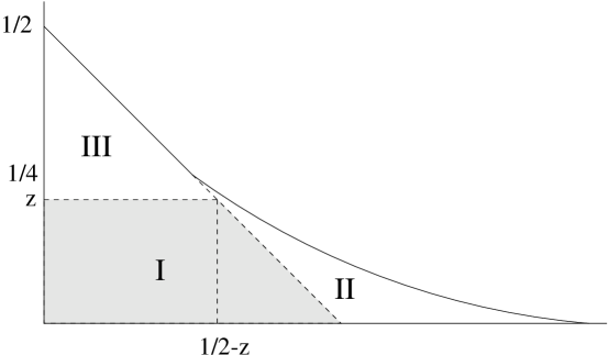
Figure 6: The reliability function for AWGN channel with infinite bandwidth

Since the error exponent for any given rate is a non-decreasing function of $B,$ a trivial observation we can make right away is that the tuple $(R_{crit}(1/B),z_{crit}(1/B))$ has to be below the infinite bandwidth reliability function. Equation (99) further tells us that it can not be in region III. Now we argue that $(R_{crit}(1/B),z_{crit}(1/B))$ can not be in region II either. If the tuple is in region II, we know the linear part of the random-coding exponent will intersect the infinite-bandwidth reliability function curve and thus for some communication rate, using a finite bandwidth $B/2$ is than using infinite bandwidth. This cannot be true and as a consequence, $(R_{crit}(1/B),z_{crit}(1/B))$ can only be in region I, which is the shaded region.

Next consider the random-coding exponent for rate $1/2-z.$ It is straightforward to see that

$$E_{r}(1/2-z,B)<z<E_{r}(1/2-z,\infty).$$

Combining this with our assumption, we know that the following equation can not be true:

$$\lim_{B\rightarrow\infty}E_{r}(1/2-z,B)=E_{r}(1/2-z,\infty).$$

However, it is well known that for any rate between $0$ and capacity, the random-coding exponent converges to the infinite-bandwidth error exponent as the bandwidth increases to infinity. Thus, we have a contradiction.

Appendix C Proof of Theorem 6

The error-exponent constraint gives us

$$pz=\sup_{0\leq\rho\leq 1}-\rho r+E_{o}(p,\rho),$$

which is equivalent to say the following

• For any $\rho\in[0,1],$ we always have

  $$pz\geq-\rho r+E_{o}(p,\rho).$$ (100)

• For any $\epsilon>0,$ we can find $\rho_{\epsilon},$ such that

  $$pz-\epsilon\leq-\rho_{\epsilon}r+E_{o}(p,\rho_{\epsilon}).$$ (101)

Similarly, what we want show is equivalent to the following

• For any $\rho\in[0,1],$ we always have

  $$r\geq-\frac{pz}{\rho}+\frac{E_{o}(p,\rho)}{\rho}.$$ (102)

• For any $\eta>0,$ we can find $\rho_{\eta},$ such that

  $$r-\eta\leq-\frac{pz}{\rho_{\eta}}+\frac{E_{o}(p,\rho_{\eta})}{\rho_{\eta}}.$$ (103)

It is easy to see that (102) follows directly from (100). Thus, it suffices to show (103) is true. To do this, first we construct an $\epsilon$ from $\eta$ as follows

$$\epsilon=\frac{pz\eta}{p-r+\eta}.$$ (104)

First we check that $\epsilon>0.$ This is true if we have $p>r.$ Note from the coding theorem, we know the largest rate available for reliable communication, which is defined as capacity, is equal to $\log(1+p)$ (nats per symbol) for AWGN channel. Hence, $r\leq c=log(1+p)\leq p.$

From (101), we know we could find a $\rho_{\epsilon}\in[0,1]$ such that

$$r\leq-\frac{pz}{\rho_{\epsilon}}+\frac{E_{o}(p,\rho_{\epsilon})}{\rho_{\epsilon}}+\frac{\epsilon}{\rho_{\epsilon}}.$$

Next we show $\frac{\epsilon}{\rho_{\epsilon}}\leq\eta.$

From Lemma 4, we know from (101 that

$$pz-\epsilon\leq\rho_{\epsilon}r+\frac{p\rho_{\epsilon}}{1+\rho_{\epsilon}}\leq-\rho_{\epsilon}r+p\rho_{\epsilon}=(p-r)\rho_{\epsilon}.$$

Hence, we must have

$$\rho_{\epsilon}\geq\frac{pz-\epsilon}{p-r}.$$

Thus,

$$\frac{\epsilon}{\rho_{\epsilon}}\leq\frac{\epsilon(p-r)}{pz-\epsilon}.$$

Use (104) to get

$$\frac{\epsilon}{\rho_{\epsilon}}\leq\eta.$$

In other words, for any $\eta>0,$ we simply use $\rho_{\eta}=\rho_{\epsilon},$ and we will have (103), which completes the proof of this theorem.

Appendix D Proof of $\lim_{p\rightarrow 0}\rho(p)=\rho^{*}$

We need to show that

$$\lim_{p\rightarrow 0}\rho(p)=\rho^{*},$$

where $\rho(p)$ is the optimizing $\rho$ for the following equation

$$\rho(p)=\arg\sup_{0\leq\rho\leq 1}-\frac{z}{\rho}+\frac{\dot{E}_{o}(0,\rho)}{\rho}+\frac{p\ddot{E}_{o}(0,\rho)}{2\rho},$$

and $\rho^{*}$ is defined as follows

$$\rho^{*}=\arg\sup_{0\leq\rho\leq 1}-\frac{z}{\rho}+\frac{1}{1+\rho}=\frac{\sqrt{z}}{1-\sqrt{z}}.$$

The assumption we can use here is that $\frac{\ddot{E}_{o}(0,\rho)}{\rho}$ is a continuous and bounded function in $\rho$ for $\rho\in[0,1].$ A direct consequence of this assumption is that as $p\rightarrow 0,$

$$\frac{\dot{E}_{o}(0,\rho)}{\rho}+\frac{p\ddot{E}_{o}(0,\rho)}{2\rho}\rightarrow\frac{\dot{E}_{o}(0,\rho)}{\rho}\quad\textsl{uniformly for ${\rho\in[0,1]}.$}$$ (105)

From the first-order calculation, we know that $\dot{E}_{o}(0,\rho)=\frac{\rho}{1+\rho}.$

We prove $\lim_{p\rightarrow 0}\rho(p)=\rho^{*}$ using a formal definition of the limit. For any $\epsilon_{0}>0,$ we show that we can find $\delta>0$ such that for all $p<\delta,$ we always have

$$|\rho(p)-\rho^{*}|<\epsilon_{0}.$$

To see this, define

$$\epsilon=(1-\sqrt{z})^{2}-\min(g(\rho^{*}-\epsilon_{0}),g(\rho^{*}+\epsilon_{0})),$$

where

$$g(\rho)=-\frac{z}{\rho}+\frac{1}{1+\rho}.$$

Now we use (105) here. For this $\epsilon$, we can find $\delta^{\prime}>0$ such that for any $\rho\in[0,1]$ and for all $p<\delta^{\prime},$ such that

$$\left|\frac{\dot{E}_{o}(0,\rho)}{\rho}+\frac{p\ddot{E}_{o}(0,\rho)}{2\rho}-\frac{1}{1+\rho}\right|\leq\frac{\epsilon}{2}.$$

Thus, we have

$$\sup_{0\leq\rho\leq 1}-\frac{z}{\rho}+\frac{\dot{E}_{o}(0,\rho)}{\rho}+\frac{p\ddot{E}_{o}(0,\rho)}{2\rho}>\sup_{0\leq\rho\leq 1}-\frac{z}{\rho}+\frac{1}{1+\rho}-\frac{\epsilon}{2}=(1-\sqrt{z})^{2}-\frac{\epsilon}{2}.$$

On the other hand, we also have

$$\sup_{0\leq\rho\leq 1}-\frac{z}{\rho}+\frac{\dot{E}_{o}(0,\rho)}{\rho}+\frac{p\ddot{E}_{o}(0,\rho)}{2\rho}$$

$$= -\frac{z}{\rho(p)}+\frac{1}{1+\rho(p)}+\frac{p\ddot{E}_{o}(0,\rho(p))}{2\rho(p)}$$

$$\leq g(\rho(p))+\frac{pM}{2},$$

where $M$ is the upper bound for $\frac{\ddot{E}_{o}(0,\rho)}{\rho}$ for $\rho\in[0,1].$ We choose $\delta=\min(\delta^{\prime},\frac{\epsilon}{M}),$ then for all $p<\delta,$ we have $\frac{pM}{2}\leq\frac{\epsilon}{2}.$ Further,

$$g(\rho(p))\geq(1-\sqrt{z})^{2}-\frac{\epsilon}{2}-\frac{pM}{2}\geq(1-\sqrt{z})^{2}-\epsilon.$$

From the definition of $\epsilon,$ we must have

$$|\rho(p)-\rho^{*}|<\epsilon_{0},$$

which finishes the proof of this part.

Appendix E Proof of Lemma 8

The first-order calculation gives us

$${\dot{E}}_{o}(0,\rho)=\frac{\rho}{1+\rho}.$$

Thus,

$$\frac{\frac{E_{o}(p,\rho)}{p\rho}-\frac{\dot{E}_{o}(0,\rho)}{\rho}}{p}$$

$$= \frac{-\ln\left(\inf_{\{q_{p}\}\in\tilde{\mathcal{G}}(p)}\inf_{\beta\geq 0}\int\alpha(y)^{1+\rho}dy\right)-\frac{\rho p}{1+\rho}}{\rho p^{2}}$$

$$= \frac{-\ln\left(e^{\frac{\rho p}{1+\rho}}\inf_{\{q_{p}\}\in\tilde{\mathcal{G}}(p)}\inf_{\beta\geq 0}\int\alpha(y)^{1+\rho}dy\right)}{\rho p^{2}}$$

$$= \frac{\ln\frac{1}{e^{\frac{\rho p}{1+\rho}}\inf_{\{q_{p}\}\in\tilde{\mathcal{G}}(p)}\inf_{\beta\geq 0}\int\alpha(y)^{1+\rho}dy}}{\rho p^{2}}$$

$$\leq \frac{-1+\frac{1}{e^{\frac{\rho p}{1+\rho}}\inf_{\{q_{p}\}\in\tilde{\mathcal{G}}(p)}\inf_{\beta\geq 0}\int\alpha(y)^{1+\rho}dy}}{\rho p^{2}}$$

$$= \frac{-e^{\frac{\rho p}{1+\rho}}\inf_{\{q_{p}\}\in\tilde{\mathcal{G}}(p)}\inf_{\beta\geq 0}\int\alpha(y)^{1+\rho}dy+1}{\rho p^{2}}\frac{1}{e^{\frac{\rho p}{1+\rho}}\inf_{\{q_{p}\}\in\tilde{\mathcal{G}}(p)}\inf_{\beta\geq 0}\int\alpha(y)^{1+\rho}dy}$$

$$\leq \frac{-e^{\frac{\rho p}{1+\rho}}\inf_{\{q_{p}\}\in\tilde{\mathcal{G}}(p)}\inf_{\beta\geq 0}\int\alpha(y)^{1+\rho}dy+1}{\rho p^{2}e^{\frac{\rho p}{1+\rho}}}$$

$$= \frac{-\inf_{\{q_{p}\}\in\tilde{\mathcal{G}}(p)}\inf_{\beta\geq 0}\int\alpha(y)^{1+\rho}dy+e^{-\frac{\rho p}{1+\rho}}}{\rho p^{2}}.$$

The inequality (E) is true because Lemma 4 implies

$$\inf_{\{q_{p}\}\in\tilde{\mathcal{G}}(p)}\inf_{\beta\geq 0}\int\alpha(y)^{1+\rho}dy=e^{-E_{o}(p,\rho)}\geq e^{-\frac{\rho p}{1+\rho}},$$

which leads to

$$-e^{\frac{\rho p}{1+\rho}}\inf_{\{q_{p}\}\in\tilde{\mathcal{G}}(p)}\inf_{\beta\geq 0}\int\alpha(y)^{1+\rho}dy+1\leq 0.$$

On the other hand,

$$\inf_{\{q_{p}\}\in\tilde{\mathcal{G}}(p)}\inf_{\beta\geq 0}\int\alpha(y)^{1+\rho}dy \leq \inf_{\{q_{p}\}\in\tilde{\mathcal{G}}(p)}\int\alpha(y)^{1+\rho}dy|_{\beta=0}$$

$$= \inf_{\{q_{p}\}\in\tilde{\mathcal{G}}(p)}\int\left(\sum_{k}q_{k}f(y|x_{k})^{\frac{1}{1+\rho}}\right)^{1+\rho}dy$$

$$\leq \inf_{\{q_{p}\}\in\tilde{\mathcal{G}}(p)}\int\left(\sum_{k}q_{k}f(y|x_{k})\right)dy$$

$$= 1.$$

These two bounds together give us (E).

Appendix F Proof of Lemma 11

First we check that

$$\int f_{w}(y)M^{2}(y)dy=E\left[e^{\beta^{*}(|x_{1}|^{2}+|x_{2}|^{2}-2p)}e^{-\theta(|x_{1}|^{2}+|x_{2}|^{2})}e^{\frac{2Re(x_{1}x_{2}^{*})}{(1+\rho^{*})^{2}}}\right],$$ (107)

and thus

$$\int f_{w}(y)T^{2}(y)dy = \int f_{w}(y)(M(y)-1)^{2}dy$$

$$= E\left[e^{\beta^{*}(|x_{1}|^{2}+|x_{2}|^{2}-2p)}e^{-\theta(|x_{1}|^{2}+|x_{2}|^{2})}\left(e^{\frac{2Re(x_{1}x_{2}^{*})}{(1+\rho^{*})^{2}}}-1\right)\right]+\left(E\left[e^{\beta^{*}(|x|^{2}-p)}e^{-\theta|x|^{2}}\right]-1\right)^{2}.$$

Since ${\tilde{E}}_{o}(p,q_{p},\rho)\geq{\tilde{E}}_{o}(p,QPSK,\rho),$ and

$${\tilde{E}}_{o}(p,q_{p},\rho)=-\ln\int\alpha(y)^{1+\rho}dy\leq-(1+\rho)\ln E\left[e^{\beta^{*}(|x|^{2}-p)}e^{-\theta|x|^{2}}\right],$$

we have

$$E\left[e^{\beta^{*}(|x|^{2}-p)}e^{-\theta|x|^{2}}\right]\leq e^{-\frac{{\tilde{E}}_{o}(p,QPSK,\rho)}{1+\rho}}.$$

As we will show later, $\frac{{\tilde{E}}_{o}(p,QPSk,\rho)}{\rho p}$ converges to $\frac{1}{1+\rho}$ uniformly. In other words, we can write ${\tilde{E}}_{o}(p,QPSK,\rho)$ as $\frac{\rho p}{1+\rho}+\rho\delta(p),$ where $\frac{\delta(p)}{p}$ goes to zero uniformly for all $\rho$ as $p$ goes to $0.$ Thus,

$$E\left[e^{\beta^{*}(|x|^{2}-p)}e^{-\theta|x|^{2}}\right]\leq e^{-\frac{\rho p}{(1+\rho)^{2}}+\frac{\rho}{1+\rho}\delta(p)}.$$

Note we should always have

$$E[\left[e^{\beta^{*}(|x|^{2}-p)}e^{-\theta|x|^{2}}\right]\leq 1,$$

for the optimizing $\beta^{*}.$ This can be seen by the following sequence of inequalities:

$$(E\left[e^{\beta^{*}(|x|^{2}-p)}e^{-\theta|x|^{2}}\right])^{1+\rho}$$

$$\leq \inf_{\beta\geq 0}\int\alpha^{1+\rho}dy$$

$$\leq \left.\int\alpha^{1+\rho}dy\right|_{\beta=0}$$

$$= \int\left(\sum_{k}q_{k}f(y|x_{k})^{\frac{1}{1+\rho}}\right)^{1+\rho}dy$$

$$\leq \int\sum_{k}q_{k}f(y|x_{k})dy$$

$$= 1.$$

Thus,

$$\left(E\left[e^{\beta^{*}(|x|^{2}-p)}e^{-\theta|x|^{2}}\right]-1\right)^{2}$$

$$\geq \left(e^{-\frac{\rho p}{(1+\rho)^{2}}+\frac{\rho}{1+\rho}\delta(p)}-1\right)^{2}$$

$$\geq \left\{\frac{\rho p}{(1+\rho)^{2}}-\frac{\rho}{1+\rho}\delta(p)-\frac{\left(\frac{\rho p}{(1+\rho)^{2}}-\frac{\rho}{1+\rho}\delta(p)\right)^{2}}{2}\right\}^{2}$$

$$= \theta^{2}p^{2}+\delta(p^{2}).$$

On the other hand, we have

$$E\left[e^{\beta^{*}(|x_{1}|^{2}+|x_{2}|^{2}-2p)}e^{-\theta(|x_{1}|^{2}+|x_{2}|^{2})}\left(e^{\frac{2Re(x_{1}x_{2}^{*})}{(1+\rho)^{2}}}-1\right)\right]$$

$$\geq E\left[e^{\beta^{*}(|x_{1}|^{2}+|x_{2}|^{2}-2p)}e^{-\theta(|x_{1}|^{2}+|x_{2}|^{2})}\frac{2Re(x_{1}x_{2}^{*})^{2}}{(1+\rho)^{4}}\right]$$

$$= E\left[e^{\beta^{*}(|x_{1}|^{2}+|x_{2}|^{2}-2p)}e^{-\theta(|x_{1}|^{2}+|x_{2}|^{2})}\frac{2(x_{1r}^{2}x_{2r}^{2}+x_{1c}^{2}x_{2c}^{2}+2x_{1r}x_{1c}x_{2r}x_{2c})}{(1+\rho)^{4}}\right]$$

$$\geq \frac{2}{(1+\rho)^{4}}\left\{(E[e^{\beta^{*}(|x_{1}|^{2}-p)}e^{-\theta|x_{1}|^{2}}x_{1r}^{2}])^{2}+(E[e^{\beta^{*}(|x_{1}|^{2}-p)}e^{-\theta|x_{1}|^{2}}x_{1c}^{2}])^{2}\right\}$$

$$\geq \frac{\left(E[e^{\beta^{*}(|x_{1}|^{2}-p)}e^{-\theta|x_{1}|^{2}}(x_{1r}^{2}+x_{1c}^{2})]\right)^{2}}{(1+\rho)^{4}}$$

$$= \frac{\left(E[e^{\beta^{*}(|x_{1}|^{2}-p)}e^{-\theta|x_{1}|^{2}}|x_{1}|^{2}]\right)^{2}}{(1+\rho)^{4}}$$

$$\geq \frac{\left(E[(1+\beta^{*}(|x_{1}|^{2}-p)-\theta|x_{1}|^{2})|x_{1}|^{2}]\right)^{2}}{(1+\rho)^{4}}$$

$$\geq \frac{\left(p-\theta E[|x_{1}|^{4}]\right)^{2}}{(1+\rho)^{4}}$$

$$\geq \frac{\left(p-\theta K_{m}^{2}p^{1+2\alpha}\right)^{2}}{(1+\rho)^{4}}$$

$$\geq \frac{p^{2}-2\theta K_{m}^{2}p^{2+2\alpha}}{(1+\rho)^{4}}$$

$$= \frac{p^{2}}{(1+\rho)^{4}}+\delta(p^{2}).$$

In the above equations, $x_{ir}$, $x_{ic}$ denote the real part and imaginary part of the random variable $x_{i}$, $i=1,2$.

Appendix G Proof of Lemma 12

To prove Lemma 12, we first establish two other lemmas. The first lemma shows that we can restrict ourselves to considering distributions which are symmetric around $0.$ Define $\Gamma(q)=\int\alpha(y)^{1+\rho}dy$.

Lemma 19

Given any distribution $q(x)\in{\tilde{\mathcal{F}}}(p),$ we can find a symmetric distribution $q_{e}(x)\in{\tilde{\mathcal{F}}}(p),$ i.e., $q_{e}(x)=q_{e}(-x)\enskip\forall x,$ such that $\Gamma(q_{e})\leq\Gamma(q).$

Proof: We first compute $\Gamma(\cdot)$ for $q(-x)$ and show that it is the same as $\Gamma(q).$

$$\int\left(\int q(-x)e^{\beta(|x|^{2}-p)}f_{w}(y-x)^{\frac{1}{1+\rho}}dx\right)^{1+\rho}dy$$

$$= \int\left(\int q(x)e^{\beta(|-x|^{2}-p)}f_{w}(y+x)^{\frac{1}{1+\rho}}dx\right)^{1+\rho}dy$$

$$= \int\left(\int q(x)e^{\beta(|x|^{2}-p)}f_{w}(-y+x)^{\frac{1}{1+\rho}}dx\right)^{1+\rho}dy$$

$$= \int\left(\int q(x)e^{\beta(|x|^{2}-p)}f_{w}(y-x)^{\frac{1}{1+\rho}}dx\right)^{1+\rho}dy$$

$$= \Gamma(q).$$

For $\rho\in[0,1]$, it is easy to see that $\int\alpha(y)^{1+\rho}dy$ is a convex function of $q(x)$ for a fixed $\beta$ . Thus if we choose $q_{e}(x)=\frac{1}{2}(q(x)+q(-x))$, the power constraint will be still valid and we have

$$\Gamma(q_{e}(x))=\int\left(\int q_{e}(x)e^{\beta(|x|^{2}-p)}f_{w}(y-x)^{\frac{1}{1+\rho}}dx\right)^{1+\rho}dy\leq\frac{1}{2}(\Gamma(q)+\Gamma(q))=\Gamma(q).$$

$\diamond$

The second lemma provides an upper bound for $E[e^{\beta^{*}(|x|^{2}-p)}e^{-\theta|x|^{2}}|x|^{2}],$ which is a key term in the proof of Lemma 12.

Lemma 20

For any input distribution $\{q_{p}\}$ which has mean variance $p,$ let $\beta^{*}$ be the optimizing $\beta$ as in (59). We must have

$$E[e^{\beta^{*}(|x|^{2}-p)}e^{-\theta|x|^{2}}|x|^{2}]\leq pe^{\theta p}.$$ (108)

Proof: Denote

$$h(\beta)=\int\left(\sum q_{k}e^{\beta(|x_{k}|^{2}-p)}f(y|x_{k})^{\frac{1}{1+\rho}}\right)^{1+\rho}dy.$$

If $\beta^{*}$ is the optimizing $\beta,$ applying the Kuch-Tucker condition here, we must have

$$\beta^{*}h^{\prime}(\beta^{*})=0,$$

which yields $\beta^{*}=0$ or

$$\int\left(\sum_{k}q_{k}e^{\beta^{*}(|x_{k}|^{2}-p)}f(y|x_{k})^{\frac{1}{1+\rho}}\right)^{\rho}\sum_{k}q_{k}e^{\beta^{*}(|x_{k}|^{2}-p)}f(y|x_{k})^{\frac{1}{1+\rho}}(|x_{k}|^{2}-p)dy=0,$$

which can be simplified as

$$p\int\alpha(y)^{1+\rho}dy=\int\alpha(y)^{\rho}\gamma(y)dy.$$ (109)

Here we let

$$\alpha(y) = \sum_{k}q_{k}e^{\beta^{*}(|x_{k}|^{2}-p)}f(y|x_{k})^{\frac{1}{1+\rho}};$$

$$\gamma(y) = \sum_{k}q_{k}e^{\beta^{*}(|x_{k}|^{2}-p)}f(y|x_{k})^{\frac{1}{1+\rho}}|x_{k}|^{2}.$$

If $\beta^{*}=0,$ (108) is trivial.

If $\beta^{*}>0,$ we derive (108) using (109). Note that

$$\int\alpha(y)^{\rho}\gamma(y)dy \geq \int\sum_{k}q_{k}e^{\beta^{*}\rho(|x_{k}|^{2}-p)}f(y|x_{k})^{\frac{\rho}{1+\rho}}\gamma(y)dy$$

$$= \sum_{k}q_{k}e^{\beta^{*}\rho(|x_{k}|^{2}-p)}\sum_{l}q_{l}e^{\beta^{*}(|x_{l}|^{2}-p)}|x_{l}|^{2}\int f(y|x_{k})^{\frac{\rho}{1+\rho}}f(y|x_{l})^{\frac{1}{1+\rho}}dy$$

$$= \sum_{l}q_{l}e^{\beta^{*}(|x_{l}|^{2}-p)}|x_{l}|^{2}\sum_{k}q_{k}e^{\beta^{*}\rho(|x_{k}|^{2}-p)}e^{-\theta|x_{k}-x_{l}|^{2}}$$

$$\geq \sum_{l}q_{l}e^{\beta^{*}(|x_{l}|^{2}-p)}|x_{l}|^{2}e^{\sum_{k}q_{k}\{\beta^{*}\rho(|x_{k}|^{2}-p)-\theta|x_{k}-x_{l}|^{2}\}}$$

$$\geq \sum_{l}q_{l}e^{\beta^{*}(|x_{l}|^{2}-p)}|x_{l}|^{2}e^{-\theta p}e^{-\theta|x_{l}|^{2}}$$

$$= e^{-\theta p}E[e^{\beta^{*}(|x|^{2}-p)}e^{-\theta|x|^{2}}|x|^{2}].$$

On the other hand, as we have shown before,

$$\int\alpha(y)^{1+\rho}dy = \inf_{\beta\geq 0}\int\left(\sum q_{k}e^{\beta(|x_{k}|^{2}-p)}f(y|x_{k})^{\frac{1}{1+\rho}}\right)^{1+\rho}dy\leq 1.$$

Thus, we must have

$$E[e^{\beta^{*}(|x|^{2}-p)}e^{-\theta|x|^{2}}|x|^{2}]\leq e^{\theta p}\int\alpha(y)^{\rho}\gamma(y)dy=pe^{\theta p}\int\alpha(y)^{1+\rho}dy\leq pe^{\theta p}.$$ (110)

$\diamond$

Now we prove Lemma 12.

$$\int f_{w}(y)T^{3}(y)dy = \int f_{w}(y)(M(y)-1)^{3}dy$$

$$= \int f_{w}(y)(M^{3}(y)-3M^{2}(y)+3M(y)-1)dy.$$

It is easy to check that

$$\int f_{w}(y)M(y)dy = E\left[e^{\beta^{*}(|x_{1}|^{2}-p)}e^{-\theta|x_{1}|^{2}}\right];$$

$$\int f_{w}(y)M^{2}(y)dy = E\left[e^{\beta^{*}(|x_{1}|^{2}+|x_{2}|^{2}-2p)}e^{-\theta(|x_{1}|^{2}+|x_{2}|^{2})}e^{\frac{2Re(x_{1}x_{2}^{*})}{(1+\rho)^{2}}}\right];$$

$$\int f_{w}(y)M^{3}(y)dy = E\left[e^{\beta^{*}(|x_{1}|^{2}+|x_{2}|^{2}+|x_{3}|^{2}-3p)}e^{-\theta(|x_{1}|^{2}+|x_{2}|^{2}+|x_{3}|^{2})}e^{\frac{2Re(x_{1}x_{2}^{*}+x_{1}x_{3}^{*}+x_{2}x_{3}^{*})}{(1+\rho)^{2}}}\right],$$

where $x_{1}$, $x_{2}$ and $x_{3}$ are i.i.d. random variables with distribution $\{q_{p}(x)\}.$ Thus, after some manipulations, we have

$$\int f_{w}(y)T^{3}(y)dy=\left(E\left[e^{\beta^{*}(|x_{1}|^{2}-p)}e^{-\theta|x_{1}|^{2}}\right]-1\right)^{3}$$

$$-3E\left[e^{\beta^{*}(|x_{1}|^{2}+|x_{2}|^{2}-2p)}e^{-\theta(|x_{1}|^{2}+|x_{2}|^{2})}\left(e^{\frac{2Re(x_{1}x_{2}^{*})}{(1+\rho)^{2}}}-1\right)\right]$$

$$+E\left[e^{\beta^{*}(|x_{1}|^{2}+|x_{2}|^{2}+|x_{3}|^{2}-3p)}e^{-\theta(|x_{1}|^{2}+|x_{2}|^{2}+|x_{3}|^{2})}\left(e^{\frac{2Re(x_{1}x_{2}^{*}+x_{1}x_{3}^{*}+x_{2}x_{3}^{*})}{(1+\rho)^{2}}}-1\right)\right].$$ (111)

From the proof in Lemma 11, we know

$$e^{-\theta p}-1\leq E\left[e^{\beta^{*}(|x_{1}|^{2}-p)}e^{-\theta|x_{1}|^{2}}\right]-1\leq 0,$$

and thus, we must have

$$\left|E\left[\exp\left\{(\beta^{*}-\theta)(|x_{1}|^{2}-p)\right\}\right]e^{-\theta p}-1\right|^{3}\leq(1-e^{-\theta p})^{3}\leq\theta^{3}p^{3}.$$

On the other hand, we expand the second and third term in the RHS of (111) as follows:

$$E\left[e^{\beta^{*}(|x_{1}|^{2}+|x_{2}|^{2}-2p)}e^{-\theta(|x_{1}|^{2}+|x_{2}|^{2})}\left(e^{\frac{2Re(x_{1}x_{2}^{*})}{(1+\rho)^{2}}}-1\right)\right]$$

$$= \sum_{k=1}^{\infty}E\left[e^{\beta^{*}(|x_{1}|^{2}+|x_{2}|^{2}-2p)}e^{-\theta(|x_{1}|^{2}+|x_{2}|^{2})}\frac{(2Re(x_{1}x_{2}^{*}))^{k}}{(1+\rho)^{2k}k!}\right],$$ (112)

and

$$E\left[e^{\beta^{*}(|x_{1}|^{2}+|x_{2}|^{2}+|x_{3}|^{2}-3p)}e^{-\theta(|x_{1}|^{2}+|x_{2}|^{2}+|x_{3}|^{2})}\left(e^{\frac{2Re(x_{1}x_{2}^{*}+x_{1}x_{3}^{*}+x_{2}x_{3}^{*})}{(1+\rho)^{2}}}-1\right)\right]$$

$$= \sum_{k=1}^{\infty}E\left[e^{\beta^{*}(|x_{1}|^{2}+|x_{2}|^{2}+|x_{3}|^{2}-3p)}e^{-\theta(|x_{1}|^{2}+|x_{2}|^{2}+|x_{3}|^{2})}\frac{2^{k}(Re(x_{1}x_{2}^{*})+Re(x_{1}x_{3}^{*})+Re(x_{2}x_{3}^{*}))^{k}}{(1+\rho)^{2k}k!}\right]$$

$$= \sum_{k=1}^{\infty}\sum_{l+m+n=k}E\left[e^{\beta^{*}(|x_{1}|^{2}+|x_{2}|^{2}+|x_{3}|^{2}-3p)}e^{-\theta(|x_{1}|^{2}+|x_{2}|^{2}+|x_{3}|^{2})}{\frac{2^{k}C_{lmn}^{(k)}Re(x_{1}x_{2}^{*})^{l}Re(x_{1}x_{3}^{*})^{m}Re(x_{2}x_{3}^{*})^{n}}{(1+\rho)^{2k}k!}}\right],$$

where $C_{lmn}^{(k)}$ is a non-negative constant independent of $p.$

It is straightforward to check to following, using the above two expansions:

$$E\left[e^{\beta^{*}(|x_{1}|^{2}+|x_{2}|^{2}+|x_{3}|^{2}-3p)}e^{-\theta(|x_{1}|^{2}+|x_{2}|^{2}+|x_{3}|^{2})}\left(e^{\frac{2Re(x_{1}x_{2}^{*}+x_{1}x_{3}^{*}+x_{2}x_{3}^{*})}{(1+\rho)^{2}}}-1\right)\right]$$

$$-3E\left[e^{\beta^{*}(|x_{1}|^{2}+|x_{2}|^{2}-2p)}e^{-\theta(|x_{1}|^{2}+|x_{2}|^{2})}\left(e^{\frac{2Re(x_{1}x_{2}^{*})}{(1+\rho)^{2}}}-1\right)\right]$$

$$= \sum_{k=1}^{\infty}\sum_{\begin{array}[]{l}l+m+n=k;\\ l,m,n<k\end{array}}E\left[e^{\beta^{*}(|x_{1}|^{2}+|x_{2}|^{2}+|x_{3}|^{2}-3p)}e^{-\theta(|x_{1}|^{2}+|x_{2}|^{2}+|x_{3}|^{2})}{\frac{2^{k}C_{lmn}^{(k)}Re(x_{1}x_{2}^{*})^{l}Re(x_{1}x_{3}^{*})^{m}Re(x_{2}x_{3}^{*})^{n}}{(1+\rho)^{2k}k!}}\right]$$

$$+3\sum_{k=1}^{\infty}E\left[e^{\beta^{*}(|x_{1}|^{2}+|x_{2}|^{2}-2p)}e^{-\theta(|x_{1}|^{2}+|x_{2}|^{2})}\frac{(2Re(x_{1}x_{2}^{*}))^{k}}{(1+\rho)^{2k}k!}\right]\left\{E[e^{\beta^{*}(|x_{3}|^{2}-p)}e^{-\theta|x_{3}|^{2}}]-1\right\}.$$

Next, we bound the two terms above separately, using the bound that $Re(z)\leq|z|.$ Note that for symmetric distributions, it is easy to see that all the $k$ odd terms will vanish. Thus, we can remove the term with $k=1.$

$$\left|\sum_{k=1}^{\infty}E\left[e^{\beta^{*}(|x_{1}|^{2}+|x_{2}|^{2}-2p)}e^{-\theta(|x_{1}|^{2}+|x_{2}|^{2})}\frac{(2Re(x_{1}x_{2}^{*}))^{k}}{(1+\rho)^{2k}k!}\right]\left\{E[e^{\beta^{*}(|x_{3}|^{2}-p)}e^{-\theta|x_{3}|^{2}}]-1\right\}\right|$$

$$\leq \sum_{k=2}^{\infty}\left|E\left[e^{\beta^{*}(|x_{1}|^{2}+|x_{2}|^{2}-2p)}e^{-\theta(|x_{1}|^{2}+|x_{2}|^{2})}\frac{(2Re(x_{1}x_{2}^{*}))^{k}}{(1+\rho)^{2k}k!}\right]\right|\left|\left\{E[e^{\beta^{*}(|x_{3}|^{2}-p)}e^{-\theta|x_{3}|^{2}}]-1\right\}\right|$$

$$\leq \sum_{k=2}^{\infty}E\left[e^{\beta^{*}(|x_{1}|^{2}+|x_{2}|^{2}-2p)}e^{-\theta(|x_{1}|^{2}+|x_{2}|^{2})}\frac{2^{k}|x_{1}|^{k}|x_{2}|^{k}}{(1+\rho)^{2k}k!}\right](1-e^{-\theta p})$$

$$\leq \theta p\sum_{k=2}^{\infty}\frac{2^{k}}{(1+\rho)^{2k}k!}\left(E\left[e^{\beta^{*}(|x_{1}|^{2}-p)}e^{-\theta|x_{1}|^{2}}|x_{1}|^{k}\right]\right)^{2}$$

$$\leq \theta p\sum_{k=2}^{\infty}\frac{2^{k}(K_{m}p^{\alpha})^{2(k-2)}}{(1+\rho)^{2k}k!}\left(E\left[e^{\beta^{*}(|x_{1}|^{2}-p)}e^{-\theta|x_{1}|^{2}}|x_{1}|^{2}\right]\right)^{2}$$

$$\leq 4\theta pe^{2K_{m}^{2}}\left(E\left[e^{\beta^{*}(|x_{1}|^{2}-p)}e^{-\theta|x_{1}|^{2}}|x_{1}|^{2}\right]\right)^{2}$$

$$\leq 4\theta e^{2\theta p}e^{2K_{m}^{2}}p^{3}.$$

Similarly, for the other term, we can also remove the term where $k$ is odd. Actually, we can do more. For example, when $k=2,$ since at least two of $l,m,n$ are required to be non-zero, we must have two of them are $1,$ while the other is $0.$ It can be easily seen the contribution of this term is also zero, for symmetric distributions. Thus, we remove the terms for both $k=1$ and $k=2.$

$$\sum_{k=1}^{\infty}\sum_{\begin{array}[]{l}l+m+n=k;\\ l,m,n<k\end{array}}E\left[e^{\beta^{*}(|x_{1}|^{2}+|x_{2}|^{2}+|x_{3}|^{2}-3p)}e^{-\theta(|x_{1}|^{2}+|x_{2}|^{2}+|x_{3}|^{2})}{\frac{2^{k}C_{lmn}^{(k)}Re(x_{1}x_{2}^{*})^{l}Re(x_{1}x_{3}^{*})^{m}Re(x_{2}x_{3}^{*})^{n}}{(1+\rho)^{2k}k!}}\right]$$

$$\leq \sum_{k=3}^{\infty}\frac{2^{k}}{(1+\rho)^{2k}k!}\sum_{\begin{array}[]{l}l+m+n=k;\\ l,m,n<k\end{array}}C_{lmn}^{(k)}E\left[e^{\beta^{*}(|x_{1}|^{2}+|x_{2}|^{2}+|x_{3}|^{2}-3p)}e^{-\theta(|x_{1}|^{2}+|x_{2}|^{2}+|x_{3}|^{2})}|x_{1}|^{l+m}|x_{2}|^{m+n}|x_{3}|^{m+n}\right]$$

$$= \sum_{k=3}^{\infty}\frac{2^{k}}{(1+\rho)^{2k}k!}\sum_{\begin{array}[]{l}l+m+n=k;\\ l,m,n<k\end{array}}C_{lmn}^{(k)}E\left[e^{\beta^{*}(|x_{1}|^{2}-p)}e^{-\theta|x_{1}|^{2}}|x_{1}|^{l+m}\right]*$$

$$E\left[e^{\beta^{*}(|x_{2}^{2}-p)}e^{-\theta|x_{2}|^{2}}|x_{2}|^{l+n}\right]*E\left[e^{\beta^{*}(|x_{3}|^{2}-p)}e^{-\theta|x_{3}|^{2}}|x_{3}|^{m+n}\right]$$

$$\leq \sum_{k=3}^{\infty}\frac{2^{k}K_{m}^{2k-6}}{(1+\rho)^{2k}k!}\sum_{\begin{array}[]{l}l+m+n=k;\\ l,m,n<k\end{array}}C_{lmn}^{(k)}\left(E\left[e^{\beta^{*}(|x_{1}|^{2}-p)}e^{-\theta|x_{1}|^{2}}|x_{1}|^{2}\right]\right)^{3}$$

$$\leq \sum_{k=3}^{\infty}\frac{6^{k}K_{m}^{2k-6}}{(1+\rho)^{2k}k!}\left(E\left[e^{\beta^{*}(|x_{1}|^{2}-p)}e^{-\theta|x_{1}|^{2}}|x_{1}|^{2}\right]\right)^{3}$$

$$\leq 216e^{6K_{m}^{2}}\left(E\left[e^{\beta^{*}(|x_{1}|^{2}-p)}e^{-\theta|x_{1}|^{2}}|x_{1}|^{2}\right]\right)^{3}$$

$$\leq 216e^{6K_{m}^{2}}e^{3\theta p}p^{3}.$$

Combining all these bounds, we have

$$\left|\int f_{w}(y)T^{3}(y)dy\right| \leq \theta^{3}p^{3}+12\theta e^{2\theta p}e^{2K_{m}^{2}}p^{3}+216e^{6K_{m}^{2}}e^{3\theta p}p^{3}$$

$$\leq Ce^{3\theta p}p^{3},$$

where $C$ is a constant, which is independent of $\rho$ and independent of the choice of input distributions, as far as it is in ${\tilde{\mathcal{F}}}(p).$

Appendix H Proof of Lemma 7

To show this, we need to check (50) for a sequence of mean-zero input distribution $q_{p}\in{\tilde{\mathcal{F}}}(p).$ Since it is always true that

$$\limsup_{p\rightarrow 0}\frac{{\tilde{E}}_{o}(p,q_{p},\rho^{*})}{p}\leq\frac{\rho^{*}}{1+\rho^{*}},$$

it suffices to show that

$$\liminf_{p\rightarrow 0}\frac{{\tilde{E}}_{o}(p,q_{p},\rho^{*})}{p}\geq\frac{\rho^{*}}{1+\rho^{*}}.$$

Note

$${\tilde{E}}_{o}(p,q_{p},\rho^{*}) = \sup_{\beta\geq 0}-\ln\int\alpha(y)^{1+\rho^{*}}dy$$

$$= \sup_{\beta\geq 0}-\ln\int f_{w}(y)(1+T(y))^{1+\rho^{*}}dy.$$

To achieve a lower bound, we choose $\beta=\theta=\frac{\rho^{*}}{1+\rho^{*}}.$ Further, we use the following inequality

$$(1+t)^{1+\rho^{*}}\leq 1+(1+\rho^{*})t+\frac{\rho^{*}(1+\rho^{*})}{2}t^{2}.$$

This leads to

$${\tilde{E}}_{o}(p,q_{p},\rho^{*})\geq-\ln\int f_{w}(y)(1+(1+\rho^{*})T(y)+\frac{\rho^{*}(1+\rho^{*})}{2}T^{2}(y))dy.$$

When $\beta=\theta,$ it can be shown that

$$\int f_{w}(y)(1+(1+\rho^{*})T(y))dy=-\rho^{*}+(1+\rho^{*})e^{-\theta p},$$

and

$$\int f_{w}(y)T^{2}(y)dy=1-2e^{-\theta p}+E\left[e^{\frac{2Re(x_{1}x_{2}^{*})}{(1+\rho^{*})^{2}}}\right]e^{-2\theta p},$$

where $x_{1}$ and $x_{2}$ are i.i.d random variables distributed according to $q_{p}(x).$

Next we claim

$$\lim_{p\rightarrow 0}\frac{\int f_{w}(y)T^{2}(y)dy}{p}=0.$$

Since $\lim_{p\rightarrow 0}\frac{(1-e^{-\theta p})^{2}}{p}=0,$ it suffices to show

$$\lim_{p\rightarrow 0}\frac{E\left[e^{\frac{2Re(x_{1}x_{2}^{*})}{(1+\rho^{*})^{2}}}\right]-1}{p}=0.$$

Using the assumption that $q_{p}(x)$ is symmetric around $0$ and

$$|x|_{max}<K_{m}p^{\alpha},$$

we can show this following a similar procedure as in the proof of Lemma 12.

Thus, we have

$$\liminf_{p\rightarrow 0}\frac{{\tilde{E}}_{o}(p,q_{p},\rho^{*})}{p} \geq \liminf_{p\rightarrow 0}\frac{-\ln(-\rho^{*}+(1+\rho^{*})e^{-\theta p}+o(p))}{p}$$

$$= \liminf_{p\rightarrow 0}\frac{-\ln(1-\frac{\rho^{*}p}{1+\rho^{*}}+o(p))}{p}$$

$$= \frac{\rho^{*}}{1+\rho^{*}}.$$

Appendix I BPSK and QPSK for AWGN channels

Since for both BPSK and QPSK, we have $|x|^{2}=p$ with probability $1$, the power constraint parameter $\beta$ does not play a role here and ${\tilde{E}}_{o}(p,q_{p},\rho)$ can be simplified to

$${\tilde{E}}_{o}(p,q_{p},\rho)=-\ln\int\alpha(y)^{1+\rho}dy,$$

with

$$\alpha(y)=\int q_{p}(x)f_{w}(y|x)^{\frac{1}{1+\rho}}dx.$$

Again, we use the two inequalities which have been very helpful to us in the general first and second order calculations:

$$(1+t)^{1+\rho} \leq 1+(1+\rho)t+\frac{\rho(1+\rho)}{2}t^{2};$$ (118)

$$(1+t)^{1+\rho} \geq 1+(1+\rho)t+\frac{\rho(1+\rho)}{2}t^{2}-\frac{\rho(1+\rho)(1-\rho)}{6}t^{3}.$$ (119)

We write $\int\alpha(y)dy$ as follows

$$\int\alpha(y)dy=\int f_{w}(y)(1+T(y))^{1+\rho}dy,$$ (120)

where $T(y)$ denotes

$$T(y)=\sum_{k}q_{k}\left(\frac{f(y|x)}{f(y|0)}\right)^{\frac{1}{1+\rho}}-1.$$

It is easy to check for BPSK or QPSK, we have

$$\int f_{w}(y)T(y)dy = e^{-\theta p}-1;$$

$$\int f_{w}(y)T^{2}(y)dy = (e^{-\theta p}-1)^{2}+e^{-2\theta p}E[e^{\frac{2Re(x_{1}x_{2}^{*})}{(1+\rho)^{2}}}-1];$$

$$\int f_{w}(y)T^{3}(y)dy = (e^{-\theta p}-1)^{3}+e^{-3\theta p}E[e^{\frac{2Re(x_{1}x_{2}^{*})+2Re(x_{1}x_{3}^{*})+2Re(x_{2}x_{3}^{*})}{(1+\rho)^{2}}}-1]-3e^{-2\theta p}E[e^{\frac{2Re(x_{1}x_{2}^{*})}{(1+\rho)^{2}}}-1].$$

Further, for BPSK, we can calculate that

$$E[e^{\frac{2Re(x_{1}x_{2}^{*})}{(1+\rho)^{2}}}]=\frac{1}{2}\left(e^{\frac{2p}{(1+\rho)^{2}}}+e^{-\frac{2p}{(1+\rho)^{2}}}-2\right)=1+\frac{2p^{2}}{(1+\rho)^{4}}+\delta(p^{2}).$$ (121)

and

$$E[e^{\frac{2Re(x_{1}x_{2}^{*})}{(1+\rho)^{2}}}] = 1+\frac{2p^{2}}{(1+\rho)^{4}}+\delta(p^{2});$$

$$E[e^{\frac{2Re(x_{1}x_{2}^{*})+2Re(x_{1}x_{3}^{*})+2Re(x_{2}x_{3}^{*})}{(1+\rho)^{2}}}] = 1+\frac{6p^{2}}{(1+\rho)^{4}}+\delta(p^{2}),$$

which further yield an upper bound and lower bound for $\int\alpha(y)dy,$

$$\int\alpha(y)dy \leq 1+(1+\rho)\int f_{w}(y)T(y)dy+\frac{\rho(1+\rho)}{2}\int f_{w}(y)T^{2}(y)dy$$

$$= 1+(1+\rho)(e^{-\theta p}-1)+\frac{\rho(1+\rho)}{2}\left\{(e^{-\theta p}-1)^{2}+\frac{2p^{2}}{(1+\rho)^{4}}+\delta(p^{2})\right\}$$

$$\leq 1+(1+\rho)(-\theta p+\frac{\theta^{2}p^{2}}{2})+\frac{\rho(1+\rho)}{2}\left\{\theta^{2}p^{2}+\frac{2p^{2}}{(1+\rho)^{4}}+\delta(p^{2})\right\}$$

$$= 1-\frac{\rho}{1+\rho}p+\frac{\rho^{3}+\rho^{2}+2\rho}{(1+\rho)^{3}}\frac{p^{2}}{2}+\rho\delta(p^{2});$$

$$\int\alpha(y)dy \geq 1+(1+\rho)\int f_{w}(y)T(y)dy+\frac{\rho(1+\rho)}{2}\int f_{w}(y)T^{2}(y)dy-\frac{\rho(1+\rho)(1-\rho)}{6}\int f_{w}(y)T^{3}(y)dy$$

$$= 1+(1+\rho)(e^{-\theta p}-1)+\frac{\rho(1+\rho)}{2}\left\{(e^{-\theta p}-1)^{2}+\frac{2p^{2}}{(1+\rho)^{4}}+\delta(p^{2})\right\}+\rho\delta(p^{2})$$

$$\geq 1+(1+\rho)(-\theta p+\frac{\theta^{2}p^{2}}{2}-\frac{\theta^{3}p^{3}}{6})+\frac{\rho(1+\rho)}{2}\left\{(-\theta p+\frac{\theta^{2}p^{2}}{2})^{2}+\frac{2p^{2}}{(1+\rho)^{4}}+\delta(p^{2})\right\}+\rho\delta(p^{2})$$

$$= 1-\frac{\rho}{1+\rho}p+\frac{\rho^{3}+\rho^{2}+2\rho}{(1+\rho)^{3}}\frac{p^{2}}{2}+\rho\delta(p^{2}).$$

In other words, we must have

$$\int\alpha(y)dy=1-\frac{\rho}{1+\rho}p+\frac{\rho^{3}+\rho^{2}+2\rho}{(1+\rho)^{3}}\frac{p^{2}}{2}+\rho\delta(p^{2}).$$

Thus,

$$\tilde{r}(p) = \sup_{0\leq\rho\leq 1}-\frac{pz}{\rho}+\frac{{\tilde{E}}_{o}(p,BPSK,\rho)}{\rho}$$

$$= \sup_{0\leq\rho\leq 1}-\frac{pz}{\rho}+\frac{-\ln\int\alpha(y)dy}{\rho}$$

$$= \sup_{0\leq\rho\leq 1}-\frac{pz}{\rho}+\frac{p}{1+\rho}-\frac{p^{2}}{(1+\rho)^{3}}+\delta(p^{2}).$$

From here, it is easy to check that

$$\frac{{\tilde{E}}_{o}(p,BPSK,\rho)}{p\rho}\rightarrow\frac{1}{1+\rho}$$

uniformly for $0\leq\rho\leq 1$ as $p\rightarrow 0.$ Further,

$$\frac{\frac{{\tilde{E}}_{o}(p,BPSK,\rho)}{p\rho}-\frac{1}{1+\rho}}{p}\rightarrow-\frac{2}{(1+\rho)^{3}}.$$

From Theorem 7 and Theorem 8, we know this implies

$$\dot{\tilde{r}}(0) = \sup_{0\leq\rho\leq 1}-\frac{z}{\rho}+\frac{1}{1+\rho}=(1-\sqrt{z})^{2};$$

$$\ddot{\tilde{r}}(0) = \frac{\ddot{{\tilde{E}}_{o}}(0,BPSK,\rho^{*})}{\rho^{*}}=-\frac{2}{(1+\rho^{*})^{3}}=-2(1-\sqrt{z})^{3}.$$

Therefore, BPSK is first-order optimal but not second-order optimal.

The QPSK calculations are very similar to the BPSK calculations and we can show that for QPSK

$$\dot{\tilde{r}}(0) = \sup_{0\leq\rho\leq 1}-\frac{z}{\rho}+\frac{1}{1+\rho}=(1-\sqrt{z})^{2};$$

$$\ddot{\tilde{r}}(0) = \frac{\ddot{{\tilde{E}}_{o}}(0,QPSK,\rho^{*})}{\rho^{*}}=-(1-\sqrt{z})^{3},$$

which implies that QPSK is near-optimal.

Appendix J Proof of Lemma 16

It suffices to check (80) for this choice of input distributions. When $q_{W_{c}}$ has i.i.d. entries, we have the following:

$$E_{o}(P,q_{W_{c}},\rho^{*},W_{c}) \geq E_{o}(P,q_{W_{c}},\rho^{*},W_{c})|_{\beta=\theta}$$ (122)

$$= -\ln E_{H}\left[\exp\{-DE_{o}^{NF}(\frac{P|H|^{2}}{W_{c}},q,\rho^{*})|_{\beta=\theta}\}\right],$$

where $\theta=\frac{\rho^{*}}{(1+\rho^{*})^{2}}.$ Following Appendix H , we know that if $q$ is symmetric around $0,$ we have

$$\liminf_{p\rightarrow 0}\frac{E_{o}^{NF}(p,q,\rho^{*})|_{\beta=\theta}}{p}\geq\frac{\rho^{*}}{1+\rho^{*}}.$$ (123)

From Lemma 4,

$$\frac{E_{o}^{NF}(p,q,\rho^{*})|_{\beta=\theta}}{p}\leq\frac{\rho^{*}}{1+\rho^{*}}.$$

Thus, actually, if we take $\beta=\theta,$ the limit of $\frac{E_{o}^{NF}(p,q,\rho^{*})|_{\beta=\theta}}{p}$ exists and is equal to $\frac{\rho^{*}}{1+\rho^{*}}.$

This result also implies

$$\lim_{W_{c}\rightarrow\infty}DE_{o}^{NF}(\frac{P|H|^{2}}{W_{c}},q,\rho^{*})|_{\beta=\theta}=\frac{\rho^{*}P|H|^{2}}{1+\rho^{*}}\quad\textsl{a.e. for $|H|^{2}\in R^{+}.$}$$

On the other hand, since $E_{o}^{NF}(\frac{P|H|^{2}}{W_{c}},q,\rho^{*})|_{\beta=\theta}\geq 0,$ we know

$$\exp\{-DE_{o}^{NF}(\frac{P|H|^{2}}{W_{c}},q,\rho^{*})|_{\beta=\theta}\}\leq 1.$$

Thus, we can apply dominated convergence theorem to (122) and we have

$$\liminf_{W_{c}\rightarrow\infty}E_{o}(P,q_{W_{c}},\rho^{*},W_{c}) \geq \lim_{W_{c}\rightarrow\infty}-\frac{1}{T_{c}}\ln E_{H}\left[\exp\{-DE_{o}^{NF}(\frac{P|H|^{2}}{W_{c}},q,\rho^{*})|_{\beta=\theta}\}\right]$$

$$= -\frac{1}{T_{c}}\ln E_{H}\left[\lim_{W_{c}\rightarrow\infty}\exp\{-DE_{o}^{NF}(\frac{P|H|^{2}}{W_{c}},q,\rho^{*})|_{\beta=\theta}\}\right]$$

$$= -\frac{1}{T_{c}}\ln E_{H}\left[\exp\{-\frac{\rho^{*}P|H|^{2}}{1+\rho^{*}}\}\right]$$

$$= \frac{1}{T_{c}}\ln(1+\frac{\rho^{*}PT_{c}}{1+\rho^{*}}).$$

Thus, (80) holds for this choice of input distributions. However, there is a little subtlety in applying the results in AWGN case here, since the $\rho^{*}$ in AWGN case and the $\rho^{*}$ in this paper are different. This can be easily resolved by observing that the inequality (123), which we borrowed from Appendix H, is actually true for any fixed $\rho.$ Thus we can choose $\rho^{*}$ to be the optimizing $\rho$ for (79) and hence the proof.

References

- [1] R. E. Blahut. Principles and Practise of Information Theory. Addison-Wesley, Owego, NY, 1987.
- [2] R. M. Fano. Transmission of Information. M.I.T. Press, and Wiley, New York, NY, 1961.
- [3] R. G. Gallager. A simple derivation of the coding theorem and some applications. IEEE Transactions on Information Theory, 11(3):3–18, January 1965.
- [4] R. G. Gallager. Information Theory and Reliable Communication. John Wiley and Sons, New York, NY, 1968.
- [5] R. G. Gallager. Energy limited channels: Coding, multiaccess, and spread spectrum, November 1987. Tech. Report LIDS-P-1714, LIDS, MIT, Cambridge, Mass.
- [6] B. Hajek and V. G. Subramanian. Capacity and reliability function for small peak signal constraints. IEEE Transactions on Information Theory, 48(4):828–839, April 2002.
- [7] J. L. Massey. All signal sets centered about the origin are optimal at low energy-to-noise ratios on the AWGN channel. 1976. in Proc. 1976 IEEE Int. Symp. Information Theory, June 21-24.
- [8] M. Médard and R. G. Gallager. Bandwidth scaling for fading multipath channels. IEEE Transactions on Information Theory, 48(4):840–853, April 2002.
- [9] M. Médard and D. N. Tse. Spreading in block-fading channels. volume 2, 2000. Conference Record of the 34th Asilomar Conference on Signal, Systems and Computers.
- [10] C. E. Shannon, R. G. Gallager, and E. R. Berlekamp. Lower bounds to error probability for coding on discrete memoryless channels. I. Informaion and Control, 10:65–103, 1967.
- [11] E. Telatar and D. N. Tse. Capacity and mutual information of wideband multipath fading channels. IEEE Transactions on Information Theory, 46(7):1384–1400, July 2000.
- [12] D. Tse and P. Viswanath. Fundamentals of Wireless Communications. Preprint, 2004.
- [13] S. Verdú. On channel capacity per unit cost. IEEE Transactions on Information Theory, 36(9):1019–1030, September 1990.
- [14] S. Verdú. Spectral efficiency in the wideband regime. IEEE Transactions on Information Theory, 48(6):1319–1343, June 2002.
- [15] J. M. Wozencraft and I. M. Jacobs. Principles of Communications Engineering. John Wiley and Sons Inc., 1965.
- [16] X. Wu and R. Srikant. MIMO channels in the low-SNR regime: communication rate, error exponent and signal peakiness, 2004. A shorter version of this paper appeared in the Proceedings of the IEEE Information Theory Workshop, San Antonio, TX, Oct. 2004. Preprint available at http://www.uiuc.edu/~xwu.
- [17] L. Zheng, M. Mèdard, D.N.C. Tse, and C. Luo. On channel coherence in the low SNR regime. In Proc. of the 41st Allerton Annual Conference on Communication, Control and Computing, October 2003.