Long-term neuronal behavior caused by two synaptic modification mechanisms

Abstract

We report the first results of simulating the coupling of neuronal, astrocyte, and cerebrovascular activity. It is suggested that the dynamics of the system is different from systems that only include neurons. In the neuron-vascular coupling, distribution of synapse strengths affects neuronal behavior and thus balance of the blood flow; oscillations are induced in the neuron-to-astrocyte coupling.

Recently, more details have emerged of the interaction between neurons, glial cells, and the cerebrovascular network [1, 2, 3]. Most of this work is on the micro-level, involving only a few cells and capillaries or arterioles. Numerous investigations have confirmed the following discoveries: The modulation of synaptic efficacy will affect emergent behavior of neuronal assemblies [4, 5]; Dilation of capillaries is highly related to the activity of nearby neurons [6]; Astrocytes are very sensitive to the level of neuronal activity because of their position and their sensitivity to activity-dependent changes in the chemical environment they share with neurons [7]; Intercellular Calcium waves between astrocytes are the main signalling mechanism within glial cell networks [8, 9]. In this letter, we will build numerical models based on those physiological findings, because micro-descriptions using simplified models of firing [10, 11] and wave propagation can be inserted into larger scale simulations. Here we show a modification of the synapse strengths that allows the neuronal firing and the cerebrovascular flow to be compatible on a meso-scale; with astrocyte signalling added, limit cycles exist in the coupled networks.

Neurons are associated with capillaries in the brain, and according to physiological discoveries, the neuronal activity can dilate the capillaries that supply them. Our first model contains 2400 neurons and 30 branches of capillaries, each of which supplies 80 neurons. Each neuron has two states: ’1’ indicates that at that time the neuron was firing and ’-1’ means the neuron was not firing. All the synapses between these neurons are described by a 2400 by 2400 matrix $S$, in which each component $S_{i,j}$ represents the strength of the synapse from neuron $j$ to neuron $i$. This definition is according to the Hopfield artificial neural network model [12]. On average, each neuron has a certain number of synapses which are linking to other neurons. We suppose that the synapse number follows a normal distribution that peaks at $S_{ave}$. As a result, most of the neurons have a similar number of synapses. This is based on the assumption that a small area in the brain is uniform.

These 2400 neurons can be viewed as a very small part of the brain, in which each neuron has synapses connected with other neurons within this part as well as outside of this part. Here we define another parameter $p_{loc}$, which indicates the locality of the synapses, i.e., how many of one neuron’s synapses are connected to the neurons within this area. Consequently, the input signal of each neuron consists of two parts: one part is from the local neurons which are connected with it via synapses and the other part is from the neurons outside, this part can be regarded as Gaussian noise. The capillary model is simple, the original blood flow is set as follows: the blood flow of the first layer (top two branches) is 800 $\mu m^{3}/ms$ , and where the branches split, both the directions have half this flow, $400\mu m^{3}/ms$; this rule is applied all the way to the bottom layer, where all the 16 branches have a flow of $100\mu m^{3}/ms$, which is the low velocity of flow in the capillaries quoted from data of blood circulation [13]. If the number of firing neurons associated with this capillary exceeds a certain threshold at time $T$, the capillary will dilate at the time, which means in our model that the blood volume is four times as large as the original one. In addition, the dilation period is set to $d_{c}$, because the change of capillary width is slower than that of the neuron potentials. We also define a parameter which represents the compatibility as follows:

$$Cmp=\sum_{j=1}^{j=14}|Bldflw_{j}-Bldflw_{2j+1}-Bldflw_{2j+2}|$$ (1)

Compatibility is the summation of the blood flow difference over all 14 capillary joint nodes; the capillary network is illustrated in Fig. 1. We call a network compatible if the compatibility (Eq.(1)) is zero.

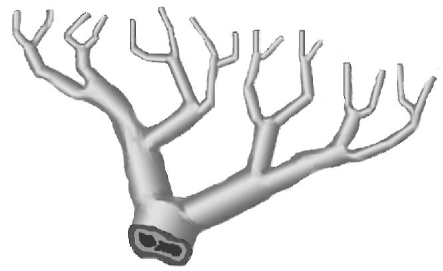
Figure 1: Thirty branches of capillaries.

The dilation of each capillary is caused by the fluctuation of the firing number associated with it, i.e., if more than $N_{firing}$ neurons that this capillary supplies are firing, this capillary is going to be dilated after $\Delta t$ time steps and this dilation will last $d_{c}$ time steps. In a first set of simulations, all the synapse strengths are uniformly distributed between -1 and 1, the blood flow turned out to be highly incompatible, since the blood flow difference fluctuated between 3000 and 8000 $\mu m^{3}/ms$ (also see Fig.  2).

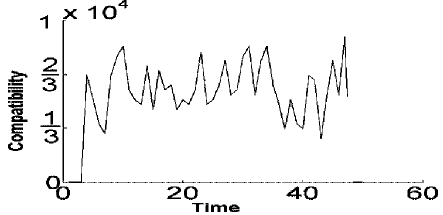
Figure 2: Compatibility for the model with synaptic weights uniformly distributed between -1 and 1. The blood flow is not compatible.

In the second simulation, we manually set these strengths to be uniformly distributed between $2\mu-1$ and 1, i.e., the mean value of them is $\mu$, which we call local-shift. Initially, the neuron states are set according to the rule that 1/4 of the neurons are firing. The simulation results are shown in Fig. 3. We found that this initialization had no effect on the behavior of the system; neurons will reach their resting state, which is determined by $\mu$. Over a certain short time period (from T=101 to T=105 in this simulation), we increased the Gaussian noise in this area so this positive input forces a number of neurons to fire. Then the neurons’ state will be changed to ’excitatory’, and at the same time the high level of neuron firing will trigger the dilation of capillaries. The results imply that this temporary external noise triggers the ’excitatory’ state and that a local shift $\mu$ helps the maintenance of this state until the next inhibitory signal arrives. This quick change from ’resting’ to ’excitatory’ makes the incompatible time really short, so in this way, these coupled networks function well.

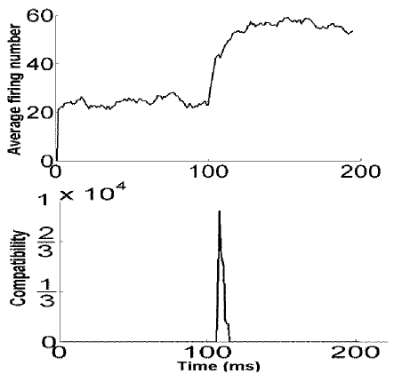
Figure 3: Average firing number per branch (top): We calculated the firing number associated with each branch of capillary, evaluated the mean value and plotted in this figure. Compatibility (bottom): The incompatible time is really short because the neurons quickly change from ’resting’ to ’excitatory’.

Based on these results, we can make a few hypotheses about the neurovascular coupling in the brain. The first hypothesis is that the local synapses are likely to have positive strengths. This enables the cluster of neurons to maintain either the ’excitatory’ state or the ’resting’ state, and external signals cause the switch between these two states. From simulations we can see that this switch is fast, although the capillaries react with time delay, the incompatible time is so short that it can be ignored. Secondly, since the local shift of the synapse weights is so tiny, we could assume that this is associated with the neuronal communication. The communication between neurons could slightly change the strength of synapses connected them, and this change is on the same time scale as the dilation of the capillaries. Because the neuron state is determined by this local-shift, changing of strength could result in changing of state, and at the same time balance the blood flow.

It is now believed that glial cells (astrocytes) also have their own network (via Calcium waves) in the brain and that this network also plays a distinct role in information processing. Calcium waves can both propagate among networks of astrocytes globally and send specific Calcium signals to a small number of nearby astrocytes [14]. In other words, glial signalling also has its preferred routes. Communication between glial cells and neurons is bidirectional and complex. Astrocytes are very sensitive to the level of neuronal activity because of their position and their sensitivity to activity-dependent changes in the chemical environment shared by neurons and astrocytes [7, 15]. Astrocytic Calcium waves can be triggered by synaptically-released neurotransmitters and in addition the frequency of these Calcium oscillations can change according to the level of synaptic activity [16]. It is observed that activated astrocytes can control the synaptic transmission by regulating the release of neurotransmitter from the nerve terminal. This regulation can be either excitatory (by secreting the same neurotransmitter) or inhibitory (by absorbing the neurotransmitter). If regulation of synaptic activities is the short-term effect of astrocytes, they can also change long-term synaptic strengths by releasing signalling molecules that cause the axon to increase or decrease the amount of neurotransmitter [14]. To sum up briefly, it is now possible to model the neuron-to-astrocyte coupling because many recent experiments confirm the signalling pathways among these two types of networks. Neurons communicate with neurons while astrocytes ’listen to’ the neuronal communication. Basing upon what they ’hear’, astrocytes regulate neuronal activities and communicate with other astrocytes. In order to quantify these regulations, we will define rules dependent on several parameters and then simulate this model.

The neuronal network contains 900 neurons, each of which has either a ’1’ state (firing) or a ’0’ state (resting). There are 3600 astrocytes in the glial network. In order to simplify, we suppose these astrocytes are in a $60\times 60$ matrix $G$. The state of an astrocyte is $g_{i,j}$ and it could be zero or a positive number. These 3600 astrocytes have their own connections, too. Because Calcium signals are more likely to propagate among nearby astrocytes, we assume here that the connection between astrocyte $(i1,j1)$ and $(i2,j2)$ is given by probability $\rho$, which is inversely proportional to the distance between them ($\sqrt{(i1-i2)^{2}+(j1-j2)^{2}}$). Since these connections are in fact invisible Calcium signal pathways, we did not give them weights. Unlike electrical signals travelling between neurons, Calcium signals need more time to travel from one astrocyte to another, and we set this time delay proportional to the distance.

The coupling between the neuronal network and the glial network is complicated. We will assume that each neuron has four astrocytes nearby which are all sensitive to this neuron’s activity. At the same time, because in the brain a single astrocyte can cover a large number of synapses [9], in our model we allocate to each astrocyte 1/4 of all the afferent synapses of this neuron, so that four nearby astrocytes can cover all afferent synapses without overlapping. Astrocytes can sense the spike frequency along each synapse, regulate the release of neurotransmitters, and change the synaptic strength. A simplified illustration of the position of neurons and astrocytes can be found in Fig. 4. There are two factors which affect the state of an astrocyte. The first one is high frequency effective spikes along synapses that this astrocyte is sensing, and ’effective’ means either a positive spike making the target neuron fire or a negative spike making it rest. The second factor is the Calcium signals from other astrocytes, and this part can accumulate as well. If the input signal of an astrocyte exceeds a certain threshold , this astrocyte will become active, which means that the state of the astrocyte is nonzero. Since activated astrocytes can have different levels of activation, we define that when activated, an astrocyte’s state equals its input.

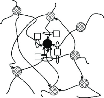
Figure 4: The position of one neuron (black circle) and 4 nearby astrocytes (rectangles). To make it clear, only afferent synapses from other neurons (shadowed circle) are drawn. The arms of astrocytes (ellipses) surround some synapses to sense and regulate their activities.

As mentioned previously, activated astrocytes can regulate the release of neurotransmitters over short periods of time ($<50s$) [17], in other words; they can change the input signal of the nearby neuron within a few seconds. Because the conditions for excitation and inhibition are unknown, we will make the following assumptions. The neuron’s input will be increased by an activated astrocyte proportionally to its state, but if this astrocyte was over-activated (its state exceeded a certain value), it would inhibit the input of the neuron. In the brain this local rule may be more complicated, and we believe that this interaction between neurons and astrocytes is crucial to short-term memory and information processing.

Meanwhile, as a long-term effect, astrocytes can also monitor the synaptic activities and gradually modify the strengths of synaptic connections (efficacies). This mechanism is also called adapting synapses, and has been studied before [18]. Because our model is based on discrete time, the update rule of synaptic strengths is quite simple. For a positive synapse, we look back 20 time steps and calculate the spike frequency of this synapse and the firing frequency of the neuron. If both of the two frequencies are high and correlated, in other words, the high firing rate is triggered by episodes of high synaptic activity through this connection (we call it excitation success), we will make this connection stronger. On the other hand, if this synapse is negative, it will be enhanced if the spike frequency is high but the neuron is firing at a low rate (inhibition success). The strength can also be weakened if high spike frequency along a positive synapse does not cause high firing rate (excitation failure) or high spike frequency along a negative synapse does not cause low firing rate (inhibition failure). Although due to limitations of computing time, our simulating time can not be long enough to represent the gradual changing of efficacy; we still include this procedure in our program. We believe that the distribution of synaptic strengths heavily affects the emergent behavior of neuron-to-astrocyte coupling, so it is crucial in understanding the brain function, especially long-term memory and learning [19, 20].

$$n_{p}(t+1)=\frac{1}{2}sgn(\sum_{q=1}^{900}T_{qp}(t)n_{q}(t)+\sum_{r=1}^{4}g_{4p+r}(t)-\varphi_{p}(t)+\eta)+\frac{1}{2}$$ (2)

Finally, we will explain the time resolution of this model. Based on the absolute refractory period of neurons, we suppose that each time step in our simulation equals 1 ms in the real brain. Since neurons can not be firing at two consecutive time steps, the maximum firing frequency is 500 Hz. At each time step, we loop over all astrocytes, all neurons and all synapses and change their states according to the rules we have defined above. The update rule for a neuron can be found in Eq.(2), in which $T_{qp}(t)$ represents the time-dependent strength, $\sum_{r=1}^{4}g_{4p+r}(t)$ means contributions from astrocytes and $\varphi_{p}(t)$ and $\eta$ are the threshold and noise, respectively.

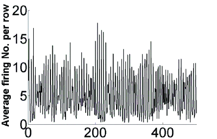
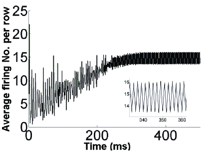
Figure 5: Top figure: Average number of firing neurons in each row in our simulation of pure neurons. Bottom figure: average number of firing neurons in each row in our simulation of neuron-to-astrocyte coupling.

Our results (Fig.5) imply that in the pure neuronal network, neuronal activity was quite random within the whole 500 time steps. While in the simulation with both neurons and astrocytes, it is obvious that there was an attractor in the neuronal network, after T=300, the neuronal network just oscillated between two states. If we compare the two figures concerning average firing number in Fig. 5, it is easy to find out that the firing frequency of neurons in the coupled network is much higher than that in the pure neuronal network. According to our simulations, on average 17 percent of all neurons were firing in the pure neuronal network while in the coupled network it was 39.2 percent. This is mainly because astrocytes changed the strengths of many synapses. At the same time, activated astrocytes enhancing the afferent spikes play a small part in this as well.

We have shown that a modification of the synapse strengths can allow the neuronal firing and the cerebrovascular flow to be compatible on a meso-scale. With astrocyte signalling added, limit cycles exist in the coupled networks. This is a first step towards a better understanding of the coupling of neuronal, astrocyte and cerebrovascular networks in the brain. This coupling is essential in any modern description of the brain, and has to be investigated using methods of complex systems. They will ultimately show the right scale for the models, and whether critical phenomena exist.

References

- [1] P. G. Haydon, Nat. Neurosci. 2, 185 (March 2001).
- [2] S. J. Mulligan and B. A. MacVicar, Nature 431, 195 (2004).
- [3] C. Iadecola, Nat. Neurosci. 5, 347 (May 2004).
- [4] L. F. Abbott and W. G. Regehr, Nature 431, 796 (2004).
- [5] D. B. Chklovskii, B. W. Mel and K. Svoboda, Nature 431, 782 (2004).
- [6] G. A. Cowan, Working Papers from Santa Fe Institute (1988).
- [7] R. D. Fields and B. Stevens-Graham, Science 298, 556 (2002).
- [8] K. Braet, L. Cabooter, K. Paemeleire and L. Leybaert, Biol. Cell 96, 79 (2004).
- [9] G. Perea and A. Araque, J. Physiol. - Paris 96, 199 (2002).
- [10] J. J. Hopfield, Proc. Natl. Acad. Sci. USA 79, 2554 (1982).
- [11] J. M. Casado, Phys. Rev. Lett. 91, 208102 (2004).
- [12] P. De Wilde, Neural Network Models (Springer-Verlag, 1997).
- [13] http://www.uoguelph.ca/ dstevens/teach/320/problems.htm.
- [14] R. D. Fields, Sci. Am. 54, (Apr 2004).
- [15] T. Fellin and G. Carmignoto, J. Physiol. 559, 1 (2004).
- [16] M. Zonta and G. Carmignoto, J. Physiol. - Paris 96, 193 (2002).
- [17] J. Kang, S. A. Goldman and M. Nedergaard, Nat. Neurosci. 1, 683 (1998).
- [18] D. W. Dong and J. J. Hopfield, Networks 3, 267 (1992).
- [19] A. Destexhe and E Marder, Nature 431, 789 (2004).
- [20] M. Tsodyks and C. Gilbert, Nature 431, 775 (2004).