A Tracer Driver for Versatile Dynamic Analyses of Constraint Logic Programs^,

Abstract

Programs with constraints are hard to debug. In this paper, we describe a general architecture to help develop new debugging tools for constraint programming. The possible tools are fed by a single general-purpose tracer. A tracer-driver is used to adapt the actual content of the trace, according to the needs of the tool. This enables the tools and the tracer to communicate in a client-server scheme. Each tool describes its needs of execution data thanks to event patterns. The tracer driver scrutinizes the execution according to these event patterns and sends only the data that are relevant to the connected tools. Experimental measures show that this approach leads to good performance in the context of constraint logic programming, where a large variety of tools exists and the trace is potentially huge.

1 Introduction

Program with constraints are especially hard to debug. The numerous constraints and variables involved make the state of the execution difficult to grasp. Moreover, the complexity of the filtering algorithms as well as the optimized propagation strategies lead to a tortuous execution. As a result, when a program gives incorrect answers, misses expected solutions, or has disappointing performances, the developer gets very little support from the current programming environment to improve the program. This issue is critical because it increases the expertise required to develop constraint programs.

Various work have addressed this critical issue. Most of them are based on dynamic analyses. During the execution, some data are collected in the execution so as to display some graphical views, compute some statistics and other abstraction of the execution behavior. Those data are then examined by the programmer to have a better understanding of the execution. For instance, a display of the search-tree helps to know how the search heuristics behaves [8]. Adding some visual clues about the domain propagation helps to see when the constraint propagation seems inefficient [2]. A more detailed view of the propagation in specific nodes of the search-tree gives a good insight to find out redundant constraints or select different filtering algorithms. A common observation is that there is no ultimate tool, that would meet all the debugging needs. There exists a large variety of complementary tools, from coarse-grained abstraction of the whole execution to very detailed views of small subparts, and even application-specific displays.

The existing tools imply a dedicated instrumentation of the execution, or a dedicated annotation of the traced program, to collect the data they need. Those instrumentations are often hard to make and strongly limit the use and the development of the tools. In this paper, we present a generic approach where the possible tools are fed by a single general-purpose tracer. A tracer-driver is used to adapt the actual content of the trace, according to the needs of the tool. This enables the tools and the tracer to communicate in a client-server scheme. Each tool describes its needs of execution data thanks to event patterns. The tracer driver scrutinizes the execution according to these event patterns and sends only the data that are relevant to the connected tools. A synchronisation mechanism allows the tools to retrieve on demand more data about a given execution event. Our experiments show that this architecture drastically reduces the amount of trace data and significantly improves the performance.

Another description of the tracer driver focuses on the architecture and implementation details, which are independent of the traced programming language [12]. This paper focuses on the use of the tracer driver for CLP. Its main contribution is an in-depth description of the good performance of the approach, and especially of what is gained in the trace communication and generation.

The paper is organized as follows. Section 2 briefly presents the features of the tracer driver. Section 3 describes the event patterns used to describe the needs of the tools. Section 4 lists the requests that an analyzer can send to our tracer and how they are taken into account. Section 5 justifies the format used to communicate the trace. Section 6 assesses the performance of the scheme. Section 7 discusses related work.

2 Overview of the tracer driver

This Section presents an overview of the tracer driver architecture and, in particular, the interactions it enables between a tracer and analyzers. An analyzer is any tool that processes the trace. The tracer and the analyzers are run at the same time. Both synchronous and asynchronous interactions are necessary between the tracer and the analyzers. On the one hand, if analyzers need to get complements of information at some events, it is important that the execution does not proceed until the analyzers have decided so. On the other hand, if the analyzers only want to collect information there is no need to block the execution.

An execution trace is a sequence of observed execution events that have attributes. The analyzers specify the events to be observed by means of event patterns. An event pattern is a condition on the attributes of an event (see details in Sect. 3). The tracer driver manages a base of active event patterns. Each execution event is checked against the set of active patterns. An event matches an event pattern if and only if the pattern condition is satisfied by the attributes of this event.

An asynchronous pattern specifies that, at matching trace events, some trace data are to be sent to analyzers without freezing the execution. A synchronous pattern specifies that, at matching trace events, some trace data are to be sent to analyzers. The execution is frozen until the analyzers order the execution to resume. An event handler is a procedure defined in an analyzer, that is called when a matching event is encountered.

The architecture enables the management of several active patterns. Each pattern is identified by a label. A given execution event may match several patterns. When sending the trace data to the analyzers the list of (labels of) matched patterns is added to the trace. Then, the analyzer mediator calls specific handlers for each matched pattern and dispatches relevant trace data to them. If at least one matched pattern is synchronous, the analyzer mediator waits for every synchronous handler to finish before sending the resuming command to the tracer driver. From the point of view of a given event handler, the activation of other handlers on the same execution event is transparent. Further details about this architecture can be found in Langevine and Ducassé [12].

This article emphasizes more the tracer driver than the analyzer mediator. On the one hand, the design and implementation of the tracer driver is critical with respect to response time. Indeed it is called at each event and executions of several millions of events (see Sect. 6) are very common. Every overhead, even the tiniest, is therefore critical. On the other hand, the implementation of the analyzer mediator is easier and much less critical because it is called only on matching events.

3 Event patterns

As already mentioned, an event pattern is a condition on the attributes of events. It consists of a first order formula combining elementary conditions on the attributes. This section summarizes the format of the trace events, specifies the format of the event patterns and gives examples of patterns.

3.1 Trace events

The actual format of the trace events has no influence on the tracer driver mechanisms. The important issue is that events have attributes and that some attributes are specific to the type of events. The trace format that we use is dedicated to constraint programming over finite domains, formally defined in [13].

There are 15 possible event types in the tracer we use (choice-point, failure, solution, back-to, new-variable, new-constraint, post, awake, reduce, suspend, entail, reject, schedule, begin-exec, end-exec). Each event has common and specific attributes. The common attributes are: the event type (called “port”), a chronological event number, the depth of the current node in the search-tree, the solver state (domains, constraint store and propagation queue), and the user time spent since the beginning of the execution. The specific attributes depend on the port. For instance, a domain reduction event carries data about the reduced variable (e.g. identifier and name), the reducing constraint (e.g. external representation) and the removed values.

1 newVariable   v1=[0-268435455]
2 newVariable   v2=[0-268435455]
3 newConstraint c1 fd_element([v1,[2,5,7],v2])
4 reduce c1 v1=[1,2,3] W=[0,4-268435455]
5 reduce c1 v2=[2,5,7] W=[0-1,3-4,6,8-268435455]
6 suspend c1

Figure 1: A portion of trace for fd_element(I,[2,5,7],A), (A#=I;A#=2)

Fig. 1 presents the beginning of a trace of a toy program in order to illustrate the events described above. This program specifies that A is a finite domain variable which is in $\{2,5,7\}$ and I is the index of the value of A in this list; moreover A is either equal to I or equal to 2. The second alternative is the only feasible one. The trace can be read as follows. The first two events are related to the introduction of two variables v$1$ and v$2$, corresponding respectively to I and A. In Gnu-Prolog, variables are always created with the maximum domain (from 0 to 268.435.455). Then the first constraint is created: fd_element (event #3). This constraint makes two domain reductions (events #4 and #5): the domain of the first variable (I) becomes $\{1,2,3\}$ and the domain of A becomes $\{2,5,7\}$. After these reductions, the constraint is suspended (event #6). The execution continues and finds the solution A=2,I=1 through 32 other events not shown here.

3.2 Patterns

pattern	::=	label: when evt_pattern  op_synchro  action_list
op_synchro	::=	do  |  do_synchro
action_list	::=	action  ,  action_list  |  action
action	::=	current(list_of_attributes)  |  call(procedure)
evt_pattern	::=	evt_pattern  or  evt_pattern (1)
		| evt_pattern  and  evt_pattern (2)
		| not  evt_pattern (3)
		| ( evt_pattern ) (4)
		| condition (5)
condition	::=	attribute  op2  value  |  op1(attribute)  |   true
op2	::=	< | > | = | $\backslash$= | >= | =< | in | notin | contains | notcontains
op1	::=	isNamed
value	::=	integer | domain | string
attribute	::=	vident | vname | cident | cname | port | vdom | delta | chrono
		| depth | time | stage | node

Figure 2: Grammar of event patterns

We use patterns similar to the path rules of Bruegge and Hibbard [3]. Fig. 2 presents the grammar of patterns. A pattern contains four parts: a label, an event pattern, a synchronization operator and a list of actions. An event pattern is a composition of elementary conditions using logical conjunction, disjunction and negation. A synchronization operator tells whether the pattern is asynchronous (do) or synchronous (do_synchro). An action specifies either to ask the tracer driver to collect attribute values (current(list_of_attributes)), or to ask the analyzer to call a procedure call(procedure). Such a procedure is written in a language that the analyzer can execute. This language is independent of the tracer driver. An elementary condition concerns an attribute of the current event.

There are several kinds of attributes. Each kind has a specific set of operators to build elementary conditions. For example, most of the common attributes are integer (chrono, depth, node label). Classical operators can be used with those attributes: equality , disequality ($\neq$), inequalities ($<$, $\leq$, $>$ and $\geq$). The port attribute has a set of 15 possible values. The following operators can be used with the port attribute: equality and disequality ($=$ and $\neq$) and two set operators, in and notin. Constraint solvers manipulate a lot of constraints and variables. Often, a trace analysis is only interested in a small subset of them. Operators in and notin, applied to identifiers of entities or name of the variables, can specify such subsets. Operators contains and notcontains are used to express conditions on domains.

3.3 Examples of patterns

visu_tree:  when port in [choicePoint,solution,failure,backTo]
    do current(port=P and node=N and time=T),
       call buildTree(P,N,T)
new_cstr:   when port=newConstraint and stage=’labeling’
    do current(cstrRep=Constraint),
       call recordDecision(Constraint)
visu_prop1: when port=reduce do current(vident=V and cident=C),
       call countReduce(V,C)
visu_prop2: when port=awake do current(cident=C),
       call countAwake(C)
synchronize: when port in [solution,failure]
    dosynchro refreshViewer(void)

Figure 3: Examples of patterns for visualization and monitoring

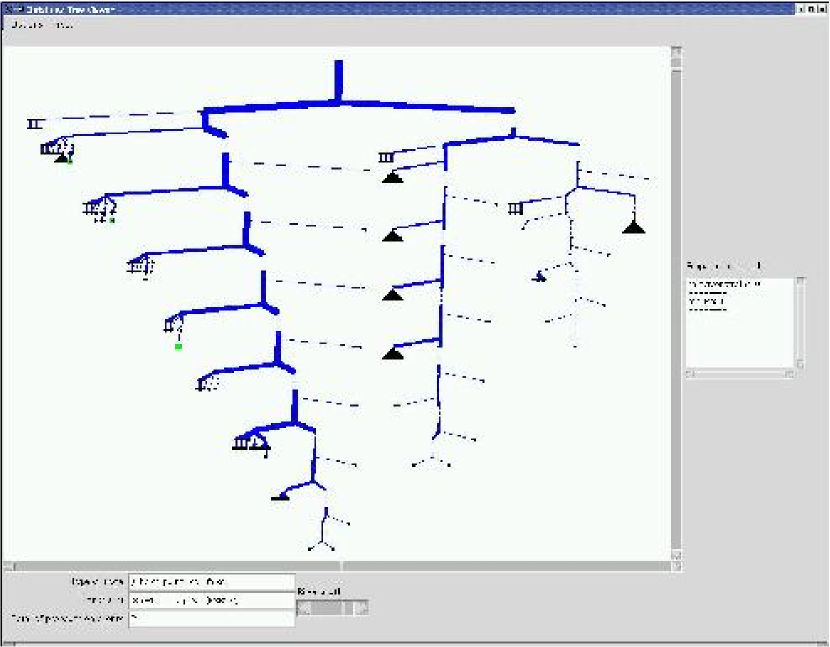
Figure 4: A display based on the patterns of Fig. 3.

Fig. 3 presents five patterns that can be activated in parallel. These patterns aim at producing a more or less precise view of the search-tree. Following the user’s parametrization, some of these patterns can be disabled, so as to tune the trace volume. The first pattern (visu_tree) simply asks for a trace of the search-tree events: declaration of choice-points, of leafs and of backtrackings. This is enough to compute the structure of the search-tree. The second pattern (new_cstr) adds to the trace the posting of every decision constraint (a constraint that is posted by the labeling procedure). It allows the edges of the search-tree to be labeled with the decision constraints they represent. Those two patterns gives the basic data for the search-tree viewer: they are always enabled when the viewer is running.

The following two patterns are added when more detailed data about the nodes are needed. (visu_prop1) asks for the trace of every domain reduction, with the identifiers of the reduced variable and the reducing constraint. (visu_prop2) is interested in every constraint awakening, with the identifier of the awakened constraint. The various combinations of these two patterns allow the computation of statistics about the number of constraint reduction, the number of awakening or the proportion of useful awakenings (awakenings followed by at least one domain reduction) in each node. Such statistics can be used to add visual clues on the search tree. For instance, the size of the nodes or the width of the edges can depend on one of those indicators.

The last pattern synchronizes the display with the execution. The execution is often running much faster than its visualization. This issue can be adressed by such a synchronization mechanism. Fig. 4 shows a screenshot of the viewer using those five patterns according to the user needs. In this configuration, the width of the row depends on the total number of propagation events (domain reductions and constraint awakenings) occurring in the subtree.

4 Analyzer mediator

The analyzer mediator processes the trace: it specifies to the tracer driver what events are needed and may execute specific actions for each type of relevant events. The analyzer can supervise several analyses at a time. Each analysis has its own purpose and uses specific pieces of trace data. The independence of the concurrent analyses is ensured by the mediator that centralizes the communication with the tracer driver and dispatches the trace data to the ongoing analyses.

The requests that an analyzer can send to the tracer driver are of three kinds. Firstly, the analyzer can ask for additional data about the current event. Secondly, the analyzer can modify the event patterns to be checked by the tracer driver (the active patterns). Thirdly, the analyzer can notify the end of a synchronous session.

Primitive current specifies a list of event attributes to retrieve in the current execution event. The tracer retrieves the requested pieces of data and sends them to the mediator. reset deletes all the active event patterns and their labels.  Primitive remove deletes the active patterns whose labels are specified in the parameter.  Primitive add inserts, in the active patterns, the event patterns specified in the parameter, following the grammar described in Figure 2.  Primitive go notifies the tracer driver that a synchronous session is finished. The traced execution will be resumed.

step :-
  reset,
  add([step:when true
     dosynchro call(tracer_toplevel)]),
  go.
skip_reductions :-
  current(cstr = CId and port = P),
  reset,
  (  P == awake
  -> add([sr:when cstr = CId and port
    in [suspend,reject,entail] dosynchro call(tracer_toplevel)]),
  ;  add([step:when true dosynchro call(tracer_toplevel)])),
  go.

Figure 5: Implementation of two tracing commands

Fig. 5 illustrates the use of the primitives to implement two tracing commands. Command step enables to go to the very next event. It simply resets all patterns and adds one pattern which will match any event (the associated condition is always true). This pattern calls, in a synchronous way, the tracer toplevel. Therefore, the tracer will call the toplevel at each event, and the toplevel will be synchronized with the execution: the user will be able to investigate the current state of the execution before resuming the execution. Command skip_reductions enables to skip the details of variable domain reductions when encountering the awakening of a constraint. It first retrieves the current port, if it is awake it asks to go to the suspension of this constraint: the possible domain reductions are skipped. There, the user will, for example, be able to check the value of the domains after all the reductions. If the command is called on an event of other type it simply acts as step, so the tracer will stop on the very next event.

5 A Suitable Trace Format

An execution can generate several millions of execution events per second. Large pieces of data can be attached to each event. The tracer driver filters this trace according to the needs of the analyzers. In this section, we study the properties of a good format for execution traces to be sent from the tracer to the analyzers. We consider several issues: the ability of the format to represent partial (filtered) trace, the volume of the encoded trace, and processing easiness.

<reduce time="1045" vident="v13" />

<reduce cident="c12" vident="v13" />

<reduce chrono="1145697" time="1045" cident="c12" vident="v13"
        cexternal="greaterEq(v13,v19)">
  <delta vident="v13"><range from="0" to="21" /></delta>
  <update vident="v13" type="min" />
</reduce>

Figure 6: Three possible trace of the same event

The tracer can access a large amount of data at each execution event. Among those data, only a small subpart is in general needed for a specific debugging tools. Therefore, the tracer driver only communicates a small subset of the attributes and a part of the current state. The concrete format has then to enable partial traces to be represented, without losing the structure of the trace. An instance of trace can thus be seen as an excerpt of the exhaustive trace. The OADymPPaC project addressed this issue by designing an XML format where most of the elements and attributes (in the sense of XML) are optional [14]. For instance, Fig. 6 presents three possible versions of the very same execution event, a reduction of a domain. The first version only displays few basic attributes of the event: the user-time when the event occurs and the identifier of the variable. The second version hides the user-time but displays also the identifier of the reducing constraint, as well as some data about the values that have just been removed. The third one is more complete: it displays the full set of removed values, the external representation of the acting constraint and the chronological number of the event. From an XML point-of-view, they are three different excerpts of the same document. Of course, the exhaustive document is never produced: the tracer driver only fills the parts that are relevant according to the active patterns.

Since XML is a standard and widely-used format, an interested developer can choose among dozens of libraries to parse the trace data. Moreover, XML answers the needs of trace structuring thanks to the notion of attributes and nested elements. An event is an XML element that contains all its attached data. It is worth noticing that there exists a standard binary representation of XML: a table of symbols copes with the verbosity of XML and speeds up the parsing of the trace [7].

6 Experimental Results

This section assesses the performances of the tracer driver and its effects on the cost of the trace generation and communication. It shows several things. The overhead of the core tracer mechanisms is small. The core tracer can thus be permanently activated. The tracer driver overhead is acceptable and can be predicted. There is no overhead for parallel search of patterns. The tracer driver approach that we propose is more efficient than sending over a default trace, even to construct sophisticated graphical views. Answering queries is orders of magnitude more efficient than displaying traces. There is no need to a priori restrict the trace information. The performance of our tool is comparable to the state-of-the-practice while being more powerful and generic.

6.1 Methodology of the Experiments

When tracing a program, some time is spent in the program execution ($T_{prog}$), some time is spent in the core mechanisms of the tracer ($\Delta_{tracer}$), some time is spent in the tracer driver ($\Delta_{driver}$), some time is spent generating the requested trace and sending it to the analysis process ($\Delta_{gcom}$), some time is spent in the analyses ($\Delta_{ana}$). Hence, if we call $T$ the execution time of a traced and analysed program, we approximatively have: $T\simeq T_{prog}+\Delta_{tracer}+\Delta_{driver}+\Delta_{gcom}+\Delta_{ana}$.

The mediator is a simple switch. The time taken by its execution is negligible compared to the time taken by the simplest analysis, namely the display of trace information. Trace analysis takes a time which vary considerably according to the nature of the analysis. The focus of this article is not to discuss which analyses can be achieved in reasonable time but to show that a flexible analysis environment can be offered at a low overhead. Therefore, in the following measurements $\Delta_{ana}=0$.

The experiments have been run on a PC, with a 2.4 GHz Pentium iv, 512 Kb of cache, 1 GB of RAM, running under the GNU/Linux 2.4.18 operating system. The stable release (1.2.16) of GNU-Prolog has been used. The tracer is an instrumentation of the source code of this very same version and has been compiled in the same conditions by gcc-2.95.4. The execution times have been measured with the GNU-Prolog profiling predicates whose accuracy is 1 ms. The measured executions consist of a batch of executions such that each measured time is at least 20 seconds. The measured time is the sum of system and user times. Each experimental time given below is the average time of a series of ten measurements. In each series, the maximal relative deviation was smaller than 1 %.

6.2 Benchmark programs

The 9 benchmark programs are listed in Table 6.2, sorted by increasing number of trace events. Magic(100), square(4), golomb(8) and golfer(5,4,4) are part of CSPLib, a benchmark library for constraints by Gent and Walsh [9]. The golomb(8) program is executed with two strategies which exhibit very different response times. Those four programs have been chosen for their significant execution time and for the variety of constraints they involve. Four other programs have been added to cover more specific aspects of the solver mechanisms: Pascal Van Hentenryck’s bridge problem (version of [4]); two instances of the $n$-queens problem; and “propag”, the proof of infeasibility of $1\leq x,y\leq 70000000\wedge x<y\wedge y<x$.

Program	evts ($10^{6}$)	Trace Size (Gb)	$T_{prog}$ (ns)	$\varepsilon$	$R_{tr.}$	Dev. for $T_{x}$
bridge	0.2	0.1	14	72	1.21	$\leq 0.4\%$
queens(256)	0.8	1.5	173	210	1.14	$\leq 0.2\%$
magic(100)	3.2	1.4	215	66	1.03	$\leq 0.2\%$
square(24)	4.2	20.8	372	88	1.05	$\leq 0.6\%$
golombF	15.5	3.4	7,201	464	1.01	$\leq 0.4\%$
golomb	38.4	7.9	1,721	45	1.00	$\leq 0.5\%$
golfer(5,4,4)	61.0	>30	3,255	53	1.05	$\leq 0.7\%$
propag	280.0	>30	3,813	14	1.28	$\leq 1.0\%$
queens(14)	394.5	>30	17,060	43	1.08	$\leq 0.4\%$

Table 1: Benchmark Programs and tracer overhead

The benchmark programs have executions large enough for the measurements to be meaningful. They range from 200,000 events to about 400 millions events. Furthermore, they represent a wide range of CLP(FD) programs.

The third column gives the size of the traces of the benchmarked programs for the default trace model. All executions but the smallest one exhibit more than a gigabyte, for executions sometimes less than a second. It is therefore not conceivable to systematically generate such an amount of information. As a matter of fact measuring these size took us hours and, in the last three cases, exhausted our patience! Note that the size of the trace is not strictly proportional to the number of events because the attributes collected at each type of events are different. For example, for domain reductions, several attributes about variables, constraints and domains are collected while other types of events simply collect the name of the corresponding contraint.

The fourth column gives $T_{prog}$, the execution time in $ms$ of the program simply run by GNU-Prolog. The fifth column shows the average time of execution per event $\varepsilon=\frac{T_{prog}}{\mathrm{Nb.\ evt.}}$. It is between 14 ns and 464 ns per event. For most of the suite $\varepsilon$ is around 50ns. The three remarkable exceptions are propag ($\varepsilon=14$ ns), queens(256) ($\varepsilon=210$ ns) and golombF ($\varepsilon=464$ ns). The low $\varepsilon$ is due to the efficiency of the propagation stage for the constraints involved in this computation. The large $\varepsilon$s are due to a lower proportion of “fine-grained” events.

Core tracer mechanisms can be permanently activated

Table 6.2 also gives the results of the measurements of the overhead of the core tracer mechanisms. Those results have already been discussed in [13]. For all the measured executions $R_{tracer}$ is less than 30% in the worst case, and less than 5% for five traced programs. That is are very positive. The core mechanisms of the tracer can be systematically activated. Users will hardly notice the overhead. Therefore, while developping programs, users can directly work in “traced” mode, they do not need to switch from untraced to traced environments. This is a great confort.

6.3 Tracer driver overhead

The measure of $T_{driver}\simeq T_{prog}\!+\!\Delta_{core\_trace}\!+\!\Delta_{driver}$ is the execution time of the program run by the tracer with the filtering procedure activated for generic patterns. Only the attributes necessary for the requested patterns are calculated at relevent events. In order for $\Delta_{gcom}$ to be zero, the patterns are designed such that no event matches them. One run is done per pattern. The patterns are listed in Figure 6.2. Pattern 1a is checked on few events and on one costly attribute only. Pattern 2a is checked on numerous events and on two costly attributes. Pattern 3a is checked on all events and on one cheap attribute. Pattern 4a is checked on all events and systematically on three attributes.

1a. when port=post and isNamed(cname) do current(port,chrono,cident).

2a. when port=reduce and (isNamed(vname) and isNamed(cname))

do current(port,chrono,cident).

3a. when chrono=0 do current(chrono).

4a. when depth=50000 or (chrono>=1 and node=9999999) do current(chrono,depth).

5a: patterns 1a, 2a, 3a and 4a activated in parallel.

Figure 7: Patterns used to measure the tracer driver overhead

Figure 8: Cost of the tracer driver mechanisms compared to $\mathbf{\varepsilon}$

Tracer driver overhead is acceptable

Figure 8 gives the results of the measurements of the overhead of the tracer driver for all the benchmark programs and for five patterns. The figure draws $R_{driver}=\frac{T_{driver}}{T_{prog}}$, compared to the average time per event ($\varepsilon$) for the 5 patterns. For all but one program, $R_{driver}$ is negligible for the very simple patterns and less than 3.5 for pattern 5a which is the combination of 4 patterns. For programs with a large $\varepsilon$, even searching for pattern 5a is negligible. In the worst case, an overhead of 8 is still acceptable.

No overhead for parallel search of patterns

When $n$ patterns are checked in parallel they already save $(n-1)T_{tracer}$ compared to the search in sequence which requires to executes $n$ times the program instead of one time. Figure 8 further shows that

$\Delta_{driver}^{1a}+\Delta_{driver}^{2a}+\Delta_{driver}^{3a}+\Delta_{driver}^{4a}>\Delta_{driver}^{(1|2|3|4)a}$.

As a matter of fact, the curve $\Sigma R=R_{1}+R_{2}+R_{3}+R_{4}-3$, that adds the overheads of the four separated patterns, is above the curve of $R^{5a}_{driver}$. This means that not only is there no overhead in the filtering mechanism induced by the parallel search, but there is even a minor gain.

Tracer driver overhead is predictable

The measured points of Figure 8 can be interpolated with curves of the form $R_{driver}=a+b/\varepsilon$. This means that the tracer and tracer driver overheads per event can be approximated to constants depending on the patterns and independant of the traced program.

6.4 Communication overhead

The measure of $T_{gcom}\simeq T_{core\_tracer}+\Delta_{driver}+\Delta_{gcom}$ is the execution time of the program run by the tracer. A new set of patterns are used so that some events match the patterns, the requested attributes of the matched events are generated and sent to a degenerated version of the mediator: a C-program that simply reads the trace data on its standard input. Due to lack of space we only show the result of program golomb(8) which has a median number of events and has a median $\varepsilon$.

1b. cstr: when port=post do current(chrono,cident,cinternal).

1b. tree: when port in [failure,backTo, choicePoint,solution] do current(chrono,node,port).

2b. newvar: when port=newVariable do current(chrono, vident, vname). 2b. dom: when port in [choicePoint,backTo,solution] 2b.do current(chrono,node,port,named_vars,full_dom).

3b. propag1: when port=reduce do current(chrono).

4b. propag2: when port=awake do current(chrono).

Figure 9: Event patterns used to assess the trace generation and the communication overhead

The patterns are listed in Figure 6.2. Pattern 1b, composed of two basic patterns, allows a “bare” search tree to be constructed, as shown by most debugging tools. Pattern 2b (two basic patterns) allows the display of 3D views of variable updates as shown in Figure 4. Pattern 3b and pattern 4b provide two different execution details to decorate search trees. Depending on the tool settings, three different visual clues can be displayed. One is shown in Figure 4.

Table 2: Cost of the trace generation and communication

Table 6.2 gives the results for the above patterns and some of their combinations. All combinations correspond to existing tools. For example, combining 1b with 3b or/and 4b allows a Christmas tree as shown in Figure 4 to be constructed with two different parameterizations. The 2^nd column gives the number of events which match the pattern. The 3^rd column gives the size of the resulting XML trace as it is sent to the tool. The 4^th column gives the elapsed time. The 5^th column gives the ratio $R_{driver}$, recomputed for each pattern. The 6^th column gives the ratio $R_{gcom}=\frac{T_{gcom}}{T_{prog}}$.

Filtered trace is more efficient and more accurate than default trace

The last line gives results for the default trace. The default trace contains twice as many events as the trace generated by pattern (1|2|3|4)b, but it contains more attributes than requested by the pattern; As a result, its size is ten times larger and its $R_{gcom}$ overhead is three times larger. As a consequence, the tracer driver approach that we propose is more efficient than sending over a default trace, even to construct sophisticated graphical views. The accuracy and the lower volume of the trace ease its post-processing by debugging tools.

Answering queries is more efficient than displaying traces

$R_{gcom}$ is always much larger that $R_{driver}$, from $2.6$ to $79.07$ in our exemple. Therefore, queries using patterns that drastically filter the trace have significantly better response time than queries that first display the trace before analysing it.

No need to a priori restrict the trace information

Many tracers limit a priori the trace information in order to reduce the volume of trace. This restricts the range of possible dynamic analyzes without preventing the big size and time overhead as shown above with the default trace: it lacks some important information while being huge.

With our approach, trace information which is not requested does not cost much, therefore our trace model can afford to be much richer. This enlarges the possibility of adding new dynamic analyses.

Performance are comparable to the state-of-the-practice

$R_{gcom}$ varies from 2.6 to 79.07. To give a comparison the Mercury tracer of Somogyi and Henderson [17] is regularly used by Mercury developers. For executions of size equivalent to those of our measurements, the Mercury tracer overhead has been measured from 2 to 15, with an average of 7 [11]. Hence the ratios for patterns 1b, 2b and 1|2b are quite similar to the state-of-the-practice debuggers. The other patterns show an overhead that can discourage interactive usage. However, these patterns are more thought of for monitoring than debugging when the interaction does not have to be done in real time. Note, furthermore, that for the measured programs, the absolute response time is still on the range of two minutes for the worst case. When debugging, this is still acceptable.

Our approach allows therefore to have the tracer present but idle by default. When a problem is encountered, simple queries can be set to localize roughly the source of the problem. Then, more costly patterns can be activated on smaller parts of the program. This is pretty much like what experienced programmers do. The difference with our approach is that they do not have to change tools, neither to reset the parameterizations of the debugger.

7 Related Work

Kraut [3] implements a finite state machine to find sequences of execution events that satisfy some patterns (“path rules”). Several patterns are allowed and they can be enabled or disabled during the execution, using a labeling policy. Specified actions are triggered when a rule is satisfied but they are limited to some debugger primitives, such as a message display or a counter increasing. The trace analysis is necessarily synchronous and cannot benefit from the power of a complete programming language.

Reiss and Renieris [15] have an approach similar to ours. They also structure their dynamic analyses into three different modules: 1) extraction of trace, 2) compaction and filtering and 3) visualization. They provide a number of interesting compaction functions which should be integrated in a further version of our system. They, however, first dump the whole trace information in files before any filtering is processed. With our tracer driver filtering is done on the fly, and section 6 has shown that this is much more efficient than first storing in files.

Coca [5] and Opium [6] provide a trace query mechanism, respectively for C and Prolog. This mechanism is synchronous and does not allow concurrent analyses. It can be easily emulated with our tracer driver and an analyzer mediator written in Prolog.

UFO [1] offers a powerful language to specify patterns and monitors. The patterns can involve several events, not necessarily consecutive. In our framework, the monitors have to be implemented in the analyzer with a general programming language. A further extension should allow at least to implement monitors in the trace driver to improve efficiency. UFO, however, does not allow the same flexibility as our tracer driver, and is heavier to use for interactive debugging.

A debugging library for Sicstus Prolog has been implemented by Hanák et al [10]. No performance results are available. Some tuning of the trace display is possible but the tracer is based on a complete storage of the trace and a postmortem investigation: this is impractical with real-sized executions. The lazy generation of the trace our tracer implements leads to the same kind of trace data in a more efficient and practical way.

Some debugging tools enable the user to interact with the execution states. User acts on the current state of the execution to drive the search-tree exploration (Oz Explorer [16]), to add new constraints on a partial solution (CLPGUI [8]), to recompute a former state (both). Those features are really helpful but go much beyond the scope of this paper. Our approach is complementary: it addresses the communication from the traced execution to the debugging tools.

8 Conclusion

In this paper we presented a tracer driver which allows both synchronous and asynchronous trace analysis in the same execution, fitting all the needs of the classical usages of a tracer into a single tool. We have defined an expressive language of event patterns where relevant events are described by first order formulæ involving most of the data the tracer can access. Specific primitives enable the retrieval of large pieces of data “on demand” and the adaptation of the event patterns to the evolving needs of the trace analyzer. Therefore, the produced trace is accurate: trace generation, trace communication and trace post-processing are speeded up. As shown by the experiments, this approach leads to good performance in the context of constraint logic programming, where a large variety of tools exists and the trace is potentially huge. The tracer driver provides a powerful front-end for complex debugging tools based on trace data.

This approach has been prototyped in GNU-Prolog and is currently under development within SICStus Prolog.

Acknowledgment

The authors thank Pierre Deransart and their OADymPPaC partners for fruitful discussions, as well as Guillaume Arnaud for his careful beta-testing of Codeine.

References

- [1] M. Auguston, C. Jeffery, and S. Underwood. A framework for automatic debugging. In W. Emmerich and D. Wile, editors, Proceedings fo the 17th International Conference on Automated Software Engineering (ASE’02), pages 217–222. IEEE Press, 2002.
- [2] C. Bracchi, C. Gefflot, and F. Paulin. Combining propagation information and search-tree visualization using OPL studio. In A. Kusalik, editor, Proceedings of WLPE’01, pages 27–39, Cyprus, Décembre 2001. Computer Research Repository cs.PL/0111040.
- [3] B. Bruegge and P. Hibbard. Generalized path expressions: A high-level debugging mechanism. The Journal of Systems and Software, 3:265–276, 1983. Elsevier.
- [4] D. Diaz. Gnu prolog, 2003. http://gprolog.sourceforge.net/.
- [5] M. Ducassé. Coca: An automated debugger for C. In Proceedings of the 21st International Conference on Software Engineering, pages 504–513. ACM Press, May 1999.
- [6] M. Ducassé. Opium: An extendable trace analyser for Prolog. The Journal of Logic programming, 39:177–223, 1999. A. Bossi and Y. Deville (eds).
- [7] Ericsson, IBM, Motorola, and Phone.com. WAP binary XML content format. Note, W3C, http://www.w3.org/TR/wbxml/, June 1999.
- [8] F. Fages. Clpgui: a generic graphical user interface for constraint logic programming over finite domains. In A. Tessier, editor, Proc. of the 12th Workshop on Logic Programming Environments (Wlpe’02). Computer Research Repository cs.SE/0207048, 2002.
- [9] I.P. Gent and T. Walsh. CSPLib: a benchmark library for constraints. Technical report, APES-09-1999, 1999. Available from http://www.csplib.org/.
- [10] David Hanák, Tamás Szeredi, and Péter Szeredi. Fdbg, the clp(fd) debugger library of sicstus prolog. In B. Demoen and V. Lifschitz, editors, Proc. of Iclp’04, 2004. Poster. LNCS 3132.
- [11] E. Jahier and M. Ducassé. Generic program monitoring by trace analysis. Theory and Practice of Logic Programming, 2(4-5):611–643, July-September 2002.
- [12] L. Langevine and M. Ducassé. A tracer driver for hybrid execution analyses. In AADEBUG’05. ACM Press, 2005.
- [13] L. Langevine, M. Ducassé, and P. Deransart. A propagation tracer for Gnu-Prolog: from formal definition to efficient implementation. In C. Palamidessi, editor, Proc. of the 19th Int. Conf. on Logic Programming. Springer, LNCS 2916, 2003.
- [14] Ludovic Langevine and the OADymPPaC Team. Gentra4cp: a generic trace format for constraint programming. In 21th Int. Conf. on Logic Programming, pages 433–434. Springer, 2005. Poster.
- [15] S.P. Reiss and M. Renieris. Encoding program executions. In M.-J. Harrold and W. Schäfer, editors, Proc. of the 23rd Int. Conf. on Software Engineering. IEEE Press, 2001.
- [16] C. Schulte. Oz explorer: a visual constraint programming tool. In L. Naish, editor, Proc. of the 14th Int. Conf. on Logic Programming, pages 286–300. MIT Press, 1997.
- [17] Z. Somogyi and F. Henderson. The implementation technology of the Mercury debugger. In Proc. of the 10th WLPE, volume 30(4). Elevier, ENTCS, 1999.