Extending Prolog with
Incomplete Fuzzy Information

Abstract

Incomplete information is a problem in many aspects of actual environments. Furthermore, in many sceneries the knowledge is not represented in a crisp way. It is common to find fuzzy concepts or problems with some level of uncertainty. There are not many practical systems which handle fuzziness and uncertainty and the few examples that we can find are used by a minority. To extend a popular system (which many programmers are using) with the ability of combining crisp and fuzzy knowledge representations seems to be an interesting issue.

Our first work (Fuzzy Prolog) was a language that models $\mathcal{B}([0,1])$-valued Fuzzy Logic. In the Borel algebra, $\mathcal{B}([0,1])$, truth value is represented using unions of intervals of real numbers. This work was more general in truth value representation and propagation than previous works.

An interpreter for this language using Constraint Logic Programming over Real numbers (CLP(${\cal R}$)) was implemented and is available in the Ciao system .

Now, we enhance our former approach by using default knowledge to represent incomplete information in Logic Programming. We also provide the implementation of this new framework. This new release of Fuzzy Prolog handles incomplete information, it has a complete semantics (the previous one was incomplete as Prolog) and moreover it is able to combine crisp and fuzzy logic in Prolog programs. Therefore, new Fuzzy Prolog is more expressive to represent real world.

Fuzzy Prolog inherited from Prolog its incompleteness. The incorporation of default reasoning to Fuzzy Prolog removes this problem and requires a richer semantics which we discuss.

Keywords

Incomplete knowledge, Fuzzy Prolog, Modeling Uncertainty, Fuzzy Logic Programming, Constraint Programming Application, Implementation of Fuzzy Prolog.

1 Introduction

World information is not represented in a crisp way. Its representation is imperfect, fuzzy, etc., so that the management of uncertainty is very important in knowledge representation. There are multiple frameworks for incorporating uncertainty in logic programming:

• fuzzy set theory [2, 35, 30],

• probability theory [6, 17, 20, 22, 23],

• multi-valued logic [5, 13, 14, 16, 18, 26],

• possibilistic logic [4, 33, 34]

In [18] a general framework was proposed that generalizes many of the previous approaches. At the same time an analogous theoretical framework was provided and a prototype for Prolog was implemented [31]. Basically, a rule is of the form $A\leftarrow B_{1},\ldots,B_{n}$, where the assignment $I$ of certainties is taken from a certainty lattice, to the $B_{i}$s. The certainty of $A$ is computed by taking the set of the certainties $I(B_{i})$ and then they are propagated using the function $F$ that is an aggregation operator. This is a very flexible approach and in [32, 9] practical examples in a Prolog framework are presented.

In this work we extend the approach of [9] with arbitrary assignments of default certainty values (non-uniform default assumptions). The usual semantics of logic programs can be obtained through a unique computation method, but using different assumptions in a uniform way to assign the same default truth-value to all the atoms. The most well known assumptions are:

• the Closed World Assumption (CWA), which asserts that any atom whose truth-value cannot be inferred from the facts and clauses of the program is supposed to be false (i.e. certainty $0$). It is used in stable models [7, 8] and well-founded semantics [19, 20, 22],

• the Open World Assumption (OWA), which asserts that any atom whose truth-value cannot be inferred from the facts and clauses of the program is supposed to be undefined or unknown (i.e. certainty in $[0,1]$). It is used in [18].

There are also some approaches [33, 34] where both assumptions can be combined and some atoms can be interpreted assuming CWA while others follows OWA. Anyway, what seems really interesting is not only to combine both assumptions but to generalize the use of a default value. The aim is working with incomplete information with more guarantees.

The rest of the paper is organized as follows. Section 2 introduces the Fuzzy Prolog language. A complete description of the new semantics of Fuzzy Prolog is provided in Section 3. Section 4 completes the details about the improved implementation using CLP(${\cal R}$) with the extension to handle default knowledge. Some illustrating examples are provided in section 5. Finally, we conclude and discuss some future work (Section 6).

2 Fuzzy Prolog

In this section we are going to summarize the main characteristics of the Fuzzy Prolog that we proposed in [9] and that is the basis of the work presented here. Fuzzy Prolog is more general than previous approaches to introduce fuzziness in Prolog in some respects:

1. A truth value will be a finite union of closed sub-intervals on $[0,1]$. This is represented by Borel algebra, $\mathcal{B}([0,1])$, while the algebra $\mathcal{E}([0,1])$ only considers intervals. An interval is a special case of the union of one element, and a unique truth value is a particular case of having an interval with only one element.

2. A truth value will be propagated through the rules by means of an aggregation operator. The definition of aggregation operator is general in the sense that it subsumes conjunctive operators (triangular norms [15] like min, prod, etc.), disjunctive operators [28](triangular co-norms, like max, sum, etc.), average operators (like arithmetic average, quasi-linear average, etc) and hybrid operators (combinations of the above operators [25]).

3. The declarative and procedural semantics for Fuzzy Logic programs are given and their equivalence is proven.

4. An implementation of the proposed language is presented. A fuzzy program is a finite set of

   • fuzzy facts ($A\leftarrow v$, where $A$ is an atom and $v$, a truth value, is an element in $\mathcal{B}([0,1])$ expressed as constraints over the domain $[0,1]$), and

   • fuzzy clauses ($A\leftarrow_{F}B_{1},\ldots,B_{n}$, where $A,B_{1},\ldots,B_{n}$ are atoms, and $F$ is an interval-aggregation operator, which induces a union-aggregation, as by Definition 2.2, $\mathcal{F}$ of truth values in $\mathcal{B}([0,1])$ represented as constraints over the domain $[0,1]$).

   We obtain information from the program through fuzzy queries or fuzzy goals ($v\leftarrow A~{}?$ where $A$ is an atom, and $v$ is a variable, possibly instantiated, that represents a truth value in $\mathcal{B}([0,1])$).

Programs are defined as usual but handling truth values in $\mathcal{B}([0,1])$ (the Borel algebra over the real interval $[0,1]$ that deals with unions of intervals) represented as constraints. We refer, for example, to expressions as: $(v\geq 0.5~{}\wedge~{}v\leq 0.7)~{}\vee~{}(v\geq 0.8~{}\wedge~{}v\leq 0.9)$ to represent a truth value in $[0.5,0.7]~{}\bigcup~{}[0.8,0.9]$.

A lot of everyday situations can only be represented by this general representation of truth value. There are some examples in [9].

The truth value of a goal will depend on the truth value of the subgoals which are in the body of the clauses of its definition. Fuzzy Prolog [9] uses aggregation operators [29] in order to propagate the truth value by means of the fuzzy rules. Fuzzy sets aggregation is done using the application of a numeric operator of the form $f:[0,1]^{n}\to[0,1]$. An aggregation operator must verify $f(0,\ldots,0)=0$ and $f(1,\ldots,1)=1$, and in addition it should be monotonic and continuous. If we deal with the definition of fuzzy sets as intervals it is necessary to generalize from aggregation operators of numbers to aggregation operators of intervals. Following the theorem proven by Nguyen and Walker in [24] to extend T-norms and T-conorms to intervals, we propose the following definitions.

Definition 2.1 (interval-aggregation)

Given an aggregation $f:[0,1]^{n}\to[0,1]$, an interval-aggregation $F:\mathcal{E}([0,1])^{n}\to\mathcal{E}([0,1])$ is defined as follows:

$$F([x^{l}_{1},x^{u}_{1}],...,[x^{l}_{n},x^{u}_{n}])=[f(x^{l}_{1},...,x^{l}_{n}),f(x^{u}_{1},...,x^{u}_{n})].$$

Actually, we work with union of intervals and propose the definition:

Definition 2.2 (union-aggregation)

Given an interval-aggregation
$F:\mathcal{E}([0,1])^{n}\to\mathcal{E}([0,1])$ defined over intervals, a union-aggregation
$\mathcal{F}:\mathcal{B}([0,1])^{n}\to\mathcal{B}([0,1])$ is defined over union of intervals as follows:

$$\mathcal{F}(B_{1},\ldots,B_{n})=\cup\{F(\mathcal{E}_{1},...,\mathcal{E}_{n})~{}|~{}\mathcal{E}_{i}\in B_{i}\}.$$

In the presentation of the theory of possibility [36], Zadeh considers that fuzzy sets act as an elastic constraint on the values of a variable and fuzzy inference as constraint propagation.

In [9] (and furthermore in the extension that we presented in this paper), truth values and the result of aggregations are represented by constraints. A constraint is a $\Sigma$-formula where $\Sigma$ is a signature that contains the real numbers, the binary function symbols $+$ and $*$, and the binary predicate symbols $=$, $<$ and $\leq$. If the constraint $c$ has solution in the domain of real numbers in the interval $[0,1]$ then $c$ is consistent, and is denoted as $\mathit{solvable}(c)$.

3 Semantics

This section contains a reformulation of the semantics of Fuzzy Prolog. This new semantics is complete thanks to the inclusion of default value.

3.1 Least Model Semantics

The Herbrand universe $U$ is the set of all ground terms, which can be made up with the constants and function symbols of a program, and the Herbrand base $B$ is the set of all ground atoms which can be formed by using the predicate symbols of the program with ground terms (of the Herbrand universe) as arguments.

Definition 3.1 (default value)

We assume there is a function default which implement the Default Knowledge Assumptions. It assigns an element of $\mathcal{B}([0,1])$ to each element of the Herbrand Base. If the Closed World Assumption is used, then $\mathit{default}(A)=[0,0]$ for all $A$ in Herbrand Base. If Open World Assumption is used instead, $\mathit{default}(A)=[0,1]$ for all $A$ in Herbrand Base.

Definition 3.2 (interpretation)

An interpretation $I=\langle B_{I},V_{I}\rangle$ consists of the following:

1. a subset $B_{I}$ of the Herbrand Base,

2. a mapping $V_{I}$, to assign

   1. a truth value, in $\mathcal{B}([0,1])$, to each element of $B_{I}$, or

   2. $\mathit{default}(A)$, if $A$ does not belong to $B_{I}$.

Definition 3.3 (interval inclusion $\subseteq_{II}$)

Given two intervals $I_{1}=[a,b]$, $I_{2}=[c,d]$ in $\mathcal{E}([0,1])$, $I_{1}\subseteq_{II}I_{2}$ if and only if $c\leq a$ and $b\leq d$.

Definition 3.4 (Borel inclusion $\subseteq_{BI}$)

Given two unions of intervals $U=I_{1}\cup\dots\cup I_{N}$, $U^{\prime}=I_{1}^{\prime}\cup\dots\cup I_{M}^{\prime}$ in $\mathcal{B}([0,1])$, $U\subseteq_{BI}U^{\prime}$ if and only if $\forall I_{i}\in U$, $i\in{1..N}$, $I_{i}$ can be partitioned in to intervals $J_{i1},...,J_{iL}$, i.e. $J_{i1}\cup...\cup J_{iL}=I_{i},~{}J_{i1}\cap...\cap J_{iL}$ is the set of the border elements of the intervals except the lower limit of $J_{i1}$ and the upper limit of $J_{iL}$) and for all $k\in{1..L},~{}\exists J_{jk}^{\prime}\in U^{\prime}~{}.~{}J_{ik}\subseteq_{II}J_{jk}^{\prime}$ where $jk\in{1..M}$.

The Borel algebra $\mathcal{B}([0,1])$ is a complete lattice under $\subseteq_{BI}$ (Borel inclusion), and the Herbrand base is a complete lattice under $\subseteq$ (set inclusion) and so the set of all interpretations forms a complete lattice under the relation $\sqsubseteq$ defined as follows.

Notice that we have redefined interpretation and Borel inclusion with respect to the definitions in [9]. We will also redefine the operational semantics and therefore the internal implementation of the Fuzzy Prolog library. Sections below are completely new too. For uniformity reasons we have kept the same syntax that was used in [9] in fuzzy programs.

Definition 3.5 (interpretation inclusion $\sqsubseteq$)

Let $I=\langle B_{I},V_{I}\rangle$ and
$I^{\prime}=\langle B_{I^{\prime}},V_{I^{\prime}}\rangle$ be interpretations. $I\sqsubseteq I^{\prime}$ if and only if $B_{I}\subseteq B_{I^{\prime}}$ and for all $B\in B_{I}$, $V_{I}(B)\subseteq_{BI}V_{I^{\prime}}(B)$.

Definition 3.6 (valuation)

A valuation $\sigma$ of an atom $A$ is an assignment of elements of $U$ to variables of $A$. So $\sigma(A)\in B$ is a ground atom.

In the Herbrand context, a valuation is the same as a substitution.

Definition 3.7 (model)

Given an interpretation $I=\langle B_{I},V_{I}\rangle$,

• $I$ is a model for a fuzzy fact $A\leftarrow v$, if for all valuations $\sigma$, $\sigma(A)\in B_{I}\mbox{ and }$ $v\subseteq_{BI}V_{I}(\sigma(A))$.

• I is a model for a clause $A\leftarrow_{F}B_{1},\ldots,B_{n}$ when the following holds: for all valuations $\sigma$, $\sigma(A)\in B_{I}$ and $v\subseteq_{BI}V_{I}(\sigma(A))$, where $v=\mathcal{F}(V_{I}(\sigma(B_{1})),\ldots,$ $V_{I}(\sigma(B_{n})))$ and $\mathcal{F}$ is the union aggregation obtained from $F$.

• $I$ is a model of a fuzzy program, if it is a model for the facts and clauses of the program.

Every program has a least model which is usually regarded as the intended interpretation of the program since it is the most conservative model. Let $\cap$ (that appears in the following theorem) be the meet operator on the lattice of interpretations $(I,\sqsubseteq)$. We can prove the following result.

Theorem 3.1 (model intersection property)

Let $I_{1}=\langle B_{I_{1}},V_{I_{1}}\rangle$,  $I_{2}=\langle B_{I_{1}},V_{I_{1}}\rangle$ be models of a fuzzy program $P$. Then $I_{1}\cap I_{2}$ is a model of $P$.

Proof. Let $M=\langle B_{M},V_{M}\rangle=I_{1}\cap I_{2}$. Since $I_{1}$ and $I_{2}$ are models of $P$, they are models for each fact and clause of $P$. Then for all valuations $\sigma$ we have

• for all facts $A\leftarrow v$ in $P$,

  • $\sigma(A)\subseteq B_{I_{1}}$ and $\sigma(A)\in B_{I_{2}}$, and so $\sigma(A)\in B_{I_{1}}\cap B_{I_{2}}=B_{M}$,

  • $v\subseteq_{BI}V_{I_{1}}(\sigma(A))$ and $v\subseteq_{BI}V_{I_{2}}(\sigma(A))$, and so hence
    $v\subseteq_{BI}V_{I_{1}}(\sigma(A))\cap V_{I_{2}}(\sigma(A))=V_{M}(\sigma(A))$

  therefore $M$ is a model for $A\leftarrow v$

• and for all clauses $A\leftarrow_{F}B_{1},\ldots,B_{n}$ in $P$

  • since $\sigma(A)\in B_{I_{1}}$ and $\sigma(A)\in B_{I_{2}}$, hence $\sigma(A)\in B_{I_{1}}\cap B_{I_{2}}=B_{M}$.

  • if $v=\mathcal{F}(V_{M}(\sigma(B_{1})),\ldots,V_{M}(\sigma(B_{n})))$, since $F$ is monotonic, $v\subseteq_{BI}V_{I_{1}}(\sigma(A))$ and $v\subseteq_{BI}V_{I_{2}}(\sigma(A))$, hence $v\subseteq_{BI}V_{I_{1}}(\sigma(A))\cap V_{I_{2}}(\sigma(A))=V_{M}(\sigma(A))$

  therefore $M$ is a model for $A\leftarrow_{F}B_{1},\ldots,B_{n}$

and $M$ is model of $P$.

Remark 3.1 (Least model semantic)

If we let $\mathbf{M}$ be the set of all models of a program $P$, the intersection of all of these models, $\bigcap\mathbf{M}$, is a model and it is the least model of $P$. We denote the least model of a program $P$ by $lm(P)$.

3.2 Fixed-Point Semantics

The fixed-point semantics we present is based on a one-step consequence operator $T_{P}$. The least fixed-point $\mathit{lfp}(T_{P})=I$ (i.e. $T_{P}(I)=I$) is the declarative meaning of the program $P$, so is equal to $lm(P)$. We include it here for clarity reasons although it is the same that in [9].

Let $P$ be a fuzzy program and $B_{P}$ the Herbrand base of $P$; then the mapping $T_{P}$ over interpretations is defined as follows:

Let $I=\langle B_{I},V_{I}\rangle$ be a fuzzy interpretation, then $T_{P}(I)=I^{\prime}$, $I^{\prime}=\langle B_{I^{\prime}},V_{I^{\prime}}\rangle$, $B_{I^{\prime}}=\{A\in B_{P}~{}|~{}Cond\},V_{I^{\prime}}(A)=\bigcup\{v\in\mathcal{B}([0,1])~{}|~{}Cond\}$

where

$$\begin{array}[]{rl}Cond=&(A\leftarrow v\mbox{ is a ground instance}\mbox{ of a fact in }P\mbox{ and }\mathit{solvable}(v))\\ &\mbox{ or }\\ &(A\leftarrow_{F}A_{1},\ldots,A_{n}\mbox{ is a ground}\mbox{ instance of a clause in }P,\\ &\mbox{ and }\mathit{solvable}(v),v=\mathcal{F}(V_{I}(A_{1}),\ldots,V_{I}(A_{n}))).\\ \end{array}$$

Note that since $I^{\prime}$ must be an interpretation, $V_{I^{\prime}}(A)=\mathit{default}(A)$ for all $A\notin B_{I^{\prime}}$.

The set of interpretations forms a complete lattice, so that $T_{P}$ it is continuous.

Recall (from [9]) the definition of the ordinal powers of a function $G$ over a complete lattice $X$:

$$G\uparrow\alpha=\left\{\begin{array}[]{ll}\bigcup\{G\uparrow\alpha^{\prime}\mid\alpha^{\prime}<\alpha\}~{}~{}~{}~{}~{}~{}~{}\mbox{ if }\alpha\mbox{ is a limit ordinal,}\\ G(G\uparrow(\alpha-1))~{}~{}~{}~{}~{}~{}~{}~{}~{}~{}~{}~{}\mbox{ if }\alpha\mbox{ is a successor ordinal,}\end{array}\right.$$

and dually,

$$G\downarrow\alpha=\left\{\begin{array}[]{ll}\bigcap\{G\downarrow\alpha^{\prime}\mid\alpha^{\prime}<\alpha\}~{}~{}~{}~{}~{}~{}~{}\mbox{ if }\alpha\mbox{ is a limit ordinal,}\\ G(G\downarrow(\alpha-1))~{}~{}~{}~{}~{}~{}~{}~{}~{}~{}~{}~{}\mbox{ if }\alpha\mbox{ is a successor ordinal,}\end{array}\right.$$

Since the first limit ordinal is 0, it follows that in particular, $G\uparrow 0=\bot_{X}$ (the bottom element of the lattice $X$) and $G\downarrow 0=\top_{X}$ (the top element). From Kleene’s fixed point theorem we know that the least fixed-point of any continuous operator is reached at the first infinite ordinal $\omega$. Hence $lfp(T_{P})=T_{P}\uparrow\omega$.

Lemma 3.1

Let $P$ a fuzzy program. Then $M$ is a model of $P$ if and only if $M$ is a pre-fixpoint of $T_{P}$, that is $T_{P}(M)\sqsubseteq M$.

Proof. Let $M=\langle B_{M},V_{M}\rangle$ and $T_{P}(M)=\langle B_{T_{P}},V_{T_{P}}\rangle$.

We first prove the “only if” ($\rightarrow$) direction. Let $A$ be an element of Herbrand Base, if $A\in B_{T_{P}}$, then by definition of $T_{P}$ there exists a ground instance of a fact of $P$, $A\leftarrow v$, or a ground instance of a clause of $P$, $A\leftarrow_{F}A_{1},\ldots,A_{n}$ where $\{A_{1},\ldots,A_{n}\}\subseteq B_{M}$ and $v=\mathcal{F}(V_{M}(A_{1}),\ldots,V_{M}(A_{n}))$. Since $M$ is a model of $P$, $A\in B_{M}$, and each $v\subseteq_{BI}V_{M}(A)$, then $V_{T_{P}}(A)\subseteq_{BI}V_{M}(A)$ and then $T_{P}(M)\sqsubseteq M$. $\square$. If $A\notin B_{T_{P}}$ then $V_{T_{P}}(A)=\mathit{default}(A)\subseteq_{BI}V_{M}(A)$.

Analogously, for the “if” ($\leftarrow$) direction, for each ground instance
$v=\mathcal{F}(V_{M}(A_{1}),\ldots,V_{M}(A_{n}))$, $A\in B_{T_{P}}$ and $v\subseteq_{BI}V_{T_{P}}(A)$, but as $T_{P}(M)\sqsubseteq M$, $B_{T_{P}}\subseteq B_{M}$ and $V_{T_{P}}(A)\subseteq_{BI}V_{M}(A)$. Then $A\in B_{M}$ and $v\subseteq_{BI}V_{M}(A)$ therefore $M$ is a model of $P$. $\square$

Given this relationship, it is straightforward to prove that the least model of a program $P$ is also the least fixed-point of $T_{P}$.

Theorem 3.2

Let $P$ be a fuzzy program. Then $\mathit{lm}(P)=\mathit{lfp}(T_{P})$.

Proof.

$$\begin{array}[]{rcl}lm(P)&=&\bigcap\{M\mid M\mbox{ is a model of }P\}\\ &=&\bigcap\{M\mid M\mbox{ is a pre-fixpoint of }P\}\mbox{ from lemma \ref{lemma:prefixpoint}}\\ &=&\mathit{lfp}(T_{P})\ \ \ \mbox{ by the Knaster-Tarski}\mbox{ Fixpoint Theorem \cite[cite]{[\@@bibref{}{tarski55:_lattic_theor}{}{}]}}\square\end{array}$$

3.3 Operational Semantics

The improvement of Fuzzy Prolog is remarkable in its new procedural semantics that is interpreted as a sequence of transitions between different states of a system. We represent the state of a transition system in a computation as a tuple $\langle A,\sigma,S\rangle$ where $A$ is the goal, $\sigma$ is a substitution representing the instantiation of variables needed to get to this state from the initial one and $S$ is a constraint that represents the truth value of the goal at this state.

When computation starts, $A$ is the initial goal, $\sigma=\emptyset$ and $S$ is true (if there are neither previous instantiations nor initial constraints). When we get to a state where the first argument is empty then we have finished the computation and the other two arguments represent the answer.

Definition 3.8 (Transition)

A transition in the transition system is defined as:

1. $\langle A\cup a,\sigma,S\rangle\to\langle A\theta,\sigma\cdot\theta,S\land\mu_{a}=v\rangle$

   if $h\leftarrow v$ is a fact of the program $P$, $\theta$ is the mgu of $a$ and $h$, $\mu_{a}$ is the truth value for $a$ and $\mathit{solvable}(S\land\mu_{a}=v)$.

2. $\langle A\cup a,\sigma,S\rangle\to\langle(A\cup B)\theta,\sigma\cdot\theta,S\land c\rangle$

   if $h\leftarrow_{F}B$ is a rule of the program $P$, $\theta$ is the mgu of $a$ and $h$, $c$ is the constraint that represents the truth value obtained applying the union-aggregation $\mathcal{F}$ to the truth values of $B$, and $\mathit{solvable}(S\land c)$.

3. $\langle A\cup a,\sigma,S\rangle\to\langle A,\sigma,S\land\mu_{a}=v\rangle$

   if none of the above are applicable and $\mathit{solvable}(S\land\mu_{a}=v)$ where $\mu_{a}=\mathit{default}(a)$.

Definition 3.9 (Success set)

The success set $SS(P)$ collects the answers to simple goals $p(\widehat{x})$. It is defined as follows: $~{}~{}~{}~{}~{}SS(P)=\langle B,V\rangle$

where $B=\{p(\widehat{x})\sigma|\langle p(\widehat{x}),\emptyset,true\rangle\to^{*}\langle\emptyset,\sigma,S\rangle\}$ is the set of elements of the Herbrand Base that are instantiated and that have succeeded; and $V(p(\widehat{x}))=\cup\{v|\langle p(\widehat{x}),\emptyset,true\rangle\to^{*}\langle\emptyset,\sigma,S\rangle,\mbox{and }v\mbox{ is the solution of }S\}$ is the set of truth values of the elements of $B$ that is the union (got by backtracking) of truth values that are obtained from the set of constraints provided by the program P while query $p(\widehat{x})$ is computed.

In order to prove the equivalence between operational semantic and fixed-point semantic, it is useful to introduce a type of canonical top-down evaluation strategy. In this strategy all literals are reduced at each step in a derivation. For obvious reasons, such a derivation is called breadth-first.

Definition 3.10 (Breadth-first transition)

Given the following set of valid transitions:

$$\begin{array}[]{lll}\langle\{\{A_{1},\ldots,A_{n}\},\sigma,S\rangle\to~{}~{}~{}~{}~{}~{}~{}~{}~{}~{}\langle\{\{A_{2},\ldots,A_{n}\}\cup B_{1},\sigma\cdot\theta_{1},S\land c_{1}\rangle\\ \langle\{\{A_{1},\ldots,A_{n}\},\sigma,S\rangle\to~{}~{}~{}~{}~{}~{}~{}~{}~{}~{}\langle\{\{A_{1},A_{3}\ldots,A_{n}\}\cup B_{2},\sigma\cdot\theta_{2},S\land c_{2}\rangle\\ {~{}~{}~{}~{}~{}~{}~{}~{}~{}~{}~{}~{}~{}~{}~{}~{}~{}~{}~{}~{}~{}~{}~{}~{}~{}~{}~{}\vdots}&\\ \langle\{\{A_{1},\ldots,A_{n}\},\sigma,S\rangle\to~{}~{}~{}~{}~{}~{}~{}~{}~{}~{}\langle\{\{A_{1},\ldots,A_{n-1}\}\cup B_{n},\sigma\cdot\theta_{n},S\land c_{n}\rangle\\ \end{array}$$

a breadth-first transition is defined as

$\langle\{A_{1},\ldots,A_{n}\},\sigma,S\rangle\to_{BF}$ $\langle B_{1}\cup\ldots\cup B_{n},\sigma\cdot\theta_{1}\cdot\ldots\cdot\theta_{n},S\land c_{1}\land\ldots\land c_{n}\rangle$

in which all literals are reduced at one step.

Theorem 3.3

Given a ordinal number $n$ and $T_{P}\uparrow n=\langle B_{T_{P_{n}}},V_{T_{P_{n}}}\rangle$. There is a successful breadth-first derivation of lengh less or equal to $n+1$ for a program $P$, $\langle\{A_{1},\ldots,A_{k}\},\sigma,S_{1}\rangle\to^{*}_{BF}\langle\emptyset,\theta,S_{2}\rangle$ iff $A_{i}\theta\in B_{T_{P_{n}}}$ and $\mathit{solvable}(S\land\mu_{A_{i}}=v_{i})$ and $v_{i}\subseteq_{BI}V_{T_{P_{n}}}(A_{i}\theta)$.

Proof. The proof is by induction on $n$. For the base case, all the literals are reduced using the first type of transitions or the last one, that is, for each literal $A_{i}$, it exits a fact $h_{i}\leftarrow v_{i}$ such that $\theta_{i}$ is the mgu of $A_{i}$ and $h_{i}$, and $\mu_{A_{i}}$ is the truth variable for $A_{i}$, and $\mathit{solvable}(S_{1}\land\mu_{A_{i}}=v_{i})$ or $\mu_{A_{i}}=\mathit{default}(A_{i})$. By definition of $T_{P}$, each $v_{i}\subseteq_{BI}V_{T_{P_{1}}}(A_{i}\theta)$ where $\langle B_{T_{P_{1}}},V_{T_{P_{1}}}\rangle=T_{P}\uparrow 1$.

For the general case, consider the successful derivation,
$\langle\{A_{1},\ldots,A_{k}\},\sigma_{1},S_{1}\rangle\to_{BF}\langle B,\sigma_{2},S_{2}\rangle\to_{BF}\ldots\to_{BF}\langle\emptyset,\sigma_{n},S_{n}\rangle$
the transition $\langle\{A_{1},\ldots,A_{k}\},\sigma_{1},S_{1}\rangle\to_{BF}\langle B,\sigma_{2},S_{2}\rangle$

When a literal $A_{i}$ is reduced using a fact or there is not rule for $A_{i}$, the result is the same as in the base case. Otherwise there is a clause $h_{i}\leftarrow_{F}B_{1_{i}},\ldots,B_{m_{i}}$ in $P$ such that $\theta_{i}$ is the mgu of $A_{i}$ and $h_{i}\in B\sigma_{2}$ and $B_{j_{i}}\theta_{i}\in B\sigma_{2}$, by the induction hypothesis $B\sigma_{2}\subseteq B_{T_{P_{n-1}}}$ and $\mathit{solvable}(S_{2}\land\mu_{B_{j_{i}}}=v_{j_{i}})$ and $v_{j_{i}}\subseteq_{BI}V_{T_{P_{n-1}}}(B_{j_{i}}\sigma_{2})$ then $B_{j_{i}}\theta_{i}\subseteq B_{T_{P_{n-1}}}$ and by definition of $T_{P}$, $A_{i}\theta_{i}\in B_{T_{P_{n}}}$ and $\mathit{solvable}(S_{1}\land\mu_{A_{i}}=v_{i})$ and $v_{i}=\subseteq_{BI}V_{T_{P_{n}}}(A_{i}\sigma_{1})$. $\square$

Theorem 3.4

For a program $P$ there is a successful derivation

$$\langle p(\widehat{x}),\emptyset,true\rangle\to^{*}\langle\emptyset,\sigma,S\rangle$$

iff $p(\widehat{x})\sigma\in B$ and $v\mbox{ is the solution of }S$ and $v\subseteq_{BI}V(p(\widehat{x})\sigma)$ where $lfp(T_{P})=\langle B,V\rangle$

Proof. It follows from the fact that $lfp(T_{P})=T_{P}\uparrow\omega$ and from the Theorem 3.3. $\square$

Theorem 3.5

For a fuzzy program $P$ the three semantics are equivalent, i.e.

$$SS(P)=lfp(TP)=lm(P)$$

Proof. the first equivalence follows from Theorem 3.4 and the second from Theorem 3.2. $\square$

4 Implementation and Syntax

4.1 CLP(${\cal R}$)

Constraint Logic Programming [11] began as a natural merging of two declarative paradigms: constraint solving and logic programming. This combination helps make CLP programs both expressive and flexible, and in some cases, more efficient than other kinds of logic programs. CLP(${\cal R}$) [12] has linear arithmetic constraints and computes over the real numbers.

Fuzzy Prolog was implemented in [9] as a syntactic extension of a CLP(${\cal R}$) system. CLP(${\cal R}$) was incorporated as a library in the Ciao Prolog system.

The fuzzy library (or package in the Ciao Prolog terminology) which implements the interpreter of our Fuzzy Prolog language has been modified to handle default reasoning.

4.2 Syntax

Let us recall, from [9], the syntax of Fuzzy Prolog. Each Fuzzy Prolog clause has an additional argument in the head which represents its truth value in terms of the truth values of the subgoals of the body of the clause. A fact $A\leftarrow v$ is represented by a Fuzzy Prolog fact that describes the range of values of $v$ with a union of intervals (which can be only an interval or even a real number in particular cases). The following examples illustrate the concrete syntax of programs:

$\mathit{youth}(45)\leftarrow~{}[0.2,0.5]~{}\bigcup~{}[0.8,1]~{}~{}~{}~{}~{}~{}~{}~{}~{}~{}~{}~{}~{}$	youth(45):∼ [0.2,0.5]v[0.8,1]
$\mathit{tall}(john)\leftarrow 0.7$	tall(john):∼ 0.7.
$\mathit{swift}(john)\leftarrow~{}[0.6,0.8]$	swift(john):∼ [0.6,0.8]
$\mathit{good\_player}(X)\leftarrow_{min}~{}\mathit{tall}(X),$	good_player(X):∼min tall(X),
$~{}~{}~{}~{}~{}~{}~{}~{}~{}~{}~{}~{}~{}~{}~{}~{}~{}~{}~{}~{}~{}~{}~{}~{}~{}~{}~{}~{}~{}~{}\mathit{swift}(X)$	swift(X)

These clauses are expanded at compilation time to constrained clauses that are managed by CLP(${\cal R}$) at run-time. Predicates $\mathit{.=.}/2$, $\mathit{.<.}/2$, $\mathit{.<=.}/2$, $\mathit{.>.}/2$ and $\mathit{.>=.}/2$ are the Ciao CLP(${\cal R}$) operators for representing constraint inequalities, we will use them in the code of predicates definitions (while we will use the common operators $=$, $<$, $\leq$, $>$, $\geq$ for theoretical definitions). For example the first fuzzy fact is expanded to these Prolog clauses with constraints

youth(45,V):-   V .>=. 0.2, V .<=. 0.5.
youth(45,V):-   V .>=. 0.8, V .<.  1.

And the fuzzy clause

good_player(X) :^∼ min tall(X), swift(X).

is expanded to

good_player(X,Vp) :- tall(X,Vq), swift(X,Vr), minim([Vq,Vr],Vp),
                     Vp .>=. 0, Vp .=<. 1.

The predicate minim/2 is included as run-time code by the library. Its function is adding constraints to the truth value variables in order to implement the T-norm min.

minim([],_).
minim([X],X).
minim([X,Y|Rest],Min):- min(X,Y,M), minim([M|Rest],Min).

min(X,Y,Z):- X .=<. Y , Z .=. X.
min(X,Y,Z):- X .>. Y, Z .=. Y .

We have implemented several aggregation operators as prod, max, luka (Lukasievicz operator), etc. and in a similar way any other operator can be added to the system without any effort. The system is extensible by the user simply adding the code for new aggregation operators to the library.

5 Combining Crisp and Fuzzy Logic

5.1 Example: Teenager Student

In order to use definitions of fuzzy predicates that include crisp subgoals we must define properly their semantics with respect to the Prolog Close World Assumption (CWA) [3]. We are going to present a motivating example from [9].

Fuzzy clauses usually use crisp predicate calls as requirements that data have to satisfy to verify the definition in a level superior to 0, i.e. crisp predicates are ussually tests that data should satisfy in the body of fuzzy clauses. For example, if we can say that a teenager student is a student whose age is about 15 then we can define the fuzzy predicate $teenager\_student/2$ in Fuzzy Prolog as

teenager_student(X,V):~ student(X), age_about_15(X,V2).

Note that we can face the risk of unsoundness unless the semantics of crisp and fuzzy predicates is properly defined. CWA means that all non-explicit information is false. E.g., if we have the predicate definition of $student/1$ as

student(john).
student(peter).

then we have that the goal $student(X)$ succeeds with $X=john$ or with $X=peter$ but fails with any other value different from these; i.e:

?- student(john).
yes

?- student(nick).
no

which means that $john$ is a student and $nick$ is not. This is the semantics of Prolog and it is the one we are going to adopt for crisp predicates because we want our system to be compatible with conventional Prolog reasoning. But what about fuzzy predicates? According to human reasoning we should assume OWA (non explicit information in unknown). Consider the following definition of $age\_about\_15/2$

age_about_15(john,1):~ .
age_about_15(susan,0.7):~ .
age_about_15(nick,0):~ .

The goal $age\_about\_15(X,V)$ succeeds with $X=john$ and $V=1$ or with $X=susan$ and $V=0.7$. Therefore we do not know if the age of $peter$ is about 15 or not; and we know that $nick$’s age is definitely not about 15.

Our way to introduce crisp subgoals into the body of fuzzy clauses is translating the crisp predicate into the respective fuzzy predicate. For our example we obtain the following Prolog definition.

teenager_student(X,V):~ f_student(X,V1), age_about_15(X,V2).

Where the default truth value of a crisp predicate is $0$.

f_student(X,1):- student(X).
:-default(f_student/2,0).

Nevertheless, we consider for $age\_about\_15/2$ and $teenager\_student/2$ that the default value is unknown (the whole interval $[0,1]$).

:-default(age_about_15/2,[0,1]).
:-default(teenager_student/2,[0,1]).

Observe the following consults:

?- age_about_15(john,X).
X = 1

?- age_about_15(nick,X).
X = 0

?- age_about_15(peter,X).
X .>=. 0, X .<=. 1

This means $john$’s age is about 15, $nick$’s age is not about 15 and we have no data about $peter$’s age.

We expect the same behavior with the fuzzy predicate $teenager\_student/2$, ie:

?- teenager_student(john,V).
V .=. 1

?- teenager_student(susan,V).
V .=. 0

?- teenager_student(peter,V).
V .>=. 0, V .<=. 1

as $john$ is a “teenager student” (he is a student and his age is about 15), $susan$ is not a “teenager student” (she is not a student) and we do not know the value of maturity of $peter$ as student because although he is a student, we do not know if his age is about 15.

5.2 Example: Timetable Compatibility

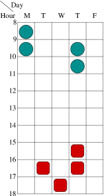
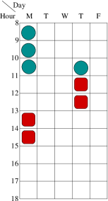
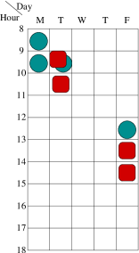
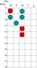
Figure 1: Timetable 1, 2, 3 and 4

Another real example could be the problem of compatibility of a couple of shifts in a work place. For example teachers that work in different class timetables, telephone operators, etc. Imagine a company where the work is divided in shifts of 4 hours per week. Many workers have to combine a couple of shifts in the same week and a predicate $compatible/2$ is necessary to check if two shifts are compatible or to obtain which couples of shifts are compatible. Two shifts are compatible when both are correct (working days from Monday to Friday, hours between 8 a.m. and 18 p.m. and there are no repetitions of the same hour in a shift) and in addition when the shifts are disjoint.

compatible(T1,T2):- correct_shift(T1), correct_shift(T2),
                    disjoint(T1,T2).

But there are so many compatible combinations of shifts that it would be useful to define the concept of compatibility in a fuzzy way instead of in the crisp way it is defined above. It would express that two shifts could be incompatible if one of them is not correct or if they are not disjoint but when they are compatible, they can be more or less compatible. They can have a level of compatibility. Two shifts will be more compatible if the working hours are concentrated (the employee has to go to work few days during the week). Also, two shifts will be more compatible if there are few free hours between the busy hours of the working days of the timetable.

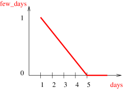
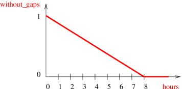
Figure 2: Fuzzy predicates few_days/2 and without_gaps/2

Therefore, we are handling crisp concepts ($correct\_shift/1$, $disjoint/2$) besides fuzzy concepts ($without\_gaps/2$, $few\_days/2$). Their definitions, represented in figure 2, are expressed in our language in this simple way (using the operator “$\mathit{:\#}$” for function definitions and the reserved word “$\mathit{fuzzy\_predicate}$”):

few_days :#
   fuzzy_predicate([(0,1),(1,0.8),(2,0.6),(3,0.4),(4,0.2),(5,0)]).

without_gaps :#
   fuzzy_predicate([(0,1),(1,0.8),(5,0.3),(7,0.1),(8,0)]).

A simple implementation in Fuzzy Prolog combining both types of predicates could be:

compatible(T1,T2,V):~ min
        f_correct_shift(T1,V1),
        f_correct_shift(T2,V2),
        f_disjoint(T1,T2,V3),
        f_append(T1,T2,T,V4),
        f_number_of_days(T,D,V5),
        few_days(D,V6),
        f_number_of_free_hours(T,H,V7),
        without_gaps(H,V8).

Here $append/3$ gives the total weekly timetable of 8 hours from joining two shifts, $number\_of\_days/3$ obtains the total number of working days of a weekly timetable and $number\_of\_free\_hours/2$ returns the number of free one-hour gaps that the weekly timetable has during the working days. The $\verb#f_#\mathit{predicates}$ are the corresponding fuzzified crisp predicates. The aggregation operator $min$ will aggregate the value of $V$ from $V6$ and $V8$ checking that $V1$, $V2$, $V3$, $V4$, $V5$ and $V7$ are equal to $1$, otherwise it fails. Observe the timetables in figure 1. We can obtain the compatibility between the couple of shifts, T1 and T2, represented in each timetable asking the subgoal $compatible(T1,T2,V)$. The result is $V=0.2$ for the timetable 1, $V=0.6$ for the timetable 2, and $V=0$ for the timetable 3 (because the shifts are incompatible).

Regarding compatibility of shifts in a weekly timetable, we are going to ask some questions about the shifts T1 and T2 of timetable 4 of figure 1. One hour of T2 is not fixed yet.

We can note: the days of the week as $mo$, $tu$, $we$, $th$ and $fr$; the slice of time of one hour as the time of its beginning from $8$ a.m. till $17$ p.m.; one hour of the week timetable as a pair of day and hour and one shift as a list of 4 hours of the week.

If we want to know how to complete the shift T2 given a level of compatibility higher than 70 %, we obtain the slice from 10 to 11 p.m. at Wednesday or Monday morning.

?- compatible([(mo,9), (tu,10), (we,8), (we,9)],
              [(mo,8), (we,11), (we,12), (D,H)], V),
   V .>. 0.7 .

V = 0.9,  D = we, H = 10 ? ;
V = 0.75, D = mo, H = 10 ? ;
no

6 Conclusions and Future work

Extending the expressivity of programming systems is very important for knowledge representation. We have chosen a practical and extended language for knowledge representation: Prolog.

Fuzzy Prolog presented in [9] is implemented over Prolog instead of implementing a new resolution system. This gives it a good potential for efficiency, more simplicity and flexibility. For example aggregation operators can be added with almost no effort. This extension to Prolog is realized by interpreting fuzzy reasoning as a set of constraints [36], and after that, translating fuzzy predicates into CLP(${\cal R}$) clauses. The rest of the computation is resolved by the compiler.

In this paper we propose to enrich Prolog with more expressivity by adding default reasoning and therefore the possibility of handling incomplete information that is one of the most worrying characteristics of data (i.e. all information that we need usually is not available but only one part of the information is available) and anyway searches, calculations, etc. should be done just with the information that we had.

We have developed a complete and sound semantics for handling incomplete fuzzy information and we have also provided a real implementation based in our former Fuzzy Prolog approach.

We have managed to combine crisp information (CWA) and fuzzy information (OWA or default) in the same program. This is a great advantage because it lets us model many problems using fuzzy programs. So we have extended the expressivity of the language and the possibility of applying it to solve real problems in which the information can be defined, fuzzy or incomplete.

Presently we are working in several related issues:

• Obtaining constructive answers to negative goals.

• Constructing the syntax to work with discrete fuzzy sets and its applications (recently published in [21]).

• Implementing a representation model using unions instead of using backtracking.

• Introducing domains of fuzzy sets using types. This seems to be an easy task considering that we are using a modern Prolog [10] where types are available.

• Implementing the expansion over other systems. We are studing now the advantages of an implementation in XSB system where tabling is used.

• Using our approach for the engine of robots in a RoboCup league in a joint project between our universities.

References

- [1] D. Cabeza and M. Hermenegildo. A New Module System for Prolog. In CL2000, number 1861 in LNAI, pages 131–148. Springer-Verlag, July 2000.
- [2] T.H. Cao. Annotated fuzzy logic programs. Fuzzy Sets and Systems, 113(2):277–298, 2000.
- [3] K. L. Clark. Negation as failure. In H. Gallaire and J. Minker, editors, Logic and Data Bases, pages 293–322, New York, NY, 1978. Plenum Press.
- [4] D. Dubois, J. Lang, and H. Prade. Towards possibilistic logic programming. In Proc. of ICLP-91, pages 581–595. MIT Press, 1991.
- [5] M. Fitting. Bilattices and the semantics of logic programming. Journal of Logic Programmig, 11:91–116, 1991.
- [6] N. Fuhr. Probabilistic datalog: Implementing logical information retrieval for advanced applications. Journal of the American Society for Information Science, 51(2):95–110, 2000.
- [7] M. Gelfond and V. Lifschitz. The stable model semantics for logic programming. In Fifth International Conference and Symposium on Logic Programming, pages 1070–1080, 1988.
- [8] M. Gelfond and V. Lifschitz. Logic programs with classical negation. In Seventh International Conference on Logic Programming, pages 579–597, Jerusalem, Israel, 1990. MIT Press. Extended abstract. (Complete version in ”New Generation Computing” 9:365-387,1991).
- [9] S. Guadarrama, S. Munoz-Hernandez, and C. Vaucheret. Fuzzy Prolog: A new approach using soft constraints propagation. Fuzzy Sets and Systems, FSS, 144(1):127–150, 2004. ISSN 0165-0114.
- [10] M. Hermenegildo, F. Bueno, D. Cabeza, M. Carro, M. García de la Banda, P. López-García, and G. Puebla. The CIAO Multi-Dialect Compiler and System: An Experimentation Workbench for Future (C)LP Systems. In Parallelism and Implementation of Logic and Constraint Logic Programming, pages 65–85. Nova Science, Commack, NY, USA, April 1999.
- [11] J. Jaffar and J. L. Lassez. Constraint Logic Programming. In ACM Symp. Principles of Programming Languages, pages 111–119. ACM, 1987.
- [12] J. Jaffar, S. Michaylov, P. J. Stuckey, and R. H. C. Yap. The clp(r) language and system. ACM Transactions on Programming Languages and Systems, 14(3):339–395, 1992.
- [13] M. Kifer and Ai Li. On the semantics of rule-based expert systems with uncertainty. In Proc. of ICDT-88, number 326 in LNCS, pages 102–117, 1988.
- [14] M. Kifer and V.S. Subrahmanian. Theory of generalized annotated logic programming and its applications. Journal of Logic Programming, 12:335–367, 1992.
- [15] E.P. Klement, R. Mesiar, and E. Pap. Triangular norms. Kluwer Academic Publishers.
- [16] L. Lakshmanan. An epistemic foundation for logic programming with uncertainty. LNCS, 880:89–100, 1994.
- [17] L. Lakshmanan and N. Shiri. Probabilistic deductive databases. Int. Logic Programming Symposium, pages 254–268, 1994.
- [18] L. Lakshmanan and N. Shiri. A parametric approach to deductive databases with uncertainty. IEEE Transactions on Knowledge and Data Engineering, 13(4):554–570, 2001.
- [19] Y. Loyer and U. Straccia. Uncertainty and partial non-uniform assumptions in parametric deductive databases. In Proc. of JELIA-02, volume 2424 of LNCS, pages 271–282, 2002.
- [20] T. Lukasiewicz. Fixpoint characterizations for many-valued disjunctive logic programs with probabilistic semantics. In Proc. of LPNMR-01, volume 2173, pages 336–350, 2001.
- [21] S. Munoz-Hernandez and J.M. Gómez Pérez. Solving collaborative fuzzy agents problems with clp(fd). In Manuel Hermenegildo and Daniel Cabeza, editors, International Symposium on Practical Aspects of Declarative Languages, PADL 2005, volume 3350 of LNCS, pages 187–202, Long Beach, CA (USA), 2005. Springer-Verlag.
- [22] R. Ng and V.S. Subrahmanian. Stable model semantics for probabilistic deductive databases. In Proc. of ISMIS-91, number 542 in LNCS, pages 163–171, 1991.
- [23] R. Ng and V.S. Subrahmanian. Probabilistic logic programming. Information and Computation, 101(2):150–201, 1993.
- [24] H. T. Nguyen and E. A. Walker. A first Course in Fuzzy Logic. Chapman & Hall/Crc, 2000.
- [25] A. Pradera, E. Trillas, and T. Calvo. A general class of triangular norm-based aggregation operators: quasi-linear t-s operators. International Journal of Approximate Reasoning, 30(1):57–72, 2002.
- [26] V.S. Subrahmanian. On the semantics of quantitative logic programs. In Proc. of 4th IEEE Symp. on Logic Programming, pages 173–182. Computer Society Press, 1987.
- [27] A. Tarski. A lattice-theoretical fixpoint theorem and its applications. Pacific Journal of Mathematics, 5:285–309, 1955.
- [28] E. Trillas, S. Cubillo, and J. L. Castro. Conjunction and disjunction on . Fuzzy Sets and Systems, 72:155–165, 1995.
- [29] E. Trillas, A. Pradera, and S. Cubillo. A mathematical model for fuzzy connectives and its application to operator´s behavioural study. In B. Bouchon-Meunier, R.R. Yager, and L.A. Zadeh, editors, Information, Uncertainty and Fusion, volume 516, pages 307–318. Kluwer Academic Publishers (Series: The Kluwer International Series in Engineering and Computer Sciences), 1999.
- [30] M.H. van Emden. Quantitative duduction and its fixpoint theory. Journal of Logic Programming, 4(1):37–53, 1986.
- [31] C. Vaucheret, S. Guadarrama, and S. Munoz-Hernandez. Fuzzy prolog: A simple implementation using clp(r). In Constraints and Uncertainty, Paphos (Cyprus), 2001. CP’2001 workshop. http://www.clip.dia.fi.upm.es/clip/papers/fuzzy-lpar02.ps.
- [32] C. Vaucheret, S. Guadarrama, and S. Munoz-Hernandez. Fuzzy prolog: A simple general implementation using clp(r). In M. Baaz and A. Voronkov, editors, Logic for Programming, Artificial Intelligence, and Reasoning, LPAR 2002, number 2514 in LNAI, pages 450–463, Tbilisi, Georgia, October 2002. Springer-Verlag.
- [33] G. Wagner. A logical reconstruction of fuzzy inference in databases and logic programs. In Proc. of IFSA-97, Prague, 1997.
- [34] G. Wagner. Negation in fuzzy and possibilistic logic programs. In Logic programming and Soft Computing. Research Studies Press, 1998.
- [35] Ehud Y. and Shapiro. Logic programs with uncertainties: A tool for implementing rule-based systems. In IJCAI, pages 529–532, 1983.
- [36] L. Zadeh. Fuzzy sets as a basis for a theory of possibility. Fuzzy Sets and Systems, 1(1):3–28, 1978.