Technical Report IDSIA-18-05  
Universal Learning of Repeated Matrix Games
 

Abstract

We study and compare the learning dynamics of two universal learning algorithms, one based on Bayesian learning and the other on prediction with expert advice. Both approaches have strong asymptotic performance guarantees. When confronted with the task of finding good long-term strategies in repeated $2\times 2$ matrix games, they behave quite differently.

1 Introduction

Today, Data Mining and Machine Learning is typically treated in a problem-specific way: People propose algorithms to solve a particular problem (such as learning to classify points in a vector space), they prove properties and performance guarantees of their algorithms (e.g. for Support Vector Machines), and they evaluate the algorithms on toy or real data, with the (potential) aim to use them afterwards in real-world applications. In contrast, it seems that universal learning, i.e. a single algorithm which is applied for all (or at least “many”) problems, is neither feasible in terms of computational costs nor competitive in (practical) performance. Nevertheless, understanding universal learning is important: On the one hand, its practical success would lead a way to Artificial Intelligence. On the other hand, principles and ideas from universal learning can be of immediate use, and of course Machine learning research aims at exploring and establishing more and more general concepts and algorithms.

Because of its practical restrictions, most of the understanding of universal learning so far is theoretical. Some approaches which have been suggested in the past are (adaptive) Levin search [Lev73, WS96], Optimal Ordered Problem Solver [Sch02, Sch04] and Reinforcement Learning with split trees [Rin94, McC95] among others. For a thorough discussion see e.g. [Hut04]. In this paper, we concentrate on two approaches with very strong theoretical guarantees in the limit: the AI$\xi$ agent based on Bayesian learning [Hut02] and FoE based on Prediction with expert advice [PH05].

Both models work in the setup of a sequential decision problem: An agent interacts with an environment in discrete time $t$. At each time step, the agent does some action and receives a feedback from the environment. The feedback consists of a loss (or reward) plus maybe more information. (It is usually just a matter of convenience if losses or rewards are considered, as one can be transformed into the other by reverting the sign. Accordingly, in this paper we switch between both, always preferring the more convenient one.) In addition to this instantaneous loss (or reward), we will also consider the cumulative loss which is the sum of the instantaneous losses from $t=1$ up to the current time step, and the average per round loss which is the cumulative loss divided by the total number of time steps so far.

Most learning theory known so far concentrates on passive problems, where our actions have an influence on the instantaneous loss, but not on the future behavior of the environment. All regression, classification, (standard) time-series prediction tasks, common Bayesian learning and prediction with expert advice, and many others fall in this category. In contrast, here we deal with active problems. The environment may be reactive, i.e. react to our actions, which is the standard situation considered in Reinforcement Learning. These cases are harder in theory, and it is often impossible to obtain relevant performance bounds in general.

Both approaches we consider and compare are based on finite or countably infinite base classes. In the Bayesian decision approach, the base class consists of hypotheses or models for the environment. A model is a complete description of the (possibly probabilistic) behavior of the environment. In order to prove guarantees, it is usually assumed that the true environment is contained in the model class. Experts algorithms in contrast work with a class of decision-makers or experts. Performance guarantees are proven without any assumptions in the worst case, but only relative to the best expert in the class. In both approaches, the model class is endowed with a prior. If the model class is finite and contains $n$ elements, it is common to choose the uniform prior $\frac{1}{n}$. For universal learning it turns out that universal base classes for both approaches can be constructed from the set of all programs on some fixed universal (prefix) Turing machine. Then each program naturally corresponds to an element in the base class, and a prior weight is defined by $w(\mbox{{program}})=2^{-\mbox{\scriptsize{length}({program})}}$ (provided that the input tape of the Turing machine is binary). The prior is a (sub-)probability distribution on the class, i.e. $\sum w\leq 1$.

Contents. The aim of this paper is to better understand the actual learning dynamics and properties of the two universal approaches, which are both “universally optimal” in a sense specified later. Clearly, the universal base class is computationally very expensive or infeasible to use. So we will restrict on simpler base classes which are “universal” in a much weaker sense: we will employ complete Markov base classes where each element sees only the previous time step. Although these classes are not truly universal, they are general enough (and not tailored towards our applications), such that we expect the outcome to be a good indication for the dynamics of true universal learning. The problems we study in this paper are $2\times 2$ matrix games. (Due to lack of space, we will not go into the deep literature on learning equilibria in matrix games, as our primary interest the universal learning dynamics.) Matrix games are simple enough such that a “universal” algorithm with our restricted base class can learn something, yet they provide interesting and nontrivial cases for reactive environments, where really active learning is necessary. Moreover, in this way we can set up a direct competition between the two universal learners. The paper is structured as follows: In the next two sections, we present both universal learning approaches together with their theoretical guarantees. Section 4 contains the simulations, followed by a discussion in Section 5.

2 Bayesian Sequential Decisions (AI$\xi$)

Passive problems. Every inductive inference problem can be brought into the following form: Given a string $x_{<t}=x_{1:t-1}:=x_{1}x_{2}...x_{t-1}$, guess its continuation $x_{t}$. Here and in the following we assume that the symbols $x_{t}$ are in a finite alphabet $\mathcal{X}$, for concreteness the reader may think of $\mathcal{X}=\{0,1\}$. If strings are sampled from a probability distribution $\mu:\mathcal{X}^{*}\to[0,1]$, then predicting according to $\mu(x_{t}|x_{<t})$, the probability conditioned on the history, is optimal. If $\mu$ is unknown, predictions may be based on an approximation of $\mu$. This is what happens in Bayesian sequential prediction: Let the model class ${{\cal M}}\!:=\!\{\mu_{1},\mu_{2},...\}$ be a finite or countable set of distributions on strings $\mu_{i}(x_{1:t}|y_{1:t})$ which are additionally conditionalized to the past actions $y_{<t}$. The actions are necessary for dealing with sequential decision problems as introduced above. We agree on the convention that the learner issues action $y_{t}$ before seeing $x_{t}$. Let $\{w_{1},w_{2},\ldots\}$ be a prior on ${\cal M}$ satisfying $\sum w_{i}\leq 1$. Then the Bayes mixture is the weighted average

$$\xi(x_{1:t}|y_{1:t})\!:=\!\!\sum\nolimits_{i}w_{i}\cdot\mu_{i}(x_{1:t}|y_{1:t}).$$

One can show that the $\xi$-predictions rapidly converge to the $\mu$-predictions almost surely, if we assume that ${\cal M}$ contains the true distribution: $\mu\!\in\!{\cal M}$. This is not a serious constraint if we include all computable probability distributions in ${\cal M}$. This universal model class corresponds to all programs on a fixed universal Turing machine (cf. the introduction and [Sol64, Hut04]).

In a passive prediction problem, the behavior of the environments $\mu_{i}$ do not depend on our actions $y_{1:t}$. Here we may interpret our action $y_{t}$ as the prediction of $x_{t}$. Assume that $\ell:(y_{t},x_{t})\mapsto[0,1]$ is a function defining our instantaneous loss. Then the average per round regret of $\xi$ tends to 0 at least at rate $t^{-{1}/{2}}$, precisely

$${\textstyle\frac{1}{t}}L^{\xi}_{1:t}\leq{\textstyle\frac{1}{t}}L^{\mu}_{1:t}+2\sqrt{\ln w_{\mu}^{-1}/t}.$$ (1)

Here, $L^{\xi}_{1:t}$ is the cumulative $\mu$-expected loss of the $\xi$-predictions. The $\xi$-prediction (and likewise the $\mu$-prediction) is chosen Bayes optimal for the given loss function: $y_{t}^{\xi}=\arg\min_{y_{t}}\sum_{x_{t}}\ell(y_{t},x_{t})\xi(x_{1:t}|y_{1:t})$. The difference $L^{\xi}_{1:t}-L^{\mu}_{1:t}$ is termed regret.

Active problems. If the environment is reactive, i.e. depends on our action, then it is easy to construct examples where the greedy Bayes optimal loss minimization is not optimal. Instead, the far-sighted AI$\xi$-agent chooses the action

$$y_{t}^{\xi,d}=\arg\min_{y_{t}}\!\sum_{x_{t}}...\min_{y_{t+d}}\!\sum_{x_{t+d}}\ell_{t:t+d}{\xi}(x_{1:t+d}|y_{1:t+d}).$$ (2)

where $\ell_{t:t+d}=\ell(y_{t:t+d},x_{t:t+d})=\sum_{s=t}^{t+d}\ell(y_{s},x_{s})$ and $d$ is the depth of the expectimin-tree the agent computes by means of (2). We refer to $t+d$ as the (current) horizon. If we knew the final time $T$ in advance and had enough computational resources, we could choose $d=T-t$ according to the fixed horizon $T$. Taking $d$ fixed and small (e.g. $d=8$) is computationally feasible, this is the moving horizon variant. However, this can cause consistency problems: A sequence of actions which is started some time step $t$ may not seem favorable any more in the next time step $t+1$ (since the horizon shifts), and thus is disrupted. We therefore also use an almost consistent horizon variant which takes $d=8$ in the first step, then $d=7$, and so on down to $d=2$, after which we start again with $d=8$. (Actually, we do not go down to $d=1$, since then the agent would be greedy, which can for instance disrupt consecutive runs of cooperation in the Prisoner’s dilemma, see below.) A theoretically very appealing alternative is to consider the future discounted loss and infinite depth, which is a solution of the Bellman equations. This can be found in [Hut04], together with more discussion and the proof of the following optimality theorem for AI$\xi$.

Theorem 1 (Performance of AI$\xi$)

If there exists a self-optimizing policy $\rho$ in the sense that its expected average loss ${\textstyle\frac{1}{T}}L_{1:T}^{\rho}$ converges for $T\to\infty$ to the optimal average ${\textstyle\frac{1}{T}}L_{1:T}^{\mu}$ for all environments $\mu\in{\cal M}$, then this also holds for the universal policy $\xi$, i.e.

$$\mbox{If }\exists\rho\forall\mu:{\textstyle\frac{1}{T}}L_{1:T}^{\rho}\;\stackrel{{\scriptstyle T\to\infty}}{{\longrightarrow}}\;{\textstyle\frac{1}{T}}L_{1:T}^{\mu}\quad\Rightarrow\quad{\textstyle\frac{1}{T}}L_{1:T}^{\xi}\;\stackrel{{\scriptstyle T\to\infty}}{{\longrightarrow}}\;{\textstyle\frac{1}{T}}L_{1:T}^{\mu}$$

function $\ell=A(s_{0},x_{<t},y_{<t},d)$ $\ell^{0}:=\ell(0,s_{0})$, $\ell^{1}:=\ell(1,s_{0})$ If $d>1$ Then For $a\in\{0,1\}$ For $s\in\{0,1\}$ $\ell^{(s,a)}:=A(s,[x_{<t}s_{0}],[y_{<t}a],d\!-\!1)$ $\ell^{a}:=\ell^{a}+\xi(s|s_{0},a,x_{<t},y_{<t})\cdot\ell^{(s,a)}$ Return $\min\{\ell^{0},\ell^{1}\}$

Figure 1: The AI$\xi$ recursion for known loss matrix $\ell$.

For $\tau=1,2,3,\ldots$ Sample $r_{\tau}\in\{0,1\}$ independ. s.t. $P[r_{\tau}=1]=\gamma_{\tau}$ If $r_{\tau}=0$ Then Invoke subroutine ${{\mbox{{F\kern-0.80002ptP\kern-0.80002ptL}}}}(\tau)$: Sample $q_{\tau}^{i}\stackrel{{\scriptstyle d.}}{{\sim}}\mbox{{Exp}}$ independently for $1\leq i\leq n$ Select $I_{\tau}^{{\mbox{\scriptsize{F\kern-1.04996ptP\kern-1.04996ptL}}}}=\arg\min\limits_{1\leq i\leq n}\{\eta_{\tau}\hat{\ell}^{i}_{<\tau}+\ln w^{i}-q_{\tau}^{i}\}$ $\langle$end of subroutine ${{\mbox{{F\kern-0.80002ptP\kern-0.80002ptL}}}}(\tau)\rangle$ Play $I_{\tau}^{{\mbox{\scriptsize{F\kern-0.91003pto\kern-0.91003ptE}}}}:=I_{\tau}^{{\mbox{\scriptsize{F\kern-1.04996ptP\kern-1.04996ptL}}}}$ for $B_{\tau}$ elementary time steps Set $\hat{\ell}_{\tau}^{i}=0$ for all $1\leq i\leq n$ Else Sample $I_{\tau}^{{\mbox{\scriptsize{F\kern-0.91003pto\kern-0.91003ptE}}}}\!\in\!\{1...n\}$ uniformly Play $I:=I_{\tau}^{{\mbox{\scriptsize{F\kern-0.91003pto\kern-0.91003ptE}}}}$ for $B_{\tau}$ elementary time steps Let $t_{0}(\tau):=\sum_{\tau^{\prime}=1}^{\tau-1}B_{\tau^{\prime}}$ and $\ell_{\tau}^{I}:=\sum_{t=t_{0}(\tau)+1}^{t_{0}(\tau)+B_{\tau}}\ell_{t}^{I}$ Let $\hat{\ell}_{\tau}^{I}=\ell_{\tau}^{I}n/\gamma_{t}$ and $\hat{\ell}_{\tau}^{i}=0$ for all $i\neq I$

Figure 2: The algorithm FoE. The parameters $\eta_{t}$, $\gamma_{t}$, and $B_{t}$ will be specified in Theorem 2.

Matrix games (as defined in Section 4) are straightforward in our setup. We just have to consider that the opponent, i.e. the environment, does not know our action $y_{t}$ when deciding its reaction $x_{t}$: $\mu_{i}(x_{t}|x_{<t},y_{1:t})=\mu_{i}(x_{t}|x_{<t},y_{<t})$. AI$\xi$ for $2\times 2$ matrix games can then be implemented recursively as shown in Figure 2, if we additionally assume that the environments are Markov players with two internal states, corresponding to the reaction $x_{t}$ they are playing. Since in step $t$, we don’t know $x_{t}$ yet, AI$\xi$ must evaluate both $\mbox{AIXIrec}(0,x_{<t},y_{<t},d)$ and $\mbox{AIXIrec}(1,x_{<t},y_{<t},d)$ and compute a weighted mixture for both possible actions $a=0,1$. As long as we do not yet know the loss matrix $\ell:(y_{t},x_{t})\mapsto[0,1]$ completely (which we assume to be deterministic), we additionally compute an expectation over all assignments of losses which are consistent with the history. To this aim, we pre-define a finite set $\mathcal{L}\subset\mathbb{N}$ which contains all possible losses. In the simulations below, we use $\mathcal{L}=\{0\ldots 4\}\cup\{-16\}$, where the actual losses are always in $\{0\ldots 4\}$ and the large negative value of $-16$ encourages the agent to explore as long as he doesn’t know the losses completely. This is for obtaining interesting results with moderate tree depth: otherwise, when the loss observed by AI$\xi$ is relatively low, AI$\xi$ would explore only with a large depth. This phenomenon is explained in detail in Section 4.

Markov Decision Processes (mdp) have probably been most intensively studied from all possible environments. In an mdp, the environmental behavior depends only on the last action and observation, precisely $\mu(x_{t}|x_{<t},y_{<t})=\mu(x_{t}|x_{t-1},y_{t-1})$ in case of a matrix game. For a $2\times 2$ game, a Markov player is modelled by a $2\times 2\times 2$ transition matrix. It turns out that the (uncountable) class of all transition matrices with a uniform prior admits a closed-form solution:

$$\xi(x_{t}|x_{<t},y_{<t})={N_{x_{t\!-\!1}\to x_{t}}^{y_{t\!-\!1}}\!+\!1\over N_{x_{t\!-\!1}\to 0}^{y_{t\!-\!1}}\!+\!N_{x_{t\!-\!1}\to 1}^{y_{t\!-\!1}}\!+\!2},$$

where $N_{x_{t\!-\!1}\to x_{t}}^{y_{t\!-\!1}}$ counts how often in the history the state $x_{t-1}$ transformed to state $x_{t}$ under action $y_{t-1}$. This is just Laplace’ law of succession [Hut04, Prob.2.11&5.14]. (Observe that $\xi$ is not Markov but depends on the full history.) Note that the $\xi$ posterior estimate changes along the expectimin tree (2). Disregarding this important fact as is done in Temporal Difference learning and variants would result in greedy policies who have to rescue exploration by ad-hoc methods (like $\varepsilon$-greedy). One can show that there exist self-optimizing policies $\tilde{p}$ for the class of ergodic mdps [Hut04]. Although the class of transition matrices contains non-ergodic environments, a variant of Theorem 1 applies, and hence the Bayes optimal policy $p^{\xi}$ is self-optimizing for ergodic Markov players (which we will exclusively meet). The intuitive reason is that the class is compact and the non-ergodic environments have measure zero.

3 Acting with Expert Advice (FoE)

Instead of predicting or acting optimally with respect to a model class, we may construct an agent from a class of base agents. We show how this can be accomplished for fully active problems. The resulting algorithm will radically differ from the AI$\xi$ agent.

Prediction with expert advice has been very popular in the last two decades. The base predictors are called experts. Our goal is to design a master algorithm which in each time step $t$ selects one expert $i$ and follows its advice (i.e. predicts as the expert does). Thereby, we want to keep the master’s regret $\ell_{1:T}^{\mbox{\scriptsize{master}}}-\ell_{1:T}^{*}$ small, where $\ell_{1:T}^{*}$ is the cumulative loss of the best expert in hindsight at time $T$. Usually, $T\geq 1$ not known in advance. The state-of-the-art experts algorithms achieve this: Loss bounds similar to (1) can be proven, with $\ell_{1:T}^{\mu}$ replaced by $\ell_{1:T}^{*}$ and $w^{\mu}$ replaced by the prior weight of the best expert in hindsight, $w^{*}$. These bounds hold in the worst case, i.e. without any assumption on the data generating process. In particular, the environment which provides the feedback may be an adaptive adversary. Since these bounds imply bounds in expectation in the Bayesian setting (with slightly larger constants than (1)), expert advice is in a sense the stronger prediction strategy.

In order to protect against adaptive adversaries, we need to randomize. In this work, we build on the Follow the Perturbed Leader FPL algorithm introduced by [Han57]. (For space constraints, we won’t discuss the more popular alternative of weighted sampling at all.) We don’t even need to be told the true outcome after the master’s decision. All we need for the analysis is learning the losses of all experts, which are bounded wlog. in $[0,1]$ (this is an important restriction which applies to all standard experts algorithms). In this way, the master’s actual decision is based on the past cumulative loss of the experts. A key concept is that we must prevent the master from learning too fast (or to slowly). This is achieved by introducing a learning rate $\eta_{t}$, which decreases to zero at an appropriate rate with growing $t$. Most of the literature assumes experts classes of finite size $n$ with uniform prior $\frac{1}{n}$, in particular when the learning rate $\eta_{t}$ is non-stationary. For FPL, the case of arbitrary non-uniform prior and countable expert classes has been treated in [HP04].

Active problems. In the passive full observation game discussed so far (i.e. we learn all losses), the notion of regret is not problematic even against an adaptive adversary. However, the situation changes if the reaction of the environment depends on our past actions. Consider the simple case of two experts, one always suggesting action 0 and the other one action 1. The environment is reactive and “unfair”: Each expert incurs no loss as long as we stay with its initial action (e.g. the action sequences 00000 and 111 have no loss). But as soon as we perform a different action (e.g. 001), in all subsequent rounds both experts incur loss 1. Each sensible strategy will soon explore both actions, and compared to the pure experts, we incur large loss. Consequently, we need to consider a different notion of regret: Our performance is compared to what an expert could achieve when he is actually put in our situation. In this example, after the action sequence 001, we perform badly, but so do all experts.

Another problem with reactive environments is that we do not necessarily get valid feedback for all experts in each round. In the previous example, if we chose 0 as the first action and learned that expert 0 had no loss at time $t=2$, it is not legitimate to make any assumption on the loss of expert 1 at $t=2$. Even if the environment tells us that the pure expert 1 had no loss, we are interested in the loss of expert 1 put in our situation, i.e. after the first action 0. But this loss we do not know. Precisely, we know only the loss of an expert with the correct action history after the last time step in the past, where we (maybe coincidentally) acted as he suggested. Instead of trying to track the action history (which is possibly expensive), we therefore use only the feedback from the currently selected expert $i$ and discard all other information. This is commonly referred to as bandit setup. Fortunately, this issue can be successfully addressed by forcing exploration, i.e. sampling according to the prior, with a certain probability $\gamma_{t}$ [MB04]. This exploration rate $\gamma_{t}$ is decreased to zero appropriately with growing $t$. Thus, in each time step we decide to either follow the perturbed leader or explore. Accordingly, we call our algorithm FoE (Follow or Explore). Bounds for the bandit setup are typically similar to (1), but with $-\ln w^{*}$ replaced by (something larger than) $1/w^{*}$. Hence they are exponentially larger in $w^{*}$, and one can show that this is sharp in general.

Increasing horizon. If the environment is reactive, it is not sufficient to consider only the short-term performance of the selected expert $i$. This was first recognized by [dFM04], who considered the repeated game of “Prisoner’s Dilemma” and the “tit for tat” opponent as a motivating example (see Section 4 for details). In this case, a good long term strategy is cooperating (because of the particular opponent). However defecting is dominant, i.e. the instantaneous loss of defecting is always smaller than that of cooperating. So in order to notice that an expert (for instance the always cooperating one) performs well, we have to evaluate it at least over two time steps. In general, if we evaluate a chosen expert over an increasing number of time steps, we hope that we perform well in arbitrary reactive environments. This means that the master works at a different time scale $\tau$: in its $\tau$th time step, it gives the control to the selected expert for $B_{\tau}\geq 1$ time steps (in the original time scale $t$). As a consequence, the instantaneous losses which the master observes are no longer uniformly bounded in $[0,1]$, but in $[0,B_{\tau}]$. Fortunately, it turns out that the analysis remains valid if $B_{\tau}$ grows unboundedly but slowly enough. Only the convergence rate of the average master’s loss to the optimum is affected: we will obtain a final rate of $t^{-{1}/{10}}$. The resulting algorithm FoE (for a finite expert class) is specified in Figure 2 together with its subroutine FPL. We may have instantaneous and cumulative losses in both time scales, this is always clear from the notation (e.g. $\ell^{i}_{t}$ vs. $\hat{\ell}_{<\tau}^{i}$). Not surprisingly, most of FoE works in the master time scale.

Note that FoE makes use of its observation only if he decided to explore, i.e. if $r_{\tau}=1$. This seems an unnecessary waste of information. This is motivated from the analysis, since FoE needs an unbiased loss estimate $\hat{\ell}$ (with respect to FoE’s randomization). We just chose the simplest way to guarantee this. For the simulations, we concentrate on the following faster learning variant: approximate the probability $p_{\tau}^{i}$ of the selected expert $i$ (jointly for exploration and exploitation) by a Monte-Carlo simulation. Then always learn a (close to) unbiased estimate $\hat{\ell}_{\tau}^{i}=\frac{\ell_{\tau}^{i}}{p_{\tau}^{i}}$. The analysis of FoE works in the same way for this modification, however not resulting in better bounds. On the other hand, we will see that modified FoE learns faster.

In case of a non-uniform prior and possibly infinitely many experts, the exploration must be according to the prior weights. This causes another problem: FoE’s loss estimates $\hat{\ell}$ need to be bounded, which forbids exploring experts with very small prior weights. Hence we define for each expert $i$, an entering time $\mathcal{T}^{i}\geq 1$ (at the master time scale). Then FoE (including its subroutine FPL) is modified such that it uses only active experts from $\{i:\tau\geq\mathcal{T}^{i}\}$. This guarantees additionally that we have only a finite active set in each step, and the algorithm remains computationally feasible.

Theorem 2 (Performance of FoE)

Assume FoE acts in an online decision problem with bounded instantaneous losses $\ell_{t}^{i}\in[0,1]$. Let the exploration rate be $\gamma_{\tau}=\tau^{-{1}/{4}}$ and the learning rate be $\eta_{\tau}=\tau^{-{3}/{4}}$. In case of uniform prior, choose $B_{\tau}=\lfloor\tau^{{1}/{8}}\rfloor$. In case of arbitrary prior let $B_{\tau}=\lfloor t^{{1}/{16}}\rfloor$ and $\mathcal{T}^{i}=\lceil(w^{i})^{-16}\rceil$. Then in case of uniform prior, for all experts $i$ and all $T\geq 1$ we have

$${\textstyle\frac{1}{T}}{\mathbf{E}}\ell^{{\mbox{\scriptsize{F\kern-0.91003pto\kern-0.91003ptE}}}}_{1:T} \leq {\textstyle\frac{1}{T}}\ell_{1:T}^{i}+O(n^{2}T^{-{1}/{10}}),\mbox{ and }$$

$${\textstyle\frac{1}{T}}\ell^{{\mbox{\scriptsize{F\kern-0.91003pto\kern-0.91003ptE}}}}_{1:T} \leq {\textstyle\frac{1}{T}}\ell_{1:T}^{i}+O(n^{2}T^{-{1}/{10}})\mbox{ w.p. }1-T^{-2}.$$

Consequently, $\limsup_{T\to\infty}{\textstyle\frac{1}{T}}(\ell^{{\mbox{\scriptsize{F\kern-0.91003pto\kern-0.91003ptE}}}}_{1:T}-\ell^{i}_{1:T})\leq 0$ a.s. For non-uniform prior, corresponding assertions hold with $O$-terms replaced by $O\big{(}T^{-{1}/{10}}+(w^{i})^{-22}T^{-1}\big{)}$.

The proof of this main theorem on the performance of FoE can be found in [PH05]. Similar bounds hold for larger $B_{\tau}<\tau^{\frac{1}{4}}$. These bounds are improvable [Pol05], and it is possible to prove any regret bound $O\Big{(}(\frac{1}{w^{i}})^{c}+(\log\frac{1}{w^{i}})T^{\frac{2}{3}+\varepsilon}\Big{)}$, at the cost of increasing $c$ where $\varepsilon\to 0$. In the simulations, we used $B_{\tau}=\tau^{0.24}$ for faster learning. For playing $2\times 2$ matrix games, we will use the class of all 16 deterministic four-state Markov experts. That is, each expert consists of a lookup table with all the actions for each of the 4 possible combination of moves in the last round. In the first round, the expert plays uniformly random. (Compare the standard results on learning matrix games with expert advice by [FS99].)

4 Simulations

As already indicated, it is our goal to explore and compare the performance of the two universal learning approaches presented so far, in particular for problems which are not solved by passive or greedy learners. To this aim, repeated $2\times 2$ matrix games are well suited:

• they are simple, such that (close to) universal learning is computationally feasible even with brute-force implementation;

• they provide situations where optimal long-term behavior significantly differs from greedy behavior (e.g. Prisoner’s Dilemma);

• moreover, we can observe how universal learners can exploit potentially weak adversaries;

• and finally, we can test the two universal learners against each other.

We begin by describing the experimental setup and the universal learners. After that, we will discuss five $2\times 2$ matrix games, presenting experimental results and highlighting their interesting aspects.

Setup. A $2\times 2$ matrix game consists of two matrices $R_{1},R_{2}\in\mathbb{R}^{2\times 2}$, the first one containing rewards for the row player, the second one rewards for the column player. (It does not cause any problem that for convenience, we have developed the theory in terms of losses rather than rewards: one may be transformed into the other by simply inverting the sign. So for the discussion of the results, we will keep the rewards, as this is more standard in game theory.) A single game proceeds in the following way: the first player chooses a row action $i\in\{0,1\}$ and simultaneously the second a column action $j\in\{0,1\}$, both players without knowing the opponent’s move. Then reward $R_{k}(i,j)$ is payed to player $k$ ($k=1,2$), and $i$ and $j$ are revealed to both players. A repeated game consists of $T$ single games. We chose $T=20000$, if at least one opponent is FoE (which has slow learning dynamics, as we will see), and $T=100$ for the fast learning AI$\xi$ (unless it is plotted in the same graph as FoE). If at least one randomized player participates, the run is repeated 10 times, and usually the average is shown. We will consider only symmetric games, where one player, when put in the position of the other player (i.e. when exchanging $R_{1}$ and $R_{2}$), has a symmetric strategy (maybe after exchanging the actions). We will meet precisely three types of symmetry: in the “Matching Pennies”, $R_{1}=R_{2}$ after inverting the action of the row player, and in the “Battle of Sexes” game, $R_{1}=R_{2}$ after inverting both players’ actions, and in all other games we $R_{1}=R_{2}^{T}$ (transpose). In these latter games, we will call the action 0 “defect” and 1 “cooperate”. All games we consider have rewards in $\{0\ldots 4\}$. The AI$\xi$ and FoE agents are used as specified in the previous sections, with the classes of all two-state Markov environments and all deterministic four-state Markov experts, respectively. For AI$\xi$, we will concentrate the presentation on the almost consistent horizon variant, since it performs always better than the moving horizon variant. For FoE, we will concentrate on the faster learning variant.

	0	1
0	1,1	4,0
1	0,4	2,3
Prisoner’s Dilemma

	0	1
0	2,2	3,0
1	0,3	4,4
Stag Hunt

	0	1
0	0,0	4,1
1	1,4	2,2
Chicken

	0	1
0	2,4	0,0
1	0,0	4,2
Battle of Sexes

	0	1
0	4,0	0,4
1	0,4	4,0
Matching Pennies

Figure 3: Reward Matrices

Prisoner’s Dilemma. This dilemma is classical. The reward matrices are $R_{1}={14\choose 03}$ and $R_{2}=R_{1}^{T}$, with the following interpretation: The two players are accused of a crime they have committed together. They are being interrogated separately. Each player can either cooperate with the other player (don’t tell the cops anything), or he defects (tells the cops everything but blame the colleague). The punishments are according to the players’ joint decision: if none of them gives evidence, both get a minor sentence. If one gives evidence and the other one keeps quiet, the traitor gets free, while the other gets a huge sentence. If both give evidence, then they both get a significant sentence. (There is also an easier variant “Deadlock” which we not discuss.)

It is clear that giving evidence, i.e. defecting, is an instantaneously dominant action: regardless of what the opponent does, the immediate reward is always larger for defecting. However, if both players would agree to cooperate, this is the “social optimum” and guarantees the better long-term reward in the repeated game. A well-known instance for this case is playing against the “tit for tat” strategy strategy which cooperates in the first move and subsequently performs the action we did in the previous move. Similar but harder to learn are “two tit for tat” and “three tit for tat”, which defect in the first move and cooperate only if we cooperated two respectively three times in a row. Note that although “two tit for tat” and “three tit for tat” are not in AI$\xi$’s model class, probabilistic versions of the strategies are: if the probability of “adversary defected, I cooperate, then the adversary will cooperate in the next round” is chosen correctly (namely $\frac{1}{2}$ for 2-tit for tat and $\approx 0.57$ for 3-tit for tat), then the expected number of rounds I have to cooperate until the adversary will do so is 2 respectively 3.

Figure 5 shows that in most cases, AI$\xi$ learns very quickly the best actions. (This is the consistent horizon variant, the moving horizon variant will be discussed with the next game, Stag Hunt.) If the opponent is memoryless as for example the uniform random player, AI$\xi$ constantly defects after short time. Against tit for tat and two tit for tat, AI$\xi$ cooperates after short time. The figure shows the average per round rate of cooperation, which after a few exploratory moves converges to the optimal action as $\frac{1}{t}$. However, AI$\xi$ does not learn to cooperate against three tit for tat. The reason is the general problem that in order to increase exploration, AI$\xi$ needs exponential depth of the expectimin tree. Assume that a certain action sequence of length $n$ is favorable against the true environment, which has however not too high a current weight. In this instance, cooperating three times in a row is favorable against (the probabilistic version of) 3-tit for tat. In order to recognize that this is worth exploring, AI$\xi$ has to build a branch of depth $n=3$ in the expectimin tree, which has (because of the relatively low prior weight) very small probability $\sim\exp(-n)$ however. Then it needs an exponentially large subtree below this branch to accumulate enough (virtual) reward in order to encourage exploration.

One more problem arises when AI$\xi$ plays against another AI$\xi$. Here, the perfectly symmetric setting results in both playing the same actions in each move, hence they are not correctly learning. We might try to remedy this by varying the tree depth of the second AI$\xi$ (denoted AI$\xi$2 in the figure), however it turns out that in this case, both AI$\xi$’s do not learn at all to cooperate (see [Hut04, Sec.8.5.2] for a possible reason).

We now turn to the performance of FoE (the faster learning variant) as evaluated in Figure 5. As expected, FoE learns much slower than AI$\xi$ (note the different time scale). On the other hand, its exploration is strong enough to learn 3-tit for tat (and even harder instances). When playing against another instance of FoE, we notice however that they usually do not succeed to overcome the dominance of mutual defection. Also when FoE competes with AI$\xi$, they tend to learn mutual defection rather than cooperation. (Sometimes, they learn cooperation in one or two of the possible states of the MDP.)

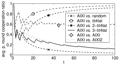
Figure 4: AI$\xi$ in Prisoner’s Dilemma

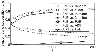
Figure 5: FoE (and AI$\xi$) in Prisoner’s Dilemma

Stag Hunt. This game is also known as “Assurance”. The reward matrices are $R_{1}={23\choose 04}$ and $R_{2}=R_{1}^{T}$. Two players are hunting together. If they cooperate, they will catch the stag. However, one player might not trust the other, in which case he chases rabbits on his own instead. In this case, the other one won’t get anything if he tries to cooperate. If both defect, then they are in conflict, and each player gets less rabbits. Although the optimum for both players is to cooperate, they need to trust each other sufficiently. If one player plays uniformly random, it is better for the other to go for the rabbits. Also, defecting has the lower variance.

Maybe it is surprising to observe that AI$\xi$ (with a depth of 8) does not learn to cooperate against 2-tit for tat (Figure 7). The reason is that defecting has a relatively good payoff, and therefore exploration is not encouraged as discussed in the previous subsection. If the depth of the tree is increased to 9, AI$\xi$ learns cooperation against 2-tit for tat (but not against 3-tit for tat). We also see that the moving horizon variant of AI$\xi$ has even more problems with exploration: It does not learn cooperating against 2-tit for tat, even with depth 9. The explanation is that even if AI$\xi$ decides to explore in one time step, in the next step this exploration might not be correctly continued, as the tree is now explored to a different level. This observation can also be made for the Prisoner‘s Dilemma. In fact, the consistent horizon variant performs always better than moving horizon.

As before, FoE learns much slower but explores more robustly (Figure 7), neither 2- nor 3-tit for tat are a problem. Unlike in the Prisoner’s Dilemma, if AI$\xi$ and FoE are competing, they learn mutual cooperation in almost half of the cases, an average over such lucky instances is given in the figure. The same is valid for FoE against FoE, while AI$\xi$ against AI$\xi$ has the same symmetry problem as already observed in the Prisoner’s Dilemma. The original slower learning variant of FoE reaches the same average level of performance only after $10^{5}$ time steps instead of $2\cdot 10^{4}$ steps, and moreover with a variance twice as high.

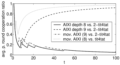
Figure 6: Stag Hunt: AI$\xi$ and its moving horizon variant

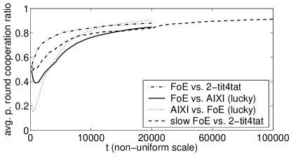
Figure 7: Stag Hunt: FoE and its slower learning variant

Chicken. The reward matrices $R_{1}={04\choose 12}$ and $R_{2}=R_{1}^{T}$ of the “Chicken” game (also known as “Hawk and Dove”) can be interpreted as follows: Two coauthors write a paper, but each tries to spend as little effort as possible. If one succeeds to let the other do the whole work, he has a high reward. On the other hand, if no one does anything, there will be no paper and thus no reward. Finally, if both decide to cooperate, both get some reward. Here, in the repeated game, it is socially optimal to take turns cooperating and defecting. Still the best situation for one player is if he emerges as the “dominant defector”, defecting in most or all of the games, while the other one cooperates.

If the opponent steadily alternates between cooperating and defecting, then AI$\xi$ quickly learns to adapt. This can be observed in Figure 9, where the performance is given in terms of average per round reward instead of cooperation rate. However, AI$\xi$ is not obstinate enough to perform well against a “stubborn” adversary that would cooperate only after his opponent has defected for three successive time steps. Here, AI$\xi$ learns to cooperate, leaving his opponent the favorable role as the dominant defector. (However, AI$\xi$ learns to dominate the less stubborn adversary which cooperates after two defecting actions.) When two AI$\xi$s play against each other, they again have the symmetry problem. Interestingly, if we break symmetry by giving the second AI$\xi$ a depth of 9, he will turn out the dominant defector (not shown in the graph).

FoE behaves differently in this game (Figure 9). While he learns to deal with the steadily alternating adversary and emerges as the dominant defector against the stubborn one, he would give precedence to AI$\xi$ in most cases. This is not hard to explain, since FoE in the beginning plays essentially random. Thus AI$\xi$ learns quickly to defect, and for FoE remains nothing but learning to cooperate. However, this does not always happen: In the minority of the cases, FoE defects enough such that AI$\xi$ decides to cooperate, and FoE will be the dominant defector. (Hence the average shown in the graph is less clear in favor of AI$\xi$.)

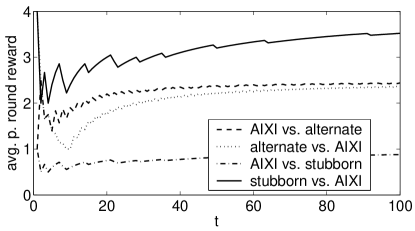
Figure 8: AI$\xi$ in the Chicken game

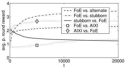
Figure 9: FoE (and AI$\xi$) in the Chicken game

Battle of Sexes. In this game, a married couple wants to spend the evening together, but they didn’t settle if they would go to the theater (her preference) or the pub (his preference). However, if they fail to meet, both have a boring evening (and no reward at all). The reward matrices are $R_{1}={20\choose 04}$ and $R_{2}={40\choose 02}$. Coordination is clearly important in the repeated game. Like in “Chicken”, taking turns is a social optimum, while it is best for one player if his choice becomes dominant.

In Figure 11, our universal learners show similar performance like in the Chicken game. Both learn to deal with an alternating partner. FoE also learns to dominate over a stubborn adversary which plays his less favorite action only after the opponent insists three times on that. AI$\xi$ is dominated by this stubborn player. However, AI$\xi$ always dominates FoE. Finally, in contrast to the Chicken game, AI$\xi$ against AI$\xi$ does not have the symmetry problem, but they both learn to alternate.

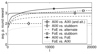
Figure 10: AI$\xi$ and FoE in Battle of Sexes

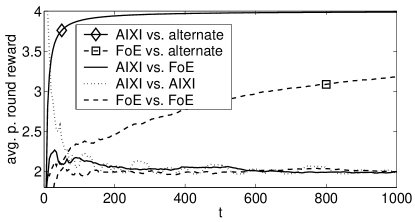
Figure 11: AI$\xi$ and FoE in Matching Pennies

Matching Pennies. Each player conceals in his palm a coin with either heads or tails up. They are revealed simultaneously. If they match (both heads or both tails), the first player wins, otherwise the second. This is the only zero-sum game of the games we consider, where $R_{1}={40\choose 04}$ and $R_{2}={04\choose 40}$. Thus, there is a minimax strategy for both players, which is actually uniform random play. On the other hand, deterministic repeated play is potentially exploitable by the adversary.

Figure 11 shows the results for this last game we present. Both AI$\xi$ and FoE learn to exploit a predictable adversary, namely the player alternating between 0 and 1. The other games are balanced in the long run, only in the beginning AI$\xi$ succeeds to exploit FoE a little. If two AI$\xi$s compete, it is important to break symmetry, then both learn to alternate (this situation is shown in the graph). If symmetry is not broken, the row player (who tries to match) always wins.

5 Discussion

Altogether, universal learners perform well in repeated matrix games. They usually learn to prefer the optimal long-term action to greedy behavior (Prisoner’s Dilemma and Stag Hunt). If possible they are able to exploit a predictable adversary (Matching Pennies). And they learn good strategies when it is necessary to foresee the opponent’s action (Chicken and Battle of Sexes). Of the two approaches we presented and compared, AI$\xi$ learns much faster than FoE, but FoE explores more thoroughly. Of course, there is a trade-off between exploration and fast learning. Interestingly, it may depend on the adversary (and thus on the environment) if fast learning or exploration is the better long-term strategy: In Chicken and Battle of Sexes, AI$\xi$ profits against FoE by learning fast and dictating its preferred action, but looses against the stubborn opponent because of not exploring enough.

Acknowledgement. This work was supported by the Swiss NSF grant 2100-67712.

References

- [dFM04] D. Pucci de Farias and N. Megiddo. How to combine expert (and novice) advice when actions impact the environment? In Sebastian Thrun, Lawrence Saul, and Bernhard Schölkopf, editors, Advances in Neural Information Processing Systems 16. MIT Press, Cambridge, MA, 2004.
- [FS99] Y. Freund and R. Schapire. Adaptive game playing using multiplicative weights. Games and Economic Behavior, 29:79–193, 1999.
- [Gen03] C. Gentile. The robustness of the p-norm algorithm. Machine Learning, 53(3):265–299, 2003.
- [Han57] J. Hannan. Approximation to Bayes risk in repeated plays. In M. Dresher, A. W. Tucker, and P. Wolfe, editors, Contributions to the Theory of Games 3, pages 97–139. Princeton University Press, 1957.
- [HP04] M. Hutter and J. Poland. Prediction with expert advice by following the perturbed leader for general weights. In International Conference on Algorithmic Learning Theory (ALT), pages 279–293, 2004.
- [HP05] M. Hutter and J. Poland. Adaptive online prediction by following the perturbed leader. Journal of Machine Learning Research, 6:639–660, 2005.
- [Hut02] M. Hutter. Self-optimizing and Pareto-optimal policies in general environments based on Bayes-mixtures. In Proc. 15th Annual Conference on Computational Learning Theory (COLT 2002), Lecture Notes in Artificial Intelligence, pages 364–379, Sydney, Australia, July 2002. Springer.
- [Hut04] M. Hutter. Universal Artificial Intelligence: Sequential Decisions based on Algorithmic Probability. Springer, Berlin, 2004.
- [Lev73] L. A. Levin. Universal sequential search problems. Problems of Information Transmission, 9:265–266, 1973.
- [MB04] H. B. McMahan and A. Blum. Online geometric optimization in the bandit setting against an adaptive adversary. In 17th Annual Conference on Learning Theory (COLT), pages 109–123. Springer, 2004.
- [McC95] A. K. McCallum. Instance-based utile distinctions for reinforcement learning with hidden state. In Proc. 12th International Conference on Machine Learning, pages 387–395, 1995.
- [PH05] J. Poland and M. Hutter. Defensive universal learning with experts. 2005. International Conference on Algorithmic Learning Theory (ALT), to appear.
- [Pol05] J. Poland. FPL analysis for adaptive bandits. 2005. 3rd Symposium on Stochastic Algorithms, Foundations and Applications (SAGA), to appear.
- [Rin94] M. Ring. Continual Learning in Reinforcement Environments. PhD thesis, University of Texas at Austin, Austin, Texas., 1994.
- [Sch02] J. Schmidhuber. Bias-optimal incremental problem solving. In Advances in Neural Information Processing Systems 15. MIT Press, Cambridge, MA, 2002. To appear.
- [Sch04] J. Schmidhuber. Optimal ordered problem solver. Machine Learning, 54(3):211–254, 2004.
- [Sol64] R. J. Solomonoff. A formal theory of inductive inference: Part 1 and 2. Inform. Control, 7:1–22, 224–254, 1964.
- [WS96] M. Wiering and J. Schmidhuber. Solving POMDPs with Levin search and EIRA. In Machine Learning: Procceedings of 13th International Conference, pages 534–542, Bari, Italy, 1996.