DNA Codes that Avoid Secondary Structures

Abstract

In this paper, we consider the problem of designing codewords for DNA storage systems and DNA computers that are unlikely to fold back onto themselves to form undesirable secondary structures. Secondary structure formation causes a DNA codeword to become less active chemically, thus rendering it useless for the purpose of DNA computing. It also defeats the read-back mechanism in a DNA storage system, so that information stored in such a folded DNA codeword cannot be retrieved. Based on some simple properties of a dynamic-programming algorithm, known as Nussinov’s method, which is an effective predictor of secondary structure given the sequence of bases in a DNA codeword, we identify some design criteria that reduce the possibility of secondary structure formation in a codeword. These design criteria can be formulated in terms of the requirement that the Watson-Crick distance between a DNA codeword and a number of its shifts be larger than a given threshold. This paper addresses both the issue of enumerating DNA sequences with such properties and the problem of practical DNA code construction.

I Introduction

The last century was marked by the birth of two major scientific and engineering disciplines: silicon-based computing and the theory and technology of genetic data analysis. The research field very likely to dominate the area of scientific computing in the foreseeable future is the merger of these two disciplines, leading to unprecedented possibilities for applications in varied areas of engineering and science. The first steps toward this goal were made in 1994, when Leonard Adleman [1] solved a quite unremarkable computational problem, an instance of the directed travelling salesmen problem on a graph with seven nodes, with an exceptional method. The technique used for solving the problem was a new technological paradigm, termed DNA computing. DNA computing introduced the possibility of using genetic data to tackle computationally hard classes of problems that are otherwise impossible to solve using traditional computing methods. The way in which DNA computers make it possible to achieve this goal is through massive parallelism of operation on nano-scale, low-power, molecular hardware and software systems.

One of the major obstacles to efficient DNA computing, and more generally DNA storage [7] and signal processing [11], is the very low reliability of single-stranded DNA sequence operations. DNA computing experiments require the creation of a controlled environment that allows for a set of single-stranded DNA codewords to bind (hybridize) with their complements in an appropriate fashion. If the codewords are not carefully chosen, unwanted, or non-selective, hybridization may occur. Even more detrimental is the fact that a single-stranded DNA sequence may fold back onto itself, forming a secondary structure which completely inhibits the sequence from participating in the computational process. Secondary structure formation is also a major bottleneck in DNA storage systems. For example, it was reported in [7] that $30\%$ of read-out attempts in a DNA storage system failed due to the formation of special secondary structures called hairpins in the single-stranded DNA molecules used to store information.

So far, the focus of coding for DNA computing was exclusively directed towards constructing large sets of DNA codewords with fixed base frequencies (constant GC-content) and prescribed Hamming/reverse-complement Hamming distance. Such sets of codewords are expected to result in very rare hybridization error events. As an example, it was shown in [3] that there exist $94595072$ codewords of length $20$ with minimum Hamming distance $d=5$ and with exactly $10$ G/C  bases. At the same time, the Wisconsin DNA Group, led by D. Shoemaker, reported that through extensive computer search and experimental testing, only $9105$ sequences of length $20$ at Hamming distance at least $5$ were found to be free of secondary structure at temperatures of $61\pm 5^{o}C$. Since at lower ambient temperatures the probability of secondary structure formation is even higher, it is clear that the effective number of codewords useful for DNA computing is extremely small.

In this paper, we investigate properties of DNA sequences that may lead to undesirable folding. Our approach is based on analysis of a well-known algorithm for approximately determining DNA secondary structure, called Nussinov’s method. This analysis allows us to extract some design criteria that yield DNA sequences that are unlikely to fold undesirably. These criteria reduce to the requirement that the first few shifts of a DNA codeword have the property that they do not contain Watson-Crick complementary matchings with the original sequence. We consider the enumeration of sequences having the shift property and provide some simple construction strategies which meet the required restrictions. To the best of our knowledge, this is the first attempt in the literature aimed at providing a rigorous setting that links DNA folding properties to constraints on the primary structure of the sequences.

II DNA Secondary Structure: Properties and Code Design Issues

DNA of higher species consists of two complementary chains twisted around each other to form a double helix. Each chain is a linear sequence of nucleotides, or bases— two purines, adenine (A) and guanine (G), and two pyrimidines, thymine (T) and cytosine (C). The purine bases and pyrimindine bases are Watson-Crick (WC) complements of each other, in the sense that

$$\overline{\textbf{A}}=\textbf{T},\ \ \ \overline{\textbf{G}}=\textbf{C},\ \ \ \overline{\textbf{C}}=\textbf{G},\ \ \ \overline{\textbf{T}}=\textbf{A}.$$ (1)

More specifically, in a double helix, the base A pairs with T by means of two hydrogen bonds, while C pairs with G by means of three hydrogen bonds (i.e. the strength of the former bond is weaker than the strength of the latter). For DNA computing purposes, one is only concerned with single-stranded (henceforth, oligonucleotide) DNA sequences.

Oligonucleotide DNA sequences are formed by heating DNA double helices to denaturation temperatures, at which they break down into single strands. If the temperature is subsequently reduced, oligonucleotide strands with large regions of sequence complementarity can bind back together in a process called hybridization. Hybridization is assumed to occur only between complementary base pairs, and lies at the core of DNA computing.

As a first approximation, oligonucleotide DNA sequences can be simply viewed as words over a four-letter alphabet $Q=\{\textbf{A},\textbf{C},\textbf{G},\textbf{T}\}$, with a prescribed set of complex properties. The generic notation for such sequences will be $\mathbf{q}=q_{1}q_{2}\ldots q_{n}$, with $n$ indicating the length of the sequences. The WC complement $\overline{\textbf{q}}$ of a DNA sequence is defined as $\overline{q_{1}}\,\overline{q_{2}}\ldots\overline{q_{n}}$, $\overline{q_{i}}$ being the WC complement of $\overline{q_{i}}$ as given by (1).

The secondary structure of a DNA codeword $q_{1}q_{2}\ldots q_{n}$ is a set, $S$, of disjoint pairings between complementary bases $(q_{i},q_{j})$ with $i<j$. A secondary structure is formed by a chemically active oligonucleotide sequence folding back onto itself due to self-hybridization, i.e., hybridization between complementary base pairs belonging to the same sequence. As a consequence of the bending, elaborate spatial structures are formed, the most important components of which are loops (including branching, internal, hairpin and bulge loops), stem helical regions, as well as unstructured single strands. Figure 1 illustrates these concepts for an RNA strand. It was shown experimentally that the most important factors influencing the secondary structure of a DNA sequence are the number of base pairs in stem regions, the number of base pairs in a hairpin loop region as well as the number of unpaired bases.

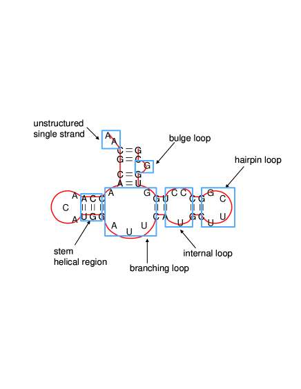
Figure 1: DNA/RNA secondary structure model (reprinted from [9]).

Determining the exact pairings in a secondary structure of a DNA sequence is a complicated task, as we shall try to explain briefly. For a system of interacting entities, one measure commonly used for assessing the system’s property is the free energy. The stability and form of a secondary configuration is usually governed by this energy, the general rule-of-thumb being that a secondary structure minimizes the free energy associated with a DNA sequence. The free energy of a secondary structure is determined by the energy of its constituent pairings. Now, the energy of a pairing depends on the bases involved in the pairing as well as all bases adjacent to it. Adding complication is the fact that in the presence of other neighboring pairings, these energies change according to some nontrivial rules.

Nevertheless, some simple dynamic programming techniques can be used to approximately determine the secondary structure of a DNA sequence. Such approximations usually have the correct form in $70\%$ of the cases considered. Among these techniques, Nussinov’s folding algorithm is the most widely used scheme [10]. Nussinov’s algorithm is based on the assumption that in a DNA sequence $c_{1}c_{2}\ldots c_{n}$, the energy between a pair of bases, $\alpha(c_{i},c_{j})$, is independent of all other pairs. For simplicity of exposition, we shall assume that $\alpha(c_{i},c_{j})=-1$ if $\{{c_{i},c_{j}\}}=\{{\textbf{A},\textbf{T}\}}$, $\alpha(c_{i},c_{j})=-2$ if $\{{c_{i},c_{j}\}}=\{{\textbf{G},\textbf{C}\}}$, and $\alpha(c_{i},c_{j})=0$ otherwise. Let $E_{i,j}$ denote the minimum free energy of the subsequence $c_{i},\ldots,c_{j}$. The independence assumption allows us to compute the minimum free energy of the sequence $c_{1},c_{2},\ldots,c_{n}$ through the recursion

$$E_{i,j}=\min\left\{\begin{array}[]{cc}E_{i+1,j-1}+\alpha(c_{i},c_{j}),&\\ E_{i,k-1}+E_{k,j},&i<k\leq j,\\ \end{array}\right.$$ (2)

where $E_{i,i}=0$ for $i=1,2,...,n$ and $E_{i,i-1}=0$ for $i=2,...,n$. The value of $E_{1,n}$ is the minimum free energy of a secondary structure of $c_{1},c_{2},...,c_{n}$. Note that $E_{1,n}\leq 0$. A very large negative value for the free energy $E_{1,n}$ of a sequence is a good indicator of the presence of stacked base pairs and loops, i.e., a secondary structure, in the physical DNA sequence.

Nussinov’s algorithm can be described in terms of free-energy tables, two of which are shown below. We first describe how such a table is filled out, after which we will point out some important properties of such tables.

	G	C	G	C	C	C	C	G	C
G	0	-2	-2	-4	-4	-4	-4	-6	-6
C	0	0	-2	-2	-2	-2	-2	-4	-4
G	*	0	0	-2	-2	-2	-2	-4	-4
C	*	*	0	0	0	0	0	-2	-2
C	*	*	*	0	0	0	0	-2	-2
C	*	*	*	*	0	0	0	-2	-2
C	*	*	*	*	*	0	0	-2	-2
G	*	*	*	*	*	*	0	0	-2
C	*	*	*	*	*	*	*	0	0

TABLE I: Free-energy table for the sequence GCGCCCCGC

	G	A	G	G	G	T	T	T	T
G	0	0	0	0	0	-1	-1	-1	-1
A	0	0	0	0	0	-1	-1	-1	-1
G	*	0	0	0	0	0	0	0	0
G	*	*	0	0	0	0	0	0	0
G	*	*	*	0	0	0	0	0	0
T	*	*	*	*	0	0	0	0	0
T	*	*	*	*	*	0	0	0	0
T	*	*	*	*	*	*	0	0	0
T	*	*	*	*	*	*	*	0	0

TABLE II: Free-energy table for the sequence GAGGGTTTT

In a free-energy table, the entry at position $(i,j)$ (the top left position being (1,1)), contains the value of $E_{i,j}$. The table is filled out by initializing the entries on the main diagonal and on the first lower sub-diagonal of the matrix to zero, and calculating the energy levels according to the recursion in (2). The calculations proceed successively through the upper diagonals: entries at positions $(1,2),(2,3),...,(n-1,n)$ are calculated first, followed by entries at positions $(1,3),(2,4),...,(n-2,n)$, and so on. Note that the entry at $(i,j),j>i$, depends on $\alpha(i,j)$ and the entries at $(i,l)$, $l=i,\ldots,j-1$, $(l,j)$, $l=i+1,\ldots,n-1$, and $(i+1,j-1)$.

The minimum-energy secondary structure itself can be found by the backtracking algorithm [10] which retraces the steps of Nussinov’s algorithm. The secondary structures for the sequences in Tables I and II, shown in Figures 2 and 3, have been found using the Vienna RNA/DNA secondary structure package [12], which is based on the Nussinov algorithm, but which uses more accurate values for the parameters $\alpha(c_{i},c_{j})$, as well as more sophisticated prediction methods for base pairing probabilities.

Tables I and II show that the minimum free energy for the sequence GCGCCCCGC is $-6$, while that for the sequence GAGGGTTTT is $-1$. This fact alone indicates that the number of paired bases in the first sequence ought to be larger than in the second one, and hence the former is more likely to have a secondary structure than the latter.

More generally, one can observe the following characteristics of free-energy tables: if the first upper diagonal contains a large number of $-1$ or $-2$ entries, then some of these entries “percolate” through to the second upper diagonal, where they get possibly increased by $-1$ or $-2$ if complementary base pairs are present at positions $i$ and $i+2$, $1\leq i\leq n-2$ in the DNA sequence. The values on the second diagonal, in turn, percolate through to the third diagonal, and so on. Hence, the free energy of the DNA sequence depends strongly on the number of non-zero values present on the first diagonal. This phenomenon was also observed experimentally in [2], where the free energy was modelled by a function of the form

$$E_{1,n}=\kappa+\sum_{i=1}^{n-1}\,\alpha(c_{i},c_{i+1}),$$ (3)

with $\kappa$ denoting a correction factor which depends on the number of $G$ and $C$ bases in the sequence c. The stability of a secondary structure, as well as its melting properties can be directly inferred from (3). Note that under the assumption that $\alpha\equiv-1$ for all pairings, the absolute value of the sum in (3) is simply the total number of pairings of complementary bases between the DNA codeword c and the codeword shifted one position to the right or equivalently, the sum of the entries in the first upper diagonal of the free-energy table. These observations imply that a more accurate model for the free energy should be of the form

$$E_{1,n}=\kappa+\gamma_{1}\sum_{i=1}^{n-1}\,\alpha(c_{i},c_{i+1})$$

$$\ \ \ \ \ \mbox{}+\gamma_{2}\sum_{i=1}^{n-2}\,\alpha(c_{i},c_{i+2})+\cdots+\gamma_{l}\sum_{i=1}^{n-l}\,\alpha(c_{i},c_{i+l}),$$

for a correction factor $\kappa$ and some non-zero weighting factors $\gamma_{1}\geq\gamma_{2}\geq\ldots\geq\gamma_{l}$. Furthermore, the same observation implies that from the stand-point of designing DNA codewords without secondary structure, it is desirable to have codewords for which the respective sums of the elements on the first several diagonals are either all zero or of some very small absolute value. This requirement can be rephrased in terms of requiring a DNA sequence to satisfy a shift property, in which a sequence and its first few shifts have few or no complementary base pairs at the same positions.

Figure 2: Secondary structure of the sequence GCGCCCCGC.

Figure 3: Absence of secondary structure in the sequence GAGGGTTTT.

III DNA codewords satisfying a shift property

In this section, we consider the enumeration and construction of DNA sequences satisfying certain shift properties, which we shall define rigorously.

III-A Sequence Enumeration

Definition III.1

The Watson-Crick (WC) distance between two DNA sequences $\mathbf{p}=q_{1}q_{2}\ldots q_{n}$ and $\mathbf{q}=p_{1}p_{2}\ldots p_{n}$ is defined as

$$d_{WC}(\mathbf{p},\mathbf{q})=|\{i:p_{i}\neq\overline{q_{i}}\}|,$$ (4)

i.e., $d_{WC}(\textbf{p},\textbf{q})=d_{H}(\textbf{p},\overline{\textbf{q}})$, where $d_{H}$ stands for the standard Hamming distance.

Given a DNA codeword q, we shall denote by $\textbf{q}_{[i,j]}$, $1\leq i<j\leq n$, the subsequence $q_{i}q_{i+1}\ldots q_{j}$. For $0\leq i\leq n-1$, we define

$$\mu_{i}(\textbf{q})=n-i-d_{WC}(\textbf{q}_{[i+1,n]},\textbf{q}_{[1,n-i]}).$$ (5)

In other words, $\mu_{i}(\textbf{q})$ is the number of indices $\ell\in\{1,2,\ldots,n-i\}$ such that $q_{\ell}=\overline{q_{i+\ell}}$. A shift property of q is now simply any sort of restriction imposed on $\mu_{i}(\textbf{q})$.

Given $s\geq 1$, let $g_{s}(n)$ denote the number of sequences, q, of length $n$ for which $\mu_{i}(\textbf{q})=0$, $i=1,...,s.$ For $n\leq s$, we take $g_{s}(n)$ to be $g_{n-1}(n)$.

Lemma III.1

For all $n>1$, $g_{n-1}(n)=4(2^{n}-1)$.

Proof:

It is clear that a DNA sequence is counted by $g_{n-1}(n)$ iff it contains no pair of complementary bases. Such a sequence must be over one of the alphabets $\{\textbf{A},\textbf{G}\}$, $\{\textbf{A},\textbf{C}\}$, $\{\textbf{T},\textbf{G}\}$ and $\{\textbf{T},\textbf{C}\}$. There are $4(2^{n}-1)$ such sequences, since there are $2^{n}$ sequences over each of these alphabets, of which $\textbf{A}^{n}$, $\textbf{T}^{n}$, $\textbf{G}^{n}$ and $\textbf{C}^{n}$ are each counted twice. ∎

Lemma III.2

For all $n>s$,

$$g_{s}(n)=2g_{s}(n-1)+g_{s}(n-s).$$

Proof:

Let ${\cal G}_{s}(n)$ denote the set of all sequences q of length $n$ for which $\mu_{i}(\textbf{q})=0$, $i=1,...,s$. Thus, $|{\cal G}_{s}(n)|=g_{s}(n)$. Note that for any $\textbf{q}\in{\cal G}_{s}(n)$, $\textbf{q}_{[n-s,n]}$ cannot contain a complementary pair of bases, and hence cannot contain three distinct bases. Let ${\cal E}(n)$ denote the set of sequences $q_{1}...q_{n}\in{\cal G}_{s}(n)$ such that $q_{n-s+1}=q_{n-s+2}=\cdots=q_{n}$, and let ${\cal U}(n)={\cal G}_{s}(n)\setminus{\cal E}(n)$. We thus have $|{\cal E}(n)|+|{\cal U}(n)|=g_{s}(n)$. Each sequence in ${\cal E}(n)$ is obtained from some sequence $q_{1}...q_{n-s+1}\in{\cal G}_{s}(n-s+1)$ by appending $s-1$ bases, $q_{n-s+2},\ldots,q_{n}$, all equal to $q_{n-s+1}$. Hence, $|{\cal E}(n)|=|{\cal G}_{s}(n-s+1)|=g_{s}(n-s+1)$, and therefore, $|{\cal U}(n)|=g_{s}(n)-g_{s}(n-s+1)$.

Now, observe that each sequence $q_{1}q_{2}\ldots q_{n}\in{\cal G}_{s}(n)$ is obtained by appending a single base, $q_{n}$, to some sequence $q_{1}q_{2}\ldots q_{n-1}\in{\cal G}_{s}(n-1)$. If $q_{1}q_{2}\ldots q_{n-1}$ is in fact in ${\cal E}(n-1)$, then there are three choices for $q_{n}$. Otherwise, if $q_{1}q_{2}\ldots q_{n-1}\in{\cal U}(n-1)$, there are only two possible choices for $q_{n}$. Hence,

$$g_{s}(n) = 3\,|{\cal E}(n-1)|+2\,|{\cal U}(n-1)|$$

$$= 3\,g_{s}(n-s)+2\left(g_{s}(n-1)-g_{s}(n-s)\right)$$

This proves the claimed result. ∎

From Lemmas III.1 and III.2, we obtain the following result.

Theorem III.3

The generating function $G_{s}(z)=\sum_{z=1}^{\infty}g_{s}(n)z^{-n}$ is given by

$$G_{s}(z)=4\cdot\frac{z^{s-1}+z^{z-2}+\cdots+z+1}{z^{s}-2z^{s-1}-1}.$$

It can be shown that for $s>1$, the polynomial $\psi_{s}(z)=z^{s}-2z^{s-1}-1$ in the denominator of $G_{s}(z)$ has a real root, $\rho_{s}$, in the interval (2,3), and $s-1$ other roots within the unit circle. It follows that $g_{s}(n)\sim\beta_{s}(\rho_{s})^{n}$ for some constant $\beta_{s}>0$. It is easily seen that $\rho_{s}$ decreases as $s$ increases, and that $\lim_{s\rightarrow\infty}\rho_{s}=2$.

Theorem III.4

The number of length-$n$ DNA sequences q such that $\mu_{1}(\textbf{q})=m$, is $4\binom{n-1}{m}3^{n-m-1}$.

Proof:

Let $B(n,m)$ be the set of length-$n$ DNA sequences q such that $\mu_{1}(\textbf{q})=m$. A sequence $\textbf{q}=q_{1}q_{2}\ldots q_{n}$ is in $B(n,m)$ iff the set $I=\{i:q_{i}=\overline{q_{i-1}}\}$ has cardinality $m$. So, to construct such a sequence, we first arbitrarily pick a $q_{1}$ and an $I\subset\{2,3,\ldots,n\}$, $|I|=m$, which can be done in $4\binom{n-1}{m}$ ways. The rest of q is constructed recursively: for $i\geq 2$, set $q_{i}=\overline{q_{i-1}}$ if $i\in I$, and pick a $q_{i}\neq\overline{q_{i-1}}$ if $i\notin I$. Thus, there are 3 choices for each $i\geq 2$, $i\notin I$, and hence a total of $4\binom{n-1}{m}3^{n-m-1}$ sequences q in $B(n,m)$. ∎

The enumeration of DNA sequences satisfying any sort of shift property becomes considerably more difficult if we bring in the additional requirement of constant GC-content.

Definition III.2

The GC-content, $w_{GC}(\textbf{q})$, of a DNA sequence $\textbf{q}=q_{1}q_{2}\ldots q_{n}$ is defined to be the number of indices $i$ such that $q_{i}\in\{\textbf{G},\textbf{C}\}$.

A DNA code in which all codewords have the same GC-content, $w$, is called a constant GC-content code. The constant GC-content constraint is introduced in order to achieve parallelized operations on DNA sequences, by assuring similar thermodynamic characteristics of all codewords. The GC-content usually needs to be in the range of $30-50\%$ of the length of the code.

The following result can be proved by applying the powerful Goulden-Jackson method of combinatorial enumeration [4, Section 2.8].

Theorem III.5

The number of DNA sequences q of length $n$ and GC-content $w$, such that $\mu_{1}(\textbf{q})=0$, is given by the coefficient of $x^{n}y^{w}$ in the (formal) power series expansion of

$$\Phi(x,y)={\left(1-\frac{2x}{1+x}-\frac{2xy}{1+xy}\right)}^{-1}.$$

III-B Code Construction

The problem of constructing DNA codewords obeying some form of a shift constraint can be reduced to a binary code design problem by mapping the DNA alphabet onto the set of length-two binary words as follows:

$$\textbf{A}\to 00,\;\;\textbf{T}\to 01,\;\;\textbf{C}\to 10,\;\;\textbf{G}\to 11.$$ (6)

Let q be a DNA sequence. The sequence $b$(q) obtained by applying coordinatewise the mapping given in (6) to q will be called the binary image of q. If $b({\mathbf{q}})=b_{0}b_{1}b_{2}\ldots b_{2n-1}$, then the subsequence $e({\mathbf{q}})=b_{0}b_{2}\ldots b_{2n-2}$ will be referred to as the even subsequence of $b(\textbf{q})$, and $o({\mathbf{q}})=b_{1}b_{3}\ldots b_{2n-1}$ will be called the odd subsequence of $b$(q).

The WC distance, $d_{WC}({\mathbf{p}},{\mathbf{r}})$, between two DNA words ${\mathbf{p}},{\mathbf{r}}$ can be expressed in terms of the even and odd subsequences, as stated in the lemma below. For notational ease, given binary words ${\mathbf{x}}=(x_{i})$ and ${\mathbf{y}}=(y_{i})$, we define ${\mathbf{x}}\oplus{\mathbf{y}}=(x_{i}+y_{i})$, the sum being taken modulo-2, and ${\mathbf{x}}*{\mathbf{y}}=(x_{i}y_{i})$.

Lemma III.6

Let p and r be two words of length $n$ over the alphabet $Q$, and define $\sigma_{e}=e({\mathbf{p}})\oplus e({\mathbf{r}})$, $\sigma_{o}=o({\mathbf{p}})\oplus o({\mathbf{r}})$. Using $\overline{{\mathbf{x}}}$ to denote the complement of a binary sequence ${\mathbf{x}}$, we can express the WC distance between ${\mathbf{p}}$ and ${\mathbf{r}}$ as

$$d_{WC}({\mathbf{p}},{\mathbf{r}})=n-w_{H}(\overline{\sigma_{e}}*\sigma_{o})$$

where $w_{H}(\cdot)$ denotes Hamming weight. Consequently, if for some length-$n$ DNA sequence ${\mathbf{q}}$, we take ${\mathbf{p}}={\mathbf{q}}_{[1,n-i]}$ and ${\mathbf{r}}=\textbf{q}_{[i+1,n]}$, then ${\mathbf{q}}$ satisfies the $i$-th shift constraint $\mu_{i}({\mathbf{q}})=0$ iff

$$w_{H}(\overline{\sigma}_{e}*\sigma_{o})=0.$$ (7)

In a companion paper [8], we described a sample of construction methods for DNA codes which reduce undesired hybridization and alow for fully parallel DNA system operation. Among the constraints identified for this problem are the base runlength constraint, the constant GC-content constraint, and the Hamming and reverse-complement Hamming distance constraint. We will show next that it is straightforward to incorporate these hybridization constraints into a scheme which also allows for constructing sequences with reduced probability of secondary structure formation. The idea is based on the use of the non-zero codewords of cyclic simplex codes [5, Chapter 8] or subsets thereof. Recall that a cyclic simplex code of dimension $m$ is a simplex code of length $n=2^{m}-1$ composed of the all-zeros codeword and the $n$ distinct cyclic shifts of any non-zero codeword.

Theorem III.7

Let $\mathcal{C}$ be a DNA code obtained by choosing the set of non-zero codewords of a cyclic simplex code of length $n=2^{m}-1$ for both the even and odd binary code component. Such a code contains $(2^{m}-1)^{2}$ codewords with the property that for all $i\in\{1,2,\ldots,n-1\}$ and $\textbf{q}\in{\cal C}$,

$$\mu_{i}(\textbf{q})\leq 2^{m-2}.$$

Proof:

It is straightforward to see that for any ${\mathbf{q}}\in{\cal C}$, if we let ${\mathbf{p}}={\mathbf{q}}_{[1,n-i]}$, ${\mathbf{r}}={\mathbf{q}}_{[i+1,n]}$, then $\sigma_{e}$ and $\sigma_{o}$, defined as in Lemma 7, are just truncations of codewords from the simplex code. Since the simplex code is a constant-weight code, with minimum distance $2^{m-2}$, each pair of codewords intersects in exactly $2^{m-2}$ positions. This implies that there exist exactly $2^{m-2}$ positions for which one given codeword contains all zeros, and the other codeword contains all ones. These are the positions that are counted in $w_{H}(\overline{\sigma}_{e},\sigma_{o})$, which proves the claimed result. ∎

Example III.8

Consider the previous construction for $m=3$, and a generating codeword $1110100$. There are $49$ DNA codewords of length $7$ obtained based on the outlined method. These codewords have minimum Hamming distance equal to four, and they also have constant $GC$ content $w=4$. A selected subset of codewords from this code is listed below.

$$\begin{split}&\textbf{T}\textbf{G}\textbf{G}\textbf{C}\textbf{T}\textbf{C}\textbf{A},\;\textbf{T}\textbf{C}\textbf{C}\textbf{G}\textbf{T}\textbf{G}\textbf{A},\;\;\textbf{C}\textbf{A}\textbf{C}\textbf{G}\textbf{G}\textbf{T}\textbf{C},\;\textbf{T}\textbf{A}\textbf{G}\textbf{C}\textbf{C}\textbf{T}\textbf{G},\\ &\textbf{C}\textbf{A}\textbf{T}\textbf{G}\textbf{G}\textbf{C}\textbf{T},\;\textbf{G}\textbf{A}\textbf{T}\textbf{C}\textbf{C}\textbf{G}\textbf{T},\;\;\textbf{G}\textbf{G}\textbf{G}\textbf{A}\textbf{G}\textbf{A}\textbf{A},\;\textbf{G}\textbf{G}\textbf{A}\textbf{G}\textbf{A}\textbf{A}\textbf{G}.\end{split}$$

The last two codewords consist of the bases G  and A  only, and clearly satisfy the shift property with $\mu_{i}=0$ for all $i\leq 7$. On the other hand, for the first three codewords one has $\mu_{1}=1$, while for the next three codewords it holds that $\mu_{1}=2$ (meeting the upper bound in the theorem). Due to the cyclic nature of the generating code, one can easily generate the Nussinov folding table for all the codewords [8]. Such an evaluation, as well as the use of the program package Vienna, show that none of the $49$ codewords exhibits a secondary structure. The largest known DNA codes with the parameters specified above consists of $72$ codewords [3]. This code is generated by a simulated annealing process which does not allow for simple secondary structure testing.

References

- [1] L.M. Adleman, “Molecular Computation of Solutions to Combinatorial Problems,” Science, vol. 266, pp. 1021–1024, Nov. 1994.
- [2] K. Breslauer, R. Frank, H. Blocker, and L. Marky, “Predicting DNA Duplex Stability from the Base Sequence,” Proceedings of the National Academy of Science, USA 83, pp. 3746–3750, 1986.
- [3] P. Gaborit, and H. King, “Linear constructions for DNA codes,” preprint.
- [4] I.P. Goulden and D.M. Jackson, Combinatorial Enumeration, Dover, 2004.
- [5] J.I. Hall, Lecture notes on error-control coding, available online at http://www.mth.msu.edu/jhall/.
- [6] F.J. MacWilliams, and N.J.A. Sloane, The Theory of Error Correcting Codes, North-Holland, 1977.
- [7] M. Mansuripur, P.K. Khulbe, S.M. Kuebler, J.W. Perry, M.S. Giridhar and N. Peyghambarian, “Information Storage and Retrieval using Macromolecules as Storage Media,” University of Arizona Technical Report, 2003.
- [8] O. Milenkovic and N. Kashyap, “New Constructions of Codes for DNA Computing,” accepted for presentation at WCC 2005, Bergen, Norway.
- [9] S. Mneimneh, “Computational Biology Lecture 20: RNA secondary structures,” available online at engr.smu.edu/saad/courses/ cse8354/lectures/lecture20.pdf.
- [10] R. Nussinov, G. Pieczenik, J.R. Griggs and D.J. Kleitman, “Algorithms for loop matchings,” SIAM J. Appl. Math., vol. 35, no. 1, pp. 68–82, 1978.
- [11] S. Tsaftaris, A. Katsaggelos, T. Pappas and E. Papoutsakis, “DNA Computing from a Signal Processing Viewpoint,” IEEE Signal Processing Magazine, pp. 100–106, Sept. 2004.
- [12] The Vienna RNA Secondary Structure Package, http://rna.tbi.univie.ac.at/cgi-bin/RNAfold.cgi.