Characterizations of pseudo-codewords
of LDPC codes

Abstract.

An important property of high-performance, low complexity codes is the existence of highly efficient algorithms for their decoding. Many of the most efficient, recent graph-based algorithms, e.g. message passing algorithms and decoding based on linear programming, crucially depend on the efficient representation of a code in a graphical model. In order to understand the performance of these algorithms, we argue for the characterization of codes in terms of a so called fundamental cone in Euclidean space which is a function of a given parity check matrix of a code, rather than of the code itself. We give a number of properties of this fundamental cone derived from its connection to unramified covers of the graphical models on which the decoding algorithms operate. For the class of cycle codes, these developments naturally lead to a characterization of the fundamental polytope as the Newton polytope of the Hashimoto edge zeta function of the underlying graph.

1. Introduction and Background

Whenever information is transmitted across a channel, we have to ensure its integrity against errors. While data may originate in a multitude of applications, at some core level of the communication system, it is usually encoded as a string of zeros and ones of fixed length. Protection against transmission errors is provided by intelligently adding redundant bits to the information symbols, thus effectively restricting the set of possibly transmitted sequences of bits to a fraction of all possible sequences. The set of all possibly transmitted data vectors is called a code, and the elements are called codewords. A classical measure of goodness of a code is the code’s minimum Hamming distance, i.e., the minimum number of coordinates in which any two distinct codewords differ. In fact, a large part of traditional coding theory is concerned with finding the fundamental trade-offs between three parameters: the length of the code, the number of codewords in the code, and the minimum distance of the code.

It is well-known that the minimum Hamming distance $d$ of a code reflects its guaranteed error-correcting capability in the sense that any error pattern of weight at most $\lfloor\frac{d-1}{2}\rfloor$ can be corrected. However, most codes can, with high probability, correct error patterns of substantially higher weight. This insight is the cornerstone of modern coding theory which attempts to capitalize on the full correction capability of a code. One of the most successful realizations of this phenomenon is found in binary low-density parity-check (LDPC) codes. These codes come equipped with an iterative message-passing algorithm to be performed at the receiver’s end which is extremely efficient and corrects, with high probability, many more error patterns than guaranteed by the minimum distance.

In this situation, we are left with the problem of finding new mathematically precise concepts that can take over the role of minimum Hamming distance for such high performance codes. One of the main contributions of this paper is the identification of such a concept, namely, the fundamental cone [6] of a code. Interestingly, the same cone appears when one is considering low-complexity decoding approaches based on solving relaxations of linear programs for maximum-likelihood decoding [2]. We give here a brief motivation of the concept.

As a binary linear code, an LDPC code $C$ is defined by a parity-check matrix $H$. The strength of the iterative decoding algorithm, i.e., its low complexity, comes from the fact that the algorithm operates locally on a so-called Tanner graph representing the matrix $H$. However, this same fact also leads to a fundamental weakness of the algorithm: because it acts locally, the algorithm cannot distinguish if it is acting on the graph itself or on some finite unramified cover of the graph. This leads to the notion of pseudo-codewords, which arise from codewords in codes corresponding to the covers and which compromise the decoder. Thus to understand the performance of LDPC codes, we must understand the graph covers and the codes corresponding to them. As will be seen later in the paper, this is tantamount to understanding a cone in $\mathbb{R}^{n}$ defined by inequalities arising from $H$, called the fundamental cone. We show that the pseudo-codewords of $C$ (with respect to $H$ and the associated Tanner graph) are precisely the integral points in the cone which, modulo 2, reduce to the codewords of $C$.

We emphasize below a few properties of the fundamental cone which appear to be central to a crisp mathematical characterization. A recurring theme is that these properties depend upon the representation of the code as the kernel of a given parity-check matrix, and not solely upon the code itself as a vector space. This showcases the modern viewpoint of coding theory: whereas, classically, the quality of a code was measured in terms of properties (e.g., length, dimension, minimum distance) of the collection of codewords comprising the code, the quality of a code is now measured in terms of properties (e.g., existence of pseudo-codewords of small weight) of a particular representation of the code. Thus, from the modern, algorithmic point of view, a given collection of codewords might be described by two different parity check matrices, one of which might be considered to be very good while another would be very bad.

• The fundamental cone depends on the representation chosen for the code in terms of a parity-check matrix. Note that a linear code has many different parity-check matrices and hence many different cones. This reflects the property of message-passing algorithms that both the complexity and the performance are functions of the structure and, in particular, the sparsity of the parity-check matrix.

• The fundamental cone is an essentially geometric concept relating only to the parity-check matrix and independent of the channel on which the code is employed. Thus we can study codes and their parity-check matrices independently of a specific application.

• The fundamental cone has close ties with well-established mathematical objects. If the parity-check matrix is chosen to be the (highly redundant) matrix containing all words in the dual of the given code, it is readily identified as the metric cone of a binary matroid [1, ch.27], and it is well-studied in this special case. Furthermore, for the particular class of LDPC codes called cycle codes, it is shown in [5] that the fundamental cone is identified with the Newton polyhedron of Hashimoto’s edge zeta function [4] of the normal graph associated to the Tanner graph of the code.

The last bullet above implies that the pseudo-codewords of a cycle code can be read off from the monomials occurring in the power series expansion of the associated zeta function. This gives another characterization of the pseudo-codewords for cycle codes. Inspired by this result, we draw an analogous connection between the pseudo-codewords of a general LDPC code (with respect to a given parity-check matrix), and the monomials of a certain type occurring in the power series expansion of the edge zeta function of the associated Tanner graph.

In summary, we believe that the here-begun study of codes from the perspective of their efficient representation, as reflected in the fundamental polytope, holds the key to a thorough understanding of high performance codes and message-passing decoding algorithms.

The remainder of this paper is organized as follows. In Section 2, we give background on LDPC codes and pseudo-codewords. Section 3 provides a technical yet crucial result about graph covers and their associated matrices. A characterization of pseudo-codewords in the general case via the fundamental cone is given in Section  4. In Section 5 we restrict our attention to the special case of cycle codes and draw the connection to Hashimoto’s edge zeta function. We return to the general case in Section 6, where we show that every LDPC code can be realized as a punctured subcode of a code of the type considered in the previous section. Using the results of Section 5, we then characterize the pseudo-codewords in the general case.

2. Low-Density Parity-Check Codes

We begin with a definition.

Definition 2.1.

Any subspace $C$ of $\mathbb{F}_{2}^{n}$ is called a binary linear code of length $n$. If $C$ is described as the null space of some matrix $H$, i.e.,

$$C=\left\{\mathbf{c}\in\mathbb{F}_{2}^{n}\,\big{|}\,H\mathbf{c}^{\mathsf{T}}=\mathbf{0}\right\},$$

then $H$ is called a parity-check matrix for $C$. If $H$ is sparse, we call $C$ a low-density parity-check (LDPC) code.

Notice that the columns of $H$ correspond to the coordinates, i.e., bits, of the codewords of $C$, and the rows of $H$ give relations, i.e., checks, that these coordinates must satisfy. Although every code has many parity-check matrices, we will always fix a parity-check matrix $H$ for each code we discuss.

The iterative decoding algorithms mentioned in Section 1 operate on a bipartite graph, called the Tanner graph, associated to the matrix $H$.

Definition 2.2.

An undirected graph $G=(V,E)$ consists of a set $V$ of vertices and a collection $E$ of 2-subsets of $V$ called edges. We say $G$ has multiple edges if some 2-subset $\{v,w\}$ of $V$ appears in $E$ at least twice. We say two vertices $v,w\in V$ are adjacent if the set $\{v,w\}$ is an edge. In this case, we say the edge $\{v,w\}$ is incident to both $v$ and $w$. For $v\in V$, we write $\partial(v)$ for the neighborhood of $v$, i.e., the collection of vertices of $G$ which are adjacent to $v$. A bipartite graph with partitions $A$ and $B$ is an undirected graph $G=(V,E)$ such that $V$ can be written as a disjoint union $V=A\cup B$ with no two vertices in $A$ (resp., $B$) adjacent.

We make the following conventions: Unless otherwise specified, our graphs will always be undirected and our bipartite graphs will never have multiple edges.

Definition 2.3.

Let $C\subseteq\mathbb{F}_{2}^{n}$ be the LDPC code determined by the (sparse) $r\times n$ matrix $H=(h_{ji})$. The Tanner graph $T(H)$ is the bipartite graph defined as follows. The vertex set consists of the bit nodes $X=\{x_{1},\dots,x_{n}\}$ and the check nodes $F=\{f_{1},\dots,f_{r}\}$. The set $\{x_{i},f_{j}\}$ is an edge if and only if $h_{ji}=1$.

Notice that the bit nodes in the Tanner graph correspond to the columns of $H$, the check nodes correspond to the rows of $H$, and the edges record which bits are involved in which checks. In other words, the graph $T(H)$ records the matrix $H$, and hence the code $C$, graphically: a binary assignment of the bit nodes $(c_{1},\dots,c_{n})$ is a codeword in $C$ if and only if the binary sum of the values at the neighbors of each check node is zero. Because we have fixed a parity-check matrix $H$ for $C$ from the start, we will also refer to $T=T(H)$ as the Tanner graph of the code $C$.

Example 2.4.

Let $C$ be the binary linear code of length $7$ with parity-check matrix

$$H=\begin{pmatrix}1&1&0&0&0&0&0\\ 0&1&1&1&0&0&0\\ 1&0&1&0&0&0&0\\ 0&0&0&1&1&0&1\\ 0&0&0&0&1&1&0\\ 0&0&0&0&0&1&1\end{pmatrix}.$$

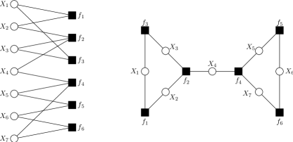
Figure 1. Two representations of the Tanner graph for the code $C$ of Example 2.4.

Two representations of the Tanner graph $T=T(H)$ associated to $H$ are given in Figure 1, where bit and check nodes are represented by empty circles and filled squares, respectively. The graph on the left is a traditional rendering of a bipartite graph, but the one on the right is easier to work with. The vector

$$\mathbf{c}=(c_{1},c_{2},c_{3},c_{4},c_{5},c_{6},c_{7}):=(1,1,1,0,0,0,0)$$

is a codeword in $C$. This can be checked either by computing $H\mathbf{c}^{\mathsf{T}}$ or by assigning the value $c_{i}$ to each bit node $x_{i}$ in $T$ and verifying that the binary sum of the values at the neighbors of each check node $f_{j}$ in $T$ is zero. $\triangle$

Any iterative message-passing decoding algorithm, roughly speaking, operates as follows; see [7] for a more precise description. A received binary word gives an assignment of $0$ or $1$ together with a reliability value at each of the bit nodes on the Tanner graph. Each bit node then broadcasts this bit assignment and reliability value to its neighboring check nodes. Next, each check node makes new estimates based on what it has received from the bit nodes and sends these estimates back to its neighboring bit nodes. By iterating this procedure, one expects a codeword to emerge quickly. Notice that the algorithm is acting locally, i.e., at any stage of the algorithm, the decision made at each vertex is based on information coming only from the neighbors of this vertex. It is this property of the algorithm which causes both its greatest strength (speed) and its greatest weakness (non-optimality). In order to quantify this weakness, we will need another definition.

Definition 2.5.

An unramified, finite cover, or, simply, a cover of a graph $G=(V,E)$ is a graph $\widetilde{G}=(\widetilde{V},\widetilde{E})$ along with a surjection $\pi:\widetilde{V}\to V$ which is a graph homomorphism (i.e., $\pi$ takes adjacent vertices of $\widetilde{G}$ to adjacent vertices of $G$) such that for each vertex $v\in V$ and each $\tilde{v}\in\pi^{-1}(v)$, the neighborhood $\partial(\tilde{v})$ of $\tilde{v}$ is mapped bijectively to $\partial(v)$. A cover is called an $M$-cover, where $M$ is a positive integer, if $\left|\pi^{-1}(v)\right|=M$ for every vertex $v$ in $V$.

Example 2.6.

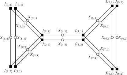
Figure 2. A $2$-cover of the code $C$ from Example 2.4, as described in Example 2.6.

We return to the code $C$ with chosen parity-check matrix $H$ of Example 2.4; the corresponding Tanner graph $T=T(H)$ was given in Figure 1. An example of a 2-cover (or double-cover) $\widetilde{T}$ of $T$ is given in Figure 2. The bipartite graph $\widetilde{T}$ is the Tanner graph for a code $\widetilde{C}$ of length $14=2\cdot 7$.

The parity-check matrix $\widetilde{H}$ for the code $\widetilde{C}$ associated to $\widetilde{T}$ is the $12\times 14$ matrix

$$\widetilde{H}=\begin{pmatrix}I&I&\mathbf{0}&\mathbf{0}&\mathbf{0}&\mathbf{0}&\mathbf{0}\\ \mathbf{0}&J&I&I&\mathbf{0}&\mathbf{0}&\mathbf{0}\\ I&\mathbf{0}&I&\mathbf{0}&\mathbf{0}&\mathbf{0}&\mathbf{0}\\ \mathbf{0}&\mathbf{0}&\mathbf{0}&I&I&\mathbf{0}&J\\ \mathbf{0}&\mathbf{0}&\mathbf{0}&\mathbf{0}&I&I&\mathbf{0}\\ \mathbf{0}&\mathbf{0}&\mathbf{0}&\mathbf{0}&\mathbf{0}&I&I\end{pmatrix},$$

where

$$I=\begin{pmatrix}1&0\\ 0&1\end{pmatrix},\text{\quad}J=\begin{pmatrix}0&1\\ 1&0\end{pmatrix},\text{\quad}\mathbf{0}=\begin{pmatrix}0&0\\ 0&0\end{pmatrix},$$

the rows are ordered to correspond to the check nodes $f_{(1,1)}$, $f_{(1,2)}$, …, $f_{(6,1)}$, $f_{(6,2)}$, and the columns are ordered to correspond to the bit nodes $x_{(1,1)}$, $x_{(1,2)}$, …, $x_{(7,1)}$, $x_{(7,2)}$. $\triangle$

Suppose $T$ is a Tanner graph for the binary linear code $C\subseteq\mathbb{F}_{2}^{n}$ and $\widetilde{T}$ is an $M$-cover of $T$ for some $M\geq 1$. Let $\widetilde{C}\subseteq\mathbb{F}_{2}^{nM}$ be the binary linear code determined by $\widetilde{T}$. To indicate that the coordinates of $\mathbb{F}_{2}^{nM}$ are ordered as in Example 2.6 with each successive block of $M$ coordinates lying above a single coordinate of $\mathbb{F}_{2}^{n}$, we will write an element $\mathbf{x}$ of $\mathbb{F}_{2}^{nM}$ as

$$\mathbf{x}=(x_{(1,1)}{:}\dots:x_{(1,M)},\dots,x_{(n,1)}{:}\dots:x_{(n,M)}).$$

Every codeword in $C$ yields a codeword in $\widetilde{C}$ by “lifting”: if $\mathbf{c}=(c_{1},\dots,c_{n})$ is in $C$, then the vector

$$\hat{\mathbf{c}}=(c_{(1,1)}{:}\dots:c_{(1,M)},\dots,c_{(n,1)}{:}\dots:c_{(n,M)}),$$

where $c_{(i,k)}=c_{i}$ for $1\leq i\leq n$ and $1\leq k\leq M$, is in $\widetilde{C}$. However, there are also codewords in $\widetilde{C}$ which are not liftings of codewords in $C$.

Example 2.7.

Once again, let $C$ be the code of Examples 2.4 and 2.6, and let $\widetilde{C}$ be the code corresponding to the double-cover $\widetilde{T}$ of the Tanner graph $T$ for $C$, as in Example 2.6. The codeword $\mathbf{c}=(1,1,1,0,0,0,0)$ of $C$ lifts to the codeword $\hat{\mathbf{c}}=(1{:}1,1{:}1,1{:}1,0{:}0,0{:}0,0{:}0,0{:}0)$ of $\widetilde{C}$. Although it is easily checked that the vector

$$\tilde{\mathbf{a}}:=(1{:}0,1{:}0,1{:}0,1{:}1,1{:}0,1{:}0,1{:}0)$$

is a codeword in $\widetilde{C}$, it is certainly not a lifting of any codeword in $C$. $\triangle$

Notice that, in general, if

$$\tilde{\mathbf{a}}=(a_{(1,1)}{:}\dots:a_{(1,M)},\dots,a_{(n,1)}{:}\dots:a_{(n,M)})$$

is a codeword in the code corresponding to some $M$-cover $\widetilde{T}$ of $T$, then for any permutations $\sigma_{1}$, …, $\sigma_{n}$ on $\{1,\dots,M\}$, there is an $M$-cover $\widetilde{T}^{\prime}$ of $T$ such that

$$\tilde{\mathbf{a}}^{\prime}=(a_{(1,\sigma_{1}(1))}{:}\dots:a_{(1,\sigma_{1}(M))},\dots,a_{(n,\sigma_{n}(1))}{:}\dots:a_{(n,\sigma_{n}(M))})$$

is a codeword in the code corresponding to $\widetilde{T}^{\prime}$. This motivates the next definition.

Definition 2.8.

Let $C\subseteq\mathbb{F}_{2}^{n}$ be a binary linear code with Tanner graph $T$ and let

$$\tilde{\mathbf{a}}=(a_{(1,1)}{:}\dots:a_{(1,M)},\dots,a_{(n,1)}{:}\dots:a_{(n,M)})$$

be a codeword in the code $\widetilde{C}$ corresponding to some $M$-cover $\widetilde{T}$ of $T$. The unscaled pseudo-codeword corresponding to $\tilde{\mathbf{a}}$ is the vector $\mathbf{p}(\tilde{\mathbf{a}}):=(p_{1},\dots,p_{n})$ where, for $1\leq i\leq n$, $p_{i}$ is the number of nonzero $a_{(i,k)}$, $1\leq k\leq M$. The normalized pseudo-codeword corresponding to $\tilde{\mathbf{a}}$ is the vector $\mbox{\boldmath$\omega$}(\tilde{\mathbf{a}})=(\omega_{1},\dots,\omega_{n})$ where each $\omega_{i}$ is a rational number, $0\leq\omega_{i}\leq 1$, given by $\omega_{i}:=\frac{1}{M}p_{i}$ for $1\leq i\leq M$.

Example 2.9.

The unscaled pseudo-codeword corresponding to the codeword $\tilde{\mathbf{a}}$ on the $2$-cover of Example 2.7 is $(1,1,1,2,1,1,1)$. The corresponding normalized pseudo-codeword is $(\frac{1}{2},\frac{1}{2},\frac{1}{2},1,\frac{1}{2},\frac{1}{2},\frac{1}{2})$. $\triangle$

Notice that if $\mathbf{c}$ is a codeword in our original code and $\hat{\mathbf{c}}$ is the lifting of this codeword to the code corresponding to some finite cover of the Tanner graph, then $\mbox{\boldmath$\omega$}(\hat{\mathbf{c}})=\mathbf{c}$. Indeed, the entries of a normalized pseudo-codeword will be entirely 0’s and 1’s if and only if it comes from the lifting of some actual codeword. Otherwise, there will be at least one entry which is non-integral.

The key issue with graph covers is that locally, any cover of a graph looks exactly like the original graph. Thus, the fact that the iterative message-passing decoding algorithm is operating locally on the Tanner graph $T=T(H)$ means that the algorithm cannot distinguish between the code defined by $T$ and any of the codes defined by finite covers of $T$. This implies that all the codewords in all the covers are competing to be the best explanation of the received vector.

To make this more precise, we assume for simplicity that we are operating on the binary symmetric channel; the situation for other channels is similar (see [6]). Under this assumption, a transmitted bit is received correctly with probability $1-\varepsilon$ and incorrectly with probability $\varepsilon$ where $0\leq\varepsilon<\frac{1}{2}$.

The goal of any decoder is to find the codeword $\mathbf{c}\in C\subseteq\mathbb{F}_{2}^{n}$ that best explains (in some sense) the received vector $\mathbf{y}\in\mathbb{F}_{2}^{n}$. For the binary symmetric channel, a maximum likelihood decoder will find the codeword which is closest in Hamming distance to $\mathbf{y}$. On the other hand, because the iterative decoder of an LDPC code acts locally on the Tanner graph associated to the code, it allows all codewords from all finite covers to compete to be the best explanation of $\mathbf{y}$. In a sense, it automatically lifts $\mathbf{y}$ to vectors $\hat{\mathbf{y}}\in\mathbb{F}_{2}^{nM}$ for every $M\geq 1$ and searches for a codeword $\tilde{\mathbf{a}}$ in some code $\widetilde{C}\subseteq\mathbb{F}_{2}^{nM}$ corresponding to some $M$-cover of the Tanner graph, for some $M\geq 1$, such that $\frac{1}{M}$ times the Hamming distance from (the appropriate) $\hat{\mathbf{y}}$ to $\tilde{\mathbf{a}}$ is minimal among all codewords in all codes corresponding to all finite covers of the Tanner graph. Note that even if fewer than $\lfloor\frac{d-1}{2}\rfloor$ errors have occurred (where $d=d_{\min}(C)$ is the minimum Hamming distance of the code), there may be codewords in covers which are at least as close, in this sense, to $\mathbf{y}$ as is the unique closest codeword.

Example 2.10.

Consider again the code $C$ from Examples 2.4, 2.6, and 2.7. Assume that we are transmitting over a binary symmetric channel and we receive the vector $\mathbf{y}=(1,0,1,1,0,1,0)$.

One can check that the codeword $\mathbf{c}=(1,1,1,0,0,0,0)$ satisfies $d(\mathbf{y},\mathbf{c})=3$ and that the Hamming distance from $\mathbf{y}$ to any other codeword in $C$ is larger than $3$. Therefore, a maximum-likelihood decoder would output the codeword $\mathbf{c}$ when $\mathbf{y}$ is received.

But the iterative message-passing decoding algorithm allows all the codewords in all the codes corresponding to all the finite covers to compete. In particular, the vector $\tilde{\mathbf{a}}=(1{:}0,1{:}0,1{:}0,1{:}1,1{:}0,1{:}0,1{:}0)$ from Example 2.6 lies in the code $\widetilde{C}$ corresponding to the double cover $\widetilde{T}$ of $T$ and is hence a competitor. Letting $\hat{\mathbf{y}}=(1{:}1,0{:}0,1{:}1,1{:}1,0{:}0,1{:}1,0{:}0)$ be the lifting of $\mathbf{y}$ to $\mathbb{F}_{2}^{14}$, we see that $\frac{1}{2}$ times the Hamming distance from $\hat{\mathbf{y}}$ to $\tilde{\mathbf{a}}$ is also 3. Hence $\tilde{\mathbf{a}}$ is just as attractive to the iterative decoder as $\mathbf{c}$ is. The iterative decoder becomes confused. $\triangle$

The situation observed in Example 2.10 happens in general: one can easily exhibit a received vector $\mathbf{y}$ and a codeword $\tilde{\mathbf{a}}$ in an $M$-cover for some $M$ such that $\frac{1}{M}$ times the distance from $\hat{\mathbf{y}}$ to $\tilde{\mathbf{a}}$ is at most $d(\mathbf{y},\mathbf{c})$ for any codeword $\mathbf{c}$ in the original code. As mentioned above, there is nothing special about the binary symmetric channel, and so the above statements can easily be generalized to other channels.

Thus, in order to understand iterative decoding algorithms, it is crucial to understand the codewords in the codes corresponding to all finite covers of $T(H)$. The remainder of this paper is devoted to this task.

3. Liftings

We saw in Section 2 above that understanding finite covers of graphs is crucial to understanding the performance of the iterative decoding algorithm used for LDPC codes. The main result of this section, Theorem 3.3, will help us to reach this goal. Though it is rather technical, the remainder of the paper hinges upon it.

We first state a lemma, the proof of which follows immediately from the definition of an $M$-cover (Definition 2.5).

Lemma 3.1.

Let $H=(h_{ji})$ be the parity-check matrix associated to the Tanner graph $T$ and let $\widetilde{T}$ be an $M$-cover of $T$. Let $\widetilde{H}=(h_{(j,l),(i,k)})$, $1\leq k\leq M$ and $1\leq l\leq M$, be the parity-check matrix associated to $\widetilde{T}$. Then for each $i$ and $j$, there is a permutation $\sigma_{ji}$ on $\{1,\dots,M\}$ such that $h_{(j,l),(i,k)}=1$ if and only if $h_{ji}=1$ and $\sigma_{ji}(l)=k$. Conversely, choosing permutations $\sigma_{ji}$ on $\{1,\dots,M\}$ for all $i$ and $j$ uniquely and completely determines an $M$-cover $\widetilde{T}$ of $T$ and its corresponding parity-check matrix $\widetilde{H}$.

A simple interpretation of Lemma 3.1 is that if $H$ has associated Tanner graph $T$ and $\widetilde{T}$ is an $M$-cover of $T$, then the matrix $\widetilde{H}$ associated to $\widetilde{T}$ can be obtained by replacing each 0 of $H$ with an $M\times M$ matrix of 0’s and each 1 of $H$ with a suitably chosen $M\times M$ permutation matrix. We need one more definition before we can state the main result of this section.

Definition 3.2.

Let $G=(V,E)$ be a graph. Fix an ordering of the edges, so that we have $E=\{e_{1},\dots,e_{n}\}$. A sequence of edges $(e_{i_{1}},\dots,e_{i_{k}})$ of $G$ is a path on $G$ if the edges $e_{i_{j}}$ can be directed so that $e_{i_{s}}$ terminates where $e_{i_{s+1}}$ begins for $1\leq s\leq k-1$. We say the path is backtrackless if for no $s$ do we have $e_{i_{s}}=e_{i_{s+1}}$. We say two paths are edge-disjoint if they do not share an edge.

The next theorem is the main result of this section. It gives conditions under which a collection of edges, with multiplicities, on a graph may be lifted to a union of edge-disjoint paths on some finite cover of the graph. It will be used in Section 4 to show that every vector of nonnegative integers which lies in the fundamental cone and which reduces modulo 2 to a codeword must be a pseudo-codeword, and that result will be used in turn in Section 6 to characterize pseudo-codewords in the case in which all bit nodes in the Tanner graph have even degree. The proof is constructive, providing an algorithm to produce the desired paths.

Theorem 3.3.

Let $T=(X\cup F,E)$ be a bipartite graph. Suppose that to each $e\in E$ there is assigned a nonnegative integer $m_{e}$ such that

1. For each $x\in X$, there is a nonnegative integer $M_{x}$ such that $m_{e}=M_{x}$ for every edge $e$ incident to $x$.

2. For each $f\in F$, the sum $\displaystyle{\sum_{x\in\partial(f)}M_{x}}$ is even.

3. For each $f\in F$ and each $x\in\partial(f)$, we have $\displaystyle{\sum_{y\in\partial(f)\setminus\{x\}}M_{y}\geq M_{x}}$.

Then there is a finite cover $\pi:\widetilde{T}:=(\widetilde{X}\cup\widetilde{F},\widetilde{E})\to T$ and a union $\Delta:=\Delta_{1}\cup\dots\cup\Delta_{p}$ of backtrackless paths $\Delta_{i}$ on $\widetilde{T}$ such that the endpoints of each $\Delta_{i}$ are in $\widetilde{X}$ and such that

1. Each $\tilde{f}\in\widetilde{F}$ occurs in $\Delta$ at most once.

2. Each $\tilde{e}\in\widetilde{E}$ occurs in $\Delta$ at most once.

3. At each $\tilde{x}\in\widetilde{X}$, either all or none of the edges incident to $\tilde{x}$ in $\widetilde{T}$ occur in $\Delta$.

4. For each $e\in E$, we have $\left|\pi^{-1}(e)\cap\Delta\right|=m_{e}$.

Proof.

We will refer to $X$ as the set of bit nodes of $T$ and to $F$ as the set of check nodes of $T$. Let $\Gamma$ be the multiset of edges of $T$ which contains, for each $e\in E$, a total of $m_{e}$ copies of $e$. For each $f\in F$, let $N_{f}$ be the number of edges in $\Gamma$ which are incident to $f$, counted with multiplicity. In other words,

$$N_{f}=\sum_{x\in\partial(f)}M_{x}.$$

Set $M:=\max\left(\{M_{x}\,|\,x\in X\}\cup\{\frac{1}{2}N_{f}\,|\,f\in F\}\right)$. We construct an $M$-cover $\pi:\widetilde{T}\to T$ and the desired $\Delta$ explicitly. The vertex set of $\widetilde{T}$ is

$$\{x_{k}\,|\,x\in X\text{ and }1\leq k\leq M\}\cup\{f_{l}\,|\,f\in F\text{ and }1\leq l\leq M\}$$

and the map $\pi:\widetilde{T}\to T$ is given by $\pi(x_{k})=x$, $\pi(f_{l})=f$. We now need to describe the edges of $\widetilde{T}$ and the disjoint paths $\Delta_{i}$. We will first describe the edges of $\widetilde{T}$ which are involved in the $\Delta_{i}$’s, and then we will describe the remaining edges of $\widetilde{T}$. The bit nodes of $\widetilde{T}$ involved in the $\Delta_{i}$’s are $\{x_{k}\,|\,x\in X\text{ and }1\leq k\leq M_{x}\}$ and the check nodes of $\widetilde{T}$ involved in the $\Delta_{i}$’s are $\{f_{l}\,|\,f\in F\text{ and }1\leq l\leq\frac{1}{2}N_{f}\}$.

Start by writing out, for each $x\in X$, $M_{x}$ copies of the list $\partial(x)$ of neighbors of $x$; label these lists using the bit nodes $x_{1},\dots x_{M_{x}}$ of $\widetilde{T}$ lying above $x$ so that $L(x_{1})\dots,L(x_{M_{x}})$ are the $M_{x}$ copies of $\partial(x)$. Notice that there is a 1-1 correspondence between the edges in $\Gamma$ (with multiplicity) and pairs $(x_{k},f)$ where $f$ occurs in $L(x_{k})$. Similarly, write out, for each $f\in F$, one copy of the list $\partial(f)$ of neighbors of $f$, but then replace each $x$ appearing in the list with the bit nodes $x_{1},\dots,x_{M_{x}}$ of $\widetilde{T}$ so that the list has length $N_{f}$; call this list $L(f)$. Again, we have a 1-1 correspondence between the edges in $\Gamma$ (with multiplicity) and the pairs $(f,x_{k})$, where $x_{k}$ occurs in $L(f)$. We will construct the $\Delta_{i}$’s one vertex at a time. Each time we add a vertex (except for the initial vertex of each $\Delta_{i}$), we are choosing an edge from $\Gamma$ and lifting it to $\widetilde{T}$, and so we will cross one check node off a list labeled by a bit node and one bit node off a list labeled by a check node. Thus the lists $L(x_{k})$ and $L(f)$ change as the algorithm proceeds.

We will need some terminology and notation in the construction:

• At any given point in the algorithm and for any vertex $v$, let the current weight of $v$ be the number of elements in $L(v)$.

• At any given point in the algorithm and for $x\in X$ and $f\in F$, set $m_{f}(x):=\#\{i\,|\,x_{i}\in L(f)\}$.

Notice that since, as mentioned above, the lists $L(v)$ change as the algorithm proceeds, the current weight of a vertex and the value $m_{f}(x)$ for $x\in X$ and $f\in F$ do as well. At the beginning, the current weight of $x_{k}$ ($x\in X$ and $1\leq k\leq M_{x}$) is $|\partial(x)|$, the current weight of $f\in F$ is $N_{f}$, and $m_{f}(x)=M_{x}$ if $f\in\partial(x)$ and $0$ otherwise. To construct the $\Delta_{i}$’s which form $\Delta$, we proceed as follows:

1. Choose a bit node of $\widetilde{T}$ whose current weight is at least that of every other bit node of $\widetilde{T}$ and take it to be the first vertex in a path $P$.

2. Suppose we have just added the bit node $x_{k}$ to $P$, where $x\in X$ and $1\leq k\leq M_{x}$, and that $L(x_{k})\neq\emptyset$. Choose a check node $f\in L(x_{k})$ such that the current weight of $f$ is at least that of any other check node in $L(x_{k})$. Write down $f_{s}$ as the next vertex of $P$, where $s$ is the number of times (including this one) that $f$ has been used so far in all of $\Delta$. Cross $f$ off $L(x_{k})$ and cross $x_{k}$ off $L(f)$.

3. Suppose we have just added the bit node $x_{k}$ and then the check node $f_{s}$ to $P$, where $x\in X$, $f\in F$, $1\leq k\leq M_{x}$, and $1\leq s\leq N_{f}$. Let $L(f)\setminus x$ denote the set of vertices in $L(f)$ which are not of the form $x_{i}$ for any $i$; Claim 1 below shows that $L(f)\setminus x$ is nonempty. Let $y_{l}\in L(f)\setminus x$ be such that $m_{f}(y)\geq m_{f}(w)$ for all $w$ such that $w_{t}\in L(f)\setminus x$ for some $t$ and the current weight of $y_{l}$ is at least that of any other $y_{i}\in L(f)$. Append the vertex $y_{l}$ to $P$. Cross $y_{l}$ off $L(f)$ and $f$ off $L(y_{l})$. If $L(y_{l})$ is now empty, then $P$ is complete and will be one of the $\Delta_{i}$’s in the disjoint union $\Delta$. Otherwise, return to Step (2).

4. If there are nonempty lists remaining, start over with Step (1) on the remaining set of vertices. Otherwise, $\Delta$ is the union of the $\Delta_{i}$’s and the algorithm is complete.

It is now clear from the construction and hypothesis (H.1) that $\Delta=\Delta_{1}\cup\dots\cup\Delta_{p}$ is a union of paths satisfying conditions (C.1), (C.2) and (C.4). Claim 1 below shows that each $\Delta_{i}$ is backtrackless, and hypothesis (H.2) implies that the ending vertices must be bit nodes since the starting vertices are. To see that condition (C.3) holds, let $x\in X$ and consider two cases. If $k>M_{x}$, then $x_{k}$ is not involved in $\Delta$ and so no edge incident to $x_{k}$ occurs in $\Delta$. If $1\leq k\leq M_{x}$, we have $\left|\partial(x)\right|$ edges incident to $x_{k}$ involved in $\Delta$. Since the degree of $x_{k}$ in $\widetilde{T}$ is to be the same as the degree of $x$ in $T$, we have that all edges which are to be incident to $x_{k}$ in $\widetilde{T}$ occur already in $\Delta$.

All that remains is to add additional edges to $\widetilde{T}$ so that $\pi:\widetilde{T}\to T$ is an $M$-cover. In order for $\pi:\widetilde{T}\to T$ to be an $M$-cover of $T$, we must have, for each bit node $x$ of $T$ and each $k$ with $1\leq k\leq M$,

$$|\partial(x_{k})|=|\partial(x)|$$

and

$$\{f\,|\,f_{l}\in\partial(x_{k})\text{ for some }l\}=\partial(x).$$

Let $x\in X$. As mentioned above, these properties hold already for $x_{k}$ with $1\leq k\leq M_{x}$, and we have constructed no edges involving the $M-M_{x}$ other bit nodes $x_{k}$ of $\widetilde{T}$. Similarly, for each check node $f$ with $f\in\partial(x)$, we know that exactly $M_{x}$ of the vertices $f_{t}$ are connected by an edge to some $x_{s}$, which means that there are $M-M_{x}$ vertices $f_{l}$ which are not connected by an edge to any $x_{s}$. We can pair up these $M-M_{x}$ bit nodes $x_{k}$ and these $M-M_{x}$ check nodes $f_{l}$ any way we please. In particular, this will not change any bit nodes already involved in our $\Delta$, and when we are done doing this for each $x$, we will have the $M$-cover $\pi:\widetilde{T}\to T$ and the $\Delta$ we seek.

The proof of Theorem 3.3 will be complete once we have proven Claim 1.

Claim 1.

Steps (2) and (3) can always be performed without introducing a backtrack. In particular, the set $L(f)\setminus x$ in Step (3) of the algorithm is nonempty.

Proof.

For each bit node $w\in X$, let $m_{f}^{\mathrm{s}}(w)$ be the value of $m_{f}(w)$ at the start of Step (2) and let $m_{f}^{\mathrm{e}}(w)$ be the value of $m_{f}(w)$ at the end of Step (3). For each $w\in X$ and each $f\in F$, let $I^{\mathrm{s}}(w,f)$ denote the inequality

$$\sum_{y\in X\setminus\{w\}}m_{f}^{\mathrm{s}}(y)\geq m_{f}^{\mathrm{s}}(w)$$

and let $I^{\mathrm{e}}(w,f)$ denote the inequality

$$\sum_{y\in X\setminus\{w\}}m_{f}^{\mathrm{e}}(y)\geq m_{f}^{\mathrm{e}}(w).$$

Notice that at the start of the algorithm, $I^{\mathrm{s}}(w,f)$ is true for every $w$ and $f$ by hypothesis (H.3).

Suppose $I^{\mathrm{s}}(w,f)$ holds for every $w$ and $f$ and that we are at the start of Step (2), having just appended $x_{k}$ to $P$. We will show that we can perform Steps (2) and (3) without introducing a backtrack, and that the inequalities $I^{\mathrm{e}}(w,f)$ will hold when we are done with these two steps. This will mean that we can continue to perform these steps until we are forced to move on to Step (4).

Since each check node occurs in $L(x_{k})$ at most once, we know that $L(x_{k})$ no longer contains the check node we appended to $\Delta$ just before we appended $x_{k}$. So, since $L(x_{k})$ is, by assumption, nonempty, Step (2) can be performed and it does not introduce a backtrack; let $f$ be the check node appended to $\Delta$ in that step, so that $m_{f}^{\mathrm{e}}(x)=m_{f}^{\mathrm{s}}(x)-1$. Since $I^{\mathrm{s}}(x,f)$ held before Step (2), we know that there is at least one $y\neq x$ such that $y_{i}\in L(f)$ for some $i$, i.e., $L(f)\setminus x$ is nonempty. So Step (3) can be performed, and we have $m_{f}^{\mathrm{e}}(y)=m_{f}^{\mathrm{s}}(y)-1$ for the $y\in X$ chosen in that step. For all other bit nodes $w$, we have $m_{f}^{\mathrm{e}}(w)=m_{f}^{\mathrm{s}}(w)$. We now need to show that the inequality $I^{\mathrm{e}}(w,f)$ holds for every $w\in X$. First note that $I^{\mathrm{e}}(x,f)$ is obtained from $I^{\mathrm{s}}(x,f)$ by subtracting 1 from each side. Since $I^{\mathrm{s}}(x,f)$ held, $I^{\mathrm{e}}(x,f)$ must also. The same argument shows that $I^{\mathrm{e}}(y,f)$ holds. Further, $I^{\mathrm{e}}(w,f)$ holds whenever $m_{f}^{\mathrm{e}}(w)=m_{f}^{\mathrm{s}}(w)=0$ since what appears on the left-hand side of $I^{\mathrm{e}}(w,f)$ is certainly nonnegative. Hence we need only show that $I^{\mathrm{e}}(w,f)$ holds for $w\in X\setminus\{x,y\}$ with $m_{f}^{\mathrm{e}}(w)=m_{f}^{\mathrm{s}}(w)\geq 1$.

So suppose $m_{f}^{\mathrm{e}}(w)=m_{f}^{\mathrm{s}}(w)\geq 1$. Consider first the case where $m_{f}^{\mathrm{e}}(v)=m_{f}^{\mathrm{s}}(v)=0$ for all $v\in X\setminus\{x,y,w\}$. Then the inequality $I^{\mathrm{e}}(w,f)$ says

$$m_{f}^{\mathrm{e}}(x)+m_{f}^{\mathrm{e}}(y)\geq m_{f}^{\mathrm{e}}(w),\text{\qquad i.e., \qquad}m_{f}^{\mathrm{s}}(x)+m_{f}^{\mathrm{s}}(y)-2\geq m_{f}^{\mathrm{s}}(w).$$

If $m_{f}^{\mathrm{s}}(y)=m_{f}^{\mathrm{s}}(w)$, then, since $m_{f}^{\mathrm{s}}(x)+m_{f}^{\mathrm{s}}(y)+m_{f}^{\mathrm{s}}(w)$ is even, we know that $m_{f}^{\mathrm{s}}(x)\geq 2$ and so $I^{\mathrm{e}}(w,f)$ holds. Otherwise, we have $m_{f}^{\mathrm{s}}(y)\geq m_{f}^{\mathrm{s}}(w)+1$ and so, since $m_{f}^{\mathrm{s}}(x)\geq 1$, we again see that $I^{\mathrm{e}}(w,f)$ holds.

Now consider the case that there is at least one bit node $v\in X\setminus\{x,y,w\}$ with $m_{f}^{\mathrm{e}}(v)=m_{f}^{\mathrm{s}}(v)\geq 1$. Then it is enough to show that

$$m_{f}^{\mathrm{e}}(x)+m_{f}^{\mathrm{e}}(y)+m_{f}^{\mathrm{e}}(v)\geq m_{f}^{\mathrm{e}}(w).$$

But this is the same as

$$m_{f}^{\mathrm{s}}(x)+m_{f}^{\mathrm{s}}(y)+m_{f}^{\mathrm{s}}(v)-2\geq m_{f}^{\mathrm{s}}(w).$$

Since $m_{f}^{\mathrm{s}}(y)\geq m_{f}^{\mathrm{s}}(w)$ and each of $m_{f}^{\mathrm{s}}(x)$ and $m_{f}^{\mathrm{s}}(v)$ is at least 1, this latter inequality holds and so $I^{\mathrm{e}}(w,f)$ does as well. ∎

This completes the proof of Theorem 3.3. ∎

4. The Fundamental Cone

The pseudo-codewords are described for general LDPC codes by the fundamental cone.

Definition 4.1.

Let $H=(h_{ji})$ be an $r\times n$ matrix with $h_{ji}\in\{0,1\}$ for each $j$ and $i$. The fundamental cone $\mathcal{K}(H)$ of $H$ is the set of vectors $\mbox{\boldmath$\nu$}=(\nu_{1},\dots,\nu_{n})\in\mathbb{R}^{n}$ such that, for all $1\leq i\leq n$ and $1\leq j\leq r$, we have

(4.1) $$\nu_{i}\geq 0$$

and

(4.2) $$\sum_{i^{\prime}\neq i}h_{ji^{\prime}}\nu_{i^{\prime}}\geq h_{ji}\nu_{i}.$$

Remark 4.2.

The matrices $H$ we consider will be parity-check matrices of binary linear codes. As such, we will sometimes be doing computations over $\mathbb{F}_{2}$ (e.g., when deciding if a vector is a codeword) and sometimes over $\mathbb{R}$ (e.g., when deciding if a vector is in the fundamental cone). Although the field over which we are working should usually be clear from context, we will typically specify it explicitly to help avoid confusion.

Example 4.3.

The fundamental cone $\mathcal{K}(H)$ for the parity-check matrix $H$ of the code $C$ from Example 2.4 is

$$\mathcal{K}(H)=\Bigg{\{}(\nu_{1},\dots,\nu_{7})\in\mathbb{R}^{7}\,\Bigg{|}\,\begin{matrix}\nu_{i}\geq 0\text{ for $1\leq i\leq 7$ }\\ \nu_{1}=\nu_{2}=\nu_{3},\text{\quad}\nu_{5}=\nu_{6}=\nu_{7}\\ 2\nu_{1}\geq\nu_{4},\text{\quad}2\nu_{5}\geq\nu_{4}\end{matrix}\Bigg{\}}.$$

Notice that the unscaled pseudocodeword $(1,1,1,2,1,1,1)$ and the normalized pseudocodeword $(\frac{1}{2},\frac{1}{2},\frac{1}{2},1,\frac{1}{2},\frac{1}{2},\frac{1}{2})$ from Example 2.9 lie in $\mathcal{K}(H)$. $\triangle$

The importance of the fundamental cone is illustrated below by Theorem 4.4, Corollary 4.5 and Theorem 4.6.

Theorem 4.4.

Let $H=(h_{ji})$ be an $r\times n$ matrix with $h_{ji}\in\{0,1\}$ for each $j$ and $i$, $\mathcal{K}=\mathcal{K}(H)$ the fundamental cone of $H$, and $C$ the binary code with parity-check matrix $H$. Let $\mathbf{p}=(p_{1},\dots,p_{n})$ be a vector of integers. Then the following are equivalent:

1. $\mathbf{p}$ is an unscaled pseudo-codeword.

2. $\mathbf{p}\in\mathcal{K}$ and $H\mathbf{p}^{\mathsf{T}}=\mathbf{0}\in\mathbb{F}_{2}^{r}$.

In other words, the unscaled pseudo-codewords are precisely those integer vectors in the fundamental cone which reduce modulo 2 to codewords.

Proof.

Suppose that $\mathbf{p}$ is an unscaled pseudo-codeword. Then there is an $M$-cover $\widetilde{T}$ of the Tanner graph $T$ associated to $H$ and a codeword

$$\tilde{\mathbf{c}}=(c_{(1,1)}{:}\dots:c_{(1,M)},\dots,\ c_{(n,1)}{:}\dots:c_{(n,M)})$$

in $\widetilde{C}$, the code associated to $\widetilde{T}$, such that, for each $i$, exactly $p_{i}$ of the coordinates $c_{(i,k)}$, $1\leq k\leq M$, are 1. Let $\widetilde{H}=(h_{(j,l),(i,k)})$, where $1\leq j\leq r$, $1\leq i\leq n$, $1\leq k\leq M$, and $1\leq l\leq M$, be the parity-check matrix of the code $\widetilde{C}$ associated to $\widetilde{T}$. For each $i$ and $j$, let $\sigma_{ji}$ be as in Lemma 3.1, so that $h_{(j,l),(i,k)}=1$ if and only if $h_{ji}=1$ and $k=\sigma_{ji}(l)$. Then the equation $\widetilde{H}\tilde{\mathbf{c}}^{\mathsf{T}}=\mathbf{0}\in\mathbb{F}_{2}^{rM}$ implies that, in $\mathbb{F}_{2}$, we have for each $j$ and $l$,

(4.3) $$0=\sum_{i=1}^{n}\sum_{k=1}^{M}h_{(j,l),(i,k)}c_{(i,k)}=\sum_{i=1}^{n}h_{ji}c_{(i,\sigma_{ji}(l))}.$$

We shall use this observation to prove that $\mathbf{p}\in\mathcal{K}$ and that $H\mathbf{p}^{\mathsf{T}}=\mathbf{0}\in\mathbb{F}_{2}^{r}$.

We first show that $\mathbf{p}\in\mathcal{K}$. Clearly inequalities (4.1) hold for $\mbox{\boldmath$\nu$}=\mathbf{p}$, and we must show that inequalities (4.2) do as well. Thus, we must show that we have

(4.4) $$\sum_{1\leq k\leq M}\sum_{i^{\prime}\neq i}h_{ji^{\prime}}c_{(i^{\prime},k)}\geq\sum_{1\leq k\leq M}h_{ji}c_{(i,k)}$$

for each $i$ and $j$. Certainly (4.4) holds if $h_{ji}=0$ or if $c_{(i,k)}=0$ for all $k$. So assume $h_{ji}=1$ and not all $c_{(i,k)}$ are zero. For each $k$ with $c_{(i,k)}=1$, set $l_{k}:=\sigma_{ji}^{-1}(k)$. Then we have by (4.3) that the integer sum

$$\sum_{i^{\prime}=1}^{n}h_{ji^{\prime}}c_{(i^{\prime},\sigma_{ji^{\prime}}(l_{k}))}$$

is even. Hence, for each $k$ with $c_{(i,k)}=1$, there is at least one value of $i^{\prime}\neq i$ such that $h_{ji^{\prime}}=c_{(i^{\prime},\sigma_{ji^{\prime}}(l_{k}))}=1$. Note that as $k$ varies, the indices $(i^{\prime},\,\sigma_{ji^{\prime}}(l_{k}))$ are all distinct. Thus (4.4) holds and so $\mathbf{p}\in\mathcal{K}$.

To see that $H\mathbf{p}^{\mathsf{T}}=\mathbf{0}\in\mathbb{F}_{2}^{r}$, sum (4.3) over $l$ to get that for each $j$, we have

$$0=\sum_{l=1}^{M}\sum_{i=1}^{n}h_{ji}c_{(i,\sigma_{ji}(l))}$$

in $\mathbb{F}_{2}$. After interchanging the summations over $l$ and $i$, we may use the fact that $\sigma_{ji}$ is a permutation and substitute the summation variable $l$ by $k=\sigma_{ji}(l)$ to get

$$0=\sum_{i=1}^{n}h_{ji}\sum_{k=1}^{M}c_{(i,k)}=\sum_{i=1}^{n}h_{ji}p_{i}$$

in $\mathbb{F}_{2}$, i.e., $H\mathbf{p}^{\mathsf{T}}=\mathbf{0}\in\mathbb{F}_{2}^{r}$.

Conversely, suppose $\mathbf{p}=(p_{1},\dots,p_{n})\in\mathcal{K}$ and $H\mathbf{p}^{\mathsf{T}}=\mathbf{0}\in\mathbb{F}_{2}^{r}$. Let $T$ be the Tanner graph associated to $H$, and label the bit nodes of $T$ as $x_{1},\dots,x_{n}$ to correspond to the $n$ columns of $H$. For $1\leq i\leq n$, set $M_{x_{i}}=p_{i}$. For each edge $e$ of $T$, there is a unique $i$, $1\leq i\leq n$, such that $e$ is incident to $x_{i}$; set $m_{e}:=p_{i}$ for this value of $i$. Then hypothesis (H.1) of Theorem 3.3 is satisfied. That hypothesis (H.2) is satisfied follows directly from the fact that $H\mathbf{p}^{\mathsf{T}}=\mathbf{0}\in\mathbb{F}_{2}^{r}$. The fact that $\mathbf{p}\in\mathcal{K}$ says that hypothesis (H.3) holds. Thus Theorem 3.3 applies and we have a finite $M$-cover $\widetilde{T}$ of $T$ for some $M\geq 1$ and a union $\Delta:=\Delta_{1}\cup\dots\cup\Delta_{p}$ of backtrackless paths on $\widetilde{T}$ starting and ending at bit nodes of $\widetilde{T}$ and satisfying conditions (C.1)–(C.4) of that theorem. Label the bit nodes of $\widetilde{T}$ as $x_{(i,k)}$ for $1\leq i\leq n$ and $1\leq k\leq M$, and let

$$\tilde{\mathbf{c}}=(c_{(1,1)}{:}\dots:c_{(1,M)},\dots,c_{(n,1)}{:}c_{(n,M)})\in\mathbb{F}_{2}^{nM}$$

be the vector given by the rule $c_{(i,k)}=1$ if and only if $x_{(i,k)}$ occurs in $\Delta$, i.e., if and only if $1\leq k\leq p_{i}$. Then conditions (C.1)–(C.4) ensure that $\tilde{\mathbf{c}}$ is a codeword in the code corresponding to $\widetilde{T}$. Finally, we see that the unscaled pseudo-codeword associated to $\tilde{\mathbf{c}}$ is precisely $\mathbf{p}$. ∎

Corollary 4.5.

Every normalized pseudo-codeword lies in the fundamental cone.

Proof.

Let $\mbox{\boldmath$\omega$}=\frac{1}{M}\mathbf{p}$ be a normalized pseudo-codeword, where $\mathbf{p}$ is an unscaled pseudo-codeword coming from a codeword in the code corresponding to some $M$-cover. Then $\mathbf{p}\in\mathcal{K}$ by Theorem 4.4 and so $\mbox{\boldmath$\omega$}\in\mathcal{K}$ since $\mathcal{K}$ is a cone. ∎

Theorem 4.6.

The rays through the pseudo-codewords are dense in the fundamental cone. More precisely, let $C$ be a binary linear code with parity-check matrix $H$, Tanner graph $T=T(H)$ and fundamental cone $\mathcal{K}=\mathcal{K}(H)$, and let $\mbox{\boldmath$\nu$}\in\mathcal{K}(H)$. Then for any $\varepsilon>0$, there is a pseudo-codeword $\mathbf{p}$ such that $||\alpha\mathbf{p}-\mbox{\boldmath$\nu$}||<\varepsilon$ for some $\alpha>0$.

Proof.

Let $n$ be the length of $C$, so that $\mbox{\boldmath$\nu$}=(\nu_{1},\dots,\nu_{n})\in\mathbb{R}^{n}$. Choose $\beta\in\mathbb{R}$ sufficiently large so that the vector $\mathbf{p}:=\mathbf{p}(\beta)=(p_{1},\dots,p_{n})$, where $p_{i}=2\lceil\beta\nu_{i}\rceil$, satisfies $||\alpha\mathbf{p}-\mbox{\boldmath$\nu$}||<\varepsilon$ for some $\alpha>0$. For example, if $n=1$ we may take $\beta=\frac{1}{\varepsilon}$ and $\alpha=\frac{\varepsilon}{2}$.

We claim $\mathbf{p}\in\mathcal{K}$. Certainly $p_{i}\geq 0$ for $1\leq i\leq n$, and we must show that inequalities (4.2) hold for $\mathbf{p}$. Since $\mbox{\boldmath$\nu$}\in\mathcal{K}(H)$ by assumption, we know that inequalities (4.2) hold for $\nu$. Multiplying both sides by $\beta$ and taking ceilings yields, for all $i$ and $j$,

$$\left\lceil{\beta\nu_{i}}\right\rceil\leq\left\lceil\sum_{i^{\prime}\neq i}h_{ji^{\prime}}\beta\nu_{i^{\prime}}\right\rceil\leq\sum_{i^{\prime}\neq i}\left\lceil h_{ji^{\prime}}\beta\nu_{i^{\prime}}\right\rceil=\sum_{i^{\prime}\neq i}h_{ji^{\prime}}\left\lceil\beta\nu_{i^{\prime}}\right\rceil.$$

Since each $p_{i}$ is even, we have $H\mathbf{p}^{\mathsf{T}}=\mathbf{0}\in\mathbb{F}_{2}^{r}$, and so $\mathbf{p}$ is an unscaled pseudo-codeword by Theorem 4.4. ∎

5. Cycle Codes

A binary linear code $C$ defined by a parity-check matrix $H$ is called a cycle code if all bit nodes in the associated Tanner graph $T(H)$ have degree $2$. The pseudo-codewords of cycle codes were studied by the authors in [5]. In this section, we review the results of that paper. In Section 6, we will show that every LDPC code can be realized as a punctured subcode of a cycle code, and use that relationship to give a nice characterization of the pseudo-codewords in the general case.

The pseudo-codewords of cycle codes can be described in terms of the monomials appearing in the edge zeta function [4], [8] of the normal graph [3] of the code. We begin with some definitions.

Definition 5.1 ([3]).

Let $C$ be a cycle code with parity check matrix $H$ and associated Tanner graph $T$. Let $X$ be the set of bit nodes of $T$ and let $F$ be the set of check nodes of $T$. The normal graph of $T$ (or of $H$, or of $C$) is the graph $N=N(T)=N(H)$ with vertex set $F$ and edge set $\{\partial(x)\,|\,x\in X\}$.

Example 5.2.

Since all the bit nodes of the Tanner graph of the code $C$ from Example 2.4 have degree 2, $C$ is a cycle code. The normal graph $C$ is formed by simply dropping the bit nodes from the Tanner graph. It is shown in Figure 3. The edge $\partial(x_{i})$ is labeled by $e_{i}$.

Figure 3. The normal graph of the code $C$ from Example 2.4, as described in Example 5.2.

Definition 5.3.

Let $G=(V,E)$ be a graph. Fix an ordering of the edges, so that we have $E=\{e_{1},\dots,e_{n}\}$. A sequence of edges $(e_{i_{1}},\dots,e_{i_{k}})$ of $G$ is called a cycle if the edges $e_{i_{j}}$ can be directed so that $e_{i_{s}}$ terminates where $e_{i_{s+1}}$ begins for $1\leq s\leq k-1$ and $e_{i_{k}}$ terminates where $e_{i_{1}}$ begins, i.e., a cycle is a path which starts and ends at the same vertex. We say the cycle is edge-simple if $e_{i_{j}}\neq e_{i_{l}}$ for $j\neq l$. We say the cycle is simple if each vertex of $G$ is involved in at most two of the edges $e_{i_{1}}$, …, $e_{i_{k}}$; note that every simple cycle is necessarily edge-simple. The characteristic vector of the edge-simple cycle $(e_{i_{1}},\dots,e_{i_{k}})$ on $G$ is the binary vector of length $n$ whose $t^{\text{th}}$ coordinate is 1 if and only if $e_{t}$ appears as some $e_{i_{j}}$.

The significance of the term cycle code is illustrated by the following Lemma, which follows from Euler’s Theorem [9, Th. 1.2.26].

Lemma 5.4 ([5]).

1. Let $C$ be a cycle code with Tanner graph $T$ and normal graph $N=N(T)$. Then $C$ is precisely the code spanned by the characteristic vectors of the simple cycles in $N$.

2. Let $G=(V,E)$ be any graph and let $C$ be the code spanned by the characteristic vectors of the simple cycles in $G$. Let $T=T(G)$ be the bipartite graph described as follows: The vertex set of $T$ is $E\cup V$. If $e\in E$ and $v\in V$, then the pair $\{e,v\}$ is an edge of $T$ if and only if $e$ is incident to $v$ in $T$. Then the degree in $T$ of every vertex $e\in E$ is 2, and $C$ is precisely the cycle code with Tanner graph $T$.

In light of Lemma 5.4, if $G$ is any graph, we call the code spanned by the characteristic vectors of the simple cycles in $G$ the cycle code on $G$. In order to define the edge zeta function of $N$, we need some more definitions.

Definition 5.5.

Let $\Gamma=(e_{i_{1}},\dots,e_{i_{k}})$ be a cycle in a graph $X$. We say $\Gamma$ is tailless if $e_{i_{1}}\neq e_{i_{k}}$. We say $\Gamma$ is primitive if there is no cycle $\Theta$ on $X$ such that $\Gamma=\Theta^{r}$ with $r\geq 2$, i.e., such that $\Gamma$ is obtained by following $\Theta$ a total of $r$ times. We say that the cycle $\Delta=(e_{j_{1}},\dots,e_{j_{k}})$ is equivalent to $\Gamma$ if there is some integer $t$ such that $e_{j_{s}}=e_{j_{s+t}}$ for all $s$, where indices are taken modulo $k$.

It is easy to check that any simple cycle is primitive, backtrackless and tailless, and that the notion of equivalence given in Definition 5.5 defines an equivalence relation on primitive, backtrackless, tailless cycles. Also, it is clear that, up to equivalence, a cycle is backtrackless if and only if it is tailless. The edge zeta function of a graph is a way to enumerate all equivalence classes of primitive, backtrackless cycles and combinations thereof.

Definition 5.6.

[4, 8] Let $\Gamma$ be a path in a graph $X$ with edge set $E=\{e_{1},\dots,e_{n}\}$; write $\Gamma=(e_{i_{1}},\dots,e_{i_{k}})$ to indicate that $\Gamma$ begins with the edge $e_{i_{1}}$ and ends with the edge $e_{i_{k}}$. The monomial of $\Gamma$ is given by $g(\Gamma):=u_{i_{1}}\cdots u_{i_{k}}$, where the $u_{i}$’s are indeterminants. The edge zeta function of $X$ is defined to be the power series $\zeta_{X}(u_{1},\dots,u_{n})\in\mathbb{Z}[[u_{1},\dots,u_{n}]]$ given by

$$\zeta_{X}(u_{1},\dots,u_{n}) =\prod_{[\Gamma]\in A(X)}\big{(}1-g(\Gamma)\big{)}^{-1},$$

where $A(X)$ is the collection of equivalence classes of backtrackless, tailless, primitive cycles in $X$.

Although the product in the definition of the edge zeta function is, in general, infinite, the edge zeta function is a rational function [8]. To make this precise, we must define the directed edge matrix of a graph.

Definition 5.7.

[8] Let $X=(V,E)$ be a graph with edge set $E=\{e_{1},\dots,e_{n}\}$. A directed graph $\vec{X}$ derived from $X$ is any pair $(V,\vec{E})$ where $\vec{E}=\{\vec{e}_{1},\dots,\vec{e}_{2n}\}$ is a collection of ordered pairs of elements of $V$ such that, for $1\leq i\leq n$, if $e_{i}=\{v,w\}$ then $\{\vec{e}_{i},\vec{e}_{n+i}\}=\{(v,w),(w,v)\}$. (Thus we may think of $\vec{X}$ as having two directed edges, with opposite directions, for every edge of $X$.) The directed edge matrix of $\vec{X}$ is the $2n\times 2n$ matrix $M=(m_{ij})$ with

$$m_{ij} =\begin{cases}1,&\text{if $\vec{e}_{i}$ feeds into $\vec{e}_{j}$ to form a backtrackless path}\\ 0,&\text{otherwise.}\end{cases}$$

The directed edge matrix of any directed graph $\vec{X}$ of $X$ is called a directed edge matrix of $X$.

Theorem 5.8.

[8] The edge zeta function $\zeta_{X}(u_{1},\dots,u_{n})$ is a rational function. More precisely, for any directed edge matrix $M$ of $X$, we have

$$\zeta_{X}(u_{1},\dots,u_{n})^{-1} =\det(I-UM)=\det(I-MU)$$

where $I$ is the identity matrix of size $2n$ and $U=\mathop{\text{diag}}(u_{1},\dots,u_{n},u_{1},\dots,u_{n})$ is a diagonal matrix of indeterminants.

The next theorem gives the connection between the pseudo-codewords of a cycle code and the edge zeta function of the normal graph of the code. Its proof was sketched in [5], and it is generalized in Theorem 6.3 below to the case in which all bit nodes of the Tanner graph have (arbitrary) even degree.

Theorem 5.9 ([5]).

Let $C$ be a cycle code defined by a parity-check matrix $H$ having normal graph $N:=N(H)$, let $n=n(N)$ be the number of edges of $N$, and let $\zeta_{N}:=\zeta_{N}(u_{1},\dots,u_{n})$ be the edge zeta function of $N$. Let $p_{1},\dots,p_{n}$ be nonnegative integers. Then the following are equivalent:

1. $u_{1}^{p_{1}}\dots u_{n}^{p_{n}}$ has nonzero coefficient in $\zeta_{N}$.

2. $(p_{1},\dots,p_{n})$ is an unscaled pseudo-codeword for $C$ with respect to the Tanner graph $T=T(H)$.

3. There is a backtrackless tailless cycle in $N$ which uses the $i^{\text{th}}$ edge exactly $p_{i}$ times for $1\leq i\leq N$.

Definition 5.10.

The exponent vector of the monomial $u_{1}^{p_{1}}\dots u_{n}^{p_{n}}$ is the vector $(p_{1},\dots,p_{n})\in\mathbb{N}_{0}^{n}$ of the exponents of the monomial.

Example 5.11.

It is shown in [5] that the edge zeta function of $N$, where $N$ is the normal graph of the code $C$ given in Example 5.2, satisfies

$$\zeta_{N} (u_{1},\dots,u_{7})^{-1}=1-2u_{1}u_{2}u_{3}+u_{1}^{2}u_{2}^{2}u_{3}^{2}-2u_{5}u_{6}u_{7}+4u_{1}u_{2}u_{3}u_{5}u_{6}u_{7}$$

$$\phantom{spa}-2u_{1}^{2}u_{2}^{2}u_{3}^{2}u_{5}u_{6}u_{7}-4u_{1}u_{2}u_{3}u_{4}^{2}u_{5}u_{6}u_{7}+4u_{1}^{2}u_{2}^{2}u_{3}^{2}u_{4}^{2}u_{5}u_{6}u_{7}+u_{5}^{2}u_{6}^{2}u_{7}^{2}$$

$$\phantom{spa}-2u_{1}u_{2}u_{3}u_{5}^{2}u_{6}^{2}u_{7}^{2}+u_{1}^{2}u_{2}^{2}u_{3}^{2}u_{5}^{2}u_{6}^{2}u_{7}^{2}+4u_{1}u_{2}u_{3}u_{4}^{2}u_{5}^{2}u_{6}^{2}u_{7}^{2}-4u_{1}^{2}u_{2}^{2}u_{3}^{2}u_{4}^{2}u_{5}^{2}u_{6}^{2}u_{7}^{2}.$$

Expanding out the Taylor series, we get the first several terms of $\zeta_{N}$:

$$\zeta_{N} (u_{1},\dots,u_{7})=1+2u_{1}u_{2}u_{3}+3u_{1}^{2}u_{2}^{2}u_{3}^{2}+2u_{5}u_{6}u_{7}+4u_{1}u_{2}u_{3}u_{5}u_{6}u_{7}$$

$$\phantom{spa}+6u_{1}^{2}u_{2}^{2}u_{3}^{2}u_{5}u_{6}u_{7}+4u_{1}u_{2}u_{3}u_{4}^{2}u_{5}u_{6}u_{7}+12u_{1}^{2}u_{2}^{2}u_{3}^{2}u_{4}^{2}u_{5}u_{6}u_{7}+3u_{5}^{2}u_{6}^{2}u_{7}^{2}$$

$$\phantom{spa}+6u_{1}u_{2}u_{3}u_{5}^{2}u_{6}^{2}u_{7}^{2}+9u_{1}^{2}u_{2}^{2}u_{3}^{2}u_{5}^{2}u_{6}^{2}u_{7}^{2}+12u_{1}u_{2}u_{3}u_{4}^{2}u_{5}^{2}u_{6}^{2}u_{7}^{2}$$

$$\phantom{spa}+36u_{1}^{2}u_{2}^{2}u_{3}^{2}u_{4}^{2}u_{5}^{2}u_{6}^{2}u_{7}^{2}+\cdots.$$

The exponent vectors of the first several monomials appearing in $\zeta_{N}$ are

(0,0,0,0,0,0,0), (1,1,1,0,0,0,0), (2,2,2,0,0,0,0), (0,0,0,0,1,1,1), (1,1,1,0,1,1,1),

(2,2,2,0,1,1,1), (1,1,1,2,1,1,1), (2,2,2,2,1,1,1), (0,0,0,0,2,2,2), (1,1,1,0,2,2,2),

(2,2,2,0,2,2,2), (1,1,1,2,2,2,2), (2,2,2,2,2,2,2), ….

Note that most of these lie within the integer span of the codewords in $C$; for example,

$$(1,1,1,0,2,2,2) =(1,1,1,0,0,0,0)+2(0,0,0,0,1,1,1).$$

The exceptions thus far are

$$(1,1,1,2,1,1,1),(2,2,2,2,1,1,1),(1,1,1,2,2,2,2),(2,2,2,2,2,2,2).$$

The first of these exceptions is exactly the unscaled pseudo-codeword of the codeword $\tilde{\mathbf{a}}=(1{:}0,1{:}0,1{:}0,1{:}1,1{:}0,1{:}0,1{:}0)$ on the double-cover $\widetilde{T}$ of the Tanner graph $T$ in Example 2.6, and the rest lie within the integer span of this pseudo-codeword along with the codewords. $\triangle$

The following corollary gives an algebraic description of the fundamental cone in the cycle code case.

Corollary 5.12 ([5]).

The Newton polyhedron of $\zeta_{N}$, i.e., the polyhedron spanned by the exponent vectors of the monomials appearing with nonzero coefficient in the Taylor series expansion of $\zeta_{N}$, is exactly the fundamental cone $\mathcal{K}(H)$ of the code $C$.

6. The General Case

In Section 5, we saw that if $C$ is a cycle code on a graph $N$, then the edge zeta function $\zeta_{N}$ of the graph $N$ has the property that the monomials appearing with nonzero coefficient in the power series expansion of $\zeta_{N}$ correspond exactly to the pseudo-codewords of $C$. It is a natural goal to find such a function for more general LDPC codes. In this section, we make some progress toward this goal.

A Tanner graph is called bit-even if all the bit nodes in it have even degree. Let $H_{0}$ be a binary matrix and let $T_{0}=T(H_{0})$ be the associated Tanner graph. If $T_{0}$ is not bit-even, let $H$ be the matrix obtained from $H_{0}$ by duplicating each row of $H_{0}$. Then the Tanner graph $T$ corresponding to $H$ is obtained from $T_{0}$ by duplicating all the check nodes and drawing an edge between a bit node and a copy of a check node if and only if there was an edge between the bit node and the original check node, so that $T$ is bit-even. Certainly, $H_{0}$ and $H$ (i.e., $T_{0}$ and $T$) describe the same code. Moreover, it is clear from Definition 4.1 that they have the same fundamental cone, and hence, by Theorem 4.4, the same pseudo-codewords. Thus, to describe the pseudo-codewords which arise when we use $T_{0}$ to decode, we may equivalently describe the pseudo-codewords which would arise from the (redundant) parity check matrix giving rise to the Tanner graph $T$. Our next task, therefore, is to describe the pseudo-codewords associated to bit-even Tanner graphs.

Remark 6.1.

Given a Tanner graph $T_{0}$, the procedure described above of duplicating all check nodes will always produce a bit-even Tanner graph with the same fundamental cone (and hence the same pseudo-codewords) as our original Tanner graph. In some cases, it may be possible to produce a Tanner graph with these properties by duplicating only some of the check nodes. This “smaller” Tanner graph may be desirable in practice.

We first describe the codewords of a code with bit-even Tanner graph $T$ in terms of cycles on $T$.

Proposition 6.2.

Let $C$ be a binary linear code and let $T$ be a Tanner graph associated to $C$. Assume that $T$ is bit-even. Then the codewords in $C$ correspond to disjoint unions of edge-simple cycles on $T$ such that at each bit node $x$ of $T$, either all or none of the edges incident to $x$ occur.

Proof.

Let $X$ be the set of bit nodes of $T$ and let $F$ be the set of check nodes of $T$. Fix a binary vector $\mathbf{c}=(c_{x})_{x\in X}$. We know that $\mathbf{c}$ is a codeword in $C$ if and only if, when we assign the value $c_{x}$ to every edge incident to the bit node $x$, the binary sum of the values of the edges incident to each check node is 0. In other words, associate to $\mathbf{c}$ the subgraph $T(\mathbf{c})$ which has as left vertices those $x\in X$ such that $c_{x}=1$, as right vertices those $f\in F$ which are joined by an edge in $T$ to at least one of these $x$, and as edges all the edges in $T$ between these $x$ and these $f$. Then $\mathbf{c}$ is a codeword if and only if the degree in $T(\mathbf{c})$ of each $f$ is even. Since the degree of each $x$ is even by assumption, we see that $\mathbf{c}$ is a codeword if and only if the degree of every vertex in $T(\mathbf{c})$ is even. The result now follows immediately from Euler’s Theorem [9, Th. 1.2.26]. ∎

Using Proposition 6.2, we may view a binary linear code with bit-even Tanner graph as a punctured subcode of a cycle code as follows: Let $C\subseteq\mathbb{F}_{2}^{n}$ be a binary linear code with associated Tanner graph $T$, and assume that $T$ is bit-even. Let $\widehat{C}$ be the cycle code on $T$. Let $x_{1}$, …, $x_{n}$ be the bit nodes of $T$, and label the edges of $T$ (which correspond to the coordinates of $\widehat{C}$) so that the edges incident to the bit node $x_{i}$ are labeled $e_{(i,1)}$, …, $e_{(i,d_{i})}$, where $d_{i}$ is the (even) degree of $x_{i}$. Let $N=\sum_{i=1}^{n}d_{i}$ be the number of edges in $T$ and define $\phi:\mathbb{F}_{2}^{N}\to\mathbb{F}_{2}^{n}$ by

$$\phi(c_{(1,1)}{:}\dots:c_{(1,d_{1})},\dots,c_{(n,1)}{:}\dots:c_{(n,d_{n})})=(c_{(1,1)},\dots,c_{(n,1)}),$$

i.e., $\phi$ picks off the first coordinate in each of the $n$ blocks corresponding to the $n$ bit nodes $x_{i}$. Let $\widehat{C}^{\prime}$ be the subcode of $\widehat{C}$ consisting of codewords

$$(c_{(1,1)}{:}\dots:c_{(1,d_{1})},\dots,c_{(n,1)}{:}\dots:c_{(n,d_{n})})$$

where $c_{(i,j)}=c_{(i,1)}$ for $1\leq i\leq n$ and $1\leq j\leq d_{i}$. Then the restriction of $\phi$ to $\widehat{C}^{\prime}$ is an isomorphism to $C$ by Proposition 6.2. In other words, $C$ may be regarded as the code obtained by puncturing the subcode $\widehat{C}^{\prime}$ of $\widehat{C}$ on the positions $(i,j)$ with $2\leq j\leq d_{i}$, for $1\leq i\leq n$.

Next, we describe the pseudo-codewords of a code with respect to a bit-even Tanner graph $T$ in terms of $T$.

Theorem 6.3.

Let $C$ be a binary linear code with associated Tanner graph $T$. Assume that $T$ is bit-even. Then the unscaled pseudo-codewords of $C$ with respect to $T$ correspond to disjoint unions of backtrackless tailless cycles on $T$ in which all edges incident to any given bit node occur the same number of times.

Proof.

We first set up some notation. Let $H$ be the parity-check matrix for $C$ associated to $T$ and let $\mathcal{K}=\mathcal{K}(H)$ be the fundamental cone. Let $n$ be the length of $C$, let $x_{1},\dots,x_{n}$ be the bit nodes of $T$, and assume $T$ has $r$ check nodes so that $H$ is an $r\times n$ matrix.

Assume that $\mathbf{p}=(p_{1},\dots,p_{n})$ is an unscaled pseudo-codeword of $C$ with respect to the Tanner graph $T$. Then there is a codeword $\tilde{\mathbf{c}}$ in the code corresponding to some finite cover $\pi:\widetilde{T}\to T$ of $T$ such that the unscaled pseudo-codeword associated to $\tilde{\mathbf{c}}$ is $\mathbf{p}$. Since $\widetilde{T}$ is bit-even, we have by Proposition 6.2 that $\tilde{\mathbf{c}}$ corresponds to a union $\Delta$ of edge-simple cycles on $T$ such that at each bit node $x$ of $T$, either all or none of the edges incident to $x$ occur. Taking $\pi(\Delta)$, we get a union of backtrackless tailless cycles on $T$ in which all edges incident to any given bit node occur the same number of times, as desired.

Conversely, suppose we are given a union $\Delta$ of backtrackless tailless cycles on $T$ in which all edges incident to any given bit node $x_{i}$ occur the same number, say $p_{i}$, of times. Let $\mathbf{p}=(p_{1},\dots,p_{n})$. We know that $H\mathbf{p}^{\mathsf{T}}=\mathbf{0}\in\mathbb{F}_{2}^{r}$ since $\Delta$ is a union of cycles, and we need to show that $\mathbf{p}\in\mathcal{K}$. Certainly equations (4.1) hold for $\mbox{\boldmath$\nu$}=\mathbf{p}$. The expression $h_{ji}p_{i}$ counts how many edges in $\Delta$ go between the bit node $x_{i}$ and the check node $f_{j}$. Since each $\Delta_{i}$ is backtrackless and tailless, every time $\Delta_{i}$ goes from $x_{i}$ to $f_{j}$, it must continue to some $x_{i}^{\prime}\neq x_{i}$. This means that the number of edges in each $\Delta_{i}$ which go between $x_{i}$ and $f_{j}$ is at most the number of edges which go between $f_{j}$ and all $x_{i^{\prime}}$ with $i^{\prime}\neq i$. Thus

$$\sum_{i^{\prime}\neq i}h_{ji^{\prime}}p_{i^{\prime}}\geq h_{ji}p_{i}$$

for each $i$ and $j$, i.e., equations (4.2) hold. Hence $\mathbf{p}\in\mathcal{K}$ and so, by Theorem 4.4, $\mathbf{p}$ is a pseudo-codeword. ∎

Using Theorem 6.3, we can describe the pseudo-codewords of a binary linear code $C$ with respect to a bit-even Tanner graph $T$ in terms of the exponent vectors of the monomials appearing with nonzero coefficient in a certain power series. We saw above that $C$ is equal to $\phi(\widehat{C}^{\prime})$, where $\widehat{C}^{\prime}$ is a subcode of the cycle code $\widehat{C}$ on $C$, and $\phi$ is the map which punctures on all positions $(i,j)$ with $2\leq j\leq d_{i}$ for $1\leq i\leq n$. We also have a map on the power series rings, which we will again write as $\phi$:

$$\phi:\mathbb{Z}[[u_{(1,1)}{:}\dots:u_{(1,d_{1})},\dots,u_{(n,1)}{:}\dots:u_{(n,d_{n})}]]\to\mathbb{Z}[[u_{1},\dots,u_{n}]].$$

This map $\phi$ is induced by

$$u_{(i,j)}\mapsto\begin{cases}u_{i}&\text{ if }j=1\\ 1&\text{otherwise}.\end{cases}$$

Let

$$\hat{\zeta}=\zeta_{T}(u_{(1,1)},\dots,u_{(1,d_{1})},\dots,u_{(n,1)},\dots,u_{(n,d_{n})})$$

be the edge zeta function of $T$, so that unscaled pseudo-codewords of $\widehat{C}$ with respect to $T$ are precisely the exponent vectors of the monomials appearing with nonzero coefficient in the power series expansion of $\hat{\zeta}$ by Theorem 5.9. By Theorem 6.3, the unscaled pseudo-codewords of $C$ with respect to $T$ are the unscaled pseudo-codewords of $\widehat{C}$ with respect to $T$ in which all edges incident to any given bit node of $T$ occur the same number of times. If we let $\hat{\zeta}^{\prime}$ be the power series obtained from $\hat{\zeta}$ by picking off those terms with monomials of the form

$$\prod_{\mbox{\tiny${\begin{array}[]{cc}1\leq i\leq n\\ 1\leq j\leq d_{i}\end{array}}$}}u_{(i,j)}^{p_{(i,j)}}$$

with $p_{(i,j)}=p_{(i,1)}$ for $1\leq j\leq d_{i}$, then the unscaled pseudo-codewords of $C$ with respect to $T$ are precisely the exponent vectors of the monomials appearing with nonzero coefficient in the power series $\phi(\hat{\zeta}^{\prime})$.

The above discussion is summarized in the following theorem:

Theorem 6.4.

Let $C$ be a binary linear code with Tanner graph $T$, let $\widehat{T}$ be a bit-even Tanner graph obtained by duplicating some or all of the check nodes of $T$, and let $\widehat{C}$ be the cycle code on $\widehat{T}$. Then $C$ is a punctured subcode of $\widehat{C}$. Moreover, after choosing a suitable labeling of the $\displaystyle{\sum_{i=1}^{n}d_{i}}$ edges of $\widehat{T}$, where $d_{i}$ is the (even) degree of the $i^{\text{th}}$ bit node of $\widehat{T}$, the unscaled pseudo-codewords of $C$ with respect to $T$ are precisely those vectors $(p_{1},\dots,p_{n})$ of nonnegative integers such that $\displaystyle{\prod_{\mbox{\tiny${\begin{array}[]{c}1\leq i\leq n\\ 1\leq j\leq d_{i}\end{array}}$}}u_{(i,j)}^{p_{i}}}$ appears with nonzero coefficient in the power series expansion of the edge zeta function $\zeta_{\widehat{T}}$ of $\widehat{T}$.

Remark 6.5.

When $C$ is a cycle code on a graph $N$, we saw in Section 5 that the associated zeta function $\zeta_{N}$ is a rational function whose Taylor series expansion records all pseudo-codewords of $C$. For a general LDPC code $C$ with associated Tanner graph $T$, it would be very interesting to find a rational function, arising combinatorially, such that the monomials occurring in its Taylor series expansion are precisely those in $\phi(\hat{\zeta}^{\prime})$ constructed above.

References

- [1] M. M. Deza and M. Laurent, Geometry of cuts and metrics, Algorithms and Combinatorics, vol. 15, Springer-Verlag, Berlin, 1997.
- [2] J. Feldman, M. J. Wainwright, and D. R. Karger, Using linear programming to decode binary linear codes, IEEE Trans. on Inform. Theory IT–51 (2005), no. 3, 954–972.
- [3] G. D. Forney, Jr., Codes on graphs: normal realizations, IEEE Trans. Inform. Theory 47 (2001), no. 2, 520–548.
- [4] K. Hashimoto, Zeta functions of finite graphs and representations of -adic groups, Automorphic forms and geometry of arithmetic varieties, Adv. Stud. Pure Math., vol. 15, Academic Press, Boston, MA, 1989, pp. 211–280.
- [5] R. Koetter, W.-C. W. Li, P. O. Vontobel, and J. L. Walker, Pseudo-codewords of cycle codes via zeta functions, Proc. IEEE Inform. Theory Workshop (San Antonio, TX, USA), 2004, pp. 7–12.
- [6] R. Koetter and P. O. Vontobel, Graph covers and iterative decoding of finite-length codes, Proc. 3rd Intern. Conf. on Turbo Codes and Related Topics (Brest, France), 2003, pp. 75–82.
- [7] F. R. Kschischang, B. J. Frey, and H.-A. Loeliger, Factor graphs and the sum-product algorithm, IEEE Trans. Inform. Theory 47 (2001), no. 2, 498–519.
- [8] H. M. Stark and A. A. Terras, Zeta functions of finite graphs and coverings, Adv. Math. 121 (1996), no. 1, 124–165.
- [9] D. B. West, Introduction to graph theory, Prentice Hall Inc., Upper Saddle River, NJ, 1996.