The Phase Transition in Exact Cover

Abstract

We study EC3, a variant of Exact Cover which is equivalent to Positive 1-in-3 SAT. Random instances of EC3 were recently used as benchmarks for simulations of an adiabatic quantum algorithm. Empirical results suggest that EC3 has a phase transition from satisfiability to unsatisfiability when the number of clauses per variable $r$ exceeds some threshold $r^{*}\approx 0.62\pm 0.01$. Using the method of differential equations, we show that if $r\leq 0.546$ w.h.p. a random instance of EC3 is satisfiable. Combined with previous results this limits the location of the threshold, if it exists, to the range $0.546<r^{*}<0.644$.

1 Introduction

Numerous constraint satisfaction problems are believed to have a “phase transition” in the random case when the ratio $r$ of clauses to variables crosses a critical threshold $r^{*}$: that is random formulas are w.h.p. satisfiable if $r<r^{*}$, and w.h.p. unsatisfiable if $r>r^{*}$, in the limit where the number of variables $n$ tends to infinity. For 3-SAT, for instance, this ratio appears to be roughly $4.27$; see [1] for a review.

In this paper we study a similar phase transition in a variant of Exact Cover known as EC3 [2, 3]. An instance of Exact Cover consists of a set $S=\{a_{1},a_{2},\ldots a_{m}\}$ and a family of subsets of $S$, $F=\{S_{1},S_{2},\ldots S_{n}\}$. The problem is to determine whether there is a subfamily $C\subseteq F$ such that each element in $S$ is contained in exactly one $S_{i}\in C$. In EC3, each $a_{i}\in S$ is restricted to appear in exactly three of the subsets $S_{i}\in F$.

EC3 can be formulated as Positive 1-in-3 SAT. Here we have a set of boolean variables $V=\{v_{1},v_{2},\ldots v_{n}\}$ and a set of clauses $C=\{c_{1},c_{2},\ldots c_{m}\}$, where each $c_{i}\subset V\mbox{ and }|c_{i}|=3$. Note that the variables appear as positive literals only. A clause is satisfied when exactly one of its variables is true. The problem is to determine whether any of the $2^{n}$ truth assignments satisfies every clause in $C$. An instance of EC3 can be transformed into an instance of Positive 1-in-3 SAT by setting $v_{i}\leftarrow S_{i}$ and $c_{i}\leftarrow\{v_{j}~{}|~{}a_{i}\in S_{j}\}$. In what follows we refer to clauses and variables rather than sets and covers.

We conjecture that EC3 possesses a phase transition at some density $r^{*}$, where we construct random formulas with $m=rn$ clauses by choosing uniformly from among the ${n\choose 3}$ possible clauses with replacemment. We note that techniques of Friedgut [15] can be used to show that a non-uniform threshold exists, i.e., a function $r^{*}(n)$ exists such that, for any $\epsilon>0$, random formulas are w.h.p. satisfiable if $r<(1-\epsilon)r^{*}(n)$ and w.h.p. unsatisfiable if $r>(1+\epsilon)r^{*}(n)$. Interestingly, for 1-in-$k$ SAT where variables can be negated, Achlioptas, Chtcherba, Istrate and Moore [4] established rigorously that a threshold exists, at $r^{*}=1/{k\choose 2}$.

Knysh, Smelyanskiy and Morris [5] showed that random EC3 formulas are w.h.p. unsatisfiable if $r\geq 0.644$, establishing an upper bound $r^{*}<0.644$ if the transition exists. Our main result establishes the lower bound $r^{*}>0.546$. Formally:

Theorem 1

Let $\phi$ be a EC3 formula consisting of $m=rn$ clauses chosen uniformly with replacement from the ${n\choose 3}$ possible clauses. If $r<0.546$, $lim_{n\to\infty}{\rm Pr}[\phi\mbox{ is satisfiable}]=1$.

Our proof uses the method of differential equations [6] to show satisfiability with positive probability. Satisfiability w.h.p. then follows from the non-uniform threshold referred to above.

In addition to the transition phenomenon, our motivation is partly that Farhi et al. recently simulated a quantum adiabatic algorithm [7] on random instances of EC3. They were only able to simulate this algorithm on small numbers of variables (up to 17), but, in this range, the algorithm appeared to work in polynomial time on formulas with a variety of values of $r$. This is exciting given that EC3 is NP-complete. On the other hand, van Dam and Vazirani [8] showed that such algorithms cannot succeed in polynomial time in the worst case, suggesting that either the experiments in [9] do not capture the asymptotic behavior of the algorithm, or that random formulas are considerably easier than worst-case ones.

2 The lower bound

In this section we prove Theorem 1 using the technique of differential equations. Before delving into the proof, we first describe the mechanics of setting variables in an EC3 formula. We call clauses of length $i$ in the formula “$i$-clauses”. $1$-clauses are also called unit clauses. Setting a variable $v$ false replaces each 3-clause $t_{i}=\{v,x_{i},y_{i}\}$ it appears in with a 2-clause $x_{i}\oplus y_{i}$, and replaces each 2-clause $b_{i}=v\oplus z_{i}$ it appears in with a positive unit clause $z_{i}$. Similarly, setting $v$ true replaces each 3-clause it appears in with two negative unit clauses $\overline{x_{i}},\overline{y_{i}}$, and replaces each 2-clause it appears in with a negative unit clause $\overline{z_{i}}$.

We analyze a simple greedy algorithm which is a variant of Unit Clause resolution or UC for short [12]. Algorithms based on UC have so-called “free” and “forced” steps. A free step is one in which the algorithm decides on a variable and the value to which that variable is set. Forced steps result from unit propagations, i.e., repeatedly satisfying all unit clauses until none are left. Two of the common ways to choose the variable on the free step are

1. choose a variable at random,

2. for a fixed $i$, choose an $i$-clause at random, then choose a variable at random from one of the $i$ variables in the clause.

We obtained the best lower bounds by using method 2, known as Short Clause or SC, and always setting the chosen variable to true. Our algorithm is shown in table 1.

 

while	there are any unset variables, do {
	// Free step.
	if th	ere are any 2-clauses
		choose a clause $c$ at random from the 2-clauses
	else
		choose a clause $c$ at random from the 3-clauses
	choose a variable $x\in c$ at random
	set $x=\mbox{\sc true}$
	// Forced steps.
	while there are unit clauses, satisfy them;
}

Table 1: Our Algorithm - SC.

We call each iteration of the outer while loop, i.e., a free step followed by a series of forced steps, a round. Since resolving a unit clause creates more unit clauses, the forced steps are described by a branching process. Our main goal will be to show that this branching process w.h.p. remains subcritical throughout the algorithm for sufficiently small $r$, so that the number of variables set in any round will be $O(1)$ w.h.p.

To analyze our algorithm we need to track the change in the number of 2-clauses and 3-clauses in each round. Note that at the start of the algorithm we have no 2-clauses, it can be shown that after $o(n)$ free steps, the number of 2-clauses is w.h.p. positive, and returns to zero only after $\Theta(n)$ free steps. This can be proved similar to lemma 3 in [13], by showing that the expected number of 2-clauses is positive after $o(n)$ steps. As will be shown later, once the 2-clauses are exhausted the remaining 3-clauses form a very sparse formula, which can easily be satisfied. Therefore, we focus on the phase of the algorithm when w.h.p. 2-clauses exist, in which case the free step always sets a variable in a 2-clause.

In what follows we describe the branching process corresponding to the forced steps. We then analyze the expected effect of each round, and give a set of differential equations that describe the “trajectory” of the algorithm. Finally, we solve these differential equations and show that for $r\leq 0.546$ the branching process remains subcritical.

Let $n$ be the number of variables in the formula. Let $m=rn$ be the number of clauses. Let $T=t\cdot n$ be the number of rounds completed so far. For $i=2,3$ let $S_{i}(T)=s_{i}(t)\cdot n$ be the number of clauses of length $i$. Let $X(T)=x(t)\cdot n$ be the number of variables set so far. Let $m_{T},m_{F}$ be the expected number of variables set to true, false respectively in each round (inclusive of the variable set in the free step).

We compute $m_{T},m_{F}$ according to a two-type branching process as in [16]. The two types here are positive and negative unit clauses. In the free step we set a variable in a 2-clause to true and this forces us to set the other variable in the 2-clause to false. Thus the initial expected population of unit clauses can be represented by a vector

$$p_{0}=\left(\begin{array}[]{c}1\\ 1\end{array}\right)$$ (1)

where the first and second components count the positive and negative unit clauses respectively.

We wish to determine the transition matrix of the branching process. If $X$ variables have been set so far, the probability of a variable appearing in a given $i$-clause is $i/(n-X)$. So, setting a variable to true, i.e., satisfying a positive unit clause, creates, in expectation, $(6S_{3}+2S_{2})/(n-X)$ negative unit clauses. Similarly, satisfying a negative unit clause creates, in expectation, $2S_{2}/(n-X)$ positive unit clauses. Thus, we have the following transition matrix $M$ for the branching process:

$$M=\frac{1}{n-X}\left(\begin{array}[]{cc}0&6S_{3}+2S_{2}\\ 2S_{2}&0\end{array}\right)=\frac{1}{1-x}\left(\begin{array}[]{cc}0&6s_{3}+2s_{2}\\ 2s_{2}&0\end{array}\right)\enspace.$$ (2)

As long as the largest eigenvalue $\lambda_{1}$ of $M$ is less than 1, the expected number of variables set to true or false in each round is given by the geometric series

$$\left(\begin{array}[]{c}m_{T}\\ m_{F}\end{array}\right)=(I+M+M^{2}+\ldots)\cdot p_{0}=(I-M)^{-1}\cdot p_{0}$$ (3)

where $I$ is the identity matrix. Moreover, as long as $\lambda_{1}<1$ throughout the algorithm, i.e., as long as the branching process is subcritical for all $x$, $m_{T}\mbox{ and }m_{F}$ remain $O(1)$ and, as in [11, 16], our algorithm succeeds with positive probability. On the other hand, if $\lambda_{1}$ ever exceeds 1, then the branching process becomes supercritical, the unit clauses proliferate with high probability and the algorithm fails. Note that

$$\lambda_{1}=\frac{2}{1-x}\sqrt{s_{2}(s_{2}+3s_{3})}$$ (4)

Our next step is to write down the expected change in $S_{2},S_{3}\mbox{ and }X$ in a given round as a function of their values at the beginning of the round. We define $\Delta f(T)=f(T+1)-f(T)$. Then:

$$E[\Delta X(T)] = m_{T}+m_{F}$$ (5)

$$E[\Delta S_{3}(T)] = -(m_{T}+m_{F})\frac{3S_{3}}{n-X}+o(1)$$ (6)

$$E[\Delta S_{2}(T)] = m_{F}\frac{3S_{3}}{n-X}-(m_{T}+m_{F})\frac{2(S_{2}-1)}{n-X}-1+o(1)$$ (7)

To see this, recall that in expectation we set $m_{T}+m_{F}$ variables inclusive of the variable chosen on the free step, giving (5). Any variable set during a round appears in $3S_{3}/(n-X)$ 3-clauses and $2S_{2}/(n-X)$ 2-clauses, in expectation; these clauses are removed, giving (6) and first negative term in (7), the $o(1)$ terms absorb the probability that a given clause is “hit” twice during a round. Among the 3-clauses, those that had a variable set to false become 2-clauses, giving the positive term in (7). Finally, the $-1$ in (7) comes from the fact that SC chooses a random 2-clause and removes it on the free step.

Wormald’s Theorem [6] allows us to rescale (5), (6), and (7) to form a system of differential equations for $s_{i}(x)$. The random variables $S_{i}(xn)$ will then be w.h.p. within $o(n)$ of $s_{i}(x)\cdot n$ for all $x$, where $s_{i}(x)$ are the solutions to these equations. By changing the variable of integration to $x$ and ignoring $o(1)$ terms, we transform these equations to the following simpler form:

$$\frac{ds_{3}}{dx} = -\frac{3s_{3}}{1-x}$$ (8)

$$\frac{ds_{2}}{dx} = \frac{m_{F}}{(m_{T}+m_{F})}\frac{3s_{3}}{1-x}-\frac{2s_{2}}{1-x}-\frac{1}{m_{T}+m_{F}}$$ (9)

The initial conditions are $s_{3}(0)=r,s_{2}(0)=0$, even though as in [11] the differential equations trace the evolution of $s_{2}$ and $s_{3}$ after a $o(1)$ fraction of the variables have been set.

When $r=0.546$, numerically solving the differential equations gives us, at $x\approx 0.29$, $\max_{x}(\lambda_{1})\approx 0.996<1$, so the branching process remains subcritical. At $x\approx 0.79$, the density of the 2-clauses becomes $s_{2}(x)=0$. This means the algorithm succeeds with positive probability in exhausting all the 2-clauses. The density of the remaining 3-clauses is $s_{3}(x)/(1-x)\approx 0.02$. For EC3 formulas with such low densities, the graph of clause to variable connectivity (i.e., the graph in which clauses are nodes and clauses that have a variable in common have an edge between them) with positive probability consists of trees only (and in the terminology of [5] the formula has no “core”). The formula can then be satisfied by repeatedly satisfying variables on the leaves of these trees. As a result, the algorithm succeeds with positive probability whenever $r\leq 0.546$, completing the proof of Theorem 1.

We analyzed two other kinds of free steps, but they gave weaker bounds. Setting a random variable true gives $r^{*}>0.5097$, and choosing a random 3-clause and setting one of its variables true gives $r^{*}>0.5386$. Probabilistic mixes of these steps with SC also appear to give weaker bounds.

3 Numerical experiments

We conclude with our own numerical experiments. For each value of $r$ and $n$ we performed $10^{4}$ trials, each of which consisted of creating a random EC3 formula and checking whether it is satisfiable or not using the 3-SAT solver Satz [17]. The fraction of these which are satisfiable, as a function of $r$ for various values of $n$, is shown in Figure 1. Using the place where these curves cross as our estimate of the threshold (a common technique in finite-size scaling) suggests that $r^{*}\approx 0.62$.

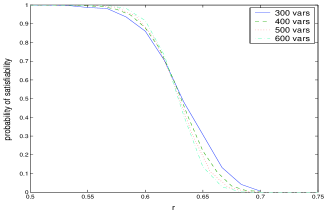
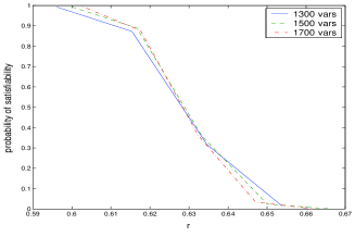
Figure 1: The probability of satisfiability as a function of $r$ for $n=300,400,500$ and $600$.

4 Conclusion

We have placed a lower bound of $r^{*}>0.546$ on the threshold of the phase-transition in EC3. Combined with the upper bound of $r^{*}<0.644$ [5], a fairly small gap of $0.098$ remains. It might be possible to improve our lower bound using algorithms that choose a variable based on the number of its occurrences in the remaining formula, as in [16, 18].

5 Acknowledgements

The authors thank Sahar Abubucker and Arthur Chtcherba for reading the manuscript and providing valuable comments. This work was supported in part by NSF grants PHY-0200909, PHY-0071139 and the Sandia University Research Project.

References

- [1] Theoretical Computer Science 265 (2001), Special Issue on NP-Hardness and Phase Transitions.
- [2] A. M. Childs, E. Farhi and J. Preskill, Robustness of adiabatic quantum computation, Physical Review A, 65 (2002), 012322.
- [3] Wenjin Mao, Quantum algorithm to solve satisfiability problems, quant-ph/0411194.
- [4] D. Achlioptas, A. Chtcherba, G. Istrate and C. Moore, The phase transition in 1-in- SAT and NAE 3-SAT, SODA (2001) 721–722.
- [5] S. Knysh, V.N. Smelyanskiy and R.D. Morris, Approximating satisfiability transition by suppressing fluctuations, quant-ph/0403416.
- [6] N. Wormald, Differential equations for random processes and random graphs, Annals of Applied Probability 5 (4) (1995) 1217-1235.
- [7] E. Farhi, J. Goldstone, S. Gutmann, J. Lapan, A. Lundgren and D. Preda, A quantum adiabatic evolution algorithm applied to random instances of an NP-complete problem, Science 292 (2001) 472-474, quant-ph/0104129.
- [8] W. van Dam, M. Mosca and Umesh Vazirani, How powerful is adiabatic quantum computation? FOCS (2001) 279-287, quant-ph/0206003.
- [9] E. Farhi, J. Goldstone and S. Gutmann, A numerical study of the performance of a quantum adiabatic evolution algorithm for satisfiability, quant-ph/0007071.
- [10] S. Malik, M. W. Moskewicz, C. F. Madigan, Y. Zhao and L. Zhang, Chaff: Engineering an efficient SAT solver, DAC (2001), 530-536.
- [11] D. Achlioptas, A survey of lower bounds for random 3-SAT via differential equations, Theoretical Computer Science 265, Special Issue on NP-Hardness and Phase Transitions (2001) 159-185.
- [12] M.-T. Chao and J. Franco, Probabilistic analysis of a generalization of the unit-clause literal selection heuristics for the -satisfiability problem, Information Science 51 (3) (1995) 289-314.
- [13] D. Achlioptas and M. Molloy, The Analysis of a list coloring algorithm on a random graph.” FOCS (1997) 204-213.
- [14] A. Frieze and S. Suen, Analysis of two simple heuristics on a random instance of -SAT, J. Algorithms, 20 (2) (1996) 312-355.
- [15] E. Friedgut, Sharp thresholds of graph properties, and the k-SAT problem, J. Amer. Math. Soc. 12 (1999) 1017-1054.
- [16] D. Achlioptas and C. Moore, Almost all graphs with average degree 4 are 3 colorable, STOC (2002) 199-208.
- [17] Chu Min Li and Anbulagan, Heuristics based on unit-propagation for satisfiability problems, IJCAI (1997), 366-371.
- [18] A.C. Kaporis, L. M. Kirousis and E. M. Lalas, The probabilistic analysis of a greedy satisfiability algorithm, ESA (2002).