Lessons from Three Views of the Internet Topology

Abstract

Network topology plays a vital role in understanding the performance of network applications and protocols. Thus, recently there has been tremendous interest in generating realistic network topologies. Such work must begin with an understanding of existing network topologies, which today typically consists of a relatively small number of data sources. In this paper, we calculate an extensive set of important characteristics of Internet AS-level topologies extracted from the three data sources most frequently used by the research community: traceroutes, BGP, and WHOIS. We find that traceroute and BGP topologies are similar to one another but differ substantially from the WHOIS topology. We discuss the interplay between the properties of the data sources that result from specific data collection mechanisms and the resulting topology views. We find that, among metrics widely considered, the joint degree distribution appears to fundamentally characterize Internet AS-topologies: it narrowly defines values for other important metrics. We also introduce an evaluation criteria for the accuracy of topology generators and verify previous observations that generators solely reproducing degree distributions cannot capture the full spectrum of critical topological characteristics of any of the three topologies. Finally, we release to the community the input topology datasets, along with the scripts and output of our calculations. This supplement should enable researchers to validate their models against real data and to make more informed selection of topology data sources for their specific needs.

1 Introduction

Internet topology analysis and modeling has attracted substantial attention recently [1, 2, 3, 4, 5, 6, 7, 8]. Such an interest is not surprising since the Internet’s topological properties and their evolution are cornerstones of many practical and theoretical network research agendas. Our own motivation for this study is the need to construct accurate network emulation environments [11] that will enable development, reliable testing, and performance evaluation of new applications, protocols, and routing architectures [10]. Knowledge of realistic network topologies and the availability of tools to generate them are essential to this goal. We also seek to develop a methodology to compare topologies to one another based on relatively simple metrics. That is, we seek a set of metrics such that when two topologies demonstrate similar values for a particular property, they will be similar across a broad range of potential properties.

There are a number of sources of Internet topology data, obtained using different methodologies that yield substantially different topological views of the Internet. Unfortunately, many researchers either rely only on one data source, sometimes outdated or incomplete, or mix disparate data sources into one topology. To date, there has been little attempt to provide a detailed analytical comparison of the most important properties of topologies extracted from the different data sources.

Our study fills this gap by analyzing and explaining topological properties of Internet AS-level graphs extracted from the three commonly used data sources: (1) traceroute measurements [12]; (2) BGP [13]; and (3) the WHOIS database [14]. This work makes three key contributions to the field of topology research:

1. We calculate a broad range of topology metrics considered in the networking literature for the three sources of data. We reveal the peculiarities of each data source and the resulting interplay between artifacts of data collection and the key properties of the derived graphs.

2. We highlight the interdependencies between a broad array of topological features and discuss their relevance when comparing Internet topologies to various random graph models that attempt to capture Internet topology characteristics. Our analysis shows that graph models that reproduce the joint degree distribution of the graphs also capture other crucial topological characteristics to best approximate the topology.

3. To promote and simplify further analysis and discussion, we release [15] the following data and results to the community: a) the AS-graphs representing the topologies extracted from the raw data sources; b) the full set of data plots (many not included in the paper) calculated for all graphs; c) the data files associated with the plots, useful for researchers looking for other summary statistics or for direct comparisons with empirical data; and d) the scripts and programs we developed for our calculations.

We organize this paper as follows. Section 2 describes our data sources and how we constructed AS-level graphs from these data. In Section 3 we present the set of topological characteristics calculated from our graphs and explain what they measure and why they are important. Section 4 compares properties of the observed topologies with classes of random graphs and discusses the accuracy criteria for topology generators. We discuss the limitations of our study in Section 5. We conclude in Section 6 with the summary of our findings.

2 Construction of AS-level graphs

2.1 Data sources

We used the following data sources to construct AS-level graphs of the Internet: traceroute measurements, BGP data, and the WHOIS database.

Traceroute [16] is a tool that captures a sequence of IP hops along the forward path from the source to a given destination by sending either UDP or ICMP probe packets to the destination.

CAIDA has developed a tool, skitter [12], to collect continuous traceroute-based Internet topology measurements. AS-level topology graphs derived from the skitter data on a daily basis are available for download at [17]. For this study, we used the 31 daily graphs for the month of March 2004. The measurements contain multi-origin ASes (prefixes announced by different originating ASes) [18], AS-sets [19], and private ASes [20]. Both multi-origin ASes and AS-sets create ambiguous mapping between IP addresses and ASes, while private ASes create false links. Hence we filter AS-sets, multi-origin ASes, and private ASes from each graph, and we discard indirect links [17]. We then merge the each daily graph to form one graph referred to as the skitter graph throughout the rest of the paper.

BGP (Border Gateway Protocol) [19] is the protocol used for routing among ASes in the Internet. RouteViews [13] collects and archives both static snapshots of the BGP routing tables and dynamic BGP data in the form of BGP message dumps (updates and withdrawals). Therefore, we derive two types of graphs from the BGP data for the same month of March 2004: one from the static tables (BGP tables) and one from the updates (BGP updates). In both cases, we filter AS-sets and private ASes and merge the 31 daily graphs into one.

WHOIS [14] is a collection of databases containing a wide range of information useful to network operators. Unfortunately, these databases are manually maintained with little requirements for updating the registered information in a timely fashion. RIPE’s [21, 22] WHOIS database contains the most reliable current topological information, although it covers primarily European Internet infrastructure.

We obtained the RIPE WHOIS database dump for April 07, 2004. The records of interest to us are:

aut-num:	ASx
import:	from ASy
export:	to ASz

which indicate links ASx-ASy and ASx-ASz. We construct an AS-level graph (referred to as WHOIS graph) from these data and exclude ASes that did not appear in the aut-num lines. Such ASes are external to the database and we cannot correctly estimate their topological properties (e.g. node degree). We also filter private ASes.

All four graphs constructed as described are available for download from [15]. Overlap statistics of the graphs are shown in Table 1.

Table 1: Comparison of graphs built from different data sources. The baseline graph $G_{A}$ is the BGP-tables graph. Graph $G_{B}$ is one the other graphs listed in the first row.

	BGP updates	skitter	WHOIS
Number of nodes in both $G_{A}$ and $G_{B}$ ($|V_{A}\bigcap V_{B}|$)	17,349	9,203	5,583
Number of nodes in $G_{A}$ but not in $G_{B}$ ($|V_{A}\setminus V_{B}|$)	97	8,243	11,863
Number of nodes in $G_{B}$ but not in $G_{A}$ ($|V_{B}\setminus V_{A}|$)	68	1	1,902
Number of edges in both $G_{A}$ and $G_{B}$ ($|E_{A}\bigcap E_{B}|$)	38,543	17,407	12,335
Number of edges in $G_{A}$ but not in $G_{B}$ ($|E_{A}\setminus E_{B}|$)	2,262	23,398	28,470
Number of edges in $G_{B}$ but not in $G_{A}$ ($|E_{B}\setminus E_{A}|$)	3,941	11,552	44,614

Comparing the two BGP-derived graphs, we note that the sets of their constituent nodes and links are similar. Given minor differences between node and link sets of the BGP table- and update-derived topologies, we, not surprisingly, found the metric values calculated for these two graphs to be close. Therefore, in the rest of this study we present characteristics of the static BGP-table graph only and refer to it as BGP graph.

In constructing the skitter graph, we used BGP tables to map IP addresses observed in traceroutes to AS numbers. Therefore the number of nodes seen by skitter but not by BGP should be $0$. The one node difference (AS2277 Ecuanet in skitter data) results from the fact that different BGP table dumps were used to construct the BGP-table graph and to map an IP address to this AS on the day when skitter observed this IP address in its traces.

Based on the very method of their construction, the three graphs in this study reveal different sides of the actual Internet AS-level topology. The skitter graph closely reflects the topology of actual Internet traffic flows, i.e. the data plane. The BGP graph reveals the topology seen by the routing system, i.e. the control plane. However, both skitter and BGP are traceroute-like explorations of the network topology, meaning that we can try to approximate these graphs by a union of spanning trees rooted at, respectively, skitter monitors or BGP data collection points. As such, both these methods discover more radial links, that is, links connecting numerous low-degree nodes (e.g. customers ASes) to high-degree nodes (e.g. large ISP ASes). At the same time, these measurements fail to detect many tangential links, that is, links between nodes of similar degrees. Traceroute-like methods are particularly unsuitable for discovering tangential links interconnecting medium-to-low degree nodes (e.g. lower-tier ASes) since many of these links do not lie on any shortest path rooted at a particular vantage point in the core. In contrast, WHOIS data contains abundant medium-degree tangential links as directly attached to sources of WHOIS records (values of aut-num fields).

2.2 Statistical validity of our results

Lakhina et al. [24] numerically explored sampling biases arising from traceroute measurements and found that such traceroute-sampled graphs of the Internet yield insufficient evidence for characterizing the actual underlying Internet topology. However, Dall’Asta et al. [25] convincingly refute their conclusions by showing that various traceroute exploration strategies provide sampled distributions with enough signatures to distinguish at the statistical level between different topologies. The authors of [25] also argue that real mapping experiments observe genuine features of the Internet, rather than artifacts. These results lend credibility to our chosen traceroute-like data sources and imply that the real Internet topology is unlikely to be critically different from the ones measured in skitter and BGP cases.

The topology metrics we consider in Section 3 all show that the WHOIS topology is different from the other two graphs. Thus, the following question arises: Can we explain the difference by the fact that the WHOIS graph contains only a part of the Internet, namely European ASes? To answer this question we performed the following experiment. We considered the BGP-tables and WHOIS topologies narrowed to the set of nodes present both in BGP tables and WHOIS (cf. Table 1) and compared the various topological characteristics for the full and the reduced graphs. Results of this comparison are available in the Supplement [15]. We found that the induced graphs preserve the full set of the properly normalized topological properties of the original graphs. Therefore, the differences between full BGP and WHOIS topologies are intrinsic to their originating data sources, and not due to geographical biases in sampling the Internet.

3 Topology characteristics

In this section, we quantitatively analyze differences between the three graphs in terms of various topology metrics. The set of metrics we discuss here encompasses most of the graph metrics considered relevant for topology in the networking literature [3, 4, 5, 8]. Relative to most related work, we consider a broader array of metrics of interest.

For each metric, we address the following points: 1) metric definition; 2) metric importance; and 3) discussion on the metric values for the three measured topologies. We present these results in the plots associated with every metric and in the master Table 3 containing all the scalar metric values for all the three graphs.

We start with simple and basic metrics that characterize local connectivity in a network. With increasing precision, we move on to more sophisticated metrics that describe global properties of the topology. The latter metrics play a vital role in the performance of network protocols and applications. Some metrics that we discuss here are not exactly equal but directly related to a topology characteristic deemed important in the networking literature. Where possible, we illuminate the relationship between the metrics we consider and the ones that have been discussed in influential networking papers. We provide a summary of this mapping in Table 2.

Table 2: Important metric mappings.

Previously defined metric	Our definition
Likelihood in [4]	Assortativity coefficient
Expansion in [3]	Distance
Resilience in [3]
Performance in [4]	Spectrum
Link value in [3]
Router utilization in [4]	Betweenness

3.1 Average degree

Definition. The two most basic graph properties are the number of nodes $n$ (also referred as graph size) and the number of links $m$. They define the average node degree $\bar{k}=2m/n$.

Importance. Average degree is the coarsest connectivity characteristic of the topology. Networks with higher $\bar{k}$ are “better-connected” on average and, consequently, are likely to be more robust. Detailed topology characterization based only on the average degree is rather limited, since graphs with the same average node degree can have vastly different structures.

Discussion. BGP sees almost twice as many nodes as skitter (Table 3). The WHOIS graph is smallest, but its average degree is almost three times larger than that of BGP, and $\sim 2.5$ times larger than that of skitter. In other words, WHOIS contains substantially more links, both in the absolute ($m$) and relative ($\bar{k}$) senses, than any other data source, but credibility of these links is lowest (cf. Section 2.1): there have been reports about some ISPs that tend to enter inaccurate information in the WHOIS database in order increase their “importance” in the Internet hierarchy [21].

Graphs ordered by increasing average degree $\bar{k}$ are BGP, skitter, WHOIS. We call this order the $\mathbf{\bar{k}}$-order.

3.2 Degree distribution

Definition. Let $n(k)$ be the number of nodes of degree $k$ ($k$-degree nodes). The node degree distribution is the probability that a randomly selected node is $k$-degree: $P(k)=n(k)/n$. The degree distribution contains more information about connectivity in a given graph than the average degree, since given a specific form of $P(k)$ we can always restore the average degree by $\bar{k}=\sum_{k=1}^{k_{max}}kP(k)$, where $k_{max}$ is the maximum node degree in the graph. If the degree distribution in a graph of size $n$ is a power law, $P(k)\sim k^{-\gamma}$, where $\gamma$ is a positive exponent, then $P(k)$ has a natural cut-off at the power-law maximum degree [9]: $k_{max}^{PL}=n^{1/(\gamma-1)}$.

Importance. The degree distribution is the most frequently used topology characteristic. The observation [1] that the Internet’s degree distribution follows power law had significant impact on network topology research: Internet models before [1] failed to exhibit power laws. Since power law is a highly variable distribution, node degree is an important attribute of an individual node. For example, we can use AS degrees as the simplest way to rank ASes [26].

Discussion. As expected, the degree distribution PDFs and CCDFs in Figure 1 are in the $\bar{k}$-order (BGP $<$ skitter $<$ WHOIS) for a wide range of node degrees.

Comparing the observed maximum node degrees $k_{max}$ with those predicted by the power law $k_{max}^{PL}$ in Table 3, we conclude that skitter is closest to power law. The power-law approximation for the BGP graph is less accurate. The WHOIS graph has an excess of medium degree nodes and its node degree distribution does not follow power law at all. It is not surprising then that augmenting the BGP graph with WHOIS links breaks the power law characteristics of the BGP graph [2, 22].

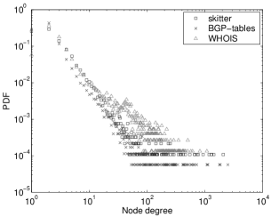
(a) PDF

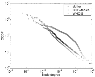
(b) CCDF

(c) PDFs of skitter vs. BGP differences

Figure 1: Node degree distributions $\mathbf{P(k)}$.

Note that there are fewer 1-degree nodes than 2-degree nodes in all the graphs (cf. Figure 1(a)). This effect is due to the AS number assignment policies [20] allowing a customer to have an AS number only if it has multiple providers. If these policies were strictly enforced, then the minimum AS degree would be 2.

CCDFs of skitter and BGP graphs look rather similar (Figure 1(b)), but Table 1 shows significant differences between the two graphs, in terms of (non-)intersecting nodes and links. We seek to answer the question of where, topologically, these nodes and links are located. Calculating the degree distribution of nodes present only in the BGP graph (Figure 1(c)), we detect a skew towards low-degree nodes. The average degree of the nodes that are present only in BGP graphs, and not in skitter is $1.86$. Skitter’s target list of destinations to probe does not contain any replying IP address in the address blocks advertised by these small ASes. As a result, the skitter graph misses them.

Most links present only in BGP, but not in skitter, are tangential links between low-degree ASes (see [15] for details). The majority of such links connect the low-degree ASes present only in BGP to their secondary (backup) low-degree providers, while their primary providers are of high degrees. Even if skitter detects a low-degree AS having such a small backup provider, this tool is still unlikely to detect the backup link since its traceroutes follow the primary path via the large provider.

3.3 Joint degree distribution

While the node degree distribution tells us how many nodes of given degree are in the network, it fails to provide information on the interconnection between these nodes: given $P(k)$, we still do not know anything about the structure of the neighborhood of the average node of a given degree. The joint degree distribution (or degree-degree correlation matrix) fills this gap by providing information about nodes’ 1-hop neighborhoods.

Definition. Let $m(k_{1},k_{2})$ be the total number of edges connecting nodes of degrees $k_{1}$ and $k_{2}$. The joint degree distribution (JDD) is the probability that a randomly selected edge connects $k_{1}$- and $k_{2}$-degree nodes: $P(k_{1},k_{2})\sim m(k_{1},k_{2})/m$. Note that $P(k_{1},k_{2})$ is different from the conditional probability $P(k_{2}|k_{1})=\bar{k}/k_{1}P(k_{1},k_{2})/P(k_{1})$ that a given $k_{1}$-degree node is connected to a $k_{2}$-degree node. The JDD contains more information about the connectivity in a graph than the degree distribution, since given a specific form of $P(k_{1},k_{2})$ we can always restore both the degree distribution $P(k)$ and average degree $\bar{k}$ by expressions in [9]. The JDD is a function of two arguments. A summary statistic of JDD, that is a function of one argument is called the average neighbor connectivity $k_{nn}(k)=\sum_{k^{\prime}=1}^{k_{max}}k^{\prime}P(k^{\prime}|k)$. It is simply the average neighbor degree of the average $k$-degree node. It shows whether ASes of a given degree preferentially connect to high- or low-degree ASes. In a full mesh graph, $k_{nn}(k)$ reaches its maximal possible value $n-1$. Therefore, for uniform graph comparison we plot normalized values $k_{nn}(k)/(n-1)$. We can further summarize JDD by a single scalar called assortativity coefficient $r$ [27, 28].

Importance. As opposed to the degree distribution, the network community has recently started recognizing the importance on JDD [29, 6]. The most prominent recent example defines likelihood [4]—the central metric for their argument—as a metric directly related to the assortativity coefficient. They propose to use likelihood as a measure of randomness differentiating between multiple graphs with the same degree distribution. Such a measure is important for evaluating the amount of order (e.g. engineering design constraints) present in a given topology. A topology with low likelihood is not random, it is a result of some sophisticated evolution processes involving specific design purposes. We actively use the JDD in the described fashion in Section 4.

The assortativity coefficient $r$ ( $-1\leqslant r\leqslant 1$) has direct practical implications. Disassortative networks with $r<0$ have an excess radial links connecting nodes of dissimilar degrees. Such networks are vulnerable to both random failures and targeted attacks. Viruses spread faster in these topologies. On a positive side, vertex cover in disassortative graphs is smaller, which is important for applications such as traffic monitoring [30] and prevention of DoS attack [31]. The opposite properties apply to assortative networks with $r>0$ that have an excess of tangential links connecting nodes of similar degrees.

Discussion. All the three Internet graphs built from our data sources are disassortative ($r<0$) as seen in Table 3. We call the order of graphs with decreasing assortativity coefficient $r$—WHOIS, BGP, skitter—the $\mathbf{r}$-order. The most disassortative graph is skitter, that has the largest excess of radial links. The least disassortative graph is WHOIS. The $r$-order can be explained in terms of differing topology measurement methodologies. As described in Section 2, the traceroute-like explorations of BGP and skitter data fail to detect tangential links, thus causing the graphs to be disassortative. The WHOIS graph’s collection methodology however finds abundant medium-degree tangential links, resulting in the graph’s higher assortative value.

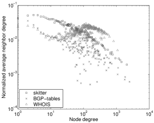
Figure 2: Normalized average neighbor connectivity $\mathbf{k_{nn}(k)/(n-1)}$.

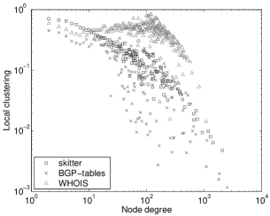
Figure 3: Local clustering $\mathbf{C(k)}$.

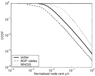
Figure 4: Rich club connectivity $\mathbf{\phi(\rho/n)}$.

The interplay between $\bar{k}$- and $r$-orders underlies Figure 4, where we show the average neighbor connectivity functions for the three graphs. Skitter has the largest excess of radial links that connect low-degree nodes (customers ASes) to high-degree nodes (large provider ASes). The high radial links are responsible for skitter’s highest average degree for the neighbors of low-degree nodes: in Figure 4, skitter is at the top in the area of low degrees, which follows the $r$-order. On the other hand, the greatest proportion of tangential links between ASes of similar degrees in WHOIS graph contributes to connectivity of neighbors of high-degree nodes; therefore the WHOIS graph is at the top for high degree nodes ($\bar{k}$-order).

Note that in the case of skitter and BGP, $k_{nn}(k)$ can be approximated by a power law with the corresponding exponents $\gamma_{nn}$ in Table 3.

3.4 Clustering

While the JDD contains information about the degrees of neighbors for the average $k$-degree node, it does not tell us how these neighbors interconnect. Clustering satisfies this need by providing a measure of how close a node’s neighbors are to forming a clique.

Definition. Let $\bar{m}_{nn}(k)$ be the average number of links between the neighbors of $k$-degree nodes. Local clustering is the ratio of this number to the maximum possible such links: $C(k)=2\bar{m}_{nn}(k)/k/(k-1)$. If two neighbors of a node are connected, then these three nodes together form a triangle (3-cycle). Therefore, by definition, local clustering is the average number of 3-cycles involving $k$-degree nodes. The two summary statistics associated with local clustering are mean local clustering $\bar{C}=\sum C(k)P(k)$, which is the average value of $C(k)$, and the clustering coefficient $C$, which is the percentage of 3-cycles among all connected node triplets in the entire graph (for exact definition, see [32]).

Importance. Similar to the JDD, one can use clustering as a litmus test for verifying the accuracy of a topology model or generator [5]. Clustering is a basic connectivity characteristic. Therefore, if a model reproduces clustering incorrectly, it is likely to be less accurate for a variety of graph characteristics. We use clustering to verify the efficacy of topology models in Section 4.

Clustering is practical because it expresses local robustness in the graph: the higher the local clustering of a node, the more interconnected are its neighbors, thus increasing the path diversity locally around the node. Virus outbreaks spread faster in high-clustered networks, although outbreak sizes are smaller [33]. Networks with strong clustering are likely to be chordal or of low chordality, which makes certain routing strategies perform better [34].

Discussion. We first observe that the clustering average values $\bar{C}$ in Table 3 are in the $\bar{k}$-order, which is expected: more the links, more the clustering. The values of $\bar{C}$ are almost equal for skitter and WHOIS, but the clustering coefficient $C$ is 15 times larger for WHOIS than for skitter. As shown in [35], orders of magnitude difference between $\bar{C}$ and $C$ is intrinsic to highly disassortative networks and is a consequence of degree correlations (JDD).

Similarly to $k_{nn}(k)$, the interplay between $\bar{k}$- and $r$-orders explains Figure 4, where we plot local clustering as a function of node degree $C(k)$. For low degree nodes, skitter’s clustering is the highest amongst the three graphs because skitter graph is most disassortative. The links adjacent to low-degree nodes are most likely to lead to high-degree nodes, the latter being interconnected with a high probability. For high degree nodes, the WHOIS graph exhibits highest values for clustering since this graph has the highest average connectivity (largest $\bar{k}$). The neighbors of high-degree nodes are interconnected to a greater extent resulting in higher clustering for such nodes.

Similar to $k_{nn}(k)$, $C(k)$ also can be approximated by a power law for skitter and BGP graphs (exponents $\gamma_{C}$ in Table 3).

JDDs with strong correlations play a major part for the presence of non-trivial clustering observed in many networks [35]. This interplay explains overall similarity between degree correlations and clustering, in general, and similarity between $k_{nn}(k)$ and $C(k)$, in particular.

3.5 Rich club connectivity

Definition. Let $\rho=1\ldots n$ be the first $\rho$ nodes ordered by their non-increasing degrees in a graph of size $n$. Rich club connectivity (RCC) $\phi(\rho/n)$ is the ratio of the number of links in the subgraph induced by the $\rho$ largest-degree nodes to the maximum possible links $\rho(\rho-1)/2$. In other words, the RCC is a measure of how close $\rho$-induced subgraphs are to cliques.

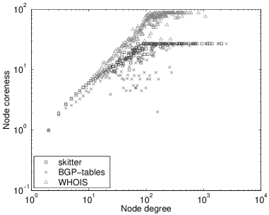
Figure 5: Average coreness of $k$-degree nodes $\mathbf{\kappa(k)}$.

Importance. As of this writing, one of the more successful Internet AS-level topology model is the Positive Feedback Preference (PFP) model by Zhou and Mondragon [8]. It accurately reproduces a wide spectrum of metrics of the measured AS-level topology by trying to explicitly capture only the following three characteristics: (i) the exact form of the node degree distribution; (ii) the maximum node degree; and (iii) RCC. The success of the PFP model in approximating the real topology is yet to be fully explained. One can show that networks with the same JDDs have the same RCC. The converse is not true, but one can fully describe all the JDDs having a given form of RCC.

Discussion. As expected, the values of $\phi(\rho/n)$ in Figure 4 are in the $\bar{k}$-order with WHOIS at the top: more links result in denser cliques. RCC exhibits clean power laws for all three graphs in the area of medium and large $\rho/n$. The values of the power-law exponents $\gamma_{rc}$ in Table 3 result from fitting $\phi(\rho/n)$ with power laws for 90% of the nodes, $0.1\leqslant\rho/n\leqslant 1$.

3.6 Coreness

Definition. There are two definitions of coreness. In graph-theoretic literature [36], the $k$-core of a graph is the subgraph obtained from the original graph after removal of all nodes of degree less than or equal to $k$. A more informative definition of $k$-core [7] is the subgraph obtained from the original graph by the iterative removal of all nodes of degree less than or equal to $k$. We use the latter definition. The node coreness $\kappa$ of a given node is then the maximum $k$ such that this node is still present in the $k$-core but removed in the $(k+1)$-core. The minimum node coreness in a given graph is $\kappa_{min}=k_{min}-1$, where $k_{min}$ is the lowest node degree present. All 1-degree nodes have $\kappa=0$. The maximum node coreness $\kappa_{max}$ in a graph, or the graph coreness, is such that the $\kappa_{max}$-core is not empty, but $(\kappa_{max}+1)$-core is. For example, coreness of a tree is $0$ and coreness of a $k$-regular graph [37] is equal to coreness of all of its nodes (all having degree $k$), which is $k-1$. We further define the graph core as its $\kappa_{max}$-core, and the graph fringe as the set of nodes with minimum coreness $\kappa_{min}$. Note that because the process of building core is iterative, nodes with degree $k>\kappa_{min}$ can be in the fringe.

Importance. The node coreness tells us how “deep in the core” the node is. It is a much more sophisticated measure of node connectivity than node degree. Indeed, the node degree can be high, but if its coreness is small, then the node is not well connected and one can easily disconnect it by removing its poorly connected neighbors. For example, a high-degree hub of a star has coreness of $0$. At the same time, node coreness is not a measure of centrality of the node. For example, a low-degree node interconnecting a few high-degree hubs has a low value of coreness, but intuitively it is in the “center of the graph.” At the same time, coreness is important for topology visualization capable of revealing network architectural fingerprints [38] and signatures of topology dynamics under different types of anomalies (worm and DoS attacks, outages, misconfigurations, etc.) [7].

Discussion. The average node coreness in Table 3 is in the $\bar{k}$-order, which is expected. The graph coreness of WHOIS is more that three times larger than of skitter and BGP. WHOIS has particularly large core size and graph coreness because the $r$-order amplifies the $\bar{k}$-order in this case: WHOIS has highest link density (largest $\bar{k}$) and highest concentration of them in the core (largest $r$). WHOIS graph has the largest relative core size and smallest relative fringe size (cf. Table 3). The BGP graph is the sparsest, having the smallest relative core size and the largest relative fringe size. Interestingly, in the BGP graph, nodes with degree as low as 34 are in the core, and nodes with degree as high as 7 are in the fringe. For all three graphs, the average node coreness as a function of node degree $\kappa(k)$ roughly follows power laws for $k\lesssim 100$ (Figure 5). The corresponding exponents and mean coreness are given in Table 3. For nodes with degrees $k\gtrsim 100$ the coreness reaches saturation: increasing node degree above $100$ does not increase coreness.

3.7 Distance

Definition. The shortest path length distribution or simply the distance distribution $d(x)$ is the probability for a random pair of nodes to be at a distance $x$ hops from each other. Two basic summary statistics associated with the distance distribution of a graph are average distance $\bar{d}$ and the standard deviation $\sigma$. We call the latter the distance distribution width since distance distribution in Internet graphs (and in many other networks) has a characteristic Gaussian-like shape.

Eccentricity is an extreme form of distance: if $d_{ij}$ is distance between nodes $i$ and $j$, then eccentricity $\varepsilon_{i}$ of node $i$ is the maximum distance from $i$ [37]: $\varepsilon_{i}=\max_{j}d_{ij}$. The maximum eccentricity in a graph is also the maximum distance and is called the graph diameter $D=\varepsilon_{max}$, and the minimum eccentricity $R=\varepsilon_{min}$ is called the graph radius. The set of nodes with maximum eccentricity forms graph periphery, while nodes with minimum eccentricity belong to graph center [37].

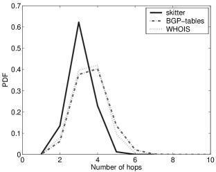
Figure 6: Distance $\mathbf{d(x)}$ distribution.

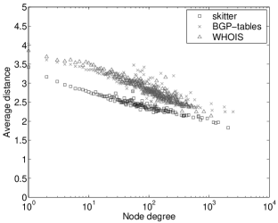
Figure 7: Average distance from $k$-degree nodes $\mathbf{d(k)}$.

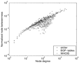
Figure 8: Normalized node betweenness $\mathbf{B(k)/n/(n-1)}$.

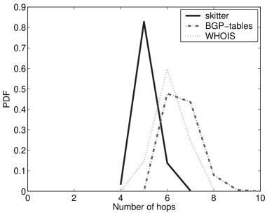
Figure 9: Eccentricity $\mathbf{\varepsilon(k)}$ distribution.

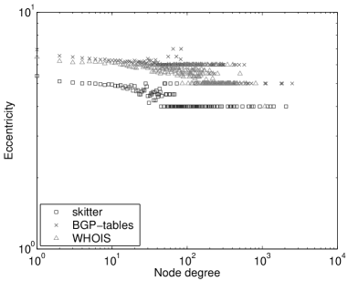
Figure 10: Average eccentricity from $k$-degree nodes $\mathbf{\varepsilon(k)}$.

Importance. Distance distribution is critically important for many applications, the most prominent being routing. Distance-based locality-sensitive approach [39] is the root of most modern routing algorithms. As shown in [40], performance parameters of these algorithms depend strongly on the distance distribution in a network. In particular, short average distance and narrow distance distribution width break the efficiency of traditional hierarchical routing. They are among the root causes of interdomain routing scalability issues in the Internet today.

Distance distribution also plays a vital role in robustness of the network to viruses. Viruses can quickly contaminate larger portions of a network that has small distances between nodes. Topology models that accurately reproduce observed distance distribution will benefit researchers, who are developing techniques to quarantine the network from viruses. Finally, expansion from the seminal paper [3], identified as a critical metric for topology comparison analysis, is a renormalized version of distance distribution.

Discussion. Interestingly enough, although the distance distribution is a “global” topology characteristic, we can explain Figure 8 by the interplay between our local connectivity characteristics: the $\bar{k}$- and $r$-orders. First, we note that the skitter graph stands out in Figure 8 as it has the smallest average distance and the smallest distribution width (cf. Table 3). This result appears unexpected at first since the skitter graph has more nodes than the WHOIS graph and only about half the number of links. One would expect a denser graph (WHOIS) to have a lower average distance since adding links to a graph can only decrease the average distance in it. Surprisingly, the average distance of the most richly connected (highest $\bar{k}$) WHOIS graph is not the lowest. This result can be explained using the $r$-order. Indeed, a more disassortative graph has a greater proportion of radial links, shortening the distance from the fringe to the core. The skitter graph has the right balance between the relative number of links $\bar{k}$ and their radiality $r$, that minimizes the average distance. Compared to skitter, the BGP graph has larger distance because it is sparser (lower $\bar{k}$), and the WHOIS graph has larger distance because it is more assortative (higher $r$).

The fact that 62% of AS paths in the skitter graph are 3-hop paths suggests the most frequent path pattern reflecting the customer-provider AS hierarchy: source’s AS in the fringe $\rightarrow$ source’s provider AS in the core $\rightarrow$ destination’s provider AS in the core $\rightarrow$ destination’s AS in the fringe.

Another important observation is that for all three graphs, including WHOIS, the average distance as a function of node degree exhibits relatively stable power laws in the full range of node degrees (Figure 8), with exponents given in Table 3.

Both the eccentricity distribution $\varepsilon(x)$ (Figure 9) and average eccentricity from $k$-degree nodes $\varepsilon(k)$ (Figure 10) are similar to their averaged distance counterparts. Table 3 also shows diameter, radius and average eccentricity for our graphs, as well as the relative size of graph center and periphery. In the WHOIS graph, the center consists of only one AS, AS702 (UUNET), uniquely positioned to have the minimum eccentricity of $4$. If we add the nodes having eccentricity of $5$, the center would consist of 1109 ASs, the center size ratio $n_{R}/n=0.15$ would become the largest among all three graphs, and it would be in the expected $\bar{k}$-order.

3.8 Betweenness

Average distance is a good node centrality measure: intuitively, nodes with smaller average distances are closer to the graph “center.” However, the most commonly used measure of centrality is betweenness. It is applicable not only to nodes, but also to links.

Definition. Let $\sigma_{ij}$ be the number of shortest paths between nodes $i$ and $j$ and $l$ be either a node or link. Let $\sigma_{ij}(l)$ be the number of shortest paths between $i$ and $j$ going through node (or link) $l$. Its betweenness is $B_{l}=\sum_{ij}\sigma_{ij}(l)/\sigma_{ij}$. The maximum possible value for node and link betweenness is $n(n-1)$ [25], therefore in order to compare betweenness in graphs of different sizes, we normalize it by $n(n-1)$.

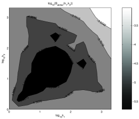
(a) skitter

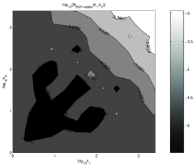
(b) BGP tables

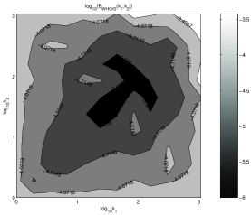
(c) WHOIS

Figure 11: Logarithm of normalized link betweenness $\mathbf{B(k_{1},k_{2})/n/(n-1)}$ on a log-log scale.

Importance. Betweenness measures the number of shortest paths passing through a node or link and, thus, estimates the potential traffic load on this node/link assuming uniformly distributed traffic following shortest paths. Betweenness is important for traffic engineering applications that try to estimate potential traffic load on nodes/links and potential congestion points in a given topology. Betweenness is also critical for evaluating the accuracy of topology sampling by traceroute-like probes (e.g. skitter and BGP). As shown in [25], the broader the betweenness distribution, the higher the statistical accuracy of the sampled graph. The exploration process statistically focuses on nodes/links with high betweenness thus providing an accurate sampling of the distribution tail and capturing relevant statistical information. Finally we note that link value, used in [3] to analyze the topology hierarchy, and router utilization, used [4] to measure network performance, are both directly related to betweenness.

Discussion. The simplest approach to calculating node betweenness results in long running times, but we used an efficient algorithm from [41]. We also modified it to also compute link betweenness. For skitter and BGP graphs, node betweenness is a growing power-law function of node degree (Figure 8) with exponents given in Table 3. The WHOIS graph has an excess of medium degree nodes (cf. Figure 1) leading to greater path diversity and, hence, to lower betweenness values for these nodes. We also calculate average link betweenness as a function of degrees of nodes adjacent to a link $B(k_{1},k_{2})$ (Figure 11). Contrary to popular belief, the contour plots show that link betweenness does not measure link centrality. First, betweenness of links adjacent to low-degree nodes (the left and bottom sides of the plots) is not the minimum. In fact, non-normalized betweenness of links adjacent to 1-degree nodes is constant and equal to $n-1$ (the number of destinations in the rest of the network). Similar values of betweenness characterize links elsewhere in the graph, including radial links between high and low-to-medium degree nodes and tangential links in the zone of medium-to-high degrees (diagonal zone from bottom-right to upper-left). Second, while the maximum-betweenness links are between high-degree nodes as expected (the upper right corner of the plots), the minimum-betweenness links are tangential in the medium-to-low degree zone (diagonal areas of low values from bottom-left to upper-right). We can explain the latter observation by the following argument. Let $i$ and $j$ be two nodes connected by a minimum-betweenness link $l$. The only shortest paths going through $l$ are those between nodes that are below $i$ and $j$, where “below” means further from the core and closer to the fringe. When the degrees of both $i$ and $j$ are small, the numbers of nodes below them (with lower degree) are small, too. Consequently, the number of shortest paths, proportional to the product of the number of nodes below $i$ and $j$, attains its minimum at $l$. We conclude that link betweenness is not a measure of centrality but a measure of some combination of link centrality and radiality.

3.9 Spectrum

Definition. Let $\hat{a}$ be the adjacency matrix of a graph. This $n\times n$ matrix is constructed by setting the value of its element $a_{ij}=a_{ji}=1$ if there is a link between nodes $i$ and $j$. All other elements have value  $0$. Scalar $\lambda$ and vector $v$ are the eigenvalue and eigenvector respectively of $\hat{a}$ if $\hat{a}v=\lambda v$. The spectrum of a graph is the set of eigenvalues of its adjacency matrix.

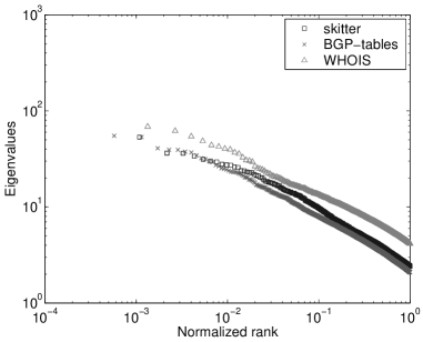
Figure 12: Spectrum. Absolute values of top 10% of eigenvalues ordered by their normalized rank: the absolute value divided by the total number of eigenvalues calculated for a given graph.

Importance. We stress that spectrum is one of the most important global characteristics of the topology. Spectrum yields tight bounds for a wide range of critical graph characteristics [42], such as distance-related parameters, expansion properties, and values related to separator problems estimating graph resilience under node/link removal. The largest eigenvalues are particularly important. Most networks with high largest eigenvalues have small diameter, expand faster, and are more robust. To further emphasize the importance of spectrum, we consider the following two specific examples of spectrum-related metrics that played a central role in two significant contributions to networking topology research.

First, Tangmunarunkit et al. [3] defined network resilience, one of the three metrics critical for their topology comparison analysis, as a measure of network robustness under link removal, which equals the minimum balanced cut size of a graph. By this definition, resilience is related to spectrum since the graph’s largest eigenvalues provide bounds on network robustness with respect to both link and node removals [42].

Second, Li et al. [4] define network performance, one of the two metrics critical for their HOT argument, as the maximum traffic throughput of the network. By this definition, performance is related to spectrum since it is essentially the network conductance [43]. It can be tightly estimated by the gap between the first and second largest eigenvalues [42].

Beyond its significance for network robustness and performance, the graph’s largest eigenvalues are important for traffic engineering purposes since graphs with larger eigenvalues have, in general, more node- and link-disjoint paths to choose from. The spectral analysis of graphs is also a powerful tool for detailed investigation of network structure  [44, 45] , such as discovering clusters of highly interconnected nodes, and can reveal the hierarchy of ASes in the Internet [45].

Discussion. Our $\bar{k}$-order (BGP, skitter, WHOIS) plays a key role once again: the densest graph, WHOIS is on the top in Figure 12 and its first eigenvalue is largest in Table 3. The eigenvalue distributions of all the three graphs follow power laws.

Other important metrics such as coreness and eccentricity are explained in detail in the Supplement [15]. As with other metrics, the resulting metric values and differences in the three data sources can be explained using $\bar{k}$-order and $r$-order.

4 Observed topologies vs. random graph models

So far we have looked at metrics that provide important details about the Internet AS-graph. These metrics directly impact network applications and protocols, and can also be used to distinguish between different topologies. Using JDD, which determines both $\bar{k}$-order and $r$-order, we have been able to account for the differences and peculiarities in our target data sets. We next consider models that aim to reproduce observed topologies. In this section, we consider different classes of random graphs and discuss the relationship between these theoretical models and the Internet graphs we constructed from measurements. This analysis will help determine how close random graph models come to capturing measured Internet topologies.

4.1 Random graph models

Topology generators and models have been evolving steadily in the past few years. The simplest model mimicked the average degree observed in the topology. Given the number of nodes $n$ and edges $m$ (e.g. in the original graph), and, consequently, the average degree $\bar{k}=2m/n$, one can construct the class of maximally random graphs having the same average degree $\bar{k}$ by connecting every pair of nodes with probability $p=\bar{k}/n$. These graphs belong to the class of classical (Erdős-Rényi) random graphs $G_{n,p}$ [46]. In this paper we call such graphs 0K-random conceptualizing them as a zero-order approximation to the connectivity in the original graph. (We explain the exact semantics behind this terminology at the end of this section.) In general, 0K-random graphs fail to approximate real Internet topologies. In particular, the node degree distribution in 0K-random graphs is binomial, which is closely approximated by Poisson distribution $P_{0K}(k)=e^{-\bar{k}}\bar{k}^{k}/k!$ [9]. It is different from power-law degree distributions observed in the Internet.

The next model remedied this deficiency by capturing the degree distribution of the nodes. Given a specific form of the degree distribution $P(k)$ (e.g. extracted from the original graph), one can construct the class of maximally random graphs having the same degree distribution following, for example, a recipe introduced in [47, 48] and further formalized in [49]. We call such graphs 1K-random, and we can think of them as providing the first-order approximation to the connectivity of the original graph. Of particular interest for Internet modeling is the case when $P(k)$ is a power-law function [1]. The resulting sub-class of 1K-random graphs is called power-law random graphs (PLRG). Note that the 1K-random graphs have a specific form of the JDD $P(k_{1},k_{2})$ [9]. If we denote by $\tilde{P}(k)$ the probability that one of the two nodes adjacent to a randomly selected edge is of degree $k$, $\tilde{P}(k)=(k/\bar{k})P(k)$, then the JDD in 1K-random graphs is $P_{1K}(k_{1},k_{2})=\tilde{P}(k_{1})\tilde{P}(k_{2})$, meaning that there is no correlation between degrees of adjacent nodes. This is why 1K-random graphs are also called uncorrelated graphs. By construction [46], 0K-random graphs are also uncorrelated, with their JDD  $P_{0K}(k_{1},k_{2})$ given by the same expression as above, where $P(k)$ is the Poisson distribution $P_{0K}(k)$.

We now define a model that provides the next level of approximation: 2K-random graphs, which are maximally random graphs reproducing the given JDD $P(k_{1},k_{2})$. These graphs have the exact JDD as the original topology, but are random in all other respects. The semantics behind the “dK-random” notation becomes clear now: $d$ in “dK-random” is the number of arguments in the degree distribution function $P(k_{1},k_{2},\ldots,k_{d})$ that the dK-random graphs reproduce.

4.2 Comparison with observed topologies

As demonstrated in [3], 1K-random graphs produced by PLRG-based topology generators produce more accurate approximations of the Internet topology than outputs of older topology generators designed to simulate the perceived hierarchical structure of the Internet. We show that the topology generation strategy based on modeling only the degree distribution fails to attain the level of accuracy required in the description of Internet topology. Li et al.  [4] have shown that graphs with the same degree distribution can have different structures. In section 4.2.1, we compare the JDD of 1K-random graphs to the JDD observed in the measured data and show how they are different. As a next step, we also show how 2K-random graph models better approximate the real topologies.

4.2.1 Joint degree distribution

For each of our graphs, we consider its 1K-random counterpart reproducing $P(k)$ of the given graph. We calculate the JDD of the model and compare it with the actual JDDs of our graphs (Figure 13).

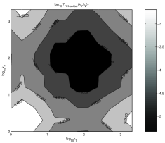
(a) 1K-random graph with skitter’s $P(k)$

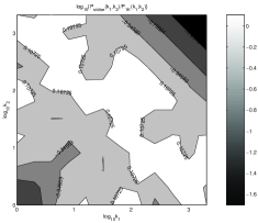
(b) skitter

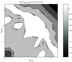
(c) BGP tables

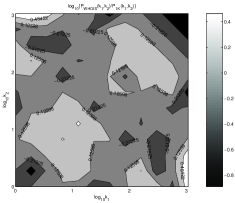
(d) WHOIS

Figure 13: Comparison of graphs with 1K-random models. a) The contour plot of the logarithm of the joint degree distribution $P_{1K}(k_{1},k_{2})$ for a 1K-random graph having the skitter degree distribution $P(k)$. b) The logarithm of the ratio of $P(k_{1},k_{2})$ observed in the real skitter graph to its simulated $P_{1K}(k_{1},k_{2})$. c, d) The plots, analogous to (b), for BGP and WHOIS graphs. Some asymmetry of the diagrams is due to interpolation and rounding algorithms in MATLAB. The scatter plots in the Supplement [15] are symmetric.

The 1K-random graph generated from skitter’s node degree distribution (Figure 13(a)) has the smallest frequency of tangential links interconnecting medium-degree nodes (the minimum in the center of the plot). The most frequent links are either radial (bottom-right and top-left corners) or low-degree tangential (bottom-left corner). The ratio of the actual JDD of the skitter graph to this model (Figure 13(b)) shows that the real skitter topology is quite different from its 1K-random version. The actual skitter graph exhibits a relative deficiency of links in the core and in the fringe (minimum of the ratio in the top-right and bottom-left corners). At the same time, it has a relative excess of radial links (bottom-right and top-left corners) and of tangential links in the medium-degree zone (the center of the plot).

The ratio of the BGP graph JDD to its 1K-random counterpart is similar to skitter ratio, but the excess of radial links is less prominent (Figure 13(c)). The ratio of the WHOIS graph JDD to its 1K-random model is less variable (Figure 13(d)) showing that the WHOIS graph is closer to being 1K-random than the other two graphs.

We now turn our attention to other JDD-derived statistics (cf. Section 3.3). The assortativity coefficient of uncorrelated 1K- and 0K-random graphs is $r=0$ and that their average neighbor connectivity $k_{nn}(k)$ is a constant function of node degree $k$ [9]. For 1K-random graphs, it is $k_{nn}^{1K}(k)=\langle k^{2}\rangle/\bar{k}$, where $\langle k^{2}\rangle$ denotes the second moment of the degree distribution. For 0K-random graphs, the expression is: $k_{nn}^{0K}(k)=\bar{k}+1$. While all three of our data sources yield disassortative graphs with $r<0$, the assortativity coefficient of the WHOIS graph is closest to $0$ (cf. Table 3). Its average neighbor degree $k_{nn}(k)$ varies within a factor of 2. In contrast, the average neighbor degree of the other two graphs varies by two orders of magnitude (cf. Figure 4). These observations again point out that the WHOIS graph is the closest to being 1K-random. Note, however, that PLRG-generated graphs [49, 3] cannot accurately approximate the WHOIS topology since its degree distribution does not follow power-law.

The skitter graph is on the other extreme: it is the most disassortative (the smallest value of $r$) and its average neighbor degree $k_{nn}(k)$ has the sharpest decline (the largest value of exponent $\gamma_{nn}$ of the power-law fit of $k_{nn}(k)$). In other words, even though this graph has a power-law degree distribution, the 1K-random (PLRG) model cannot accurately approximate it either.

4.2.2 Clustering

In this section, we focus on how clustering can be used to verify the accuracy of topology models. Uncorrelated graphs have not only constant average neighbor connectivity but also constant clustering. For 1K-random graphs, it is: $C_{1K}=(\langle k^{2}\rangle-\bar{k}^{2})/(n\bar{k}^{3})$, while for 0K-random graphs, we have $C_{0K}=\bar{k}/n$ [9]. Dorogovtsev [50] showed that the 2K-random graphs have a specific form of local clustering $C_{2K}(k)$ and derived expressions for mean local clustering $\bar{C}_{2K}$ and clustering coefficient $C_{2K}$ (Eqs. (8), (9), and (10) in [50], correspondingly).

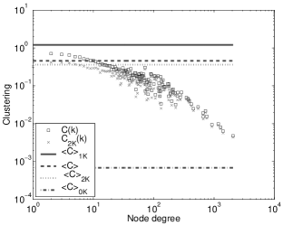
(a) skitter

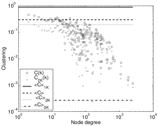
(b) BGP tables

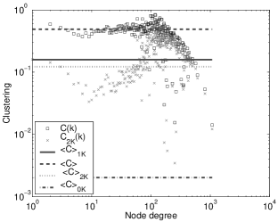
(c) WHOIS

Figure 14: Local clustering vs. graph randomness. Squares show local clustering observed in the real topology. The dashed line is its mean value. Crosses show local clustering predicted by the 2K-random graph model $C_{2K}(k)$. The dotted line is its mean value. The solid and dash-dotted lines are constant clusterings predicted by the 1K- and 0K-random graph models.

We compare clustering observed in our three Internet graphs with the predicted values for different graph models (Figure 14). In the skitter and BGP cases, the local clustering function $C_{2K}(k)$ calculated for the 2K-random model follows, albeit shifted down, the form of actually observed clustering $C(k)$. The ratio of corresponding mean values $\bar{C}_{2K}/\bar{C}$ is 0.8 for the skitter graph and 0.7 for the BGP graph. In the WHOIS case, the functional behavior of the model and of the observed clustering are different, and the ratio of their mean values is 0.25. We conclude that, using the metric of clustering, the skitter graph is closest to being 2K-random, while the WHOIS graph is the furthest. This finding has a direct impact on topology generators: it implies that the skitter topology can be successfully recreated by capturing the JDD observed in the measured topology. We surmise that a 2K-random generator will closely approximate the skitter graph. Similarly, a 2K-random generator reproducing the JDD observed in the measured BGP graph will be able to create an approximate model of the BGP graph.

Figure 14 also shows the constant values of local clustering predicted by the corresponding 1K- and 0K-random graph models, $C_{1K}$ (solid line) and $C_{0K}$ (dash-dotted line). Naturally, the 1K-random graphs, with a constant form of local clustering, less accurately describe the observed clustering than 2K-random model, except in the WHOIS case, which is closest to being 1K-random. Clustering in the 0K-random graphs is even further away, being orders of magnitude smaller than the clustering observed in all three graphs. Note that the ratio of $\bar{C}_{0K}/\bar{C}_{1K}$ is an indirect indicator of a graph’s proximity to being 0K-random. The $\bar{C}_{0K}/\bar{C}_{1K}$ values for our graphs ($1\cdot 10^{-2}$ for the WHOIS, $6\cdot 10^{-4}$ for the skitter, and $3\cdot 10^{-4}$ for the BGP) indicate that the WHOIS graph is better approximated by 0K-random model, compared with the other two graphs. The BGP graph is the least 0K-random in that respect.

In summary, the 2K-random graph model approximates the skitter topology best, while the PLRG generator is inferior for all the three graphs.

5 Limitations

Our work suffers from a number of methodological limitations and biases. We discuss each in turn below along with the potential consequences.

We have tried to be exhaustive while compiling our list of graph metrics considered by the community. However, it is possible that we may have missed important metrics or that additional important metrics may be proposed that are not well captured by, for instance, joint degree distribution.

Another limitation is our available data. Although the data sets we examine represent the current state of the art in macroscopic AS topology, they are incomplete and indirect reflections of the underlying topology. They require processing before producing the desired AS graph. For all our data sets, researchers must make choices while dealing with ambiguities and errors in the raw data. One such example is the detection of “false” links created by route changes in traceroute data. This paper does not address how different choices in processing the original data may result in different values for our target metrics. Instead we have attempted, where possible, to use best practices to extract topologies as presented in papers and in our discussions with other researchers.

Next, we limit our data collection to a single month for obtaining skitter and BGP data. While we believe that our results will hold true for historical data and are not an artifact of the current Internet or our sampling period, we leave this study to future work.

Finally, we come to the role played by JDD in topological studies. JDD has successfully explained the resulting metric values as well as inherent differences in skitter, BGP and WHOIS graphs. As a next step, we compare clustering in our observed topologies to the predicted clustering values in the 2K-random graph. The proximity between the observed and predicted models gives us further reason to believe that graphs generated by the 2K-random model come close to the original topology. Ideally, we could use a graph generator that uses the measured JDD of a graph to produce random graphs with similar JDDs, which in turn would also display similar values for a variety of important graph metrics. We leave such a potential demonstration of the value of JDD for capturing a broad range of graph characteristics to future work.

6 Analysis and Conclusions

We discussed the properties of Internet AS-level topologies extracted from the three most popular sources of AS topology data: skitter measurements, BGP tables, and the RIPE WHOIS database. We compared the derived topologies based on a set of important and frequently used statistical characteristics.

We further presented a detailed comparison of widely available sources of topology data in terms of a number of popular metrics studied in the literature. Of the set of metrics we considered, the joint degree distribution $P(k_{1},k_{2})$ embeds the most information about a graph, since this distribution determines both the average node degree $\bar{k}$ and the assortativity coefficient $r$. We find that, for the data sources we consider, a 2K-random model reproducing the JDD of the original topology also captures other crucial topological characteristics. While additional work is required to verify this claim, we believe that JDD may be a powerful metric for capturing a variety of important graph properties. Isolating such a metric or small set of metrics is a prerequisite to developing a accurate topology generators to assist a broad array of research and development efforts. Developing such a JDD-based topology generator and further demonstrating this concept is the subject of our current research.

We also propose criteria to evaluate how well the random graph models reproducing the average node degree $\bar{k}$ (0K-random), the degree distribution $P(k)$ (1K-random), or the JDD $P(k_{1},k_{2})$ (2K-random) approximate characteristics of the observed topologies. Using clustering as a measure of accuracy of the 2K-random approximation, we find that the 2K-random model describes the skitter graph most accurately. Using the assortativity coefficient (calculated from the JDD) as a measure of accuracy of the 1K-random approximation, we find that 1K- or 0K-random graph descriptions best fit the WHOIS graph, but are less successful in the skitter and BGP cases. The latter fact implies that the power law random graph (PLRG) model (which is a special case of 1K-random models) and topology generators based on it fail to accurately capture the important properties of the skitter or BGP graphs. Similarly, the PLRG model fails to recreate the WHOIS graph since its node degree distribution does not follow a power law at all.

Finally, one may ask which data source is closest to reality. We emphasize that there is not one but at least three data sources of the Internet AS-level topology: skitter, BGP, and WHOIS data, and that the resulting graphs present different views of the Internet. The skitter graph closely reflects the topology of actual Internet traffic flows, i.e. the data plane. The BGP graph reveals the topology seen by the routing system, i.e. the control plane. Naturally, these two topologies are somewhat different. Understanding their incongruities is a subject of ongoing research [51, 18, 52]. The WHOIS graph represents a record of the Internet topology created by human actions, i.e. the management plane. It is not surprising that this human-generated view of the Internet has different topological properties than the other two graphs. The observed abundance of tangential links between ASes is likely to reflect unintentional or even intentional over-reporting by some providers of their peering arrangements.

Our analysis should arm researchers with better insights into specifics of each topology. We hope that our study encourages the validation of existing models against real data and also motivates t he development of better topology models.

Table 3: Summary statistics.

		skitter	BGP tables	WHOIS
Average degree	Number of nodes $(n)$	9,204	17,446	7,485
	Number of edges $(m)$	28,959	40,805	56,949
	Avg node degree $(\bar{k})$	6.29	4.68	15.22
Degree distr	Max node degree $(k_{max})$	2,070	2,498	1,079
	Power-law max degree $(k_{max}^{PL})$	1,448	4,546	-
	Exponent of $P(k)\;(-\gamma)$	2.25	2.16	-
Joint degree distr	Avg neighbor degree $(\bar{k}_{nn}/(n-1))$	0.05	0.03	0.02
	Exponent of $k_{nn}(k)\;(-\gamma_{nn})$	1.49	1.45	-
	Assortative coefficient $(r)$	-0.24	-0.19	-0.04
Clustering	Mean clustering $(\bar{C})$	0.46	0.29	0.49
	Clustering coefficient $(C)$	0.03	0.02	0.31
	Exponent of $C(k)\;(-\gamma_{C})$	0.33	0.34	-
Rich club	Exponent of $\phi(\rho/n)\;(-\gamma_{rc})$	1.48	1.45	1.69
Coreness	Avg node coreness $(\bar{\kappa})$	2.23	1.41	7.65
	Max node coreness $(\kappa_{max})$	27	27	87
	Core size ratio $(n_{core}/n)$	$5\cdot 10^{-3}$	$3\cdot 10^{-3}$	$17\cdot 10^{-3}$
	Min degree in core $(k_{core}^{min})$	68	34	99
	Fringe size ratio $(n_{fringe}/n)$	0.27	0.29	0.06
	Max degree in fringe $(k_{fringe}^{max})$	5	7	4
	Exponent of $\kappa(k)\;(\gamma_{\kappa})$	0.68	0.58	1.07
Distance	Avg distance $(\bar{d})$	3.12	3.69	3.54
	Std deviation of distance $(\sigma)$	0.63	0.87	0.80
	Exponent of $d(k)\;(-\gamma_{d})$	0.07	0.07	0.09
Eccentricity	Graph radius $(R,\;\varepsilon_{min})$	4	5	4
	Avg eccentricity $(\bar{\varepsilon})$	5.11	6.61	6.12
	Graph diameter $(D,\;\varepsilon_{max})$	7	10	8
	Center size ratio $(n_{R}/n)$	$320\cdot 10^{-4}$	$14\cdot 10^{-4}$	$1\cdot 10^{-4}$
	Min degree in center $(k_{R}^{min})$	4	188	1,079
	Periphery size ratio $(n_{D}/n)$	$21\cdot 10^{-4}$	$2\cdot 10^{-4}$	$106\cdot 10^{-4}$
	Max degree in periphery $(k_{D}^{max})$	1	1	6
Betweenness	Avg node betweenness $(\bar{B}_{node}/(n(n-1)))$	$11\cdot 10^{-5}$	$7.7\cdot 10^{-5}$	$17\cdot 10^{-5}$
	Exponent of $B(k)\;(\gamma_{B})$	1.35	1.17	-
	Avg edge betweeness $(\bar{B}_{edge}/(n(n-1)))$	$5.37\cdot 10^{-5}$	$4.51\cdot 10^{-5}$	$3.10\cdot 10^{-5}$
Spectrum	Largest eigenvalue	79.53	73.06	150.86
	Second largest eigenvalue	-53.32	-55.13	68.63
	Third largest eigenvalue	36.40	53.54	62.03

7 Acknowledgments

We thank Ulrik Brandes for sharing his betweenness code with us and Andre Broido for answering our questions.

Support for this work was provided by NSF CNS-0434996, NCS ANI-0221172, Cisco’s University Research program, and other CAIDA members.

References

- [1] M. Faloutsos, P. Faloutsos, and C. Faloutsos, “On power-law relationships of the Internet topology,” in ACM SIGCOMM, 1999, pp. 251–262.
- [2] Q. Chen, H. Chang, R. Govindan, S. Jamin, S. J. Shenker, and W. Willinger, “The origin of power laws in Internet topologies revisited,” in IEEE INFOCOM, 2002.
- [3] H. Tangmunarunkit, R. Govindan, S. Jamin, S. Shenker, and W. Willinger, “Network topology generators: Degree-based vs. structural,” in ACM SIGCOMM, 2002, pp. 147–159.
- [4] L. Li, D. Alderson, W. Willinger, and J. Doyle, “A first-principles approach to understanding the Internet s router-level topology,” in ACM SIGCOMM, 2004.
- [5] T. Bu and D. Towsley, “On distinguishing between Internet power law topology generators,” in IEEE INFOCOM, 2002.
- [6] S. Jaiswal, A. L. Rosenberg, and D. Towsley, “Comparing the structure of power-law graphs and the Internet AS graph,” in IEEE ICNP, 2004.
- [7] M. Gaertler and M. Patrignani, “Dynamic analysis of the Autonomous System graph,” in IPS, 2004.
- [8] S. Zhou and R. J. Mondragón, “Accurately modeling the Internet topology,” Physical Review E, vol. 70, pp. 066108, 2004, http://arxiv.org/abs/cs.NI/0402011.
- [9] S. N. Dorogovtsev and J. F. F. Mendes, Evolution of Networks: From Biological Nets to the Internet and WWW, Oxford University Press, Oxford, 2003.
- [10] CAIDA, “Toward mathematically rigorous next-generation routing protocols for realistic network topologies,” Research Project, http://www.caida.org/projects/nets-nr/.
- [11] A. Vahdat, K. Yocum, K. Walsh, P. Mahadevan, D. Kostic, J. Chase, and D. Becker, “Scalability and accuracy in a large-scale network emulator,” in OSDI, 2002.
- [12] kc claffy, T. E. Monk, and D. McRobb, “Internet tomography,” Nature, January 1999, http://www.caida.org/tools/measurement/skitter/.
- [13] “University of Oregon RouteViews Project,” http://www.routeviews.org/.
- [14] “Internet Routing Registries,” http://www.irr.net/.
- [15] CAIDA, “Comparative analysis of the Internet AS-level topologies extracted from different data sources: Data page,” http://www.caida.org/analysis/topology/as_topo_comparisons/.
- [16] “traceroute,” http://www.traceroute.org/#source%20code.
- [17] CAIDA, “Macroscopic topology AS adjacencies,” http://www.caida.org/tools/measurement/skitter/as_adjacencies.xml.
- [18] Z. M. Mao, J. Rexford, J. Wang, and R. H. Katz, “Towards an accurate AS -level traceroute tool,” in ACM SIGCOMM, 2003.
- [19] Y. Rekhter and T. Li, A Border Gateway Protocol 4 (BGP-4), IETF, RFC 1771, 1995.
- [20] J. Hawkinson and T. Bates, Guidelines for Creation, Selection, and Registration of an Autonomous System (AS), IETF, RFC 1930, 1996.
- [21] G. Siganos and M. Faloutsos, “Analyzing BGP policies: Methodology and tool,” in IEEE INFOCOM, 2004.
- [22] H. Chang, R. Govindan, S. Jamin, S. J. Shenker, and W. Willinger, “Towards capturing representative AS-level Internet topologies,” Computer Networks Journal, vol. 44, pp. 737–755, April 2004.
- [23] CAIDA, “Visualizing Internet topology at a macroscopic scale,” http://www.caida.org/analysis/topology/as_core_network/.
- [24] A. Lakhina, J. Byers, M. Crovella, and P. Xie, “Sampling biases in IP topology measurements,” in IEEE INFOCOM, 2003.
- [25] L. Dall’Asta, I. Alvarez-Hamelin, A. Barrat, A. Vázquez, and A. Vespignani, “Exploring networks with traceroute-like probes: Theory and simulations,” Theoretical Computer Science, Special Issue on Complex Networks, 2005, http://arxiv.org/abs/cs.NI/0412007.
- [26] CAIDA, “Automated Autonomous System (AS) ranking,” Research Project, http://www.caida.org/analysis/topology/rank_as/.
- [27] M. E. J. Newman, “Assortative mixing in networks,” Physical Review Letters, vol. 89, no. 20, pp. 208701, 2002.
- [28] S. N. Dorogovtsev, “Networks with given correlations,” http://arxiv.org/abs/cond-mat/0308336v1.
- [29] J. Winick and S. Jamin, “Inet-3.0: Internet topology generator,” Technical Report UM-CSE-TR-456-02, University of Michigan, 2002.
- [30] Y. Breitbart, C.-Y. Chan, M. Garofalakis, R. Rastogi, and A. Silberschatz, “Efficiently monitoring bandwidth and latency in IP networks,” in IEEE INFOCOM, 2001.
- [31] K. Park and H. Lee, “On the effectiveness of route-based packet filtering for distributed DoS attack prevention in power-law internets,” in ACM SIGCOMM, 2001.
- [32] B. Bollobás and O. Riordan, “Mathematical results on scale-free random graphs,” in Handbook of Graphs and Networks, Berlin, 2002, Wiley-VCH.
- [33] M. E. J. Newman, “Properties of highly clustered networks,” Physical Review E, vol. 68, pp. 026121, 2003.
- [34] P. Fraigniaud, “A new perspective on the small-world phenomenon: Greedy routing in tree-decomposed graphs,” Technical Report LRI-1397, LRI, University Paris-Sud, 2005.
- [35] S. N. Soffer and A. Vázquez, “Clustering coefficient without degree correlations biases,” http://arxiv.org/abs/cond-mat/0409686.
- [36] B. Bollobás, Random Graphs, Academic Press, New York, 1985.
- [37] F. Harary, Graph Theory, Addison-Wesley, Reading, MA, 1994.
- [38] I. Alvarez-Hamelin, L. Dall’Asta, A. Barrat, and A. Vespignani, “-core decomposition: A tool for the visualization of large scale networks,” http://arxiv.org/abs/cs.NI/0504107.
- [39] D. Peleg, Distributed Computing: A Locality-Sensitive Approach, SIAM, Philadelphia, PA, 2000.
- [40] D. Krioukov, K. Fall, and X. Yang, “Compact routing on Internet-like graphs,” in IEEE INFOCOM, 2004.
- [41] U. Brandes, “A faster algorithm for betweenness centrality,” Journal of Mathematical Sociology, vol. 25, no. 2, pp. 163–177, 2001.
- [42] F. K. R. Chung, Spectral Graph Theory, vol. 92 of Regional Conference Series in Mathematics, American Mathematical Society, Providence, RI, 1997.
- [43] C. Gkantsidis, M. Mihail, and A. Saberi, “Conductance and congestion in power law graphs,” in ACM SIGMETRICS, 2003.
- [44] D. Vukadinović, P. Huang, and T. Erlebach, “A spectral analysis of the Internet topology,” Technical Report TIK-NR. 118, ETH, 2001.
- [45] C. Gkantsidis, M. Mihail, and E. Zegura, “Spectral analysis of Internet topologies,” in IEEE INFOCOM, 2003.
- [46] P. Erdős and A. Rényi, “On random graphs,” Publicationes Mathematicae, vol. 6, pp. 290–297, 1959.
- [47] M. Molloy and B. Reed, “A critical point for random graphs with a given degree sequence,” Random Structures and Algorithms, vol. 6, pp. 161–179, 1995.
- [48] M. Molloy and B. Reed, “The size of the giant component of a random graph with a given degree sequence,” Combinatorics, Probability and Computing, vol. 7, pp. 295–305, 1998.
- [49] W. Aiello, F. Chung, and L. Lu, “A random graph model for massive graphs,” in Proceedings of the 32nd Annual ACM Symposium on Theory of Computing (STOC). 2000, pp. 171–180, ACM Press.
- [50] S. N. Dorogovtsev, “Clustering of correlated networks,” Physical Review E, vol. 69, pp. 027104, 2004.
- [51] Y. Hyun, A. Broido, and kc claffy, “Traceroute and BGP AS path incongruities,” in Cooperative Association for Internet Data Analysis (CAIDA), 2003, http://www.caida.org/outreach/papers/2003/ASP/.
- [52] Z. M. Mao, D. Johnson, J. Rexford, J. Wang, and R. Katz, “Scalable and accurate identification of AS-level forwarding paths,” in IEEE INFOCOM, 2004.