Truth-telling Reservations

Abstract

We present a mechanism for reservations of bursty resources that is both truthful and robust. It consists of option contracts whose pricing structure induces users to reveal the true likelihoods that they will purchase a given resource. Users are also allowed to adjust their options as their likelihood changes. This scheme helps users save cost and the providers to plan ahead so as to reduce the risk of under-utilization and overbooking. The mechanism extracts revenue similar to that of a monopoly provider practicing temporal pricing discrimination with a user population whose preference distribution is known in advance.

1 Introduction

A number of compute intensive applications often suffer from bursty usage patterns [1, 3, 5, 6, 9], whereby the demand for IT, memory and bandwidth resources can at times exceed the installed capacity within the organization. This problem can be addressed by providers of IT services who satisfy this peak demand for a given price, playing a role similar to utilities such as electricity or natural gas.

The emergence of a utility form of IT provisioning creates in turn a number of problems for both providers and customers due to the uncertain nature of IT usage. On the provider side there is a need to design appropriate pricing schemes to encourage the use of such IT services and to gain better estimates of the usage pattern so as to enable effective statistical multiplexing. On the customer side, there needs to be a simple way of figuring out how to anticipate and hedge the need for uncertain demand as well as the costs that it will add to the overall IT operations.

Recently, it was proposed to use swing options for pricing the reservation of IT resources [3]. By purchasing a swing option the user pays an upfront premium to acquire the right, but not the obligation, to use a resource as defined in the option contract. As with the case with electricity, IT resources, such as bandwidth and CPU time, are non-storable and with volatile usage pattern. Thus, swing options provide flexibility in both the amount and the time period for which a resource is purchased, making them appealing to users whose bursty demand is hard to predict. From the point of view of the providers, if enough users purchase these options providers can offset the cost of providing peak capacity by multiplexing among many users.

Pricing a swing option for IT resources however, turns out to be difficult because of the complexity of the option contract and the lack of a good model of the spot market price, which at present is nonexistent. Moreover, there are two important problems that need resolution. First, the user needs to be able to estimate the amount of resources that need to be reserved as well as their cost; and second, the provider needs to put in place a mechanism that will induce truth revelation on the part of the user when stating the likelihood that a given reservation or option will be exercised.

As was shown in [3], the first problem can be addressed by providing the user with a simulation tool for estimating the cost of a reservation from a set of historical data, as well as a provision for entering the user’s assumptions about aggressive or conservative swings. Because the prices for swings are set ahead of time and not by market forces, the forecasting tool also provides a powerful “what-if” capability to both the resource provider and the customer for estimating outright costs and risks associated with fluctuations in customer demand.

As to the provider’s problem with asymmetric information, it could be argued that a user’s historical usage pattern allows to predict his future demand. But in many cases, such as with new users, the data may not be available or reflect unanticipated user needs. Even worse, users may misrepresent the likelihood of their needs in order to gain a pricing advantage, with the consequent loss to the provider. In the original design of the swing option this was addressed by introducing a time dependent discount that induces early commitment to a contract. But this strategy still allows users to misrepresent their likelihoods the first time they buy an option.

This paper presents a solution to the truth revelation problem in reservations by designing option contracts with a pricing structure that induces users to reveal their true likelihoods that they will purchase a given resource. A user is allowed to adjust his option later if his likelihood changes. Truthful revelation helps the provider to plan ahead to reduce the risk of under-utilization and overbooking, and also helps the users to save cost. In addition to its truthfulness and robustness, the mechanism extracts revenue similar to that of a monopoly provider monopoly provider practicing temporal pricing discrimination with a user population whose preference distribution is known in advance [2, 4, 5, 7, 8, 9, 10].

We start by presenting a simple two period model in which at the first period the user knows his probability of using the resource at the second period and purchases a reservation whose price depends on that probability. A coordinator then aggregates the reservations from all users and purchases the needed resources from the provider. These resources are then purchased in the second period. A nonlinear pricing scheme is shown to lead to both truthful revelation and profitability to both users and coordinator.

We then extend the two period model to a multi period model which allows the user’s likelihoods of use to change over time. In this more realistic scheme, users are allowed adjust their options according to updated information about their needs while remaining truthful at each time period.

Finally we show how this truth-telling reservation mechanism can be interpreted in terms of standard options terminology, and finish with a discussion of the feasibility of this mechanism to provide revenues to both users and providers.

While the focus of this paper is on reservations for IT resources, there are many other interesting situations where our mechanism can be useful. For example, conference rooms in many organizations tend to be reserved in advance in the likelihood that they will be needed for future meetings. The resulting behavior leads to serious inefficiencies through reservations that are not exercised and which force others to reschedule important meetings. A truth telling mechanism like the one we propose would lead to a more efficient scheduling of such conferences. Likewise, airline seats, hotel reservations, network bandwidth and tickets for popular shows would benefit from a properly priced reservation system, leading to both more predictable use and revenue generation.

2 The Two Period Model

Consider $n$ users $\{1,2,\dots,n\}$ who live for two discrete periods. Each user may need have to consume one unit of resource in period 2, which he can buy from a resource provider either in period 1 at a discount price $1$, or in period 2 at a higher price $C>1$. In period 1, each user $i$ only knows the probability $p_{i}$ that he will need the resource in the next period. It is not until period 2 that he can be certain about his need (unless $p=0$ or $1$). We also assume that the distributions of the users’ needs are independent.

Suppose all the users wish to pay the least while behaving in a risk-neutral fashion. User $i$ can either pay $1$ in period 1, or wait until period 2 and pay $C$ if it turns out he has to, an event that happens with probability $p_{i}$. Obviously, he will use the former strategy when $Cp_{i}>1$ and the latter strategy when $Cp_{i}<1$, while his cost is $\min(1,Cp_{i})$.

This optimal paying plan can be very costly for the user. For example, when $C=5$ and $p=0.1$, the user always postpones the decision to buy until period 2, ending up paying $5$ for every unit he needs.

In what follows we describe a reservation mechanism that allows him to pay a small premium that guarantees his one unit of resource whenever he needs it in period 2, at a price not much higher than the discount price $1$. In addition, the mechanism makes the user truthfully reveal his probability of using the resource to the provider, who can then accurately anticipate user demand. At a later stage, we show how this mechanism can be thought of as an option.

2.1 The coordinator game

To better illustrate the benefit of this mechanism, we introduce a third agent, the coordinator, who aggregates the users’ probabilities and makes a profit while absorbing the users’ risk. He does so in a two period game, which we now describe.

1. (Period 1) The coordinator asks each user to submit a probability $q_{i}$, which does not have to be the real probability $p_{i}$ that the user will need one unit of resource in period 2.

2. (Period 1) The coordinator reserves $\sum q_{i}$ units of resource from the resource provider (at the discount price), ready to be consumed in period 2.

3. (Period 2) The coordinator delivers the reserved resource units to users who claim them. If the amount he reserved is not enough to satisfy the demand, he buys more resource from the provider (at the higher unit price $C$) to meet the demand.

4. (Period 2) User $i$ pays

   $$\begin{cases}f(q_{i})&\text{if he needs one unit of resource,}\\ g(q_{i})&\text{if he does not need it,}\end{cases}$$ (1)

   where $f,g:[0,1]\to\mathbb{R}^{+}$ are two functions whose forms will be specified later.

These terms are completely transparent to everyone, before step 1.

For the coordinator to profit, the following two conditions have to be satisfied:

Condition A.

The coordinator can make a profit by providing this service.

Condition B.

Each user prefers to use the service provided by the coordinator, rather than to deal with the resource provider directly.

The next two truth-telling conditions, although not absolutely necessary, are useful for conditions A and B to hold.

Condition T1.

(Step 1 truth-telling) Each user submits his true probability $p_{i}$ in step 1, so that he expects to pay the least later in step 4.

Condition T2.

(Step 3 truth-telling) In step 3, when a user does not need a resource in period 2, he reports it to the coordinator.

From Condition T1. User $i$ expects to pay

$$w(q_{i})\equiv p_{i}f(q_{i})+(1-p_{i})g(q_{i})$$ (2)

in period 2. His optimal submission $q_{i}^{*}$ is determined by the first-order condition

$$w^{\prime}(q_{i}^{*})=p_{i}f^{\prime}(q_{i}^{*})+(1-p_{i})g^{\prime}(q_{i}^{*})=0.$$ (3)

Truth-telling requires that $q_{i}^{*}=p_{i}$, or

$$p_{i}f^{\prime}(p_{i})+(1-p_{i})g^{\prime}(p_{i})=0.$$ (4)

Condition T2 simply requires that

$$f(p)\geq g(p)\quad\text{for all }p\in[0,1].$$ (5)

Now we study Condition A when all users submit their true probabilities $\{p_{i}\}$. Let $U$ be the total resource usage of all users in period 2, and let $W$ be the their total payment. Both $U$ and $W$ are random variables. Clearly,

$$\mathbb{E}\,U=\sum p_{i},$$ (6)

and

$$\mathbb{E}\,W=\sum w(p_{i}).$$ (7)

Lemma 1.

If there exists an arbitrarily small $\epsilon>0$ such that

$$w(p)\geq p+\epsilon\quad\text{for all }p\in[0,1],$$ (8)

then

$$W-U\to\infty\text{ a.s. \quad as }n\to\infty,$$ (9)

i.e. by charging an arbitrarily small premium, the coordinator makes profit when there are many users (Condition A).

Proof. This follows directly from the “$X^{4}$-strong law”. (See e.g. David Willams, Probability with Martingales, pp. 72–73, Cambridge University Press, 2001. The random usage of each user does not have to be identically distributed.) $\Box$

The small number $\epsilon$ is merely a technical device. In what follows we will neglect it and use a weakened version of Eq. (8) as a sufficient condition of Condition A (not rigorous):

$$w(p)\geq p\quad\text{for all }p\in[0,1].$$ (10)

Last, Condition B says that the user can save money by using the coordinator’s service:

$$w(p)\leq\min(1,Cp)\quad\text{for all }p\in[0,1].$$ (11)

To summarize, the following conditions on $f$ and $g$ are sufficient for the truth-telling mechanism to work:

$$pf^{\prime}(p)+(1-p)g^{\prime}(p)=0,$$ (12)

$$f(p)\geq g(p),$$ (13)

$$p\leq pf(p)+(1-p)g(p)\leq\min(1,Cp),$$ (14)

for all $p\in[0,1]$.

Consider the following choice:

$$f^{\prime}(p)=-k(1-p),\quad g^{\prime}(p)=kp,$$ (15)

which obviously satisfies Eq. (12). Letting $p=0$ and 1 in Eq. (14) gives two boundary conditions for $f$ and $g$:

$$f(1)=1,\quad g(0)=0.$$ (16)

The solution for Eq. (15) and (16) is

$$f(p) = 1+\frac{k}{2}-kp+\frac{kp^{2}}{2},$$ (17)

$$g(p) = \frac{kp^{2}}{2}.$$ (18)

To check Eq. (13) and (14), we first calculate

$$w(p)=\left(1+\frac{k}{2}\right)p-\frac{k}{2}p^{2}.$$ (19)

And then it is not hard to show

Lemma 2.

For the choice of $f$ and $g$ in Eq. (17) and (18), conditions (13) and (14) are satisfied for $k\in[1,\min\{2(C-1),2\}]$.

Proof. Eq. (13) is satisfied because

$$f(p)-g(p)=1+k\left(\frac{1}{2}-p\right)\geq 1-\frac{k}{2}\geq 0.$$ (20)

To verify Eq. (14), we write

$$w(p) = p+\frac{k}{2}p(1-p)\geq p,$$ (21)

$$w(p) = 1-(1-p)\left(1-\frac{k}{2}p\right)\leq 1,$$ (22)

$$w(p) \leq Cp-\frac{k}{2}p^{2}\leq Cp.$$ (23)

$\Box$

\psfrag{p}{{\color[rgb]{0,0,1}$p$}}\psfrag{w}{{\color[rgb]{1,0,0}$w(p)$}}\psfrag{min}{{\color[rgb]{0,0,1}$\min(1,Cp)$}}\psfrag{pp}{$p$}\includegraphics[scale={.7}]{w.eps}

Figure 1: Plot of $w(p)$ for $C=2$ and $k=1.5$. The red curve $w(p)$ lies completely in the region enclosed by the two blue curves.

Fig. 1 shows the special case $C=2$ and $k=1.5$. As can be seen, the red curve $w(p)$ lies completely between the two blue curves. The difference between the upper blue curve and the red curve is the amount of money the user saves (varying with different $p$). The difference between the red curve and the lower blue line is the coordinator’s expected payoff from one user. Note that his payoff is larger for values of $p$’s lying in the middle of the range, and is zero for $p=0$ and $p=1$. This result is hardly surprising, for when there is no uncertainty the user does not need a coordinator at all. Thus, the coordinator makes a profit out of uncertainties in user behavior.

\psfrag{p}{$p$}\psfrag{f}{{\color[rgb]{1,0,0}$f(p)$}}\psfrag{g}{{\color[rgb]{0,0,1}$g(p)$}}\includegraphics[scale={.7}]{fg.eps}

Figure 2: Payment curves of the user for $C=2$ and $k=1.5$. If the user needs one unit of resource in period 2, he pays according to the upper curve. Otherwise he pays according to the lower curve.

Fig. 2 plots the two payment curves, $f(p)$ and $g(p)$, for $C=2$ and $k=1.5$. After signing a contract, a user agrees to pay later either the upper curve for one unit of resource, or the lower curve for nothing. Note that $f(p)$ is strictly decreasing, a feature essential for the user to be truth-telling. A user with a high $p$ is more likely to pay the upper curve rather than the lower curve. Knowing this, he has an incentive to submit a high probability of use and thus not to cheat.

2.2 The reservation contract as an option

The contract discussed in previous sections can be equivalently regarded as an “option”. Because $g(p)$ is the minimal amount the user has to pay in any event, we can ask him to pay it in period 1, and only to pay $f(p)-g(p)$ in period 2 if he needs one unit of resource at that time. Hence, by paying an amount $g(p)$, the user achieves the right but no the obligation to buy one unit of resource at price $f(p)-g(p)$ in period 2. Naturally, we may call $g(p)$ the premium or the price of option, and $f(p)-g(p)$ the price of the resource.

\psfrag{fg}{$f(p)-g(p)$}\psfrag{g}{$g(p)$}\includegraphics[scale={.7}]{curve.eps}

Figure 3: Price-premium curve for the user. The horizontal axis is the premium (value of contract, value of option). The vertical axis is the price the user pays for one unit of resource in period 2.

Fig. 3 shows the parametric plot of resource price versus option price, for $p\in[0,1]$. Instead of submitting an explicit $p$, the user can equivalently choose one point on this curve and pay accordingly. His probability $p$ can then be inferred from his choice (using Eq. (17) or (18)). This alternative method may be more user-friendly because people tend to be more sensitive to monetary values rather than probabilities. We can even further simplify the curve by providing the user with a table with the values of a few discrete points along the curve.

2.3 Possible extensions

Simple as it may seem, the two period model can already solve a wide range of reservation problems. Here we show how the mechanism can be extended to solve more nontrivial problems, as when there is uncertainty not only in the consumption of one unit, but also in both the number of consumption units and their consumption time.

Example 1.

(Uncertain number of units) By checking past web statistics, a company discovers that its website has the following pattern of visits: 90% of the days it needs one unit of bandwidth, 6% of the days two units, 3% of the days three units, only 1% of the days does it need four units of bandwidth.

Here the company faces a four-point distribution of usage rather than a two-point distribution (either 1 or 0) discussed in the two period model. Imagine there are four units of resources: $U_{1}$, $U_{2}$, $U_{3}$ and $U_{4}$. The company’s usage pattern can be written as $P(U_{1})=0.9$, $P(U_{1}U_{2})=0.06$, $P(U_{1}U_{2}U_{3})=0.03$, and $P(U_{1}U_{2}U_{3}U_{4})=0.01$. Breaking down to individual unit, the pattern is $P(U_{1})=1$ (for sure one unit will be consumed), $P(U_{2})=0.1$ (with probability 0.1 the company will need at least two units), $P(U_{3})=0.04$, and $P(U_{4})=0.01$. Thus, to efficiently reserve bandwidth for some day in the future, the company can reserve one unit for sure, and buy three options, all for the same day, with $p=0.1$, 0.04, and 0.01 respectively.

Example 2.

(Uncertain consumption time) A biochemist will need for sure to use a public supercomputer to run some CPU-heavy simulations next month, but he has no idea on which day he will need it. He wants to reserve the supercomputer now to save cost.

Say that the next month has 30 days. The probability that he will need the computer on one particular day next month is $p=1/30$. He can buy 30 “$p=1/30$” options, one for each day next month. For a numerical calculation, assume that $C>2$ and $k=2$. His total expected cost would then be

$$30\,g(\frac{1}{30})+f(\frac{1}{30})-g(\frac{1}{30})=2-\frac{1}{30}\approx 2,$$ (24)

so he pays less than 2 for an uncertainty over 30 days, which is not bad.

Remark: The careful reader might notice that in Example 1, the $U_{i}$’s are no longer independent, whereas in Example 2, the consumptions on two different days are not independent either. This is not really a problem, because although the options reserved by one user can be dependent, as long as the options reserved by different users are independent, Lemma 1 still works.

3 A Multi Period Truth-Telling Reservation

In the previous 2-period mechanism, if a user learns more in time about the likelihood of his needing the resource, it is impossible for him to modify the original contract. To solve this issue we extend our mechanism so that the user can both submit early for a larger discount and update his probability afterwards to a more accurate one. We thus consider a dynamic extension of the problem in which the user is allowed to change his probability of future use some time after his initial submission.

3.1 The information structure

Assume that everyone lives for three periods. In period 3 the user might need to consume one unit of resource. He can either reserve one unit in period 1 at price 1, or in period 2 at a price $C>1$, or buy it in period 3 at price $C^{2}$. The additional period 2 is introduced to exploit the user’s information gaining process. In order to make this meaningful we need to carefully define the information structure, especially what does “gain more information” mean.

Suppose that each user can end up in either state $A$ or state $B$ in period 2. When in period 1, the user knows his probability of entering each of the two states ($A$ or $B$), but he does not know exactly which state he will enter until after period 2. In this sense, we say that the user “gains” an extra bit of “state information” in period 2. His probability of consuming one unit of resource in period 3 actually depends on his state and will thus report a more accurate probability once he gets the “state information”.

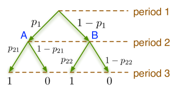
Figure 4: The information structure for three periods.

This information structure is depicted in Fig. 4. The user enters state $A$ with probability $p_{1}$ and state $B$ with probability $1-p_{1}$. If he enters state $A$, with probability $p_{21}$ he will need the resource in period 3. If he enters state $B$, he will need the resource with probability $p_{22}$. He knows these probabilities $(p_{1},p_{21},p_{22})$ at the beginning. Clearly, in period 1 when he has no state information, his probability of needing the resource in period 3 is

$$p=p_{1}p_{21}+(1-p_{1})p_{22}.$$ (25)

Example 3.

On New Year’s day, a user is struggling against a paper deadline due on Feb 1, which is for a conference to be held on Apr 1. With probability 0.7 he will finish the paper before the deadline, and there is 0.6 probability that it will get accepted. If he cannot finish it before the deadline, he can still submit a post-deadline paper, which will only be accepted with probability 0.2. He will be informed whether his paper is accepted some time after his submission. He is thinking of booking a plane ticket now.

The three periods are Jan 1, Feb 1 and Apr 1. The probabilities are $p_{1}=0.7$, $p_{21}=0.6$, and $p_{22}=0.2$.

Remark: We should distinguish between the concepts of error and uncertainty. For example, by repeatedly tossing an unfair coin we can estimate its probability more and more accurately, but even if we know its exact probability distribution we still do not know what the outcome would be for the next time. That is, by maintaining a large history we can reduce error but not uncertainty. In our information structure we assume that the user knows his accurate probabilities (no error). In this context information is defined in the “uncertainty elimination” sense, rather than in the “error elimination” sense.

3.2 The three period coordinator game

Again we describe a mechanism used by a coordinator to make profit by aggregating the user’s uncertainty. A user may submit a probability in period 1, as in the 2-period setting. Additionally, when he enters period 2 he is allowed to update his probability based on his new information gained at that time. This way the user can enjoy the full discount while simultaneously utiize maximum information. His final payment in period 3 is determined by the one or two probabilities he submitted. The whole mechanism is described more rigorously as follows.

1. (Period 1) The user may submit a probability $q_{1}$, which is suggested but not obligatory to be the real probability $p=p_{1}p_{21}+(1-p_{1})p_{22}$ that he will need one unit of resource in period 3.

2. (Period 1) The coordinator reserves $q_{1}$ units of resource from the resource provider (at price 1).

3. (Period 2) The user may submit a probability $q_{2}$, which is suggested but not obligatory to be the real probability that he will need one unit of resource in period 3, based on his information at this time (i.e. either $p_{21}$ or $p_{22}$).

4. (Period 2) The coordinator adjusts his holdings to match the new probability $q_{2}$.

5. (Period 3) If the user claims the need of one unit of resource, the coordinator delivers one reserved unit to him. If his reservation pool is not large enough, he buys more resource from the provider (at the higher unit price $C^{2}$) to meet the demand.

6. (Period 3) The user pays according to Table 1:

   	$q_{1}$ not $q_{2}$	$q_{2}$ not $q_{1}$	both $q_{1}$ and $q_{2}$
   uses one unit	$f_{1}(q_{1})$	$f_{2}(q_{2})$	$f_{1}(q_{1})-\alpha f_{2}(q_{1})+\alpha f_{2}(q_{2})$
   does not use	$g_{1}(q_{1})$	$g_{2}(q_{2})$	$g_{1}(q_{1})-\alpha g_{2}(q_{1})+\alpha g_{2}(q_{2})$

   Table 1: The user’s payment table. The columns represent his three possible submission patterns.

In Table 1, $(f_{1},g_{1})$ and $(f_{2},g_{2})$ are two sets of 2-period truth-telling functions solved in Section 2.1.

$$f_{1}(p) = 1+\frac{k_{1}}{2}-k_{1}p+\frac{k_{1}p^{2}}{2},$$ (26)

$$g_{1}(p) = \frac{k_{1}p^{2}}{2},$$ (27)

$$f_{2}(p) = C+\frac{k_{2}}{2}-k_{2}p+\frac{k_{2}p^{2}}{2},$$ (28)

$$g_{2}(p) = \frac{k_{2}p^{2}}{2},$$ (29)

where $k_{1}\in[1,\min\{2(C^{2}-1),2\}]$ and $k_{2}\in[C,\min\{2(C^{2}-C),2C\}]$. To make the mathematical analysis easier, we will choose $k_{1}=k\in[1,\min\{2(C-1),2\}]$ and $k_{2}=Ck\in[C,\min\{2(C^{2}-C),2C\}]$, so that

$$f_{2}(p) = Cf_{1}(p),$$ (30)

$$g_{2}(p) = Cg_{1}(p).$$ (31)

We require that $f_{2}>f_{1}$ and $g_{2}>g_{1}$, so that the user pays more when he reserves late.

The third column of Table 1 needs special notice. The new parameter $\alpha>0$ is a “friction parameter” crucial for our mechanism to work. The expression $f_{1}(q_{1})-\alpha f_{2}(q_{1})+\alpha f_{2}(q_{2})$ can be understood as follows. First, the user signs a contract in period 1 and agrees to pay $f_{1}(q_{1})$ if he uses one unit of resource later. Second, in period 2 the user can adjust his probability to $q_{2}$ by “selling” some of his old $q_{1}$ contracts and “buying” some new $q_{2}$ contracts. Because he “sells” and “buys” in period 2, the selling and buying prices should be those of period 2, namely the two $f_{2}$ terms. We emphasize that in the contract form solution described here, the user only signs one contract that takes care of two periods and does not do any trading. However, there is an equivalent option formulation in which the user does sell his options, which we describe in Section 3.3.

Intuitively, because $f_{2}>f_{1}$, $\alpha$ has to be small enough since otherwise the users would want to “buy” a lot of $q_{1}$ contracts in period 1 and “sell” them later in period 2. In fact, it can be shown that there exists a nonempty region of $\alpha$ that allows the mechanism to work - that is, the user can save cost (even more than using the 2-period mechanism) and the coordinator can still profit. Formally, we have

Theorem 1.

Suppose $\alpha\in(0,1/C)$. The user’s optimal strategy is to submit a probability in period 1 and to adjust it in period 2. Each probability he submits is his true probability in that period. In addition, the coordinator is profitable.

Proof. Follows from Lemmas 3, 4, 5, and 6 in the Appendix. $\Box$

3.3 Three period options

As for the 2-period problem, there is an equivalent “option” form of the 3-period contract, which we now describe. Assume Eq. (30) and (31).

1. (Period 1) There are various options that the user can buy, with option price $g_{1}(p)$ and resource price $f_{1}(p)-g_{1}(p)$, for all $p\in[0,1]$. The user buys one share of $q_{1}$-option at price $g_{1}(q_{1})$.

2. (Period 2) The user can swap $\alpha C$ (remember $\alpha C<1$) share of his $q_{1}$-option for a $q_{2}$-option, by paying the difference price $\alpha C(g_{1}(q_{2})-g_{1}(q_{1}))$. Then he holds a share $(1-\alpha C)$ of $q_{1}$-options and a share $\alpha C$ of $q_{2}$-options.

3. (Period 3) If the user needs one unit of resource, he executes his options. That is, he pays $(1-\alpha C)(f_{1}(q_{1})-g_{1}(q_{1}))$ using his $q_{1}$ option, plus $\alpha C(f_{1}(q_{2})-g_{1}(q_{2}))$ using his $q_{2}$ option.

It is easy to verify that this option payment plan is equivalent to Table 1.

Remarks:

1. In period 2 when the user swaps part of his option, he does this at no additional cost.

2. In the plan discussed above all options are issued in period 1. There can be new options issued in period 2 priced at $g_{2}(p)$, but then the user should not be allowed to swap period-1 options for period-2 options. For example, this plan does NOT work:

1. (Period 2) The user can swap a fraction $\alpha$ of his period-1 $q_{1}$-option for period-2 $q_{2}$-option, by paying the difference price $\alpha(g_{2}(q_{2})-g_{1}(q_{1}))$.

The next plan does work, although a bit strange:

1. (Period 2) The user can swap $\alpha C$ share of his period-1 $q_{1}$-option for $\alpha$ share of period-2 $q_{2}$-option, by paying the difference price $\alpha g_{2}(q_{2})-\alpha Cg_{1}(q_{1})$.

3.4 Multi period options

The option form of the 3-period contract can be easily extrapolated to an $m$-period contract ($m>3$). Assume $\beta$ is a positive number such that

$$\beta+\cdots+\beta^{m-2}=\frac{\beta-\beta^{m-1}}{1-\beta}<1.$$ (32)

Such a $\beta$ certainly exists. For example $0\leq\beta\leq 1/2$ is enough for Eq. (32) to hold for all $m$. The contract now says:

1. (Period 1) There are various options that the user can buy, with option price $g_{1}(p)$ and resource price $f_{1}(p)-g_{1}(p)$, for all $p\in[0,1]$. The user buys one share of $q_{1}$-option at price $g_{1}(q_{1})$.

2. (Period $i$: $i=2,\dots,m-1$) The user can swap $\beta^{i-1}$ share of his $q_{1}$-option for a $q_{i}$-option, by paying the difference price $\beta^{i-1}(g_{1}(q_{i})-g_{1}(q_{1}))$.

3. (Period $m$) If the user needs one unit of resource, he executes his options. That is, he pays

   $$\left(1-\frac{\beta-\beta^{m-1}}{1-\beta}\right)(f_{1}(q_{1})-g_{1}(q_{1}))+\sum_{i=2}^{m-1}\beta^{i-1}(f_{1}(q_{i})-g_{1}(q_{i})).$$ (33)

4 Mechanism Behavior

We have seen that the truth-telling reservation mechanism helps the user save money and the coordinator to make money, so they both have an incentive to use it. An interesting question to ask now is whether the resource provider himself would want to use the reservation mechanism, playing both roles of seller and coordinator. To answer this question we need to consider objective functions for both the user and the seller.

4.1 The user’s utility

In the previous sections we assumed that when it happens that the user needs one unit of resource, he has no other choice but to buy it. In reality if the on-spot price exceeds the user’s financial limit, he can always choose not to buy. Because of this, the resource provider cannot set the price arbitrarily high.

Suppose the user has an expected utility in the form

$$u=v-c.$$ (34)

Here, $c$ is the minimum expected price he has to pay for one unit of resource, estimated in period 1. $v$ is the value of the unit to him in period 1, scaled to $v\in[0,1]$ for simplicity. Equivalently, we can use period-2 value instead of period-1 value and write

$$u=v_{2}p-c.$$ (35)

If the user does not buy the resource when he needs it, his utility is zero. We again assume that the user is risk-neutral, so he maximizes his expected utility.

A user is completely described by his $v$ and $p$.

4.2 The seller’s problem

4.2.1 Direct selling

Assume that it takes the resource provider constant cost to provide the resource, so his profit-maximization problem becomes a revenue-maximization problem (e.g., the cost of a flight is essentially independent of the number of passengers on a plane). Without using the truth-telling reservation mechanism, he can only choose a reservation price $C_{1}$ and a spot price $C_{2}$ to maximize his revenue.

To do so he must assume a prior distribution $f(v,p)$ of the users, where $f(v,p)\,dvdp$ is the fraction of users whose $(v,p)$ lie in the small rectangle $(v,v+dv)\times(p,p+dp)$. Suppose that he has complete information about the users, i.e, he knows the real $f(v,p)$. He then faces the following maximization problem:

$$\max_{C_{1},C_{2}}\iint dv\,dp\,f(v,p)I(v\geq C_{1}\wedge C_{2}p)C_{1}\wedge C_{2}p.$$ (36)

Only those users with $v\geq C_{1}\wedge C_{2}p$ will buy resources from him, and he collects $C_{1}\wedge C_{2}p$ from every such user. If $C_{1}>C_{2}$ then $C_{1}\wedge C_{2}p=C_{2}p$, yielding the same revenue as having $C_{1}=C_{2}$. Thus without loss of generosity we can assume $C_{1}\leq C_{2}$. Also, since no one will buy the resource in period 2 if $C_{2}>1$, the problem can be restricted to the case $C_{2}\leq 1$. Hence the seller solves

$$\max_{0\leq C_{1}\leq C_{2}\leq 1}\iint dv\,dp\,f(v,p)I(v\geq C_{1}\wedge C_{2}p)C_{1}\wedge C_{2}p.$$ (37)

In order to carry out an explicit calculation we need to assume a specific form for $f(v,p)$. A simple one is $f(v,p)=1$, which implies that $v$ and $p$ are both independent and uniformly distributed over $[0,1]$. The seller’s revenue per user is thus

$$R = \int_{0}^{1}(1-C_{1}\wedge C_{2}p)\,C_{1}\wedge C_{2}p\,dp$$ (38)

$$= \int_{0}^{C_{1}/C_{2}}(1-C_{2}p)C_{2}p\,dp+\int_{C_{1}/C_{2}}^{1}(1-C_{1})C_{1}\,dp$$

$$= C_{1}-C_{1}^{2}+\left(\frac{2}{3}C_{1}^{3}-\frac{1}{2}C_{1}^{2}\right)\frac{1}{C_{2}}.$$

From this it is then not hard to check that the maximal revenue $R_{\max}=5/24$ is achieved at $C_{1}=1/2$ and $C_{2}=1$.

4.2.2 Options

Within the truth-telling reservation framework, the seller sets two prices, $f(p)$ and $g(p)$, by choosing the parameters $C_{1}$, $C_{2}$ and $k$. Note that $C_{2}$ does not appear explicitly in the prices, but only appears implicitly in the constraint $k\leq 2(C_{2}-1)$. Thus the seller can choose a sufficiently large $C_{2}$. In the many-user limit, his optimization problem becomes

$$\max_{0\leq C_{1}\leq 1\leq k\leq 2}\iint dv\,dp\,f(v,p)I(v\geq w(C_{1},k,p))w(C_{1},k,p),$$ (39)

where

$$w(C_{1},k,p)=C_{1}\left[\left(1+\frac{k}{2}\right)p-\frac{k}{2}p^{2}\right]$$ (40)

is the expected revenue he collects from a user whose expected value exceeds the expected cost.

Again consider the special choice $f(v,p)=1$. The seller’s revenue per person is

$$R = \int_{0}^{1}(1-w(C_{1},k,p))w(C_{1},k,p)\,dp$$ (41)

$$= \frac{C_{1}}{2}-\frac{C_{1}^{2}}{3}+\frac{C_{1}k}{12}-\frac{C_{1}^{2}k}{12}-\frac{C_{1}^{2}k^{2}}{120}.$$

The related optimization problem is tedious but not hard in principle. It is maximized at $C_{1}=5/8$ and $k=2$. The maximal revenue is again $R_{\max}=5/24$, equal to the maximum revenue of direct selling. While this is coincidental, as we shall see in the next section, it does show that the two revenues are comparable.

4.3 Other distributions

We will now compare the two pricing schemes for other probability distributions. Again assume that $v$ and $p$ are independent, and $v$ is uniform on $[0,1]$. Assume now that $p$ is uniformly distributed on $[a,b]$, where $0\leq a\leq b\leq 1$. In other words, assume that

$$f(v,p)=\begin{cases}\displaystyle\frac{1}{b-a},&a\leq p\leq b,\\ 0,&\mbox{otherwise}.\end{cases}$$ (42)

We optimize the seller’s revenue for the two schemes with multiple choices of $a$ and $b$. The numerical results are shown in Table 2. It can be seen that in most cases the option mechanism performs better than the direct mechanism. In particular when the users’ probabilities are concentrated at the small end (row $(0,1/2)$, $(0,1/3)$ and $(0,1/5)$ in the table), the option mechanism significantly beats direct selling. This is because in the direct selling scheme, the seller has to compromise for a low $C_{1}$ for small $p$, therefore losing considerable profit. On the other hand, by selling options he can settle on a much higher $C_{1}$ and profit from the premium.

$p$	direct selling	options
$(0,1)$	0.208	0.208
$(0,1/2)$	0.167	0.197
$(1/2,1)$	0.250	0.248
$(0,1/3)$	0.130	0.183
$(1/3,2/3)$	0.245	0.246
$(2/3,1)$	0.250	0.250
$(0,1/5)$	0.087	0.141
$(2/5,3/5)$	0.248	0.249
$(4/5,1)$	0.250	0.250

Table 2: The seller’s revenue per person, using direct selling or options. For example, when the users’ $p$ is uniformly distributed over $(0,1/2)$, the seller’s revenue per person when using the option mechanism is 0.197.

We thus conclude that the truth-telling mechanism is particularly efficient for reservations of peak demands and rare events (small $p$).

5 Conclusion

In this paper we presented a solution to the truth revelation problem in reservations by designing option contracts with a pricing structure that induces users to reveal their true likelihoods that they will purchase a given resource. Truthful revelation helps the provider to plan ahead to reduce the risk of under-utilization and overbooking. In addition to its truthfulness and robustness, the scheme can extract similar revenue to that of a monopoly provider who has accurate information about the population’s probability distribution and uses temporal discrimination pricing.

This mechanism can be applied to any resource that exhibits bursty usage, from IT provisioning and network bandwidth, to conference rooms and airline and hotel reservations, and solves an information asymmetry problem for the provider that has traditionally led to inefficient over or under provision.

We first presented a simple two period model in which at the first period the user knows his probability of using the resource at the second period and purchases a reservation whose price depends on that probability. A coordinator then aggregates the reservations from all users and purchases the needed resources from the provider. These resources are then delivered in the second period. In this case, we showed how a nonlinear pricing scheme leads to both truthful revelation on the part of the users and profitability to both users and providers.

We then extended the two period model to a multi period model, thus allowing for the user’s likelihoods of exercising the options to change over time. In this more realistic scheme, users are allowed adjust their options according to updated information about their needs while remaining truthful at each time period.

Finally we showed how this truth-telling reservation mechanism can be interpreted in terms of standard options terminology, and concluded that in general it performs better than direct selling, especially for peak-like demands.

This approach can be extended in a number of ways so as to become useful in a number of realistic situations. With the addition of a simulation tool developed in the context of swing options [3], for example, users can anticipate their future needs for resources at given times and price them accordingly before committing to a reservation contract. Yet another extension would allow for the reservation of single units of a resource (airline seats or conference rooms, for example) over a time interval, as opposed to a particular date.

Given the rather inefficient way through which most bursty resources are now allocated, we believe that this mechanism will contribute to a more useful and profitable way of allocating them to those who need them, while giving the provider essential information on future demand that he can then use to rationally plan its provisioning.

We thank Andrew Byde for valuable suggestions.

Appendix

In this appendix we define $\delta=1/C$ to simplify the expressions.

Lemma 3.

If a user submits in period 1, it is weakly better for him to adjust in period 2.

Proof. Consider a user who has arrived at period 2. He already submitted $q_{1}$ in period 1, and now can either adjust his probability to $q_{2}$, or do nothing. If he chooses to adjust, he will have to pay the adjustment fee in period 3, expected to be

$$p_{2}\alpha[f_{2}(q_{2})-f_{2}(q_{1})]+(1-p_{2})\alpha[g_{2}(q_{2})-g_{2}(q_{1})],$$ (43)

where $p_{2}=p_{21}$ or $p_{22}$ is his real probability of using the resource in period 3, which he now knows. It can be easily checked that, no matter what he submitted in period 1, it is always weakly better for his to adjust $q_{1}$ to $p_{2}$ (truth-telling). Letting $q_{2}=p_{2}$ in Eq. (43), we have

$$p_{2}\alpha[f_{2}(p_{2})-f_{2}(q_{1})]+(1-p_{2})\alpha[g_{2}(p_{2})-g_{2}(q_{1})]$$ (44)

$$= \alpha\{[p_{2}f_{2}(p_{2})+(1-p_{2})g_{2}(p_{2})]-[p_{2}f_{2}(q_{1})+(1-p_{2})g_{2}(q_{1})]\}$$

$$\leq 0.$$

The last step follows from Condition T1. $\Box$

Lemma 4.

(Period 1 truth-telling) Suppose $\alpha<\delta$. If a user submits in period 1, he submits his real probability.

Proof. From Lemma 3 we know that the user will adjust his probability to $p_{2}$ in period 2. As a result his expected cost is

$$c_{12} = pf_{1}(q_{1})+(1-p)g_{1}(q_{1})+$$ (45)

$$p_{1}p_{21}\alpha[f_{2}(p_{21})-f_{2}(q_{1})]+p_{1}(1-p_{21})\alpha[g_{2}(p_{21})-g_{2}(q_{1})]+$$

$$(1-p_{1})p_{22}\alpha[f_{2}(p_{22})-f_{2}(q_{1})]+(1-p_{1})(1-p_{22})\alpha[g_{2}(p_{22})-g_{2}(q_{1})]$$

$$= p[f_{1}(q_{1})-\alpha f_{2}(q_{1})]+(1-p)[g_{1}(q_{1})-\alpha g_{2}(q_{1})]+\mbox{function}(p_{1},p_{21},p_{22})$$

$$= (1-\alpha C)[pf_{1}(q_{1})+(1-p)g_{1}(q_{1})]+\mbox{function}(p_{1},p_{21},p_{22})$$

Here the notation $c_{12}$ means the user submits both in period 1 and 2. By assumption $1-\alpha C>0$. Because $(f_{1},g_{1})$ is truth-telling, the last equation is minimized when $q_{1}=p$. Thus, if the user submits a likelihood, he better submit $p$, the true probability (estimated in period 1) that he will use one unit of resource in period 3. $\Box$

Note that, for the special choice $f_{2}=Cf_{1}$, when the user submits two probabilities and uses the resource, his payment can be written as

$$f_{1}(q_{1})-\alpha f_{2}(q_{1})+\alpha f_{2}(q_{2})=(1-\alpha C)f_{1}(q_{1})+\alpha Cf_{1}(q_{2}).$$ (46)

Lemma 4 assumes that $\alpha C<1$. Then the mechanism can be understood as having the user buy $(1-\alpha C)$ fraction of the $q_{1}$ contract to take advantage of the large discount, and buys $\alpha C$ fraction of the $q_{2}$ contract to take advantage of his increased level of information.

Lemma 5.

The user prefers to submit a rough estimation in period 1 and then adjust it in period 2, rather than to ignore period 1 and only submit in period 2.

Proof. We compare the user’s cost in both cases. If he only submits in period 2, he would of course submit the true probability (in period 2). Thus his expected cost is

$$c_{2} = p_{1}w_{2}(p_{21})+(1-p_{1})w_{2}(p_{22})$$ (47)

$$= p_{1}Cw_{1}(p_{21})+(1-p_{1})Cw_{1}(p_{22}).$$

If he submits in both periods, his expected payoff is

$$c_{12} = (1-\alpha C)[pf_{1}(p)+(1-p)g_{1}(p)]+\alpha c_{2}$$ (48)

$$= (1-\alpha C)w_{1}(p)+\alpha c_{2},$$

where the first “=” is obtained by using the result of Lemma 4 to replace $q_{1}$ by $p$ in Eq. (45).

We want to show that $c_{12}<c_{2}$, so that the user wants to submit twice. It can be found after some algebra that the condition is equivalent to having

$$\frac{p_{1}w_{1}(p_{21})+(1-p_{1})w_{1}(p_{22})}{w_{1}(p)}>\frac{\delta-\alpha}{1-\alpha}.$$ (49)

If $p_{21}=p_{22}$ the left hand side is 1, so the inequality is satisfied. If $p_{21}\neq p_{22}$, then without loss of generosity we can assume that $p_{21}<p_{22}$, and Eq. (49) can be written as

$$\frac{p_{22}-p}{p_{22}-p_{21}}\frac{w_{1}(p_{21})}{w_{1}(p)}+\frac{p-p_{21}}{p_{22}-p_{21}}\frac{w_{1}(p_{22})}{w_{1}(p)}>\frac{\delta-\alpha}{1-\alpha},$$ (50)

where $p=p_{1}p_{21}+(1-p_{1})p_{22}\in[p_{21},p_{22}]$. Note that for fixed $p$, the left hand side of Eq. (50) is increasing in $p_{21}$ and decreasing in $p_{22}$, so we can let $p_{21}=0$ and $p_{22}=1$ to obtain the stronger condition

$$\frac{w_{1}(p)}{p}<\frac{1-\alpha}{\delta-\alpha}.$$ (51)

If Eq. (51) holds for all $p$, then $c_{12}<c_{2}$ for all $(p_{1},p_{21},p_{22})$.

At this stage we take into account the specific form of $w_{1}(p)$:

$$w_{1}(p)=\left(1+\frac{k}{2}\right)p-\frac{k^{2}}{2}p^{2}.$$ (52)

We then have

$$\frac{w_{1}(p)}{p}=1+\frac{k}{2}-\frac{k^{2}}{2}p\leq 1+\frac{k}{2}\leq C=\frac{1}{\delta}<\frac{1-\alpha}{\delta-\alpha},$$ (53)

where the second“$\leq$” from the fact that $k\in[1,\min\{2(C-1),2\}]$. Hence Eq. (51) indeed holds for all $p$, and $c_{12}<c_{2}$. $\Box$

Lemma 6.

The coordinator makes profit when $0<\alpha<\delta$.

Proof. The coordinator expects to collect from the user

$$c_{12} = (1-\alpha C)w_{1}(p)+\alpha C[p_{1}w_{1}(p_{21})+(1-p_{1})w_{1}(p_{22})]$$ (54)

$$\geq (1-\alpha C)p+\alpha C[p_{1}p_{21}+(1-p_{1})p_{22}]$$

$$= (1-\alpha C)p+\alpha Cp=p,$$

where we have used the fact $w_{1}(p)\geq p$ for all $p\in[0,1]$. Thus he expects to collect $\geq p$ from each user who has probability $p$, so he makes profit. $\Box$

References

- [1] J. Beran, R. Sherman, M. S. Taqqu, and W. Willinger, Long-Range Dependence in Variable-Bit-Rate Video Traffic, IEEE Transactions on Communications, Vol. 43, No. 2/3/4 Feb./Mar./Apr. 1995, pp. 1566–1579 (1995).
- [2] John Conlisk, E. Gerstner, and Joel Sobel, Cyclic Pricing by a Durable Goods Monopolist, Quarterly Journal of Economics 99: 489–505 (1984).
- [3] Scott H. Clearwater and Bernado A. Huberman, Swing Options: A Mechanism for Pricing IT Peak Demand, http://www.hpl.hp.com/research/idl/papers/swings/ (2005).
- [4] Ian Gale, Advance-Purchase Discounts and Monopoly Allocation of Capacity, American Economic Review, Vol. 83(1), pp. 135–46 (1993).
- [5] S. D. Gribble, G. S. Manku, D. S. Roselli, E. A. Brewer, T. J. Gibson, and E. L. Miller, Self-Similarity in File Systems, Measurement and Modeling of Computer Systems, pp. 141–150 (1998).
- [6] B. A. Huberman and R. Lukose, Social Dilemmas and Internet Congestion, Science, Vol. 277, 535–537 (1997).
- [7] Joel Sobel, Durable Goods Monopoly with Entry of New Customers, Econometrica 59: 1455–1485 (1991).
- [8] Hal Varian, Price Discrimination, Chapter 10 in R. Schmalansee and R. Willig (eds.), The Handbook of Industrial Organization, Vol. 1, 597–654, Amsterdam and New York: Elsevier Science Publishers B. V., North-Holland (1989).
- [9] J. Voldman, B. B. Mandelbrot, L. W. Hoevel, J. Knight, and P. Rosenfeld, Fractal Nature of Software-Cache Interaction, IBM Journal of Research and Development, Vol. 27, No. 6, Nov. 1981, pp. 164–170 (1981).
- [10] Robert B. Wilson, Nonlinear Pricing, pp. 377–379, Oxford University Press (1993).