Software Libraries and Their Reuse:
Entropy, Kolmogorov Complexity, and Zipf’s Law

Abstract

We analyze software reuse from the perspective of information theory and Kolmogorov complexity, assessing our ability to “compress” programs by expressing them in terms of software components reused from libraries. A common theme in the software reuse literature is that if we can only get the right environment in place— the right tools, the right generalizations, economic incentives, a “culture of reuse” — then reuse of software will soar, with consequent improvements in productivity and software quality. The analysis developed in this paper paints a different picture: the extent to which software reuse can occur is an intrinsic property of a problem domain, and better tools and culture can have only marginal impact on reuse rates if the domain is inherently resistant to reuse. We define an entropy parameter $H\in[0,1]$ of problem domains that measures program diversity, and deduce from this upper bounds on code reuse and the scale of components with which we may work. For “low entropy” domains with $H$ near $0$, programs are highly similar to one another and the domain is amenable to the Component-Based Software Engineering (CBSE) dream of programming by composing large-scale components. For problem domains with $H$ near $1$, programs require substantial quantities of new code, with only a modest proportion of an application comprised of reused, small-scale components. Preliminary empirical results from Unix platforms support some of the predictions of our model.

1 Introduction and Overview

Software reuse offers the hope that software construction can be made easier by systematic reuse of well-engineered components. In practice reuse has been found to improve productivity and reduce defects [3, 12, 15, 22, 23]. But what of the limits of reuse — will large-scale reuse make software construction easier? Thinking here is varied, but for the sake of argument let me artificially divide the opinions into two competing hypotheses. First the more enthusiastic end of the spectrum, which I associate with the Component-Based Software Engineering (CBSE) movement.

Hypothesis 1 (Strong reuse).

Large-scale reuse will allow mass-production of software, with applications being assembled by composing large, pre-existing components. The activity of programming will consist primarily of choosing appropriate components from libraries, adapting and connecting them.

Strong reuse is thought to thrive in problem domains with great concentration of effort and similarity of purpose, i.e., many people writing similar software whose requirements show only minor variation. However, the question of whether strong reuse can succeed for software construction considered globally, across disciplines and organizations, remains uncertain. A more cautious view of reuse is the following.

Hypothesis 2 (Weak reuse).

Large-scale reuse will offer useful reductions in the effort of implementing software, but these savings will be a fraction of the code required for large projects. Nontrivial projects will always require the creation of substantial quantities of new code that cannot be found in existing component libraries.

Representative of weak reuse thinking is the following prescription for code reuse in well-engineered software from Jeffrey Poulin [23]: up to 85% of code ought be reused from libraries, with a remaining 15% custom code, written specifically for the application and having little reuse potential. The percentage of code that may be reused from libraries varies greatly across problem domains, but weak reuse paints a fairly accurate picture of the software landscape of today. Many explanations are proposed for why strong reuse is not happening on a global scale (cf. [9]). A common position in the reuse literature is that if we can only get the right environment in place — the right tools, generalizations, economics, a “culture of reuse” — then reuse of software will soar, with consequent improvements in productivity and software quality.

A contrary view. The perspective developed in this paper suggests that the extent to which reuse can happen is an intrinsic property of a problem domain, and that improving the ability of programmers to find, adapt, deploy, generalize and market components will have only marginal impact on reuse rates if the domain is resistant to reuse. We propose to associate with problem domains an entropy parameter $0\leq H\leq 1$ measuring the diversity of a problem domain. When $H=1$, software is extremely diverse and we should expect very little potential for reuse; in fact, we show that the proportion of an application we can draw from libraries approaches zero for large projects. For problem domains with $H<1$, software is somewhat homogeneous, and with decreasing $H$ comes increasing potential for reuse. The theory we develop suggests that an expected proportion of at most $(1-H)$ of an application’s code may be reused from libraries, with a remaining proportion $H$ being custom code written specifically for the application. As $H$ nears $0$ we enter the strong reuse utopia of “programming by composing large components.” The possibilities of reuse are strictly limited by the parameter $H$, which is an intrinsic property of the problem domain.

We develop this theory by examining our ability to compress or compactify software by the use of libraries. We shall speak throughout this paper of compressed programs, by which we mean programs written using libraries, and uncompressed programs that are stand-alone and do not refer to library components. The principle tools we employ are information theory and Kolmogorov complexity. Both of these carry subtly different notions of compressibility that we shall have to juggle. The information theory notion deals with compressing objects by identifying patterns that appear frequently and giving them short descriptions — as in English we have taken to saying “car” for “automobile carriage.” The Kolmogorov version of compressibility describes our ability to find for a given program a shorter program with the same behaviour, without appealing to how typical that program might be for the problem domain within which we are working. We assume some basic familiarity with information theory as might be found in e.g. [7, Ch. 2] or [19]. The essentials of Kolmogorov complexity are reviewed in Section 3.

Library components and prime numbers. Integers factor into a product of primes; software can be factored into an assembly of components. Library components are the prime numbers of software. This would be a terribly naive thing to say were it not for the many wonderful parallels that turn up:

• There are infinitely many primes; in Section 5.2.1 we prove there are infinitely many components for a problem domain that reduce expected program size (thus guaranteeing employment for library writers.)

• The $n^{\mathit{th}}$ prime is a factor of $\sim\frac{1}{n\ln n}$ of the integers. Theory predicts the $n^{\mathit{th}}$ most frequently used library component has an ideal reuse rate of about $\frac{1}{n\log n\log^{+}n}$ (Section 4.2).

• The Erdös-Kac theorem states that the number of factors of an integer tends to a normal distribution; we measure experimental data that suggests a similar theorem might be provable for software components (Figure 4).

• The Prime Number Theorem states that the $n^{\mathit{th}}$ prime is $\sim\log(n\ln n)$ bits long. We show that the ideal configuration for libraries is that the $n^{\mathit{th}}$ most frequently used component is of size $\geq\log n$ and $\leq\frac{1-H}{H}o(n^{\epsilon})$ for $\epsilon\geq 0$ (Section 5.2.2).

Reuse and Zipf’s Law.

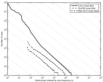
Figure 1: Data collected from shared objects on several unix platforms, showing the number of references to library subroutines. The observed number of references shows good agreement with Zipf-style frequency laws of the form $c\cdot n^{-1}$ (dotted diagonal lines). A detailed explanation of this data is given in Section 6.

It is known that hardware instruction frequencies follow an iconic curve described by George K. Zipf for word use in natural languages [16, 18, 27]. Zipf noted that if words in a natural language are ranked according to use frequency, the frequency of the $n^{\mathit{th}}$ word is about $n^{-1}$. Zipf-style empirical laws crop up in many fields [24, 21]. Evidence suggests programming language constructs also follow a Zipf-like law [5, 17]. It is natural then to wonder if this result might extend to library components. Our results support this conclusion. Figure 1 shows the reuse counts of subroutines in shared objects on three Unix platforms, clearly showing Zipf-like $n^{-1}$ curves. These results are described in detail in Section 6. The appearance of such curves is not happenstance. In Section 4.2 we argue they are a direct result of programmers trying to write as little code as possible by reusing library subroutines; this drives reuse rates toward a “maximum entropy” configuration, namely a Zipf’s law curve.

1.1 Organization

The remainder of this paper is organized as follows. Section 2 introduces an abstract model of software reuse from which we derive our results. In Section 3 we give a brief overview of Kolmogorov complexity. In Section 4 we derive bounds on the rates at which software components may be reused, and give an account for the appearance of Zipf-style empirical laws. Section 5 examines the potential for software reuse as a function of the parameter $H$. In Section 6 we present some preliminary experimental results, and Section 7 concludes.

2 Modelling library reuse

In this section we propose an abstract model capturing some essential aspects of software reuse within a problem domain. The basic scenario is this: we have a library, possibly many libraries that we collectively consider as one, that contains a great number of software components. These components may be subroutines, architectural skeletons, design patterns, generics, component generators, or whatever form of abstraction we may yet invent; their precise nature is unimportant for the argument. In using a component from the library we achieve some reduction in the size of the program, and perhaps consequently, in the effort required to implement it. Program size serves as a rough lower bound to effort, but it would be a grave error to confuse the two.

2.1 Distribution of programs in a domain

We presume that the projects undertaken by programmers working in a problem domain can be modelled by a probability distribution on programs. The probability distribution is defined on “uncompressed” programs that do not use any library components. These uncompressed programs can be viewed as specifications that programmers set out to realize.

We consider compiled programs modelled by binary strings on the alphabet $\{0,1\}$. We write $\|w\|$ for the length of a string $w$. Finite programs are countably infinite in number, so we immediately encounter the problem of defining a probability distribution in which the probability of encountering individual programs may be infinitesimal. A rigorous approach would be to employ measure theory, for example Loeb measure, which would allow us to speak of the probability of individual programs. This would require some rather daunting machinery and we instead settle for a more accessible approach similar to that used by [4, 6, 25].

Let $A^{\leq n}=\{w\in\{0,1\}^{\ast}~{}:~{}\|w\|\leq n\}$ denote compiled programs of length at most $n$ bits. We introduce a family of conditional distributions $\{p_{s_{0}}\}_{s_{0}\in\N}$ whose domains consist of programs $\leq s_{0}$ bits in size, that is,

$$p_{s_{0}}:A^{\leq s_{0}}\rightarrow\R$$

and satisfying $\sum p_{s_{0}}=1$ and $p_{s_{0}}(w)\geq 0$. The intent is that $p_{s_{0}}(w)$ gives the probability that someone working in the problem domain will set out to realize the particular (uncompressed) program $w$, given that $w$ is at most $s_{0}$ bits long. For this family of distributions to be compatible with one another we require that $p_{s_{0}}(w)=p_{s_{0}+1}(w~{}|~{}\|w\|\leq s_{0})$, i.e., we can get the distribution on length $\leq s_{0}$ programs by taking a conditional probability on the distribution for length $s_{0}+1$ programs. We do not presume that such distributions can be effectively described.

In what follows we use the usual notation for expectation with the implied assumption of $s_{0}\rightarrow\infty$; for example, if $f:\{0,1\}^{\ast}\rightarrow\R$ maps programs to real numbers, then by $E[f(w)]$ we mean:

$$E\bigl{[}f(w)\bigr{]} \equiv\lim_{s_{0}\rightarrow\infty}\sum_{w:\|w\|\leq s_{0}}f(w)p_{s_{0}}(w)$$

if such a limit should exist. For example, a mean program size $E\bigl{[}\|w\|\bigr{]}$ may exist for a problem domain, but we do not require nor expect this.

2.2 The entropy parameter $H$

A key, perhaps defining, feature of a problem domain is that there is similarity of purpose in the programs people write. We do not expect the distribution of programs written in a problem domain to be uniform over all possible programs, but rather concentrated on programs that solve certain classes of problems typical for the domain. We formalize this intuition by introducing a parameter $H$ for problem domains measuring how far their probability distribution departs from uniform. This $H$ is very similar to entropy rate from information theory, and coincides if we are willing to assume programs are drawn from a stationary stochastic process. When $H=1$ the distribution over programs is uniform, modelling extreme diversity of software, with little opportunity for reuse. For $H<1$ there is some potential for reuse. In fact as we shall see shortly, we may expect that up to a proportion $1-H$ of programs may be reused from libraries.

Define the entropy of each distribution $p_{s_{0}}$ in the standard way (see, e.g., [7, 19]):

$$H(p_{s_{0}}) =\sum_{w:\|w\|\leq s_{0}}-p_{s_{0}}(w)\log_{2}p_{s_{0}}(w)$$

This is the expected number of bits required to represent a program of size $\leq s_{0}$ in this domain. We are interested in the limit behaviour of $\frac{1}{|A^{\leq s_{0}}|}H(p_{s_{0}})$, akin to the entropy rate of a random process. In general this limit may not exist — there might be oscillations — so we need some weaker notion of limit. We settle for a limsup, which gives an almost sure upper bound on the limit behaviour.

Definition 1 (Entropy parameter).

Define the entropy parameter $H$ of a problem domain to be the greatest value that $\frac{1}{|A^{\leq s_{0}}|}H(p_{s_{0}})$ attains infinitely often as $s_{0}\rightarrow\infty$:

$$H =\limsup_{s_{0}\rightarrow\infty}\left(\frac{1}{|A^{\leq s_{0}}|}H(p_{s_{0}})\right)$$

As a consequence of this definition we are guaranteed that $H(p_{s_{0}})\leq s_{0}H$ almost surely as $s_{0}\rightarrow\infty$.

We cannot hope to calculate $H$ from first principles except for toy scenarios, but there is hope we might estimate it empirically. We introduce $H$ primarily as a theoretical tool to model problem domains in which people have great similarity of purpose ($H\rightarrow 0$) or diffuse interests ($H\rightarrow 1$). The main impact of $H$ is the following.

Figure 2: The basic scenario: programmers in a problem domain set out to realize a program that can be represented in $s$ bits when compiled without the use of a library. By using library components, they are able to reduce the size of the compiled program, down to an expected size of $\geq Hs$ bits.

Claim 2.1.

In a problem domain with entropy parameter $H$, the expected proportion of code that may be reused from a library is at most $1-H$.

This is a consequence of the Noiseless Coding Theorem of information theory (e.g., [1, §2.5]), which states that coding random data with entropy $H$ requires (on average) at least $H$ bits. Suppose an uncompressed program has size $s\leq s_{0}$. We defined $H$ so that $H(p_{s_{0}})\leq sH$ almost surely, so we can compress programs to an expected size of at best $sH$ by the Noiseless Coding Theorem. Therefore the expected amount of code saved by use of the library is at most $(1-H)s$, and it is reasonable to equate this with the amount of code reused from the library. An immediate implication is that blanket reuse prescriptions such as “effective organizations reuse 70% of their code from libraries” are unrealistic; reuse goals need to be pegged to the problem domain’s value of $H$.

Figure 2 illustrates the scenario we consider in this paper: programmers set out to implement the capabilities of some uncompressed program of length $s$ written without use of a library, drawn from the distribution for the problem domain. A programmer implements the program making use of the library, effectively “compressing” it. The expected size of the compressed program is at least $Hs$ bits, by the previous arguments. The library consists of a set of components, each with an identifier or codeword by which they are referred to. We always take programs to be compiled, so as not to care about the high compressibility of source representations.

2.2.1 Motifs and the AEP

One question we should like to answer is whether when $H<1$ there are commonly occurring patterns or “motifs” in programs that we can put in libraries and reuse to compress programs. If we are willing to assume that programs in a problem domain behave as if excerpted from a stationary ergodic source, then the Shannon-McMillan-Breiman theorem (asymptotic equipartition property or AEP) [7, §15.7] ensures that when $H<1$ there are commonly occurring finite subsequences in programs that can be exploited, and indeed that we can achieve optimal compression of programs merely by having libraries of common instruction sequences. That more complex software components prove necessary in practice suggests the stationary ergodic assumption is too strong, and a weaker ergodic property is needed to account for the emergence of motifs in software when $H<1$. It is unclear yet exactly what this property might be; in the remainder of this paper we do not assume AEP.

2.3 Libraries maximize entropy

A truly great computer programmer is lazy, impatient and full of hubris. Laziness drives one to work very hard to avoid future work for a future self. — Larry Wall

Programmers, so we read, are lazy— they write libraries to capture commonly occurring abstractions so they do not have to write them over and over again. The social processes that drive programmers to develop libraries have an interesting theoretical effect. We can view programmers contributing to domain-specific libraries as collectively defining a system for compressing programs in that domain. If there is a common pattern, eventually someone will identify it and put it in a library. Since the absence of common patterns in code is implied by high entropy, we propose the following principle.

Principle 1 (Entropy maximization).

Programmers develop domain-specific libraries that minimize the amount of frequently rewritten code for the problem domain. This tends to maximize the entropy of compiled programs that use libraries.

As evidence for this principle, we show in Section 6 that the rate at which library components are reused is empirically observed to approach a maximum entropy configuration.

In practice programmers have to strike a balance between the succinctness of their programs and their readability; see, e.g., [11] for an elegant discussion of such tradeoffs. However, we maintain that the drive toward terseness and factoring common patterns is a defining pressure on library development: entropy is essentially a measure of communication efficiency, and programmers edge as close to maximum entropy as they can while maintaining source-code understandability.

2.4 The Platonic library

In the early days of computing libraries held a hundred subroutines at most; these days it is common for computers to have a hundred thousand subroutines available for reuse (cf. Section 6). Let us suppose that as time goes on we shall continue to add components to our libraries as we discover useful abstractions and algorithms. Our current libraries might be viewed as a truncated version of some infinite (but countable) library toward which we are slowly converging. It is convenient to pretend that this limit already exists as some infinite “Platonic library” for the problem domain, and that we are merely discovering ever-larger fragments of it, recalling Erdös’ book of divine mathematical proofs. Were we granted access to the entire library, we might write software in a very efficient way. We use the Platonic library as a device — a convenient fiction — to reason about how useful finite libraries might be.

Infinite objects need to be treated with care. We shall not assume that some “optimal infinite library” exists that is the best possible such library. Nor shall we assume there is some finite description or computable enumeration of its contents. We merely assume that fragments of the Platonic library give us snapshots of what shall be in our software libraries over time.

2.5 Existence of reuse rates

Numerous metrics have been proposed for measuring reuse. We focus on the reuse rate of a component, which we write $\lambda(n)$ and define as the expected rate at which references are made to the $n^{\mathit{th}}$ library component in a compressed program. The units of $\lambda(n)$ are expected references per bit of compiled code. We assume mean reuse rates exist in a problem domain, in the following sense.

Assumption 1.

Let $\mathrm{Refs}_{n}(w)$ count the number of references to the $n^{\mathit{th}}$ component in a compressed program $w$ of size $\leq s_{0}$. We assume that

$$E\Bigl{[}\mathrm{Refs}_{n}(w)~{}\Bigm{|}~{}\|w\|=s\Bigr{]}~{}~{}\sim~{}~{}\lambda(n)s+o(s)~{}~{}~{}~{}\mathrm{as}~{}s_{0}\rightarrow\infty$$ (1)

where $o(s)$ denotes some error term growing asymptotically slower than $s$.

We unfortunately do not have a good sense of how to go from the problem domain’s distributions $p_{s_{0}}$ on uncompressed programs to rates of components in compressed programs; this is tied up with the ergodic process issues mentioned in Section 2.2. We dodge the issue by simply assuming that the mean rates $\lambda(n)$ exist. This is not a demanding assumption; many sensible random process models would imply Assumption 1, for example modelling component uses as a renewal process (see, e.g., [26, §3]).

2.6 Ordering of library components

For convenience we shall suppose the library components are arranged in decreasing order of expected reuse rate in the problem domain: that is,

$$\lambda(n)\geq\lambda(n+1)$$

There are two reasons for this. The first is tidiness, so that when we plot $\lambda(n)$ vs $n$ we see a monotone function and not noise. The asymptotic bounds we derive on $\lambda(n)$ do not rely on this ordering. The second reason is that to derive bounds on how well we might compress programs we need to assign shorter identifiers to more frequently used components. This is easiest to reason about if the Platonic library is sorted by use frequency.

3 Kolmogorov Complexity

Kolmogorov complexity, also known as Algorithmic Information Theory, was founded in the 1960s by R. Solomonoff, G. Chaitin, and A.N. Kolmogorov. We shall only make use of some basic facts; for a more thorough introduction the survey article [20] or the book [19] are recommended. The central idea is simple: measure the ‘complexity’ of an object by the length of the smallest program that generates it. This generalizes to the study of description systems, that is, systems by which we define or describe objects, of which programming languages, logics, and descriptive set theory are prominent examples. The source code of a program, for example, describes a program behaviour; a set of axioms describes a class of mathematical structures. In the general case we have some objects we wish to describe, and a description system $\phi$ that maps from a description $w$ (for us, a program) to objects. The usual situation is to describe an object by exhibiting a program that generates it; in this case we may also provide some inputs to the program, which we shall call parameters. The Kolmogorov complexity of an object $x$ in the description system $\phi$, relative to a parameter $y$ is defined by:

$$C_{\phi}(x~{}|~{}y)=\min_{w}\{\|w\|:\phi_{w}(y)=x\}$$ (2)

In the case where the description system $\phi$ is a programming language, we may read Eqn. (2) as finding the shortest program that, given input parameter $y$, outputs $x$. The parameter $y$ does not contribute to the measured description length $C_{\phi}(x~{}|~{}y)$. Without a parameter we have the simpler case $C_{\phi}(x)=C_{\phi}(x~{}|~{}\epsilon)$ where $\epsilon$ is the empty string.

For example, we might choose the programming language Java as our description system; then for some string $x$, its Kolmogorov complexity $C_{\mathsf{Java}}(x)$ is the length of the shortest program that outputs $x$. To determine whether use of a library $\mathsf{L}$ offers a reduction in program size, we can consider the combination of Java and the library $\mathsf{L}$ as a description system itself which we might call $\mathsf{Java}+\mathsf{L}$, and compare $C_{\mathsf{Java+L}}(x)$ to $C_{\mathsf{Java}}(x)$.

A very useful insight is that the choice of language doesn’t much matter.

Fact 3.1 (Invariance [19, §2.1]).

There exists a universal machine $U$ such that if $\phi$ is some effective description system (e.g., a programming language) then there is a constant $c$ such that $C_{U}(x)\leq C_{\phi}(x)+c$ for any $x$.

That is, the universal machine $U$ is optimal up to a constant factor. For this reason the subscript $U$ can be dropped and one can write $C(x)$ for the Kolmogorov complexity of $x$, knowing it is only defined up to some constant factor.

Some strings have very short descriptions: a string of a trillion zeros may be produced by a short program. Others require descriptions as long as the strings themselves, for instance a million digit binary string obtained from a physical random bit generation device. A recurrent theme in Kolmogorov complexity is that there are never enough descriptions to go around so as to give short descriptions to most objects. In the case where both the objects and their descriptions are binary strings, we have the following well-known result that the probability we can save more than a constant number of bits in compressing randomly selected strings is zero.

Fact 3.2 (Incompressibility [19, §2.2]).

Suppose $g:\N\rightarrow\N$ is an integer function with $g(n)>0$ and $g\in\omega(1)$, that is, $\lim_{n\rightarrow\infty}g(n)=\infty$. Let $x$ be a string chosen uniformly at random. Then almost surely:

$$C_{\phi}(x)\geq\|x\|-g\bigl{(}\|x\|\bigr{)}$$ (3)

Fact 3.2 implies, for example, that one cannot devise a coding system that compresses strings by even $\log\log n$ or $\alpha^{-1}(n,n)$ (inverse Ackermann) bits with nonzero probability. The proof of Fact 3.2 uses counting arguments only, with no appeal to computability of the description system. Therefore the inequality (3) applies to any description system $\phi$, even description systems that are not computable. For example, Fact 3.2 even applies if we permit ourselves to use an infinite, not computably enumerable library as we described in Section 2.4. However, it does not apply in the case where there is a nonuniform distribution, as in problem domains where $H<1$.

In the remainder of this paper we shall assume compiled programs are incompressible in the sense of Fact 3.2.

Proposition 3.1.

Compiled C programs on existing major architectures are almost surely Kolmogorov incompressible.

Note that “almost surely Kolmogorov incompressible” does not imply anything about the compressibility of typical compiled programs for a problem domain. Rather, it means that if one chooses a valid compiled program uniformly at random, with probability 1 it cannot be replaced by a shorter program with the same behaviour. In subsequent sections we investigate problem domains where there is a nonuniform distribution on programs, i.e., $H<1$, where the situation is rosier.

We sketch a proof of Proposition 3.1, showing that the number of distinct behaviours described by compiled programs of $s$ bits grows as $\sim 2^{s}$ on current machines, which implies compiled programs are almost surely (Kolmogorov) incompressible. The C language has the useful ability to incorporate chunks of binary data in a program. For example, the binary string $z=0110100111011010$ may be encoded by the C declaration

$$\mathsf{unsigned}~{}\mathsf{char}~{}\mathsf{z}[2]=\{\mathsf{0x69},\mathsf{0xda}\};$$

Moreover, such arrays are laid out as contiguous binary data in the compiled program, so that a binary string of length $m$ bytes requires exactly $m$ bytes in the compiled program. We can package such an array with a short program of constant size that reads the binary string from memory and outputs it to the console. Every binary string of $m$ bytes may be encoded by such a compiled program of size at most $c+m$ bytes, where $c$ is a constant representing the overhead of a read-print loop. Every such program yields a unique behaviour, so the number of distinct behaviours of compiled programs of $s$ bits is $\sim 2^{s}$. We can then adapt the argument used to prove Fact 3.2, replacing strings by compiled programs, which shows compiled C programs are almost surely incompressible.

Note that uncompiled programs are highly compressible. For example, C language source code may not contain certain bytes (e.g., control characters) such as the null character $0x00$. This means they can be compressed by a factor of (at least) $\frac{1}{256}\sim 0.39\%$. Restricting our attention to compiled programs is crucial.

4 A bound on reuse rates

In this section we derive a bound on the reuse rate $\lambda(n)$ at which the $n^{\mathit{th}}$ library component is reused in ‘compressed’ programs written with use of a library.

4.1 Coding of references

We need some rudimentary accounting of what we gain and lose by use of the library: we save some by using a library component, at the cost of having to refer to it. Let us first consider the cost of referring to components.

We presume that unique identifiers are assigned to library components; we call these codewords. Let $c(n)$ be the binary codeword for the $n^{\mathit{th}}$ library component, and $\|c(n)\|$ its length. Optimal strategies such as Shannon-Fano or Huffman codes assign shortest codewords to the most frequently needed components. Since our library is sorted in order of use frequency (Section 2.6), we may presume that $\|c(n)\|\leq\|c(n+1)\|$, i.e., codeword lengths are nondecreasing as we go down the list of components.

In what follows we want to make asymptotic arguments, and fixing an identifier size (e.g., 64 bits) would lead to wildly wrong conclusions. Instead we require that the identifier size grows with the number of components, albeit slowly. That $\|c(n)\|\geq\log_{2}n$ follows from the pigeonhole principle. Having identifiers of length only $\log_{2}n$ leads to difficulties, because they are not uniquely decodable. That is, if I am presented with a string of such identifiers I have no way to tell where one identifier stops and the next starts. (This does not arise in current architectures because of fixed word size, but as we said, care is needed in asymptotic arguments). A more accurate requirement is the following, which draws on Kraft’s inequality that uniquely decodable codes must satisfy $\sum_{n=1}^{\infty}2^{-\|c(n)\|}\leq 1$.

Proposition 4.1.

For identifiers to be uniquely decodable,

$$\|c(n)\|\geq\log^{+}n$$

where $\log^{+}n=\log n+\log\log n+\log\log\log n+\cdots$ and the sum is taken only over the positive real terms.

We omit the proof; see e.g., [25, §2.2.4] or [19, §1.11.2] (in particular problem 1.11.13).

4.2 Derivation of reuse rate bound

We now derive an asymptotic upper bound on the rates $\lambda(n)$ at which library components may be reused. We do this under the assumption that each time a library component is used in a program, the same identifier is used to refer to it, i.e., there is no recoding of identifiers. Our argument follows standard lines [24] but adapted to coding of library references under the model laid out in Section 2.

Theorem 4.1.

Without recoding of identifiers, the asymptotic reuse rates $\lambda(n)$ must satisfy $\lambda(n)\prec(n\log n\log^{+}n)^{-1}$.

Proof.

We count the size of the references to library components within compressed programs (i.e., those written with use of a library). Consider programs of length at most $s$. As $s\rightarrow\infty$, the expected number of occurrences of the $n^{\mathit{th}}$ component tends to $\lambda(n)s+o(s)$ under Assumption 1. Referring to the $n^{\mathit{th}}$ component requires at least $\log^{+}n$ bits (Proposition 4.1). We need only consider components whose identifier length is less than $s$, since identifiers longer than the program would not fit. Therefore we consider only up to component number $2^{s}$ since $\log^{+}2^{s}\geq s$.

The expected total size of all the references to components is then at least:

$$\sum_{n=1}^{2^{s}}\underbrace{\bigl{(}\lambda(n)s+o(s)\bigr{)}}_{\text{\# refs}}\underbrace{\log^{+}n}_{\text{ref size}}$$

The references to components are contained within the program, and therefore their total size must be less than $s$, the size of the program. Therefore we have an inequality:

$$\sum_{n=1}^{2^{s}}\bigl{(}\lambda(n)s+o(s)\bigr{)}\log^{+}n \leq s$$ (4)

Dividing through by $s$ and taking the limit as $s\rightarrow\infty$,

$$\lim_{s\rightarrow\infty}\sum_{n=1}^{2^{s}}\frac{1}{s}\bigl{(}\lambda(n)s+o(s)\bigr{)}\log^{+}n\leq 1$$ (5)

Since $\lim_{s\rightarrow\infty}\frac{1}{s}o(s)=0$ by definition,

$$\sum_{n=1}^{\infty}\lambda(n)\log^{+}n\leq 1$$ (6)

We now consider conditions under which this sum converges. (Section A.1 summarizes the asymptotic notations used here.) We argue using Proposition A.1, using a diverging series to bound the terms of Eqn. (6). The simple argument is to note that the harmonic series diverges, and therefore the terms of Eqn. (6) must grow slower than this, so $\lambda(n)\log^{+}n\prec\frac{1}{n}$, or $\lambda(n)\prec\frac{1}{n\log^{+}n}$. However, this bound is quite loose. A more slowly diverging series is $\sum_{n}\frac{1}{n\log n}$. Using this,

$$\lambda(n)\log^{+}n \prec\frac{1}{n\log n}$$

or,

$$\boxed{\lambda(n)\prec\frac{1}{n\log n\log^{+}n}}$$ (7)

This completes the proof. ∎∎

The bound of Theorem 4.1 is not tight. No tightest bound is possible using this line of argument since there is no slowest diverging sequence with which to bound a convergent sequence, a classical result due to Niels Abel. However, the bound is tight to within a factor $n^{\epsilon}$ for any $\epsilon>0$.

Entropy maximization and Zipf’s Law. Theorem 4.1 provides an upper bound on $\lambda(n)$, but it could well be the case that $\lambda(n)\sim\frac{1}{n^{3}}$, for example. Why do the curves we see in practice (e.g., Figure 1) hug the bound of Theorem 4.1? We believe the answer to why we observe $\lambda(n)\approx\frac{1}{n}$ is due to the tendency of libraries to evolve so that programmers can write as little code as possible, which in turn implies evolution toward maximum entropy in compiled code (Principle 1). The entropy rate of component references is maximized when $\lambda(n)\approx\frac{1}{n}$ (see, e.g., [13]).

5 Reuse potential

In the following sections we consider the possibilities of code reuse in two cases: (1) when $H=1$ and we have a uniform distribution on programs; (2) when $0<H<1$ and we have some degree of compressibility in the problem domain. The case $H=0$ is left for future work.

5.1 The uniform case: $H=1$

The uniform case of $H=1$, in which every program is equally likely to be implemented, reduces the scenario to classical Kolmogorov complexity with a uniform distribution on programs. It has some surprising properties that suggest $H=1$ to be an unlikely scenario for real problem domains.

Our first result concerns the number of library components we might expect to use in a program. Let $N(s)$ be a random variable indicating for a program of uncompressed size $s$ the number of components whose use reduces program size. Surprisingly, as program size increases the expected number of components that reduce program size is bounded above by a constant.

Theorem 5.1.

If $H=1$ there exists a constant $n_{\mathsf{crit}}$ independent of program size $s$ such that $N(s)\leq n_{\mathsf{crit}}$ almost surely.

Proof.

Suppose each component used saved at least 1 bit. If $\lim_{s\rightarrow\infty}E[N(s)]$ were unbounded, use of the library could compress random programs by an unbounded amount, contradicting incompressibility (Fact 3.2). ∎∎

This has a simple corollary concerning the potential for code reuse.

Corollary 5.1.

When $H=1$ the expected proportion of a program that can be reused from libraries tends to zero as program size increases.

Because of these results, the case $H=1$ is somewhat uninteresting and does not seem to model real life, where we know libraries are useful and let us reduce the size of programs. In the next sections we examine the more interesting case of $0<H<1$, where we can compress programs, even ones that are (Kolmogorov) incompressible, by use of a library.

5.2 The nonuniform case: $0<H<1$

More interesting than the uniform case is the situation when $0<H<1$, which implies a nonuniform distribution on programs. This models problem domains that have some potential for code reuse, and libraries are of central importance in reducing program size. Recall from Section 2.2 that we can expect to compress programs in such domains from uncompressed size $s$ to at best $Hs$ by use of a library. A standard result from information theory can be adapted to show this bound is achievable, at least in a theoretical sense.

Claim 5.1.

There exists a library with which uncompressed programs of size $s$ can be compressed to expected size $\sim Hs$.

The proof of this is not particularly illustrative and we banish it to a footnote. The gist is to place every possible program into the library as a “component,” but ordering them so that the most likely programs for the problem domain come soonest in the library order and thus are assigned the shortest codewords. This is a wildly impractical construction but demonstrates the claim. In practice we decompose software into reusable chunks that we put in libraries; that reusable chunks exist suggests an ergodic property (see Section 2.2.1).

Unlike the situation of $H=1$ where the number of components useful for a program was at most a constant, when $0<H<1$ we have a much more pleasing situation: the number of useful components increases steadily as we increase program size.

5.2.1 The incompleteness of libraries

Under reasonable assumptions we prove that no finite library can be complete: there are always more components we can add to the library that will allow us increase reuse and make programs shorter. To make this work we need to settle a subtle interplay between the Kolmogorov complexity notion of compressibility (there is a shorter program doing the same thing) and the information theoretic notion of compressibility (low entropy over an ensemble of programs). Now because we defined probability distributions on programs (rather than behaviours), we run into the possibility that the probability distribution might weight heavily programs that are Kolmogorov compressible, i.e., the distribution might prefer programs $w$ with $\|w\|>>C(w)$. For example, a problem domain might have programs that are usually compressible to half their size not because the probability distribution focuses on a particular class of problems, but because we artificially defined $p_{s_{0}}$ to select only those programs that are twice as large as they might be (for example, we might pad every likely program with many $\mathsf{nop}$ instructions.) To avoid this difficulty we require the distributions be honest in the following sense.

Definition 2 (Honesty).

We say the distributions $p_{s_{0}}$ for a problem domain are honest if the programs are Kolmogorov incompressible. Specifically,

$$E\left[\frac{C(w)}{\|w\|}\right]\rightarrow 1 ~{}~{}~{}~{}\text{as }s_{0}\rightarrow\infty$$ (8)

where the expectation is taken over the distributions $p_{s_{0}}$. This requires that the probability distribution does not artificially prefer verbose programs with $\|w\|>>C(w)$.

If the distribution for a problem domain is honest and has $H<1$, the programs are expected to be information-theoretically compressible by use of a library, but not Kolmogorov compressible. In other words, our ability to compress programs is due to a “focus” on a class of problems of interest to the domain, not just an artificial selection of overly-verbose programs.

Inspired by Euclid’s proof that there are infinitely many primes, with the honesty assumption we can prove there are infinitely many reusable software components that make programs shorter.

First we need two smaller pieces of the puzzle.

Lemma 5.1.

If $H>0$ then for any finite $k$, $Pr(\|w\|\leq k)\rightarrow 0$ as $s_{0}\rightarrow\infty$.

Proof.

We know from definition of $H$ that $H(p_{s_{0}})=Hs_{0}$ infinitely many times as $s_{0}\rightarrow\infty$ (Section 2.2). Consider how probability must be distributed among programs of different lengths to account for this much entropy. We try to account for as much entropy as we can by short programs, setting a uniform distribution $p(w)=\frac{1}{2^{Hs_{0}}}$ on the first $2^{Hs_{0}}$ programs— this is the fewest number of programs that would produce this much entropy. To programs of length $\leq k$ we can account for

$$\sum_{i=0}^{k}2^{i}\cdot\left(-\frac{1}{2^{Hs_{0}}}\log\frac{1}{2^{Hs_{0}}}\right)\sim 2^{k+1-Hs_{0}}Hs_{0}$$

bits of entropy. But as $s_{0}\rightarrow\infty$, $2^{k+1-Hs_{0}}Hs_{0}\rightarrow 0$ so we can account for none of the entropy by programs of length $\leq k$. Therefore $Pr(\|w\|\leq k)\rightarrow 0$ as $s_{0}\rightarrow\infty$. ∎

Lemma 5.2.

If $H>0$ then $E\left[\frac{1}{\|w\|}\right]\rightarrow 0$ as $s_{0}\rightarrow\infty$.

Proof.

Suppose $E\left[\frac{1}{\|w\|}\right]=c$ for some $c>0$. Then there would be a finite probability that $\|w\|\leq c^{-1}$ as $s_{0}\rightarrow\infty$, contradicting Lemma 5.1. ∎

Now we are ready for the main theorem, which proves no finite library can be “complete” in the sense of achieving a compression ratio of $H$ when $0<H<1$.

Theorem 5.2 (Library Incompleteness).

If a problem domain has $0<H<1$ and honest distributions (Defn. 2), no finite library can achieve an asymptotic compression ratio of $H$.

Proof.

Suppose a finite library of components achieves a compression factor $1-\epsilon$, with optimal compression when $1-\epsilon=H$. Call the programming language $\phi$ and the library $L$. We can write an interpreter for $\phi$ that incorporates the library $L$; since the library is finite this is a finite program. We call the resulting machine model $\phi+L$. Consider Kolmogorov complexity for this machine, writing $C_{\phi+L}(w)$ for the size of the smallest $\phi$-program using $L$ that has the same behaviour as $w$. Saying the machine $\phi+L$ achieves the compression factor $1-\epsilon$ implies

$$E\left[\frac{C_{\phi+L}(w)}{\|w\|}\right]=1-\epsilon$$ (9)

From the invariance theorem of Kolmogorov complexity (Fact 3.1) we have that there exists a constant $c$ such that

$$C(w)\leq C_{\phi+L}(w)+c$$ (10)

for every program $w$. Dividing through by $\|w\|$ and taking expectation,

$$E\left[\frac{C(w)}{\|w\|}\right]\leq\underbrace{E\left[\frac{C_{\phi+L}(w)}{\|w\|}\right]}_{=1-\epsilon}+E\left[\frac{c}{\|w\|}\right]$$ (11)

From honesty $E\left[\frac{C(w)}{\|w\|}\right]\rightarrow 1$, and from Lemma 5.2 we have $E\left[\frac{c}{\|w\|}\right]\rightarrow 0$. Therefore (11) is, in the limit as $s_{0}\rightarrow\infty$:

$$1\leq(1-\epsilon)+0$$

For this inequality to hold, $\epsilon\rightarrow 0$ for any finite library. Therefore no finite library can achieve an asymptotic compression ratio $<1$ when the distributions are honest. ∎∎

Claim 5.1 showed that an infinite library can achieve expected size $\sim Hs$; Theorem 5.2 shows that no finite library can. Therefore only infinite libraries can compress programs of size $s$ to expected size $Hs$. However, this is an asymptotic argument; if we restrict ourselves to programs of size $\leq s_{0}$ for some fixed $s_{0}$, finite libraries can approach a compression ratio of $Hs$ by including more and more components. Doug Gregor suggested calling Theorem 5.2 the Full Employment Theorem for Library Writers, after Andrew Appel’s boon to compiler writers. Theorem 5.2 has a straightforward implication: no finite library can be complete; there are always more useful components to add. In practice we have a tradeoff between the utility of larger libraries and the economic cost of producing them; this suggests the importance of designing libraries for extensibility.

A minor change to the above proof yields a similar but slightly stronger result.

Corollary 5.2.

If a problem domain has $0<H<1$ and honest distributions, no computably enumerable library can achieve a compression ratio of $H$.

Proof.

Repeat the proof of Theorem 5.2, replacing “finite library” with “c.e. library.” In particular the choice of a c.e. library guarantees that the interpreter for $\phi+L$ is a finite program: whenever a library subroutine is required, it can be generated from the program enumerating the library. ∎∎

We may casually equate “not computably enumerable” with “requires human creativity.” Corollary 5.2 indicates that the process of discovering new and useful library components is not a process that can can be fully automated.

5.2.2 Size of library components.

We now consider how big library components might be. If we want to achieve the strong reuse vision of “programming by wiring together large components,” this suggests that components ought to be quite large compared to the wiring. The following theorem sheds light on the conditions when this is possible.

Let $S(n)$ denote the expected amount of code (in bits) saved per use of the $n^{\mathit{th}}$ component. We consider the case when $\lambda(n)\sim\frac{1}{n\|c(n)\|f(n)}$, where $\|c(n)\|$ is the codeword (identifier) length, and $f(n)$ is a function $f\in o(n^{\epsilon})$ for $\epsilon>0$ that ensures convergence (cf. Section 4.2). This coincides with a Zipf-style law as observed in practice (Figure 1).

Theorem 5.3.

If a library achieves a compression factor of $H>0$ in an honest problem domain, then $S(n)\sim\frac{1-H}{H}\cdot o(n^{\epsilon})$ for any $\epsilon>0$.

Proof.

Summing over all components, the total code saved is:

$$\sum_{n=1}^{\infty}\underbrace{\bigl{(}\lambda(n)Hs+o(Hs)\bigr{)}}_{\text{expected \# uses}}~{}~{}\cdot\underbrace{S(n)}_{\text{savings per use}}=\underbrace{(1-H)s}_{\text{total savings}}$$ (12)

Dividing through by $Hs$ and taking the limit as $s\rightarrow\infty$, and substituting $\lambda(n)\sim\frac{1}{n\|c(n)\|f(n)}$,

$$\sum_{n=1}^{\infty}\frac{1}{n\|c(n)\|f(n)}S(n)=\frac{1-H}{H}$$

Now if $S(n)\sim n^{a}$ for some constant $a>0$ then the sum would diverge. Therefore $S(n)$ is not polynomial in $n$; in fact for the sum to converge we must have $S(n)\prec f(n)$ which means $S(n)$ behaves asymptotically as

$$S(n)\sim\frac{1-H}{H}o(n^{\epsilon})$$

where $o(n^{\epsilon})$ denotes some subpolynomial function. ∎∎

Note that if the components in the library are unique, then $S(n)\geq\log n$ by pigeonhole.

Figure 3: Plot of $\frac{1-H}{H}$ versus $H$, indicating how much code is saved, proportionately, per component use. When $H\rightarrow 1$ there is almost no reuse; $H\rightarrow 0$ coincides with the “strong reuse” ideal of wiring together large components. In between is weak reuse, with moderate amounts of code drawn from libraries.

Strong reuse? The interpretation of Theorem 5.3 is fairly intuitive. Roughly it says the savings we can expect per component are linear in the size of the component identifier. Which is to say, we should expect savings for the $n^{\mathit{th}}$ component to grow roughly as $\log^{+}n$. This is consistent with findings in the reuse literature that small components are much more likely to be reused. The important factor here is the multiplier $\frac{1-H}{H}$. As $H\rightarrow 0$, this multiplier becomes arbitrarily large. This suggests that “strong reuse” (Section 1) corresponds to the region $H\rightarrow 0$. For example, if programs in a problem domain are thought to be solvable by wiring together components that are (say) $1000$ times bigger than the wiring itself, this suggests $\frac{1-H}{H}\approx 10^{5}$ or $H\approx 0.001$. The key result is that whether one is able to achieve strong reuse depends critically on the parameter $H$ — which measures how much diversity there is in the problem domain.

6 Experimental data collection

Preliminary empirical data was collected from three large Unix installations. The problem domain is not particularly well-defined, but is rather “the mishmash of things one wants to do on a typical research Unix machine.” On the SunOS and Mac OS X machines we located every shared object and used the unix commands $\mathsf{nm}$ or $\mathsf{objdump}$ to obtain a listing of the relocatable symbols (i.e., references to subroutines in shared libraries). For the Linux machine, a more sophisticated approach was used that involved disassembling every executable object and decoding the PLT and GOT tables for shared library calls. For this reason the Linux data is much more fine-grained and reliable; for example, our data set for Linux includes the frequencies of all the x86 machine instructions, in addition to almost a half-million subroutines.

Operating System	# Objects	# Components
Linux (SuSE)	12136	455716
SunOS	23774	110306
Mac OS X	2334	37677

We counted the number of references to each component, sorted these by frequency, and this data is plotted in Figure 1. The observed counts match nicely the asymptotic prediction made in Section 4.2 (the family of curves $cn^{-1}$ is shown as dotted lines). To account for machine instructions, which are not included in the tally for the Mac OS X and SunOS machines but constitute by far the most frequently occurring software components, we started numbering the components for these machines at $n=50$. Without this adjustment the rates have a characteristic “flat top” and then rapidly converge to $n^{-1}$ lines; this is an artifact of the log-log scale.

The pronounced “steps” in the data for large $n$ occur because there are many rarely-used subroutines with only a few references; this is typical of such plots (see, e.g., [24]).

Another prediction that may follow from our model is that the number of distinct components used in a program should approach a normal distribution: under maximum entropy conditions the use of components is statistically independent, and so the central limit theorem applies. This is reminiscent of the Erdös-Kac theorem [8] that the number of prime factors of integers converges to a normal distribution. Figure 4 shows some preliminary results that support this result, drawn from the SuSE Linux data. The number of component references have been normalized by an estimated variance of $\sigma^{2}=cs^{2}$ where $s$ is the program size. Subfigure (c) shows a suggestively shaped distribution for the inset box of (a), a region where there is good “saturation” of the problem domain with programs.

Our preliminary data demonstrates a Heaps’ style law for vocabulary growth [14, §7.5]: the number of unique components encountered in examining the first $s$ bytes of the corpus grows roughly as a power law $s^{\alpha}$ with $\alpha\approx 0.8$. We have not found a satisfactory theoretical explanation.

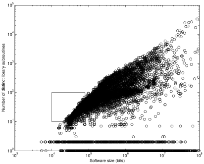
(a) Scatter-plot of the number of subroutine references

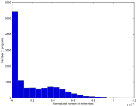
(b) Distribution histogram

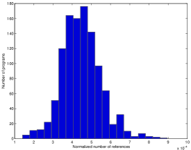
(c) Distribution for inset box

Figure 4: Data suggesting a library analogue of the Erdös-Kac theorem. (a) A scatter-plot showing the number of distinct library subroutines used vs. software size for the Linux RPM data. (b) Histogram for the number of references, normalized (see text). (c) Histogram only for the inset box of (a), illustrating an Erdös-Kac-style normal distribution for the number of components used in software. Such plots might provide a useful tool for assessing the extent of reuse vs. ideal predictions from a model.

7 Conclusion

We have developed a theoretical model of reuse libraries that provides good agreement, we feel, with our intuitions, the literature, and the preliminary experimental data we have collected on reuse on Unix machines. Much of what we have done has served to emphasize the importance of this one quantity, $H$, the entropy rate we associate with a problem domain. It determines if we can have strong reuse ($H\rightarrow 0$), or whether we can have weak reuse $(0<H<1)$, and how much code we might be able to reuse from libraries: at most $1-H$.

We have shown that libraries allow us to “compress the incompressible,” reducing the size of programs that are Kolmogorov-incompressible by taking advantage of the commonality exhibited by programs within a problem domain. We have also shown that libraries are essentially incomplete, and there will always be room for more useful components in any problem domain.

The arguments made here are quite general and might adapt easily to other description systems, for example, the reuse of abstractions, lemmas and theorems in mathematical proofs.

8 Acknowledgments

This paper benefited immeasurably from discussions with my colleagues at Indiana University Bloomington. In particular I thank Andrew Lumsdaine, Chris Mueller, Jeremy Siek, Jeremiah Willcock, Douglas Gregor, Matthew Liggett, Kyle Ross, and Brian Barrett for their valuable suggestions. I thank Harald Hammerström for letting me disappear with his copy of Li and Vit nyi [19] for most of a year.

Appendix A Background

A.1 Asymptotics

Here we recall briefly some facts and notations concerning asymptotic behaviour of functions and series. For a more detailed exposition we suggest [10].

Asymptotic notations. For positive functions $f(n)$ and $g(n)$, we make use of these notations for asymptotic behaviour:

$$f(n)\sim g(n)~{}~{} \Longleftrightarrow~{}~{}\lim_{n\rightarrow\infty}\frac{f(n)}{g(n)}=1$$ (13)

$$f(n)\prec g(n)~{}~{} \Longleftrightarrow~{}~{}\lim_{n\rightarrow\infty}\frac{f(n)}{g(n)}=0$$ (14)

$$f(n)\preceq g(n)~{}~{} \Longleftrightarrow~{}~{}\exists c\in\R~{}.~{}\lim_{n\rightarrow\infty}\frac{f(n)}{g(n)}=c$$ (15)

The “big-O” style of notation $f\in o(g)$ is equivalent to $f(n)\prec g(n)$. When we write $h(n)\sim g(n)+o(n^{2})$ we mean there exists some function $f\in o(n^{2})$ such that $h(n)\sim g(n)+f(n)$.

Series and their convergence. A series $\sum_{i=1}^{\infty}a_{i}$ is convergent when $\lim_{N\rightarrow\infty}\sum_{i=1}^{N}a_{i}$ exists in the standard reals; otherwise it is divergent. The Harmonic series $h_{n}=\frac{1}{n}$ is divergent, since $\sum_{i=0}^{\infty}h_{i}=1+\frac{1}{2}+\frac{1}{3}+\cdots$ fails to converge.

We shall make use of the following key fact for bounding convergent sequences.

Fact A.1.

Let $a_{n},b_{n}$ be positive sequences. If $\sum_{n=1}^{\infty}a_{n}$ converges and $\sum_{n=1}^{\infty}b_{n}$ diverges, then $a_{n}\prec b_{n}$.

Proposition A.1 is useful to establish a bound on the asymptotic growth of a sequence: for example, if $\sum_{n=1}^{\infty}a_{n}$ must converge, then $a_{n}\prec\frac{1}{n}$ since the harmonic series diverges.

References

- [1] Robert Ash. Information Theory. John Wiley & Sons, New York, 3 edition, 1967.
- [2] Mark Balaguer. Platonism in Metaphysics. In Edward N. Zalta, editor, The Stanford Encyclopedia of Philosophy. Summer 2004.
- [3] Victor R. Basili, Lionel C. Briand, and Walc lio L. Melo. How reuse influences productivity in object-oriented systems. Commun. ACM, 39(10):104–116, 1996.
- [4] S. Ben-David, B. Chor, O. Goldreich, and M. Luby. On the theory of average case complexity. Journal of Computer and System Sciences, 44(2):193–219, April 1992.
- [5] Daniel M. Berry. A new methodology for generating test cases for a programming language compiler. SIGPLAN Not., 18(2):46–56, 1983.
- [6] Kevin J. Compton. 0–1 laws in logic and combinatorics. In I. Rival, editor, Proceedings NATO Advanced Study Institute on Algorithms and Order, pages 353–383, Dordrecht, 1988. Reidel.
- [7] Thomas M. Cover and Joy A. Thomas. Elements of information theory. Wiley series in telecommunications. John Wiley & Sons, 1991.
- [8] P. Erdös and M. Kac. The Gaussian law of errors in the theory of additive number theoretic functions. Amer. J. Math., 62:738–742, 1940.
- [9] William B. Frakes and Christopher J. Fox. Quality improvement using a software reuse failure modes model. IEEE Transactions on Software Engineering, 22(4):274–279, April 1996.
- [10] Ronald L. Graham, Donald E. Knuth, and Oren Patashnik. Concrete Mathematics: A Foundation for Computer Science. Addison-Wesley, Reading, MA, USA, second edition, 1994.
- [11] T. R. G. Green. Cognitive dimensions of notations. In Proceedings of the HCI’89 Conference on People and Computers V, Cognitive Ergonomics, pages 443–460, 1989.
- [12] M. L. Griss. Software reuse: From library to factory. IBM Systems Journal, 32(4):548–566, 1993.
- [13] P. Harremöes and F. Topsøe. Maximum entropy fundamentals. Entropy, 3(3):191–226, 2001.
- [14] H. S. Heaps. Information retrieval: theoretical and computational aspects. Academic Press, New York, NY, 1978.
- [15] Charles W. Krueger. Software reuse. ACM Comput. Surv., 24(2):131–183, 1992.
- [16] D. Kuck. The Structure of Computers and Computations, Volume 1. John Wiley and Sons, New York, NY, 1978.
- [17] A. Laemmel and M. Shooman. Statistical (natural) language theory and computer program complexity. Technical Report POLY/EE/E0-76-020, Dept of Electrical Engineering and Electrophysics, Polytechnic Institute of New York, Brooklyn, August 15 1977.
- [18] Mario Latendresse and Marc Feeley. Generation of fast interpreters for Huffman compressed bytecode. In IVME ’03: Proceedings of the 2003 workshop on Interpreters, virtual machines and emulators, pages 32–40, New York, NY, USA, 2003. ACM Press.
- [19] M. Li and P. Vit nyi. An introduction to Kolmogorov complexity and its applications. Springer-Verlag, New York, 2nd edition, 1997.
- [20] M. Li and P. M. B. Vit nyi. Kolmogorov complexity and its applications. In Jan van Leeuwen, editor, Handbook of Theoretical Computer Science, volume A: Algorithms and Complexity. Elsevier, New York, NY, USA, 1990.
- [21] Wentian Li. Bibliography on Zipf’s Law, 2005. http://www.nslij-genetics.org/wli/zipf/index.html.
- [22] Parastoo Mohagheghi, Reidar Conradi, Ole M. Killi, and Henrik Schwarz. An empirical study of software reuse vs. defect-density and stability. In ICSE ’04: Proceedings of the 26th International Conference on Software Engineering, pages 282–292, Washington, DC, USA, 2004. IEEE Computer Society.
- [23] Jeffrey S. Poulin. Measuring Software Reuse: Princples, Practices, and Economic Models. Addison-Wesley, 1997.
- [24] David M. W. Powers. Applications and explanations of Zipf’s law. In Jill Burstein and Claudia Leacock, editors, Proceedings of the Joint Conference on New Methods in Language Processing and Computational Language Learning, pages 151–160. Association for Computational Linguistics, Somerset, New Jersey, 1998.
- [25] Jorma Rissanen. Stochastic Complexity in Statistical Inquiry, volume 15 of Series in Computer Science. World Scientific, 1989.
- [26] Sheldon M. Ross. Stochastic Processes. John Wiley and Sons; New York, NY, 2nd edition, 1996.
- [27] David Barkley Wortman. A study of language directed computer design. PhD thesis, Stanford University, 1973.