Capacity Gain from Transmitter and
Receiver Cooperation

Abstract

Capacity gain from transmitter and receiver cooperation are compared in a relay network where the cooperating nodes are close together. When all nodes have equal average transmit power along with full channel state information (CSI), it is proved that transmitter cooperation outperforms receiver cooperation, whereas the opposite is true when power is optimally allocated among the nodes but only receiver phase CSI is available. In addition, when the nodes have equal average power with receiver phase CSI only, cooperation is shown to offer no capacity improvement over a non-cooperative scheme with the same average network power. When the system is under optimal power allocation with full CSI, the decode-and-forward transmitter cooperation rate is close to its cut-set capacity upper bound, and outperforms compress-and-forward receiver cooperation. Moreover, it is shown that full CSI is essential in transmitter cooperation, while optimal power allocation is essential in receiver cooperation.

I Introduction

In ad-hoc wireless networks, cooperation among nodes can be exploited to improve system performance, and the benefits of transmitter and receiver cooperation have been recently investigated by several authors. The idea of cooperative diversity was pioneered in [1, 2], where the transmitters cooperate by repeating detected symbols of other transmitters. In [3] the transmitters forward parity bits of the detected symbols, instead of the entire message, to achieve cooperation diversity. Cooperative diversity and outage behavior was studied in [4]. Multiple-antenna systems and cooperative ad-hoc networks were compared in [5, 6]. Information-theoretic achievable rate regions and bounds were derived in [7, 8, 9, 10, 11] for channels with transmitter and/or receiver cooperation. In [12] cooperative strategies for relay networks were presented.

In this paper, we consider the case in which a relay can be deployed either near the transmitter, or near the receiver. Hence unlike previous works where the channel was assumed given, we treat the placement of the relay, and thus the resulting channel, as a design parameter. Capacity improvement from cooperation is considered under system models of full or partial channel state information (CSI), with optimal or equal power allocation.

II System Model

Consider a discrete-time additive white Gaussian noise (AWGN) wireless channel. To exploit cooperation, a relay can be deployed either close to the transmitter to form a transmitter cluster, or close to the receiver to form a receiver cluster, as illustrated in Fig. 1. In the transmitter cluster configuration, suppose the channel magnitude between the cluster and the receiver is normalized to unity, while within the cluster it is denoted by $\sqrt{g}$. The transmitter cooperation relay network in Fig. 1(a) is then described by

$$y_{1} =\sqrt{g}e^{j\theta_{2}}x+n_{1}, y =e^{j\theta_{1}}x+e^{j\theta_{3}}x_{1}+n,$$ (1)

where $x,y,n,x_{1},y_{1},n_{1}\in\mathbb{C}$, $g\geq 0$, and $\theta_{1},\theta_{2},\theta_{3}\in[0,2\pi]$: $x$ is the signal sent by the transmitter, $y$ is the signal received by the receiver, $y_{1},x_{1}$ are the received and transmitted signals of the relay, respectively, and $n,n_{1}$ are independent zero-mean unit-variance complex Gaussian random variables. Similarly, the receiver cooperation relay network in Fig. 1(b) is given by

$$y_{1} =e^{j\theta_{2}}x+n_{1}, y =e^{j\theta_{1}}x+\sqrt{g}e^{j\theta_{3}}x_{1}+n.$$ (2)

The output of the relay depends causally on its past inputs, and there is an average network power constraint on the system: $\mathrm{E}\bigl{[}\lvert x\rvert^{2}+\lvert x_{1}\rvert^{2}\bigr{]}\leq P$, where the expectation is taken over repeated channel uses.

\psfrag{e1}{$e^{j\theta_{1}}$}\psfrag{e2}{$\sqrt{g}e^{j\theta_{2}}$}\psfrag{e3}{$e^{j\theta_{3}}$}\includegraphics{txcoop}

(a) Transmitter cooperation

\psfrag{e1}{$e^{j\theta_{1}}$}\psfrag{e2}{$e^{j\theta_{2}}$}\psfrag{e3}{$\sqrt{g}e^{j\theta_{3}}$}\includegraphics{rxcoop}

(b) Receiver cooperation

Figure 1: Cooperation system model.

We compare the rate achieved by transmitter cooperation versus that by receiver cooperation under different operational environments. We consider two models of CSI: i) every node has full CSI; ii) only receiver phase CSI is available (i.e., the relay knows $\theta_{2}$, the receiver knows $\theta_{1},\theta_{3}$, and $g$ is assumed to be known to all). In addition, we also consider two models of power allocation: i) power is optimally allocated between the transmitter and the relay, i.e., $\mathrm{E}\bigl{[}\lvert x\rvert^{2}\bigr{]}\leq\alpha P$, $\mathrm{E}\bigl{[}\lvert x_{1}\rvert^{2}\bigr{]}\leq(1-\alpha)P$, where $\alpha\in[0,1]$ is a parameter to be optimized; ii) the network is homogeneous and all nodes have equal average power constraints, i.e., $\mathrm{E}\bigl{[}\lvert x\rvert^{2}\bigr{]}$ = $\mathrm{E}\bigl{[}\lvert x_{1}\rvert^{2}\bigr{]}$ = $P/2$. Power allocation in an AWGN relay network with arbitrary channel gains was treated in [9]; in this paper we only consider the case when the cooperating nodes form a cluster. Combining the different considerations of CSI and power allocation models, Table I enumerates the four cases under which the benefits of transmitter and receiver cooperation are investigated in the next section.

Case	Description
Case 1	Optimal power allocation with full CSI
Case 2	Equal power allocation with full CSI
Case 3	Optimal power allocation with receiver phase CSI
Case 4	Equal power allocation with receiver phase CSI

TABLE I: Cooperation under different operational environments

III Cooperation Strategies

The three-terminal networks shown in Fig. 1 are relay channels [13, 14], and their capacity is not known in general. The cut-set bound described in [14, 15] provides a capacity upper bound. Achievable rates obtained by two coding strategies were also given in [14]. The first strategy [14, Thm. 1] has become known as (along with other slightly varied nomenclature) “decode-and-forward” [4, 12, 7], and the second one [14, Thm. 6] “compress-and-forward” [12, 9, 8]. In particular, it was shown in [12] that decode-and-forward approaches capacity (and achieves capacity under certain conditions) when the relay is near the transmitter, whereas compress-and-forward is close to optimum when the relay is near the receiver. Therefore, in our analysis decode-and-forward is used in transmitter cooperation, while compress-and-forward is used in receiver cooperation.

Notations for the upper bounds and achievable rates are summarized in Table II. A superscript is used, when applicable, to denote which case listed in Table I is under consideration; e.g., $C^{1}_{t}$ corresponds to the transmitter cut-set bound in Case 1. For comparison, $C_{n}$ represents the non-cooperative channel capacity when the relay is not available and the transmitter has average power $P$; hence $C_{n}=\mathcal{C}(1)$, where $\mathcal{C}(x)\triangleq\log_{2}(1+xP)$.

Notation	Description
$C_{t}$	Transmitter cooperation cut-set bound
$R_{t}$	Decode-and-forward transmitter cooperation rate
$C_{r}$	Receiver cooperation cut-set bound
$R_{r}$	Compress-and-forward receiver cooperation rate
$C_{n}$	Non-cooperative channel capacity

TABLE II: Notations for the upper bounds and achievable rates

Suppose that the transmitter is operating under an average power constraint $\alpha P$, $0\leq\alpha\leq 1$, and the relay under constraint $(1-\alpha)P$. Then for the transmitter cooperation configuration depicted in Fig. 1(a), the cut-set bound is

$$\begin{split}C_{t}=\max_{\begin{subarray}{c}0\leq\rho\leq 1\end{subarray}}\min\Bigl{\{}\mathcal{C}\Bigl{(}\alpha(g+1)(1-\rho^{2})\Bigr{)},\Bigr{.}\\ \Bigl{.}\mathcal{C}\Bigl{(}1+2\rho\sqrt{\alpha(1-\alpha)}\Bigr{)}\Bigr{\}},\end{split}$$ (3)

where $\rho$ represents the correlation between the transmitted signals of the transmitter and the relay. With optimal power allocation in Case 1 and Case 3, $\alpha$ is to be further optimized, whereas $\alpha=1/2$ in Case 2 and Case 4 under equal power allocation.

In the decode-and-forward transmitter cooperation strategy, transmission is done in blocks: the relay first fully decodes the transmitter’s message in one block, then in the ensuing block the relay and the transmitter cooperatively send the message to the receiver. The following rate can be achieved:

$$\begin{split}R_{t}=\max_{\begin{subarray}{c}0\leq\rho\leq 1\end{subarray}}\min\Bigl{\{}\mathcal{C}\Bigl{(}\alpha g(1-\rho^{2})\Bigr{)},\mathcal{C}\Bigl{(}1+2\rho\sqrt{\alpha(1-\alpha)}\Bigr{)}\Bigr{\}},\end{split}$$ (4)

where $\rho$ and $\alpha$ carry similar interpretations as described above in (3). Note that $R_{t}\bigr{\rvert}_{g}=C_{t}\bigr{\rvert}_{g-1}$ for $g\geq 1$, which can be used to aid the calculation of $R_{t}$ in the subsequent sections.

For the receiver cooperation configuration shown in Fig. 1(b), the cut-set bound is

$$\begin{split}C_{r}=&\max_{\begin{subarray}{c}0\leq\rho\leq 1\end{subarray}}\min\Bigl{\{}\mathcal{C}\Bigl{(}2\alpha(1-\rho^{2})\Bigr{)},\Bigr{.}\\ \Bigl{.}&\mathcal{C}\Bigl{(}\alpha+(1-\alpha)g+2\rho\sqrt{\alpha(1-\alpha)g}\Bigr{)}\Bigr{\}}.\end{split}$$ (5)

In the compress-and-forward receiver cooperation strategy, the relay sends a compressed version of its observed signal to the receiver. The compression is realized using Wyner-Ziv source coding [16], which exploits the correlation between the received signal of the relay and that of the receiver. The following rate is achievable:

$$R_{r}=\mathcal{C}\Bigl{(}\textstyle\frac{\alpha(1-\alpha)g}{(1-\alpha)g+2\alpha+1/P}+\alpha\Bigr{)}.$$ (6)

Likewise, in (5) and (6) $\alpha$ needs to be optimized in Case 1 and Case 3, and $\alpha=1/2$ in Case 2 and Case 4.

Case 1: Optimal power allocation with full CSI

Consider the transmitter cooperation cut-set bound in (3). Recognizing the first term inside $\min\{\cdot\}$ is a decreasing function of $\rho$, while the second one is an increasing one, the optimal $\rho^{*}$ can be found by equating the two terms (or maximizing the lesser term if they do not equate). Next the optimal $\alpha^{*}$ can be calculated by setting its derivative to zero. The other upper bounds and achievable rates, unless otherwise noted, can be optimized using similar techniques; thus in the following sections they will be stated without repeating the analogous arguments.

The transmitter cooperation cut-set bound is found to be

$$C^{1}_{t}=\mathcal{C}\bigl{(}\textstyle\frac{2(g+1)}{g+2}\bigr{)},$$ (7)

with $\rho^{*}=\sqrt{g/(g+4)}$, $\alpha^{*}=(g+4)/(2g+4)$. The decode-and-forward transmitter cooperation rate is

$$R^{1}_{t}=\Bigl{\{}\textstyle\mathcal{C}\bigl{(}\frac{2g}{g+1}\bigr{)}\text{ if }g\geq 1,\quad\mathcal{C}(g)\text{ if }g<1\Bigr{.},$$ (8)

with $\rho^{*}=\sqrt{(g-1)/(g+3)}$, $\alpha^{*}=(g+3)/(2g+2)$ if $g\geq 1$, and $\rho^{*}=0$, $\alpha^{*}=1$ otherwise. It can be observed that the transmitter cooperation rate $R^{1}_{t}$ in (8) is close to its upper bound $C^{1}_{t}$ in (7) when $g\gg 1$.

For receiver cooperation, the cut-set bound is given by

$$C^{1}_{r}=\mathcal{C}\bigl{(}\textstyle\frac{2(g+1)}{g+2}\bigr{)},$$ (9)

with $\rho^{*}=1/\sqrt{g^{2}+2g+2}$, $\alpha^{*}=(g^{2}+2g+2)/(g^{2}+3g+2)$.

The expression of the optimal value $\alpha^{*}$ for the compress-and-forward receiver cooperation rate in (6) is complicated, and does not facilitate straightforward comparison of $R^{1}_{r}$ with the other upper bounds and achievable rates. A simpler upper bound to $R^{1}_{r}$, however, can be obtained by omitting the term $1/P$ in the denominator in (6) as follows:

$$R^{1}_{r} ={\max_{0\leq\alpha\leq 1}}\mathcal{C}\Bigl{(}\textstyle\frac{\alpha(1-\alpha)g}{(1-\alpha)g+2\alpha+1/P}+\alpha\Bigr{)}$$ (10)

$$<{\max_{0\leq\alpha\leq 1}}\mathcal{C}\Bigl{(}\textstyle\frac{\alpha(1-\alpha)g}{(1-\alpha)g+2\alpha}+\alpha\Bigr{)}\triangleq R^{\prime}_{r}.$$ (11)

Since the term $(1-\alpha)g+2\alpha$ in the denominator in (10) ranges between 2 and $g$, the upper bound $R^{\prime}_{r}$ in (11) is tight when $g>2$ and $P\gg 1$. Specifically, for $g>2$, the receiver cooperation rate upper bound is found to be

$$R^{\prime}_{r}=\mathcal{C}\Bigl{(}\textstyle\frac{2g(\sqrt{g-1}-1)(g-1-\sqrt{g-1})}{\sqrt{g-1}(g-2)^{2}}\Bigr{)},$$ (12)

with the upper bound’s optimal $\alpha^{*}=\frac{g(g-1-\sqrt{g-1})}{g^{2}-3g+2}$.

Note that the transmitter and receiver cut-set bounds $C^{1}_{t}$ and $C^{1}_{r}$ are identical. However, for $\infty>g>1$, it can be shown that the decode-and-forward transmitter cooperation rate $R^{1}_{t}$ outperforms the compress-and-forward receiver cooperation upper bound $R^{\prime}_{r}$. Moreover, the decode-and-forward rate is close to the cut-set bounds when $g\geq 2$; therefore, transmitter cooperation is the preferable strategy when the system is under optimal power allocation with full CSI.

Numerical examples of the upper bounds and achievable rates are shown in Fig. 2. In all plots of the numerical results, we assume the channel has unit bandwidth, the system has an average network power constraint $P$ = 20, and $d$ is the distance between the relay and its cooperating node. We assume a path-loss power attenuation exponent of 2, and hence $g=1/d^{2}$. The vertical dotted lines mark $d=1/\sqrt{2}$ and $d=1$, which correspond to $g=2$ and $g=1$, respectively. We are interested in capacity improvement when the cooperating nodes are close together, and $d<1/\sqrt{2}$ (or $g>2$) is the region of our main focus.

Figure 2: Cut-set bounds and achievable rates in Case 1.

Case 2: Equal power allocation with full CSI

With equal power allocation, both the transmitter and the relay are under an average power constraint of $P/2$, and so $\alpha$ is set to $1/2$. For transmitter cooperation, the cut-set capacity upper bound is found to be

$$C^{2}_{t}=\Bigl{\{}\textstyle\mathcal{C}\bigl{(}\frac{2g}{g+1}\bigr{)}\text{ if }g\geq 1,\quad\mathcal{C}\bigl{(}\frac{1+g}{2}\bigr{)}\text{ if }g<1\Bigr{.},$$ (13)

with $\rho^{*}=(g-1)/(g+1)$ if $g\geq 1$, and $\rho^{*}=0$ otherwise. Incidentally, the bound $C^{2}_{t}$ in (13) coincides with the transmitter cooperation rate $R^{1}_{t}$ in (8) obtained in Case 1 for $g\geq 1$. Next, the decode-and-forward transmitter cooperation rate is given by

$$R^{2}_{t}=\Bigl{\{}\textstyle\mathcal{C}\bigl{(}\frac{2(g-1)}{g}\bigr{)}\text{ if }g\geq 2,\quad\mathcal{C}\bigl{(}\frac{g}{2}\bigr{)}\text{ if }g<2\Bigr{.},$$ (14)

with $\rho^{*}=(g-2)/g$ if $g\geq 2$, and $\rho^{*}=0$ otherwise. Similar to Case 1, the transmitter cooperation rate $R^{2}_{t}$ in (14) is close to its upper bound $C^{2}_{t}$ in (13) when $g\gg 1$.

For receiver cooperation, the corresponding cut-set bound resolves to

$$C^{2}_{r}=\Bigl{\{}\textstyle\mathcal{C}(1)\text{ if }g\geq 1,\quad\mathcal{C}\Bigl{(}\frac{1+\sqrt{g(2-g)}}{2}\Bigr{)}\text{ if }g<1\Bigr{.},$$ (15)

with $\rho^{*}=0$ for $g\geq 1$, and $\rho^{*}=(\sqrt{2-g}-\sqrt{g})/2$ otherwise. Lastly, the compress-and-forward receiver cooperation rate is

$$R^{2}_{r}=\mathcal{C}\bigl{(}\textstyle\frac{g}{2(g+2+2/P)}+\frac{1}{2}\bigr{)}.$$ (16)

It can be observed that if the cooperating nodes are close together such that $g>2$, the transmitter cooperation rate $R^{2}_{t}$ is strictly higher than the receiver cooperation cut-set bound $C^{2}_{r}$; therefore, transmitter cooperation conclusively outperforms receiver cooperation when the system is under equal power allocation with full CSI. Fig. 3 illustrates the transmitter and receiver cooperation upper bounds and achievable rates.

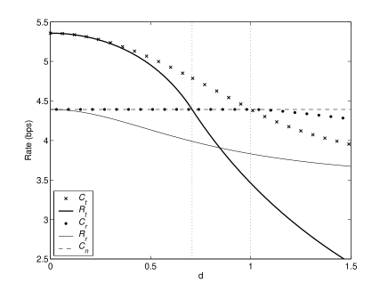
Figure 3: Cut-set bounds and achievable rates in Case 2.

Case 3: Optimal power allocation with receiver phase CSI

When remote phase information is not available, it was derived in [12, 9] that it is optimal to set $\rho=0$ in the cut-set bounds (3), (5), and the decode-and-forward transmitter cooperation rate (4). Intuitively, with only receiver phase CSI, the relay and the transmitter, being unable to realize the gain from coherent combining, resort to sending uncorrelated signals.

The receiver cooperation strategy of compress-and-forward, on the other hand, did not make use of remote phase information [12], and so the receiver cooperation rate is still given by (6) with the power allocation parameter $\alpha$ optimally chosen.

Under the transmitter cooperation configuration, the cut-set bound is found to be

$$C^{3}_{t}=\mathcal{C}(1),$$ (17)

where $\alpha^{*}$ is any value in the range $[1/(g+1),1]$. When the relay is close to the transmitter ($g\geq 1$), the decode-and-forward strategy is capacity achieving, as reported in [12]. Specifically, the transmitter cooperation rate is given by

$$R^{3}_{t}=\Bigl{\{}\textstyle\mathcal{C}(1)\text{ if }g\geq 1,\quad\mathcal{C}(g)\text{ if }g<1\Bigr{.},$$ (18)

where $\alpha^{*}$ is any value in the range $[1/g,1]$ if $g\geq 1$, and $\alpha^{*}=1$ otherwise.

For receiver cooperation, the cut-set bound is

$$C^{3}_{r}=\Bigl{\{}\textstyle\mathcal{C}\bigl{(}\frac{2g}{g+1}\bigr{)}\text{ if }g\geq 1,\quad\mathcal{C}(1)\text{ if }g<1\Bigr{.},$$ (19)

where $\alpha^{*}=g/(g+1)$ if $g>1$, $\alpha^{*}=1$ if $g<1$, and $\alpha^{*}$ is any value in the range $[g/(g+1),1]$ if $g=1$. Since compress-and-forward does not require remote phase information, the receiver cooperation rate is the same as (10) given in Case 1: $R^{3}_{r}=R^{1}_{r}$. Note that the argument inside $\mathcal{C}(\cdot)$ in (10) is 1 when $\alpha=1$, and hence $R^{3}_{r}\geq\mathcal{C}(1)$.

In contrast to Case 2, the receiver cooperation rate $R^{3}_{r}$ in equals or outperforms the transmitter cooperation cut-set bound $C^{3}_{t}$; consequently receiver cooperation is the superior strategy when the system is under optimal power allocation with only receiver phase CSI. Numerical examples of the upper bounds and achievable rates are shown in Fig. 4.

Figure 4: Cut-set bounds and achievable rates in Case 3.

Case 4: Equal power allocation with receiver phase CSI

With equal power allocation, $\alpha$ is set to $1/2$. With only receiver phase CSI, similar to Case 3, $\rho=0$ is optimal for the cut-set bounds and decode-and-forward rate. Therefore, in this case no optimization is necessary, and the bounds and achievable rates can be readily evaluated.

For transmitter cooperation, the cut-set bound and the decode-and-forward rate, respectively, are

$$C^{4}_{t} =\Bigl{\{}\textstyle\mathcal{C}(1)\text{ if }g\geq 1,\quad\mathcal{C}\bigl{(}\frac{1+g}{2}\bigr{)}\text{ if }g<1\Bigr{.},$$ (20)

$$R^{4}_{t} =\Bigl{\{}\textstyle\mathcal{C}(1)\text{ if }g\geq 2,\quad\mathcal{C}\bigl{(}\frac{g}{2}\bigr{)}\text{ if }g<2\Bigr{.}.$$ (21)

For receiver cooperation, the cut-set bound is

$$C^{4}_{r}=\Bigl{\{}\textstyle\mathcal{C}(1)\text{ if }g\geq 1,\quad\mathcal{C}\bigl{(}\frac{1+g}{2}\bigr{)}\text{ if }g<1\Bigr{.},$$ (22)

and the compress-and-forward rate is the same as (16) in Case 2: $R^{4}_{r}=R^{2}_{r}$.

Parallel to Case 1, the transmitter and receiver cooperation cut-set bounds $C^{4}_{t}$ and $C^{4}_{r}$ are identical. Note that the non-cooperative capacity $C_{n}$ meets the cut-set bounds when $g\geq 1$, and even beats the bounds when $g<1$. Hence it can be concluded cooperation offers no capacity improvement when the system is under equal power allocation with only receiver phase CSI. Numerical examples are plotted in Fig. 5.

Figure 5: Cut-set bounds and achievable rates in Case 4.

IV Implementation Strategies

In the previous section, for each given operational environment we derived the most advantageous cooperation strategy. The available mode of cooperation is sometimes dictated by practical system constraints, however. For instance, in a wireless sensor network collecting measurements for a single remote base station, only transmitter cooperation is possible. In this section, for a given transmitter or receiver cluster, the trade-off between cooperation capacity gain and implementation complexity is investigated.

The upper bounds and achievable rates from the previous section are summarized, and ordered, in Table III: the rate of an upper row is at least as high as that of a lower one. It is assumed that the cooperating nodes are close together such that $g>2$. The transmitter cooperation rates are plotted in Fig. 6. It can be observed that optimal power allocation contributes only marginal additional capacity gain over equal power allocation, while having full CSI is essential to achieving any cooperative capacity gain. Accordingly, in transmitter cooperation, homogeneous nodes with common battery and amplifier specifications can be employed to simplify network deployment, but synchronous-carrier should be considered necessary.

Cooperation Scheme	Rate
$C^{1}_{t}$, $C^{1}_{r}$	$\mathcal{C}\!\left(\frac{2(g+1)}{g+2}\right)$
$R^{1}_{t}$, $C^{2}_{t}$, $C^{3}_{r}$	$\mathcal{C}\!\left(\frac{2g}{g+1}\right)$
$R^{2}_{t}$	$\mathcal{C}\!\left(\frac{2(g-1)}{g}\right)$
$R^{\prime}_{r}$	$\mathcal{C}\!\left(\frac{2g(\sqrt{g-1}-1)(g-1-\sqrt{g-1})}{\sqrt{g-1}(g-2)^{2}}\right)$
$R^{1}_{r}$, $R^{3}_{r}$	${\displaystyle\max_{0\leq\alpha\leq 1}}\mathcal{C}\!\left(\frac{\alpha(1-\alpha)g}{(1-\alpha)g+2\alpha+1/P}+\alpha\right)$
$C_{n}$, $C^{2}_{r}$, $C^{3}_{t}$, $R^{3}_{t}$, $C^{4}_{t}$, $R^{4}_{t}$, $C^{4}_{r}$	$\mathcal{C}(1)$
$R^{2}_{r}$, $R^{4}_{r}$	$\mathcal{C}\!\left(\frac{g}{2(g+2+2/P)}+\frac{1}{2}\right)$

TABLE III: Cooperation rates comparison

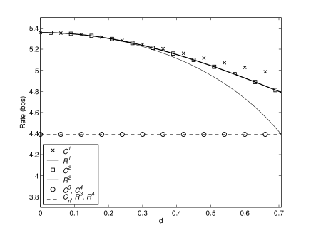
Figure 6: Transmitter Cooperation

On the other hand, in receiver cooperation, the compress-and-forward scheme does not require full CSI, but optimal power allocation is crucial in attaining cooperative capacity gain, as illustrated in Fig. 7. When remote phase information is not utilized (i.e., $\rho=0$), as noted in [7], carrier-level synchronization is not required between the relay and the transmitter; implementation complexity is thus significantly reduced. It is important, however, to allow for the network nodes to have different power requirements and power allocation be optimized among them.

Figure 7: Receiver Cooperation

V Conclusion

We have studied the capacity improvement from transmitter and receiver cooperation when the cooperating nodes form a cluster in a relay network. It was shown that electing the proper cooperation strategy based on the operational environment is a key factor in realizing the benefits of cooperation in an ad-hoc wireless network. When full CSI is available, transmitter cooperation is the preferable strategy. On the other hand, when remote phase information is not available but power can be optimally allocated, the superior strategy is receiver cooperation. Finally, when the system is under equal power allocation with receiver phase CSI only, cooperation offers no capacity improvement over a non-cooperative single-transmitter single-receiver channel under the same average network power constraint.

References

- [1] A. Sendonaris, E. Erkip, and B. Aazhang, “User cooperation diversity—Part I: System description,” IEEE Trans. Commun., vol. 51, no. 11, pp. 1927–1938, Nov. 2003.
- [2] ——, “User cooperation diversity—Part II: Implementation aspects and performance analysis,” IEEE Trans. Commun., vol. 51, no. 11, pp. 1939–1948, Nov. 2003.
- [3] T. E. Hunter and A. Nosratinia, “Cooperation diversity through coding,” in Proc. IEEE Int. Symp. Inform. Theory, 2002.
- [4] J. N. Laneman, D. N. C. Tse, and G. W. Wornell, “Cooperative diversity in wireless networks: Efficient protocols and outage behavior,” IEEE Trans. Inform. Theory, vol. 50, no. 12, pp. 3062–3080, Dec. 2004.
- [5] N. Jindal, U. Mitra, and A. J. Goldsmith, “Capacity of ad-hoc networks with node cooperation,” in Proc. IEEE Int. Symp. Inform. Theory, 2004, also in preparation for IEEE Trans. Inform. Theory.
- [6] C. T. K. Ng and A. J. Goldsmith, “Transmitter cooperation in ad-hoc wireless networks: Does dirty-payer coding beat relaying?” in Proc. IEEE Inform. Theory Workshop, San Antonio, Texas, Oct. 2004.
- [7] A. Host-Madsen, “Capacity bounds for cooperative diversity,” IEEE Trans. Inform. Theory, submitted for publication. [Online]. Available: http://www-ee.eng.hawaii.edu/~madsen/papers
- [8] M. A. Khojastepour, A. Sabharwal, and B. Aazhang, “Improved achievable rates for user cooperation and relay channels,” in Proc. IEEE Int. Symp. Inform. Theory, 2004.
- [9] A. Host-Madsen and J. Zhang, “Capacity bounds and power allocation for wireless relay channel,” IEEE Trans. Inform. Theory, submitted for publication. [Online]. Available: http://www-ee.eng.hawaii.edu/~madsen/papers
- [10] A. Host-Madsen, “On the achievable rate for receiver cooperation in ad-hoc networks,” in Proc. IEEE Int. Symp. Inform. Theory, 2004.
- [11] ——, “A new achievable rate for cooperative diversity based on generalized writing on dirty paper,” in Proc. IEEE Int. Symp. Inform. Theory, 2003.
- [12] G. Kramer, M. Gastpar, and P. Gupta, “Cooperative strategies and capacity theorems for relay networks,” IEEE Trans. Inform. Theory, Feb. 2004, to be published. [Online]. Available: http://cm.bell-labs.com/cm/ms/who/gkr/pub.html
- [13] E. C. van der Meulen, “Three-terminal communication channels,” Adv. Appl. Prob., vol. 3, pp. 120–154, 1971.
- [14] T. M. Cover and A. A. El Gamal, “Capacity theorems for the relay channel,” IEEE Trans. Inform. Theory, vol. 25, no. 5, 1979.
- [15] T. M. Cover and J. A. Thomas, Elements of Information Theory. Wiley-Interscience, 1991.
- [16] A. D. Wyner and J. Ziv, “The rate-distortion function for source coding with side information at the decoder,” IEEE Trans. Inform. Theory, vol. 22, no. 1, pp. 1–10, Jan. 1976.