Multiresolution Kernels

Abstract

We present in this work a new methodology to design kernels on data which is structured with smaller components, such as text, images or sequences. This methodology is a template procedure which can be applied on most kernels on measures and takes advantage of a more detailed “bag of components” representation of the objects. To obtain such a detailed description, we consider possible decompositions of the original bag into a collection of nested bags, following a prior knowledge on the objects’ structure. We then consider these smaller bags to compare two objects both in a detailed perspective, stressing local matches between the smaller bags, and in a global or coarse perspective, by considering the entire bag. This multiresolution approach is likely to be best suited for tasks where the coarse approach is not precise enough, and where a more subtle mixture of both local and global similarities is necessary to compare objects. The approach presented here would not be computationally tractable without a factorization trick that we introduce before presenting promising results on an image retrieval task.

1 Introduction

There is strong evidence that kernel methods [11] can deliver state-of-the-art performance on most classification tasks when the input data lies in a vector space. Arguably, two factors contribute to this success. First, the good ability of kernel algorithms, such as the SVM, to generalize and provide a sparse formulation for the underlying learning problem; Second, the capacity of nonlinear kernels, such as the polynomial and RBF kernels, to quantify meaningful similarities between vectors, notably non-linear correlations between their components. Using kernel machines with non-vectorial data (e.g., in bioinformatics, pattern recognition or signal processing tasks) requires more arbitrary choices, both to represent the objects and to chose suitable kernels on those representations. The challenge of using kernel methods on real-world data has thus recently fostered many proposals for kernels on complex objects, notably for strings, trees, images or graphs to cite a few.

A strategy often quoted as the generative approach to this problem takes advantage of a generative model, that is an adequate statistical model for the objects, to derive feature representations for the objects. In practice this often yields kernels to be used on the histograms of smaller components sampled in the objects, where the kernels take into account the geometry of the underlying model in their similarity measures [7, 9, 4, 6, 3]. The previous approaches coupled with SVM’s combine both the advantages of using discriminative methods with generative ones, and produced convincing results on many tasks.

One of the drawbacks of such representations is however that they implicitly assume that each component has been generated independently and in a stationary way, where the empirical histogram of components is seen as a sample from an underlying stationary measure. While this viewpoint may translate into adequate properties for some learning tasks (such as translation or rotation invariance when using histograms of colors to manipulate images [2]), it might prove too restrictive and hence inadequate for other types of problems. Namely, tasks which involve a more subtle mix of detecting both conditional (with respect to the location of the components for instance) and global similarities between the objects. Such problems are likely to arise for instance in speech, language, time series or image processing. In the first three tasks, this consideration is notably treated by most state-of-the-art methods through dynamic programming algorithms capable of detecting and penalizing accordingly local matches between the objects. Using dynamic programming to produce a kernel yielded fruitful results in different applications [14, 12], with the limitation that the kernels obtained in practice are not always positive definite, as reviewed in [14]. Other kernels proposed for sequences [10] directly incorporate a localization information into each component, augmenting considerably the size of the component space, and then introduce some smoothing (such as mismatches) to avoid representations that would be too sparse.

Figure 1: From the bag of components representation to a set of nested bags, using a set of conditioning events.

We propose in this work a different approach grounded on the generative approach previously quoted, managing however to combine both conditional and global similarities when comparing two objects. The motivation behind this approach is both intuitive and computational: intuitively, the global histogram of components, that is the simple bag of components representation of Figure 1, may seem inadequate if the components’ appearance seem to be clearly conditioned by some external events. This phenomenon can be taken into account by considering collections (indexed on the same set of events, to be defined) of nested bags or histograms to describe the object. Kernels that would only rely on these detailed resolutions might however miss the bigger picture that is provided by the global histogram. We propose a trade-off between both viewpoints through a combination that aims at giving a balanced account of both fine and coarse perspectives, hence the name of multiresolution kernels, which we introduce formally in Section 2. On the computational side, we show how such a theoretical framework can translate into an efficient factorization detailed in Section 3. We then provide experimental results in Section 4 on an image retrieval task which shows that the methodology improves the performance of kernel based state-of-the art techniques in this field.

2 Multiresolution Kernels

In most applications, complex objects can be represented as histograms of components, such as texts as bags of words or images and sequences as histograms of colors and letters. Through this representation, objects are cast as probability laws or measures on the space $\mathcal{X}$ of components, typically multinomials if $\mathcal{X}$ is finite  [9, 6, 2, 8], and compared as such through kernels on measures. An obvious drawback of this representation is that all contextual information on how the components have been sampled is lost, notably any general sense of position in the objects, but also more complex conditional information that may be induced from neighboring components, such as transitions or long range interactions.

In the case of images for instance, one may be tempted to consider not only the overall histogram of colors, but also more specialized histograms which may be relevant for the task. If some local color-overlapping in the images is an interesting or decisive feature of the learning problem, these specialized histograms may be generated arbitrarily following a grid, dividing for instance the image into 4 equal parts, and computing histograms for each corner before comparing them pairwise between two images (see Figure 2 for an illustration). If sequences are at stake, these may also be sliced into predefined regions to yield local histograms of letters. If the strings are on the contrary assumed to follow some Markovian behaviour (namely that the appearance of letters in the string is independent of their exact location but only depends on the few letters that precede them), an interesting index would translate into a set of contexts, typically a complete suffix dictionary as detailed in [4]. While the two previous examples may seem opposed in the way the histograms are generated, both methodologies stress a particular class of events (location or transitions) that give an additional knowledge on how the components were sampled in the objects. Since both these two approaches, and possibly other ones, can be applied within the framework of this paper using a unified formalism, we present our methodology using a general notation for the index of events. Namely, we note $\mathcal{T}$ for an arbitrary set of conditioning events, assuming these events can be directly observed on the object itself, by contrast with the latent variables approach of  [13]. Considering still, following the generative approach, that an object can be mapped onto a probability measure $\mu$ on $\mathcal{X}$, we have that the realization of an event $t\operatorname{\in\,}\mathcal{T}$ can be interpreted under the light of a joint probability $\mu(x,t)$, with $x\operatorname{\in\,}\mathcal{X}$, factorized through Bayes’ law as $\mu(x|t)\mu(t)$ to yield the following decomposition of $\mu$ as

$$\mu=\sum_{t\operatorname{\in\,}\mathcal{T}}\mu_{t},$$

where each $\mu_{t}\operatorname{\overset{\operatorname{def}}{=}}\mu(\cdot|t)\mu(t)$ is an element of the set of sub-probability measures $M_{+}^{s}(\mathcal{X})$, that is the set of positive measures $\rho$ on $\mathcal{X}$ such that their total mass $\rho(\mathcal{X})$ denoted as $|\rho|$ is less than or equal to $1$. To take into account the information brought by the events in $\mathcal{T}$, objects can hence be represented as families of measures of $M_{+}^{s}(\mathcal{X})$ indexed by $\mathcal{T}$, namely elements $\mu$ contained in $M_{\mathcal{T}}(\mathcal{X})\overset{\operatorname{def}}{=}M_{+}^{s}(\mathcal{X})^{\mathcal{T}}.$

2.1 Local Similarities Between Measures Conditioned by Sets of Events

To compare two objects under the light of their respective decompositions as sub-probability measures $\mu_{t}$ and $\mu_{t}^{\prime}$, we make use of an arbitrary positive definite kernel $k$ on $M_{+}^{s}(\mathcal{X})$ to which we will refer to as the base kernel throughout the paper. For interpretation purposes only, we may assume in the following sections that $k$ can be written as $e^{-d^{2}}$ where $d$ is an Euclidian distance in $M_{+}^{s}(\mathcal{X})$. Note also that the kernel is defined not only on probability measures, but also on sub-probabilities. For two elements $\mu,\mu^{\prime}$ of $M_{\mathcal{T}}(\mathcal{X})$ and a given element $t\operatorname{\in\,}\mathcal{T}$, the kernel

$$k_{t}(\mu,\mu^{\prime})\overset{\operatorname{def}}{=}k(\mu_{t},\mu^{\prime}_{t})$$

measures the similarity of $\mu$ and $\mu^{\prime}$ by quantifying how similarly their components were generated conditionally to event $t$. For two different events $s$ and $t$ of $\mathcal{T}$, $k_{s}$ and $k_{t}$ can be associated through polynomial combinations with positive factors to result in new kernels, notably their sum $k_{s}+k_{t}$ or their product $k_{s}k_{t}$. This is particularly adequate if some complementarity is assumed between $s$ and $t$, so that their combination can provide new insights for a given learning task. If on the contrary the events are assumed to be similar, then they can be regarded as a unique event $\{s\}\cup\{t\}$ and result in the kernel

$$k_{\{s\}\cup\{t\}}(\mu,\mu^{\prime})\operatorname{\overset{\operatorname{def}}{=}}k(\mu_{s}+\mu_{t},\mu^{\prime}_{s}+\mu^{\prime}_{t}),$$

which will measure the similarity of $m$ and $m^{\prime}$ when either $s$ or $t$ occurs. The previous formula can be extended to model kernels indexed on a set $T\subset\mathcal{T}$ of similar events, through

$$k_{T}(m,m^{\prime})\operatorname{\overset{\operatorname{def}}{=}}k\left(\mu_{T},\mu^{\prime}_{T}\right),\;\text{where }\;\mu_{T}\operatorname{\overset{\operatorname{def}}{=}}\sum_{t\operatorname{\in\,}T}{\mu_{t}}\;\text{ and }\;\mu^{\prime}_{T}\operatorname{\overset{\operatorname{def}}{=}}\sum_{t\operatorname{\in\,}T}{\mu^{\prime}_{t}}.$$

Note that this equivalent to defining a distance between elements $\mu$ and $\mu^{\prime}$ conditionned by $T$ as $d^{2}_{T}(\mu,\mu^{\prime})\operatorname{\overset{\operatorname{def}}{=}}d^{2}(\mu_{T},\mu^{\prime}_{T})$.

2.2 Resolution Specific Kernels

Let $P$ be a finite partition of $\mathcal{T}$, that is a finite family $P=(T_{1},...,T_{n})$ of sets of $\mathcal{T}$, such that $T_{i}\cap T_{j}=\varnothing$ if $1\leq i<j\leq n$ and $\bigcup_{i=1}^{n}T_{i}=\mathcal{T}$. We write $\mathcal{P}(\mathcal{T})$ for the set of all partitions of $\mathcal{T}$. Consider now the kernel defined by a partition $P$ as

$$k_{P}(\mu,\mu^{\prime})\operatorname{\overset{\operatorname{def}}{=}}\prod_{i=1}^{n}k_{T_{i}}(\mu,\mu^{\prime}).$$ (1)

The kernel $k_{P}$ quantifies the similarity between two objects by detecting their joint similarity under all possible events of $\mathcal{T}$, given an a priori similarity assumed on the events which is expressed as a partition of $\mathcal{T}$. Note that there is some arbitrary in this definition since, following the convolution kernels [5] approach for instance, a simple multiplication of base kernels $k_{T_{i}}$ to define $k_{P}$ is used, rather than any other polynomial combination. More precisely, the multiplicative structure of Equation (1) quantifies how two objects are similar given a partition $P$ in a way that imposes for the objects to be similar according to all subsets $T_{i}$. If $k$ can be expressed as a function of a distance $d$, $k_{P}$ can be expressed as the exponential of

$$d^{2}_{P}(\mu,\mu^{\prime})\operatorname{\overset{\operatorname{def}}{=}}\sum_{i=1}^{n}d^{2}_{T_{i}}(\mu,\mu^{\prime}),$$

a quantity which penalizes local differences between the decompositions of $\mu$ and $\mu^{\prime}$ over $\mathcal{T}$, as opposed to the coarsest approach where $P=\{\mathcal{T}\}$ and only $d^{2}(\mu,\mu^{\prime})$ is considered.

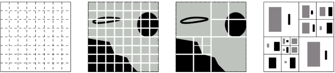
Figure 2: A useful set of events $\mathcal{T}$ for images which would focus on pixel localization can be represented by a grid, such as the $8\times 8$ one represented above. In this case $P_{3}$ corresponds to the $4^{3}$ windows presented in the left image, $P_{2}$ to the $16$ larger square obtained when grouping $4$ small windows, $P_{1}$ to the image divided into $4$ equal parts and $P_{0}$ is simply the whole image. Any partition of the image obtained from sets in $P_{0}^{3}$, such as the one represented above, can in turn be used to represent an image as a family of sub-probability measures, which reduces in the case of two-color images to binary histograms as illustrated in the right-most image.

As illustrated in Figure 2 in the case of images expressed as histograms indexed over locations, a partition of $\mathcal{T}$ reflects a given belief on how events should be associated to belong to the same set or dissociated to highlight interesting dissimilarities. Hence, all partitions contained in the set $\mathcal{P}(\mathcal{T})$ of all possible partitions are not likely to be equally meaningful given that some events may look more similar than others. If the index is based on location, one would naturally favor mergers between neighboring indexes. For contexts, a useful topology might also be derived by grouping contexts with similar suffixes.

Such meaningful partitions can be obtained in a general case if we assume the existence of a prior hierarchical information on the elements of $\mathcal{T}$, translated into a series

$$P_{0}=\{\mathcal{T}\},..,P_{D}=\{\{t\},t\operatorname{\in\,}\mathcal{T}\}$$

of partitions of $\mathcal{T}$, namely a hierarchy on $\mathcal{T}$. To provide a hierarchical content, the family $(P_{d})_{d=1}^{D}$ is such that any subset present in a partition $P_{d}$ is included in a (unique by definition of a partition) subset included in the coarser partition $P_{d-1}$, and further assume this inclusion to be strict. This is equivalent to stating that each set $T$ of a partition $P_{d}$ is divided in $P_{d+1}$ through a partition of $T$ which is not $T$ itself. We note this partition $s(T)$ and name its elements the siblings of $T$. Consider now the subset $\mathcal{P}_{D}\subset\mathcal{P}(\mathcal{T})$ of all partitions of $\mathcal{T}$ obtained by using only sets in

$$P_{0}^{D}\overset{\operatorname{def}}{=}\bigcup_{d=1}^{D}P_{d},$$

namely $\mathcal{P}_{D}\overset{\operatorname{def}}{=}\{P\operatorname{\in\,}\mathcal{P}(\mathcal{T})\text{ s.t. }\forall\,T\operatorname{\in\,}P,T\operatorname{\in\,}P_{0}^{D}\}.$. The set $\mathcal{P}_{D}$ contains both the coarsest and the finest resolutions, respectively $P_{0}$ and $P_{D}$, but also all variable resolutions for sets enumerated in $P_{0}^{D}$, as can be seen for instance in the third image of Figure 2.

2.3 Averaging Resolution Specific Kernels

Each partition $P$ contained in $\mathcal{P}_{D}$ provides a resolution to compare two objects, and generates consequently a very large family of kernels $k_{P}$ when $P$ spans $\mathcal{P}_{D}$. Some partitions are probably better suited for certain tasks than others, which may call for an efficient estimation of an optimal partition given a task. We take in this section a different direction by considering an averaging of such kernels based on a Bayesian prior on the set of partitions. In practice, this averaging favours objects which share similarities under a large collection of resolutions.

Definition 1.

Let $\mathcal{T}$ be an index set endowed with a hierarchy $(P_{d})_{d=0}^{D}$, $\pi$ be a prior measure on the corresponding set of partitions $\mathcal{P}_{D}$ and $k$ a base kernel on $M_{+}^{s}(\mathcal{X})\times M_{+}^{s}(\mathcal{X})$. The multiresolution kernel $k_{\pi}$ on $M_{\mathcal{T}}(\mathcal{X})\times M_{\mathcal{T}}(\mathcal{X})$ is defined as

$$k_{\pi}(\mu,\mu^{\prime})=\sum_{P\operatorname{\in\,}\mathcal{P}_{D}}\pi(P)\,k_{P}(\mu,\mu^{\prime}).$$ (2)

Note that in Equation (2), each resolution specific kernel contributes to the final kernel value and may be regarded as a weighted feature extractor.

3 Kernel Computation

This section aims at characterizing hierarchies $(P_{d})_{d=0}^{D}$ and priors $\pi$ for which the computation of $k_{\pi}$ is both tractable and meaningful. We first propose a type of hierarchy generated by trees, which is then coupled with a branching process prior to fully specify $\pi$. These settings yield a computational time for expressing $k_{\pi}$ which is loosely upperbounded by $D\times\operatorname{card}{\mathcal{T}}\times c(k)$ where $c(k)$ is the time required to compute the base kernel.

3.1 Partitions Generated by Branching Processes

All partitions $P$ of $\mathcal{P}_{D}$ can be generated iteratively through the following rule, starting from the initial root partition $P:=P_{0}=\{\mathcal{T}\}$. For each set $T$ of $P$:

1. either leave the set as it is in $P$,

2. either replace it by its siblings enumerated in $s(T)$, and reapply this rule to each sibling unless they belong to the finest partition $P_{D}$.

By giving a probabilistic content to the previous rule through a binomial parameter (i.e. for each treated set assign probability $1-\varepsilon$ of applying rule 1 and probability $\varepsilon$ of applying rule 2) a candidate prior for $\mathcal{P}_{D}$ can be derived, depending on the overall coarseness of the considered partition. For all elements $T$ of $P_{D}$ this binomial parameter is equal to $0$, whereas it can be individually defined for any element $T$ of the $D-1$ coarsest partitions as $\varepsilon_{T}\operatorname{\in\,}[0,1]$, yielding for a partition $P\operatorname{\in\,}\mathcal{P}_{D}$ the weight

$$\pi(P)=\prod_{T\operatorname{\in\,}P}(1-\varepsilon_{T})\prod_{T\operatorname{\in\,}\overset{\circ}{P}}(\varepsilon_{T}),$$

where the set $\overset{\circ}{P}=\{T\operatorname{\in\,}P_{0}^{D}\text{ s.t. }\exists V\operatorname{\in\,}P,V\subsetneq T\}$ gathers all coarser sets belonging to coarser resolutions than $P$, and can be regarded as all ancestors in $P_{0}^{D}$ of sets enumerated in $P$.

3.2 Factorization

The prior proposed in Section 3.1 can be used to factorize the formula in (2), which is summarized in this theorem, using notations used in Definition 1

Theorem 1.

For two elements $m,m^{\prime}$ of $M_{\mathcal{T}}(\mathcal{X})$, define for $T$ spanning recursively $P_{D},P_{D-1},...,P_{0}\,$ the quantity

$$K_{T}=(1-\varepsilon_{T})k_{T}(\mu,\mu^{\prime})+\varepsilon_{T}\prod_{U\operatorname{\in\,}\,s(T)}K_{U}.$$

Then $k_{\pi}(\mu,\mu^{\prime})=K_{\mathcal{T}}$.

Proof.

The proof follows from the prior structure used for the tree generation, and can be found in either [1] or [4]. Figure 3 underlines the importance of incorporating to each node $K_{T}$ a weighted product of the kernels $K_{U}$ computed by its siblings. ∎

Figure 3: The update rule for the computation of $k\pi$ takes into account the branching process prior by updating each node corresponding to a set $T$ of any intermediary partitions with the values obtained for higher resolutions in $s(T)$.

If the hierarchy of $\mathcal{T}$ is such that the cardinality of $s(T)$ is fixed to a constant $\alpha$ for any set $T$, typically $\alpha=4$ for images as seen in Figure 2, then the computation of $k_{\pi}$ is upperbounded by $(\alpha^{D+1}-1)c(k)$. This computational complexity may even become lower in cases where the histograms become sparse at fine resolutions, yielding complexities in linear time with respect to the size of the compared objects, quantified by the length of the sequences in [4] for instance.

4 Experiments

We present in this section experiments inspired by the image retrieval task first considered in [2] and also used in [6], although the images used here are not exactly the same. The dataset was also extracted from the Corel Stock database and includes 12 families of labelled images, each class containing 100 color images, each image being coded as $256\times 384$ pixels with colors coded in 24 bits (16M colors). The families depict bears, African specialty animals, monkeys, cougars, fireworks, mountains, office interiors, bonsais, sunsets, clouds, apes and rocks and gems. The database is randomly split into balanced sets of 900 training images and 300 test images. The task consists in classifying the test images with the rule learned by training 12 one-vs-all SVM’s on the learning fold. The object are then classified according to the SVM performing the highest score, namely with a “winner-takes-all” strategy. The results presented in this section are averaged over 4 different random splits. We used the CImg package to generate histograms and the Spider toolbox for the SVM experiments.

We adopted a coarser representation of 9 bits per color for the $98,304$ pixels of each image, rather than the 24 available ones to reduce the size of the RGB color space to $8^{3}=512$ from the original set of $256^{3}=16,777,216$ colors. In this image retrieval experiment, we used localization as the conditioning index set, dividing the images into $1,4,4^{2}=16,9$ and $9^{2}=81$ local histograms (in Figure 2 the image was for instance divided into $4^{3}=64$ windows). To define the branching process prior, we simply set an uniform value over all the grid of $\varepsilon$ of $1/\alpha$, an usage motivated by previous experiments led in a similar context [4]. Finally, we used kernels described in both [2] and [6] to define the base kernel $k$. These kernels can be directly applied on sub-probability measures, which is not the case for all kernels on multinomials, notably the Information Diffusion Kernel [9]. We report results for two families of kernels, namely the Radial Basis Function expressed for multinomials and the entropy kernel based on the Jensen divergence [6, 3]:

$$k_{a,b,\rho}(\theta,\,\theta^{\prime})=e^{-\rho\sum|\theta_{i}^{a}-{\theta^{\prime}_{i}}^{a}|^{b}}\;\;,\;k_{h}(\theta,\,\theta^{\prime})=e^{-h\left(\frac{\theta+\theta^{\prime}}{2}\right)+\frac{1}{2}\left(h(\theta)+h(\theta^{\prime})\right)}.$$

For most kernels not presented here, the multiresolution approach usually improved the performance in a similar way than the results presented in Table 1. Finally, we also report that using only the finest resolution available in each $(\alpha,D)$ setting, that is a branching process prior uniformly set to $1$, yielded better results than the use of the coarsest histogram without achieving however the same performance of the multiresolution averaging framework, which highlights the interest of taking both coarse and fine perspectives into account. When $a=.25$ for instance, this setting produced 16.5% and 16.2% error rates for $\alpha=4$ and $D=1,2$, and 15.8% for $\alpha=9$ and $D=1$.

Kernel	RBF, $b=1$, $\rho=.01$			JD
	$a=.25$	$a=.5$	$a=1$
global histogram	18.5	18.3	18.3	21.4
$D=1,\alpha=4$	15.4	16.4	18.8	17
$D=2,\alpha=4$	13.9	13.5	15.8	15.2
$D=1,\alpha=9$	14.7	14.7	16.6	15
$D=2,\alpha=9$	15.1	15.1	30.5	15.35

Table 1: Results for the Corel image database experiment in terms of error rate, with 4 fold cross-validation and 2 different types of tested kernels, the RBF and the Jensen Divergence.

References

- [1] Olivier Catoni. Statistical learning theory and stochastic optimization, Ecole d’été de probabilités de Saint-Flour XXXI -2001. Number 1851 in Lecture Notes in Mathematics. Springer Verlag, 2004.
- [2] O. Chapelle, P. Haffner, and V. Vapnik. Svms for histogram based image classification. IEEE Transactions on Neural Networks, 10(5):1055, September 1999.
- [3] Marco Cuturi, Kenji Fukumizu, and Jean-Philippe Vert. Semigroup kernels on measures. Journal of Machine Learning Research, 6:1169–1198, 2005.
- [4] Marco Cuturi and Jean-Philippe Vert. The context-tree kernel for strings. Neural Networks, 18(8), 2005.
- [5] David Haussler. Convolution kernels on discrete structures. Technical report, UC Santa Cruz, 1999. USCS-CRL-99-10.
- [6] M. Hein and O. Bousquet. Hilbertian metrics and positive definite kernels on probability measures. January 2005.
- [7] Tony Jebara, Risi Kondor, and Andrew Howard. Probability product kernels. Journal of Machine Learning Research, 5:819–844, 2004.
- [8] Thorsten Joachims. Learning to Classify Text Using Support Vector Machines: Methods, Theory, and Algorithms. Kluwer Academic Publishers, Dordrecht, 2002.
- [9] John Lafferty and Guy Lebanon. Diffusion kernels on statistical manifolds. Journal of Machine Learning Research, 6:129–163, January 2005.
- [10] G. Rätsch and S. Sonnenburg. Accurate splice site prediction for caenorhabditis elegans. In Bernhard Schölkopf, Koji Tsuda, and Jean-Philippe Vert, editors, Kernel Methods in Computational Biology. MIT Press, 2004.
- [11] Bernhard Schölkopf and Alexander J. Smola. Learning with Kernels: Support Vector Machines, Regularization , Optimization, and Beyond. MIT Press, Cambridge, MA, 2002.
- [12] H. Shimodaira, K.-I. Noma, M. Nakai, and S. Sagayama. Dynamic time-alignment kernel in support vector machine. In T. G. Dietterich, S. Becker, and Z. Ghahramani, editors, Advances in Neural Information Processing Systems 14, Cambridge, MA, 2002. MIT Press.
- [13] K. Tsuda, T. Kin, and K. Asai. Marginalized kernels for biological sequences. Bioinformatics, 18(Suppl 1):268–275, 2002.
- [14] Jean-Philippe Vert, Hiroto Saigo, and Tatsuya Akutsu. Local alignment kernels for protein sequences. In Bernhard Schölkopf, Koji Tsuda, and Jean-Philippe Vert, editors, Kernel Methods in Computational Biology. MIT Press, 2004.