Comparison of two different implementations of a finite-difference-method for first-order pde in Mathematica${}^{\textrm{\textregistered}}$ and Matlab${}^{\textrm{\textregistered}}$

Abstract

In this article two implementations of a symmetric finite difference algorithm (ftcs-method) for a first-order partial differential equation are discussed. The considered partial differential equation discribes the time evolution of the crack length ditribution of microcracks in brittle materia.

1 Physics and analytical solution

The growth rate of microcracks in a brittle material can be discribed by a mesoscopic equation. Here the specialized version for uniaxial loading is presented.

$$\frac{\partial f(l,t)}{\partial t} = -\frac{1}{l^{2}}\frac{\partial l^{2}v_{l}(l,t)f(l,t)}{\partial l},$$ (1)

$f(l,t)$ is the distribution function for the crack length $l$ at time $t$, $v_{l}=\dot{l}$ is the growth velocity of the cracks. A Rice-Griffith-like dynamic is assumed for crack growth, which gives

$$\dot{l} = \begin{cases}-\alpha^{\prime}+\beta^{\prime}l\sigma(t)^{2}&\textrm{, if }\alpha^{\prime}\leq\beta^{\prime}l\sigma^{2}\\ 0&\textrm{, otherwise}\end{cases}$$ (2)

The theory is given in detail in [1]. For an exponential (or a step-wise) initial condition and constant loading speed it is possible to give an exact analytical solution, which is also presented in [1] and looks like:

$$f(l,t) = \begin{cases}l^{-2}e^{-\frac{\beta^{\prime}v_{\sigma}^{2}}{3}t^{3}}F\left(le^{-\frac{\beta^{\prime}v_{\sigma}^{2}}{3}t^{3}}+\frac{\alpha^{\prime}}{(9\beta^{\prime}v_{\sigma}^{2})^{1/3}}\Gamma(1/3,0,\frac{\beta^{\prime}v_{\sigma}^{2}}{3}t^{3})\right)&\textrm{, if}\quad\alpha^{\prime}\leq\beta^{\prime}v_{\sigma}^{2}lt^{2}\\ &\\ f(l,0)&\textrm{, otherwise}.\end{cases}$$ (3)

(a) step-wise initial condition

(b) step-wise initial condition

(c) exponential initial condition

Figure 1: Analytical solution for crack lenght distributuion. Shown is $f(l,t)l^{2}$ over $l$ and $t$.

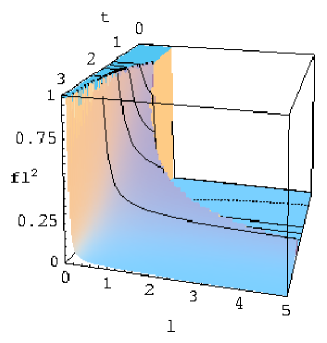
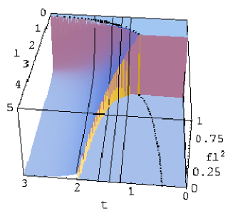
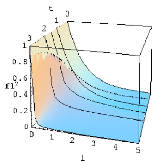
2 The numerical algorithm

The partial differential equations are first order in time and crack length. Two different algorithms, upwind and fcts (forward time centered space), have been tested. The symmetric algorithm (ftcs-method) is in this case a bit more stable than the upwind, which is somewhat astonishing. Both algorithms can be found in [2].
In the symmetric algorithm $f(l,t+1)$ is calculated from $f(l-1,t)$, $f(l,t)$ and $f(l+1,t)$ by

$$f(l,t+1) = f(l,t)\left(1-\left(3\beta\sigma^{2}(t)-\frac{2\alpha}{dl\ l})dt\right)-\left(dl\ l\beta\sigma^{2}(t)\right)-\alpha\right)\times$$ (4)

$$\times\frac{dt}{2dl}\left(f(l+1,t)-f(l-1,t)\right)$$

This is what the main part of the implementation in Mathematica${}^{\textrm{\textregistered}}$ looks like:

For[t = 1, t < TMAX, t++, For[l = 1, l < LMAX, l++,
   If[l*dl*(t*dt)^2*be - al > 0,
    If[l == 0, f[l, t + 1] = f[l, t],
     f[l, t + 1] =
          f[l, t]*(1 - (3*be*(t*dt)^2 - (2*al)/(dl*l))*dt) -
          (dl*l*be*(t*dt)^2 - al)*dt/dl*(f[l + 1, t] - f[l - 1, t])],
    f[l, t + 1] = f[l, t]
    ]
   ]
]

This is what the main part of the implementation in Matlab${}^{\textrm{\textregistered}}$ looks like:

for t=1:1:TMAX-1
  for l=1:1:LMAX-1
    if (l.*dl.*sigma(t).*beta-alpha > 0)
      f(l,t+1)=f(l,t).*(1-(3.*beta.*(sigma(t)).^2 - ...
(2.*alpha)./(dl.*l)).*dt)-(dl.*l.*beta.*(sigma(t)).^2 - ...
alpha).*dt./(2*dl).*(f(l+1,t)-f(l-1,t));
    else
    f(l,t+1)=f(l,t);
    end
  end
end

3 Results obtained by Mathematica${}^{\textrm{\textregistered}}$

Mathematica${}^{\textrm{\textregistered}}$ is a general purpose computer algebra system (cas) by Wolfram Research Inc..

(a) step-wise initial condition

(b) exponential initial condition

Figure 2: Numerical solution for crack lenght distributuion calculated with Mathematica${}^{\textrm{\textregistered}}$

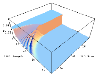
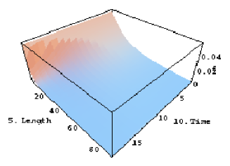
As one can see the solution shows some wave-like efects, which can be interpreted as a sign for numerical instability. This instability is a result of the discontinous initial condition.

4 Results obtained by Matlab${}^{\textrm{\textregistered}}$

Matlab${}^{\textrm{\textregistered}}$ is a tool for numerical mathematics, especially designed for matrix manipulation, by The MathWorks Inc..

(a) step-wise initial condition

(b) exponential initial condition

Figure 3: Numerical solution for crack lenght distributuion calculated with Matlab${}^{\textrm{\textregistered}}$

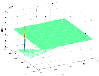
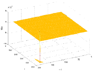
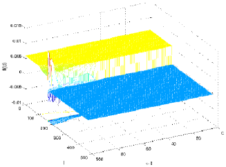
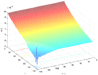
Here in both cases huge instabilities occur. As soon as some cracks start growing the numerical error goes to infinity. The following pictures show an extract of the above pictures.

(a) step-wise initial condition

(b) exponential initial condition

Figure 4: Numerical solution for crack lenght distributuion calculated with Matlab${}^{\textrm{\textregistered}}$ (extract of figure 3)

5 Comparison of the results and conclusion

Obviously the results, obtained with both programs, show huge errors. But in contrast to the results calculated with Matlab${}^{\textrm{\textregistered}}$ , one can use the results obtained with Mathematica${}^{\textrm{\textregistered}}$ at least for some rough predictions.
The difference in the two software packages, used for these simulations, is that Matlab${}^{\textrm{\textregistered}}$ uses floating-point variables of precision “double” (16 byte), whereas Mathematica${}^{\textrm{\textregistered}}$ is capable of both numerical and symolic computation. Therefore it is possible that Mathematica${}^{\textrm{\textregistered}}$ uses a much higher precision to perform some of the operations than Matlab${}^{\textrm{\textregistered}}$ .

References

- [1] P. Ván, C. Papenfuss, and W. Muschik. Griffith cracks in the mesoscopic microcrack theory. Journal of Physics A, 37(20):5315–5328, 2004. (cond-mat/0211207).
- [2] W. H. Press, S. A. Teukolsky, W. T Vetterling, and B. P. Flannery. Numerical Recipes in C. Cambridge University Press, Cambridge, USA, 1994.