A Unified Framework for Tree Search Decoding: Rediscovering the Sequential Decoder

Abstract

We consider receiver design for coded transmission over linear Gaussian channels. We restrict ourselves to the class of lattice codes and formulate the joint detection and decoding problem as a closest lattice point search (CLPS). Here, a tree search framework for solving the CLPS is adopted. In our framework, the CLPS algorithm decomposes into the preprocessing and tree search stages. The role of the preprocessing stage is to expose the tree structure in a form matched to the search stage. We argue that the minimum mean square error decision feedback (MMSE-DFE) frontend is instrumental for solving the joint detection and decoding problem in a single search stage. It is further shown that MMSE-DFE filtering allows for using lattice reduction methods to reduce complexity, at the expense of a marginal performance loss, and solving under-determined linear systems. For the search stage, we present a generic method, based on the branch and bound (BB) algorithm, and show that it encompasses all existing sphere decoders as special cases. The proposed generic algorithm further allows for an interesting classification of tree search decoders, sheds more light on the structural properties of all known sphere decoders, and inspires the design of more efficient decoders. In particular, an efficient decoding algorithm that resembles the well known Fano sequential decoder is identified. The excellent performance-complexity tradeoff achieved by the proposed MMSE-Fano decoder is established via simulation results and analytical arguments in several MIMO and ISI scenarios.

1 Introduction

Recent years have witnessed a growing interest in the closest lattice point search (CLPS) problem. This interest was primarily sparked by the connection between CLPS and maximum likelihood (ML) decoding in multiple-input multiple-output (MIMO) channels [12]. On the positive side, MIMO channels offer significant advantages in terms of increased throughput and reliability. The price entailed by these gains, however, is a more challenging decoding task for the receiver. For example, naive implementations of the ML decoder have complexity that grows exponentially with the number of transmit antennas. This observation inspired several approaches for sub-optimal decoding that offer different performance-complexity tradeoffs (e.g., [3, 26]).

Reduced complexity decoders are typically obtained by exploiting the codebook structure. The scenario considered in our work is no exception. In principle, the decoders considered here exploit the underlying lattice structure of the received signal to cast the decoding problem as a CLPS. Some variants of such decoders are known in the literature as sphere decoders (e.g., [14, 34, 1, 30, 45]). These decoders typically exploit number-theoretic ideas to efficiently span the space of allowed codewords (e.g., [23, 42]). The complexity of such decoders were shown, via simulation and numerical analysis, to be significantly smaller than the naive ML decoder in many scenarios of practical interest (e.g., [14, 34]). The complexity of the state of the art sphere decoder, however, remains prohibitive for problems characterized by a large dimensionality [36]. This observation is one of the main motivations for our work.

The overriding goal of our work is to establish a general framework for the design and analysis of tree search algorithms for joint detection and decoding. Towards this goal, we first divide the decoding task into two interrelated stages; namely, 1) preprocessing and 2) tree search. The preprocessing stage is primarily concerned with exposing the underlying tree structure from the noisy received signal. Here, we discuss the integral roles of minimum mean square error decision feedback (MMSE-DFE) filtering, lattice reduction techniques, and relaxing the boundary control (i.e., lattice decoding) in tree search decoding. We then proceed to the search stage where a general framework based on the branch and bound (BB) algorithm is presented. This framework establishes, rigorously, the equivalence in terms of performance and complexity between different sphere and sequential decoders. We further use the proposed framework to classify the different search algorithms and identify their advantages/disadvantages. The MMSE-Fano decoder emerges as a special case of our general framework that enjoys a favorable performance-complexity tradeoff. We establish the superiority of the proposed decoder via numerical results and analytical arguments in several relevant scenarios corresponding to coded as well as uncoded transmission over MIMO and inter-symbol-interference (ISI) channels. More specifically, in our simulation experiments, we apply the tree search decoding framework to uncoded V-BLAST [27], linear dispersion space-time codes [33], algebraic space-time codes [31, 41, 40], and trellis codes over ISI channels [17]. In all these cases, our results show that the MMSE-Fano decoder achieves near-ML performance with a much smaller complexity.

The rest of the paper is organized as follows. Section 2 introduces our system model and notation. In Section 3, we consider the design of the preprocessing stage and discuss the interplay between this stage and the tree search stage. In Section 4, we present a general framework for designing tree search decoders based on the branch and bound (BB) algorithm. In Section 5, we establish the superior performance-complexity tradeoff achieved by the proposed MMSE-Fano decoder, using analytical arguments and numerical results, in several interesting scenarios. Finally, we offer some concluding remarks in Section 6

2 System Model

We consider the transmission of lattice codes over linear channels with white Gaussian additive noise (AWGN). The importance of this problem stems from the fact that several very relevant applications arising in digital communications fall in this class, as it will be illustrated by some examples at the end of this section. Let $\Lambda\subseteq\mbox{\bb R}^{m}$ be an $m$-dimensional lattice, i.e., the set of points

$$\Lambda=\{\hbox{\boldmath$\lambda$}={\bf G}{\bf x}\;:\;{\bf x}\in\mbox{\bb Z}^{m}\}$$ (1)

where ${\bf G}\in\mbox{\bb R}^{m\times m}$ is the lattice generator matrix. Let ${\bf v}\in\mbox{\bb R}^{m}$ be a vector and ${\cal R}$ a measurable region in $\mbox{\bb R}^{m}$. A lattice code ${\cal C}(\Lambda,{\bf v},{\cal R})$ is defined [24, 25, 18] as the set of points of the lattice translate $\Lambda+{\bf v}$ inside the shaping region ${\cal R}$, i.e.,

$${\cal C}(\Lambda,{\bf v},{\cal R})=\{\Lambda+{\bf v}\}\cap{\cal R}.$$ (2)

Without loss of generality, we can also see ${\cal C}(\Lambda,{\bf v},{\cal R})$ as the set of points ${\bf c}+{\bf v}$, such that the codewords ${\bf c}$ are given by

$${\bf c}={\bf G}{\bf x},\;\;\;\mbox{for}\;\;{\bf x}\in{\cal U}$$ (3)

where ${\cal U}\subset\mbox{\bb Z}^{m}$ is the code information set.

The linear additive noise channel is described, in general, by the input-output relation

$$\mathbf{r=H(c+v)+z}$$ (4)

where ${\bf r}\in\mbox{\bb R}^{n}$ denotes the received signal vector, ${\bf z}\sim{\cal N}({\bf 0},{\bf I})$ is the AWGN vector, and ${\bf H}\in{\mathbb{R}}^{n\times m}$ is a matrix that defines the channel linear mapping between the input and the output.

Consider the following communication problem: a vector of information symbols ${\bf x}$ is generated with uniform probability over ${\cal U}$, the corresponding codeword ${\bf c}={\bf G}{\bf x}$ is produced by the encoder and the signal ${\bf c}+{\bf v}$ is transmitted over the channel (4). Assuming ${\bf H}$ and ${\bf v}$ known to the receiver, the ML decoding rule is given by

$$\hat{\mathbf{x}}=\textrm{arg}\min_{{\mathbf{x}}\in{\mathcal{U}}}|{\mathbf{r}}-{{\bf H}}{{\bf v}}-{\mathbf{H}}{\bf G}{\mathbf{x}}|^{2}$$ (5)

The constraint ${\mathcal{U}}\subset{\mathbb{Z}}^{m}$ implies that the optimization problem in (5) can be viewed as a constrained version of the CLPS with lattice generator matrix given by ${\mathbf{H}}{\bf G}$ and constraint set ${\cal U}$.

A few remarkable examples of the above framework are:

1. MIMO flat fading channels: One of the simplest and most widely studied examples is a MIMO V-BLAST system with squared QAM modulation, $M$ transmit and $N$ receive antennas, operating over a flat Rayleigh fading channel. The baseband complex received signal in this case can be expressed as

   $${\mathbf{r}}^{c}=\sqrt{\frac{\rho}{M}}{\mathbf{H}}^{c}\mathbf{c}^{c}+\mathbf{z}^{c}$$ (6)

   where the complex channel matrix ${\mathbf{H}}^{c}\in{\mathbb{C}}^{N\times M}$ is composed of i.i.d elements $h_{i,j}^{c}\sim{\mathcal{N}}_{\mathcal{C}}(0,1)$, the input complex signal ${\mathbf{c}}^{c}$ has components ${\mathbf{c}}_{i}^{c}$ chosen from a unit-energy $Q^{2}$-QAM constellation, the noise has i.i.d. components $z^{c}_{i}\sim{\cal N}_{{\cal C}}(0,1)$ and $\rho$ denotes the signal to noise ratio (SNR) observed at any receive antenna. The system model in (6) can be expressed in the form of (4) by appropriate scaling and by separating the real and imaginary parts using the vector and the matrix transformations defined by

   $${\bf u}^{c}\mapsto{\bf u}=[{\rm Re}\{{\bf u}^{c}\}^{{}^{T}},{\rm Im}\{{\bf u}^{c}\}^{{}^{T}}]^{{}^{T}},$$

   $${\mathbf{M}}^{c}\mapsto{\bf M}=\left[\begin{array}[]{cc}{\rm Re}\{{\bf M}^{c}\}&-{\rm Im}\{{\bf M}^{c}\}\\ {\rm Im}\{{\bf M}^{c}\}&{\rm Re}\{{\bf M}^{c}\}\end{array}\right].$$

   The resulting real model is given by (4) where $n=2N$, $m=2M$ and the constraint set is given by ${\cal U}=\mbox{\bb Z}_{Q}^{m}$, with $\mbox{\bb Z}_{Q}=\{0,\ldots,Q-1\}$ denoting the set of integers residues modulo $Q$.

   In the case of V-BLAST, the lattice code generator matrix ${\bf G}=\kappa{\bf I}$, where $\kappa$ is a normalizing constant, function of $Q$, that makes the (complex) transmitted signal of unit energy per symbol. This formulation extends naturally to MIMO channels with more general lattice coded inputs [18]. In general, a space-time code of block length $T$ is defined by a set of matrices ${\bf C}^{c}=[{\bf c}^{c}_{1},\ldots,{\bf c}^{c}_{T}]$ in $\mbox{\bb C}^{M\times T}$. The columns of the codeword ${\bf C}^{c}$ are transmited in parallel on the $M$ transmit antennas in $T$ channel uses. The received signal is given by the sequence of vectors

   $${\mathbf{r}}^{c}_{t}=\sqrt{\frac{\rho}{M}}{\mathbf{H}}^{c}\mathbf{c}^{c}_{t}+\mathbf{z}^{c}_{t},\;\;\;t=1,\ldots,T$$ (7)

   Lattice space-time codes are obtained by taking a lattice code ${\cal C}(\Lambda,{\bf v},{\cal R})$ in $\mbox{\bb R}^{2MT}$, and mapping each codeword ${\bf c}$ into a complex matrix ${\bf C}^{c}$ according to some linear one-to-one mapping $\mbox{\bb R}^{2MT}\rightarrow\mbox{\bb C}^{M\times T}$. It is easy to see that a lattice-coded MIMO system can be again expressed by (4) where the channel matrix ${\bf H}$ is proportional (through an appropriate scaling factor) to the block-diagonal matrix

   $${\bf I}_{T}\otimes\left[\begin{array}[]{cc}{\rm Re}\{\mathbf{H}^{c}\}&-{\rm Im}\{\mathbf{H}^{c}\}\\ {\rm Im}\{\mathbf{H}^{c}\}&{\rm Re}\{\mathbf{H}^{c}\}\end{array}\right]$$ (8)

   In this case, we have $n=2NT$ and $m=2MT$. It is interesting to notice that for a wide class of linear dispersion (LD) codes [33, 19, 13, 5, 43], the information set ${\cal U}$ is still given by $\mbox{\bb Z}_{Q}^{m}$, as in the simple V-BLAST case, although the generator matrix ${\bf G}$ is generally not proportional to ${\bf I}$. For other classes of lattice codes [18], with more involved shaping regions ${\cal R}$, the information set ${\cal U}$ does not take on the simple form of an “hypercube”. For example, consider $\Lambda$ obtained by construction A [10], i.e., $\Lambda=C+Q\mbox{\bb Z}^{m}$, where $C\subseteq\mbox{\bb Z}_{Q}^{m}$ is a linear code over $\mbox{\bb Z}_{Q}$ with generator matrix in systematic form $[{\bf I},{\bf P}^{{}^{T}}]^{{}^{T}}$. A generator matrix of $\Lambda$ is given by [10]

   $${\bf G}=\left[\begin{array}[]{cc}{\bf I}&{\bf 0}\\ {\bf P}&Q{\bf I}\end{array}\right].$$ (9)

   Typically, the shaping region ${\cal R}$ of the lattice code ${\cal C}(\Lambda,{\bf v},{\cal R})$ can be an $m$-dimensional sphere, the fundamental Voronoi region of a sublattice $\Lambda^{\prime}\subset\Lambda$, or the $m$-dimensional hypercube. In all these cases, the information set ${\cal U}$ may be difficult to describe.

2. ISI Channels: For simplicity, we consider a baseband real single-input single-output (SISO) inter-symbol-interference (ISI) channel with the input and output sequences related by

   $${r_{i}=\sum_{\ell=0}^{L}h_{\ell}c_{i-\ell}+z_{i}},$$

   where $(h_{0},\ldots,h_{L})$ denotes the discrete-time channel impulse response, assumed of finite length $L+1$. The extension to the complex baseband model is immediate. Assuming that the transmitted signal is padded by $L$ zeroes, the channel can be written in the form (4) where the channel matrix takes on the tall banded Toeplitz form

   $$\mathbf{H}=\left[\begin{array}[]{cccc}h_{0}&&&\\ h_{1}&h_{0}&&\\ \vdots&\ddots&\ddots&\\ h_{L}&\ddots&\ddots&h_{0}\\ &h_{L}&\ddots&h_{1}\\ &&\ddots&\vdots\\ &&&h_{L}\\ \end{array}\right].$$

   A wide family of trellis codes obtained as coset-codes [24, 25], including binary linear codes, can be formulated as lattice codes where $\Lambda$ is a Construction A lattice and the shaping region ${\cal R}$ is chosen appropriately. In particular, coded modulation schemes based on the $Q$-PAM constellation obtained by mapping group codes over $\mbox{\bb Z}_{Q}$ onto the $Q$-PAM constellation can be seen as lattice codes with hypercubic shaping ${\cal R}$. The important case of binary convolutional codes falls in this class for $Q=2$. Again, the information set ${\cal U}$ corresponding to ${\cal R}$ may, in general, be very complicated.

3 The Preprocessing Stage

In our framework, we divide the CLPS into two stages; namely, 1) preprocessing and 2) tree search. The complexity and performance of CLPS algorithms depend critically on the efficiency of the preprocessing stage. Loosely, the goal of preprocessing is to transform the original constrained CLPS problem, described by the lattice generator matrix ${\bf H}{\bf G}$ and by the constraint set ${{\cal U}}$, into a form which is friendly to the search algorithm used in the subsequent stage. In the following, we discuss the different tasks performed in the preprocessing stage. In general, a friendly tree structure can be exposed through three steps: left preprocessing, right preprocessing, and forming the tree.

Some options for these three steps are illustrated in the following subsections. However, before entering the algorithmic details, it is worthwhile to point out some general considerations. The classical sphere decoding approach to the solution of the original constrained CLPS problem (5) consists of applying QR decomposition on the combined channel and code matrix, i.e., letting ${\bf H}{\bf G}={\bf Q}{\bf R}$ where ${\bf Q}\in\mbox{\bb R}^{n\times m}$ has orthonormal columns and ${\bf R}\in\mbox{\bb R}^{m\times m}$ is upper triangular. Using the fact that ${\bf Q}^{{}^{T}}$ is an isometry with respect to the Euclidean distance, (5) can be written as

$$\hat{\mathbf{x}}=\textrm{arg}\min_{{\mathbf{x}}\in{\mathcal{U}}}\Big{|}{\mathbf{y}}^{\prime}-{\bf R}{\bf x}\Big{|}^{2}$$ (10)

where ${\bf y}^{\prime}={\bf Q}^{{}^{T}}({\bf r}-{\bf H}{\bf v})$. If rank$({\bf H}{\bf G})=m$, ${\bf R}$ has non-zero diagonal elements and its triangular form can be exploited to search for all the points ${\bf x}\in{\cal U}$ such that ${\bf R}{\bf x}$ is in a sphere of a given search radius centered in ${\bf y}^{\prime}$. If the sphere is non-empty, the ML solution is guaranteed to be found inside the sphere, otherwise, the search radius is increased and the search is restarted. Different variations on this main theme have been proposed in the literature, and will be reviewed in Section 4 as special cases of a general BB algorithm. Nevertheless, it is useful to point out here the two main sources of inefficiency of the above approach: 1) It does not apply to the case rank$({\bf H}{\bf G})<m$ and, even when rank$({\bf H}{\bf G})=m$ but ${\bf H}{\bf G}$ is ill-conditioned, the spread (or dynamic range) of the diagonal elements of ${\bf R}$ is large. This entails large complexity of the tree search [15]. Intuitively, when ${\bf H}{\bf G}$ is ill-conditioned, the lattice generated by ${\bf H}{\bf G}$ has a very skewed fundamental cell such that there are directions in which it is very difficult to distinguish the points $\{{\bf H}{\bf G}{\bf x}:{\bf x}\in{\cal U}\}$; 2) Enforcing the condition ${\bf x}\in{\cal U}$, can be very difficult because a lattice code ${\cal C}(\Lambda,{\bf v},{\cal R})$ with non-trivial shaping region ${\cal R}$ might have an information set ${\cal U}$ with a complicated shape. Hence, just checking the condition ${\bf x}\in{\cal U}$ during the search may entail a significant complexity.

Left preprocessing can be seen as an effort to tackle the first problem: it modifies the channel matrix and the noise vector such that the resulting CLPS problem is non-equivalent to ML (therefore, it is suboptimal), but it has a much better conditioned “channel” matrix. The second problem can be tackled by relaxing the constraint set ${\cal U}$ to the whole $\mbox{\bb Z}^{m}$, i.e., searching over the whole lattice $\Lambda$ instead of only the lattice code ${\cal C}$ (or lattice decoding). In general, lattice decoding is another source of suboptimality. Nevertheless, once the boundary region is removed, we have the freedom of choosing the lattice basis which is more convenient for the search algorithm. This change of lattice basis is accomplished by right preprocessing. Finally, the tree structure is obtained by factorizing the resulting combined channel-lattice matrix in upper triangular form, as in classical sphere decoding. Overall, left and right preprocessing combined with lattice decoding are a way to reduce complexity at the expense of optimality. Fortunately, it turns out that an appropriate combination of these elements yields very significant saving in complexity with very small degradation with respect to the ML performance. Thus, it yields a very attractive decoding solution. While the outstanding performance of appropriate preprocessing and lattice decoding can be motivated via rigorous information theoretic arguments [18, 21, 20], here we are more concerned with the algorithmic aspects of the decoder and we shall give some heuristic motivation based on “signal-processing” arguments.

Finally, we note that the notion of complexity adopted in this work does not capture the complexity of the preprocessing stage (mostly cubic in the lattice dimension). In practice, this assumption is justified in slowly varying channels where the complexity of the preprocessing stage will be shared by many transmission frames (e.g., a wired ISI channel or a wireless channel with stationary terminals). If the number of these frames is large enough, i.e., the channel is slow enough, the preprocessing complexity can be ignored compared to the complexity of the tree search stage which has to be independently performed in every frame. Optimizing the complexity of the preprocessing stage, however, is an important topic, especially for fast fading channels.

3.1 Taming the Channel: Left Preprocessing

In the case of uncoded transmission (${\bf G}={\bf I}$), QR decomposition of the channel matrix ${\bf H}$ (assuming rank$({\bf H})=m$) allows simple recursive detection of the information symbols ${\bf x}$. Indeed, ${{\bf Q}}$ is the feedforward matrix of the zero-forcing decision feedback equalizer (ZF-DFE) [27]. In general, sphere decoders can be seen as ZF-DFEs with some reprocessing capability of their tentative decisions.

It is well-known that ZF-DFE is outperformed by the MMSE-DFE in terms of signal-to-interference plus noise ratio (SINR) at the decision point, under the assumption of correct decision feedback [8]. This observation motivates the proposed approach for left preprocessing [15]. This new matrix can be obtained through the QR decomposition of the augmented channel matrix

$$\tilde{{\bf H}} {\,\,\stackrel{{\scriptstyle\scriptscriptstyle\bigtriangleup}}{{=}}\,\,} \left[\begin{array}[]{c}{\bf H}\\ {\bf I}\\ \end{array}\right]=\tilde{{\bf Q}}{\bf R}_{1}$$ (13)

where $\tilde{{\bf Q}}\in\mbox{\bb R}^{(n+m)\times m}$ has orthonormal columns and ${\bf R}_{1}$ is upper triangular. Let ${\bf Q}_{1}$ be the upper $n\times m$ part of $\tilde{{\bf Q}}$. ${{\bf Q}}_{1}$ and ${{\bf R}}_{1}$ are the MMSE-DFE forward and backward filters, respectively. Thus, the transformed channel matrix and the received sequence are given by ${\bf R}_{1}$ and ${\bf y}^{\prime}=({\mathbf{Q}}_{1}^{{}^{T}}{{\bf r}}-{\bf R}_{1}{\bf v})$, respectively. The transformed CLPS

$$\min_{{\bf x}\in{\cal U}}\Big{|}{\mathbf{y}}^{\prime}-{\bf R}_{1}{\bf G}{\bf x}\Big{|}^{2}$$ (14)

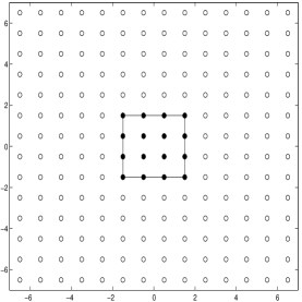
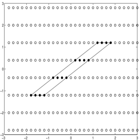
(a) The translated $\mbox{\bb Z}^{2}$ lattice and QAM constellation	(b) The received lattice after channel distortion (constellation)
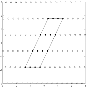
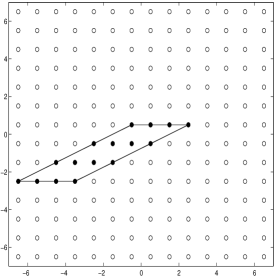
(c) After MMSE-DFE left preprocessing	(d) Boundary control after right preprocessing

Figure 2: The effect of left preprocessing on the lattice and the right preprocessing on the information set

is not equivalent to (5) since, in general, ${\bf Q}_{1}$ does not have orthonormal columns. The additive noise ${\bf w}={\bf y}^{\prime}-{\bf R}_{1}{\bf G}{\bf x}$ in (14) contains both a Gaussian component, given by ${\bf Q}_{1}^{{}^{T}}{\bf z}$, and a non-Gaussian (signal-dependent) component, given by $({\bf Q}_{1}^{{}^{T}}{\bf H}-{\bf R}_{1})({\bf c}+{\bf v})$. Nevertheless, for lattice codes such that cov$({\bf c}+{\bf v})={\bf I}$, it can be shown that cov$({\bf w})={\bf I}$ [18]. Hence, the additive noise component ${\bf w}$ in (14) is still white, although non-Gaussian and data dependent. Therefore, the minimum distance rule (14) is expected to be only slightly suboptimal. On the other hand, the augmented channel matrix $\widetilde{{\bf H}}$ in (13) has always rank equal to $m$ and it is well conditioned, since ${\bf R}_{1}^{{}^{T}}{\bf R}_{1}={\bf I}+{\bf H}^{{}^{T}}{\bf H}$. Therefore, in some sense we have tamed the channel at the (small) price of the non-Gaussianity of the noise. The better conditioning achieved by the MMSE-DFE preprocessing is illustrated in Fig.2 (b) and (c).

3.2 Inducing Sparsity: Right Preprocessing

In order to obtain the tree structure, one needs to put $\mathbf{R}_{1}{\bf G}$ in upper triangular form ${\bf R}$ via QR decomposition. The sparser the matrix ${\mathbf{R}}$, the smaller the complexity of the tree search algorithm. For example, a diagonal ${\mathbf{R}}$ means that symbol-by-symbol detection is optimal, i.e., the tree search reduces to exploring a single path in the tree. Loosely, if one adopts a depth first search strategy, then a sparse ${\mathbf{R}}$ will lead to a better quality of the first leaf node found by the algorithm. Consequently, the algorithm finds the closest point in a shorter time [14].

While we have no rigorous method for relating the “sparsity” of ${\bf R}$ to the complexity of the tree search, inspired by decision feedback equalization in ISI channel, we define the sparsity index of the upper triangular matrix $\mathbf{R}$ as follows

$${\textsf{S}}({\bf R}) {\,\,\stackrel{{\scriptstyle\scriptscriptstyle\bigtriangleup}}{{=}}\,\,} \max_{i\in\{1,\ldots,m\}}\frac{\sum_{j=i+1}^{m}r_{i,j}^{2}}{r_{i,i}^{2}}.$$ (15)

where $r_{i,j}$ denotes the $(i,j)$-th element of ${\bf R}$. One can argue that the smaller ${\textsf{S}}({\bf R})$ the sparser ${\bf R}$ (e.g., ${\textsf{S}}({\bf R})=0$ for ${\bf R}$ diagonal). The goal of right preprocessing is to find a change of basis of the lattice $\{{\bf R}_{1}{\bf G}{\bf x}:{\bf x}\in\mbox{\bb Z}^{m}\}$, such that the new lattice generator matrix, ${\bf S}$, satisfies ${\bf S}={\bf Q}{\bf R}$ with ${\textsf{S}}({\bf R})$ as small as possible. This amounts to finding a unimodular matrix ${\bf T}$ (i.e., the entries of $\mathbf{T}$ and ${\mathbf{T}}^{-1}$ are integers) such that ${\bf R}_{1}{\bf G}={\bf Q}{\bf R}{\bf T}$ with ${\bf Q}$ unitary and ${\textsf{S}}({\bf R})$ minimized over the group of unimodular matrices. This optimization problem appears very difficult to solve; however, there exist many heuristic approaches to find unimodular matrices that give small values of ${\textsf{S}}({\bf R})$. Examples of such methods, considered here, are lattice reduction, column permutation and a combination thereof.

Lattice reduction finds a reduced lattice basis, i.e., the columns of the reduced generator matrix $\mathbf{S}$ have “minimal” norms and are as orthogonal as possible. The most widely used reduction algorithm is due to Lenstra, Lenstra and Lovász (LLL) [39] and has a polynomial complexity in the lattice dimension. An enhanced version of the LLL algorithm, namely the deep insertion modification, was later proposed by Schnorr and Euchner [42]. LLL with deep insertion gives a reduced basis with significantly shorter vectors [9]. In practice, the complexity of the LLL with deep insertion is similar to the original one even though it is an exponential time algorithm in the worst case sense [9].

Another method for decreasing ${\textsf{S}}({\bf R})$ consists of ordering the columns of ${\bf R}_{1}{\bf G}$, i.e., by right-multiplication by a permutation matrix $\Sigma$. In the sequel, we shall use the V-BLAST greedy ordering strategy proposed in [27, 6]. This algorithm finds a permutation matrix $\Sigma$ such that ${\bf R}_{1}{\bf G}={\bf Q}{\bf R}\hbox{\boldmath$\Sigma$}$ maximizes $\min_{i}r_{i,i}^{2}$. Since ${\bf R}^{{}^{T}}{\bf R}=\hbox{\boldmath$\Sigma$}^{-}{{{}^{T}}}{\bf G}^{{}^{T}}{\bf R}_{1}^{{}^{T}}{\bf R}_{1}{\bf G}\hbox{\boldmath$\Sigma$}^{-1}$, i.e., the set $\{\sum_{j}r_{i,j}^{2}\;:\;i=1,\ldots,m\}$ depends only on ${\bf R}_{1}{\bf G}$ and not on $\Sigma$, by maximizing the minimum $r^{2}_{i,i}$ this algorithm miminizes ${\textsf{S}}({\bf R})$ over the group of permutation matrices (a subgroup of the unimodular matrices).

Lattice reduction and column permutation can be combined. This yields an unimodular matrix ${\bf T}=\hbox{\boldmath$\Sigma$}{\bf T}_{1}$, where ${\bf T}_{1}$ is obtained by lattice-reducing ${\bf R}_{1}{\bf G}$ and $\Sigma$ by applying the V-BLAST greedy algorithm on the resulting reduced matrix ${\bf R}_{1}{\bf G}{\bf T}_{1}^{-1}$.

As observed before, the unimodular right multiplication does not change the lattice but may significantly complicate the boundary control. In fact, we have

$$\min_{{\bf x}\in{\cal U}}\Big{|}{\mathbf{y}}^{\prime}-{\bf R}_{1}{\bf G}{\bf x}\Big{|}^{2} = \min_{{\bf x}\in{\cal U}}\Big{|}{\mathbf{y}}^{\prime}-{\bf Q}{\bf R}{\bf T}{\bf x}\Big{|}^{2}$$ (16)

$$= \min_{{\bf x}\in{\bf T}{\cal U}}\Big{|}{\bf Q}^{{}^{T}}{\mathbf{y}}^{\prime}-{\bf R}{\bf x}\Big{|}^{2}$$

The new constraint set ${\bf T}{\cal U}$ might be even more complicated to enforce than the original information set ${\cal U}$ (see Fig. 2(d)). However, it is clear that although modifying the boundary control may result in a significant complexity increase for ML decoding, lattice decoding is not affected at all, since ${\bf T}\mbox{\bb Z}^{m}=\mbox{\bb Z}^{m}$.

3.3 Forming the Tree

The final step in preprocessing is to expose the tree structure of the problem. In this step, QR decomposition is applied on the transformed combined channel and lattice matrix ${\bf Q}_{1}^{{}^{T}}{\bf H}{\bf G}{\bf T}^{-1}$, after left and right preprocessing. The upper triangular nature of ${\mathbf{R}}$ means that a tree search can now be used to solve the CLPS problem. Fig. 1 illustrates an example of such a tree.

Here, we wish to stress that our approach for exposing the tree is fundamentally different from the one traditionally used for codes over finite alphabets (e.g., linear block codes, convolutional codes, trellis coset codes in AWGN channels). Here, we operate over the field of real numbers and consider the lattice corresponding to the joint effect of encoding and channel distortion. In the conventional approach, the tree is generated from the trellis structure of the code alone, and hence, does not allow for a natural tree search that handles jointly detection (the linear channel) and decoding. In fact, joint detection and decoding is achieved at the expenses of an increase of the overall system memory (joint trellis), or by neglecting some paths in the search (e.g., by per-survivor reduced state processing). Since operating on the full joint trellis is usually too complex, both the proposed and the conventional per-survivor (reduced state) approach are suboptimal, and the matter is to see which one achieves the best performance/complexity tradeoff.

For the sake of convenience, in the following we shall denote again by ${\bf y}$ the channel output after all transformations, i.e., the tree search is applied to the CLPS problem $\min_{{\bf x}\in\mbox{\bb Z}^{m}}|{\bf y}-{\bf R}{\bf x}|^{2}$ with ${\bf R}$ in upper triangular form. The components of vectors and matrices are numbered in reverse order, so that the preprocessed received signal can finally be written as

$$\left(\begin{array}[]{c}y_{m}\\ \vdots\\ y_{1}\end{array}\right)=\left(\begin{array}[]{cccc}r_{m,m}&\ldots&\ldots&r_{m,1}\\ 0&r_{m-1,m-1}&\ldots&r_{m-1,1}\\ \vdots&\ddots&\ddots&\vdots\\ 0&\ldots&0&r_{1,1}\end{array}\right)\left(\begin{array}[]{c}x_{m}\\ \vdots\\ x_{1}\end{array}\right)+\left(\begin{array}[]{c}w_{m}\\ \vdots\\ w_{1}\end{array}\right).$$ (17)

Notice that after preprocessing the problem is always squared, of dimension $m$, even though the original problem has arbitrary $m$ and $n$. Throughout the paper, we consider a tree rooted at a fixed dummy node $x_{0}$. The node at level $k$ is denoted by the label ${\mathbf{x}}_{1}^{k}=(x_{1},x_{2},...,x_{k})$. Moreover, every node ${\bf x}_{1}^{k}$ is associated with the the squared distance

$$w_{k}({{\bf x}}_{1}^{k})=\left|y_{k}-\sum_{j=1}^{k}r_{k,j}x_{j}\right|^{2}.$$ (18)

The difference between the transmitted codeword $\hat{\mathbf{x}}$ and any valid codeword ${\mathbf{x}}$ is denoted by $\tilde{\mathbf{x}}$, i.e., $\tilde{\mathbf{x}}=\hat{\mathbf{x}}-{\mathbf{x}}$.

We hasten to stress that the preprocessing steps highlighted in Sections 3.1-3.3 are for a general setting. In some special cases, some steps can be eliminated or alternative options can be used. Some of these cases are listed hereafter.

1. Upper Triangular Code Generator Matrix:
   In this case, after taming the channel, $\mathbf{H}\longrightarrow\mathbf{R}_{1}$, the new combined matrix $\mathbf{R}_{1}\mathbf{G}$ is also upper triangular and can be directly used to form the tree without any further preprocessing (if one decides against right preprocessing).

2. Uncoded V-BLAST:
   For uncoded V-BLAST systems (i.e., $\mathbf{G}=\mathbf{I}$), applying the MMSE-DFE greedy ordering of [32, 6] may achieve better complexity of the tree search stage than applying MMSE-DFE left preprocessing, lattice reduction, and greedy ordering of the final QR decomposition. This is especially true for large dimensions, where lattice reduction is less effective [14].

3. The Hermite Normal Form Transformation:
   Ultimately, any hardware implementation of the decoder requires finite arithmetics. In this case, all quantities are scaled and quantized such that they take on integer values. While all the preprocessing steps in Sections 3.1-3.3 can be easily adapted to finite arithmetics, there exist other efficient transformations for integral matrices that may yield smaller complexity over the ones mentioned above. For example, one can apply the Hermite normal form (HNF) [9] directly on the scaled (and quantized) matrix $\tau{\bf H}{\bf G}$, such $\tau{\bf H}{\bf G}={\bf R}{\bf T}$, with ${\bf T}$ unimodular and ${\bf R}$ upper triangular with the property that each diagonal element dominates the rest of the entries on the same row (i.e., $r_{i,i}>r_{i,j}\geq 0,\,i=1,\ldots,m,\,j=i+1,\ldots,m$). Interestingly, the HNF transformation improves the sparsity index and reduces the preprocessing to a single step.

4 The Tree Search Stage

After proper preprocessing, the second stage of the CLPS corresponds to an instance of searching for the best path in a tree. In this setting, the tree has a maximum depth $m$, and the goal is to find the node(s) at level $m$ that has the least squared distance, where the squared distance for any node ${\mathbf{x}}_{1}^{m}$ at level $m$ (called leaf node) is given by

$$d^{2}({{\bf x}},{{\bf x}}_{1}^{m}) = \sum_{i=1}^{m}w_{i}({{\bf x}}_{1}^{i})$$ (19)

Visiting all leaf nodes to find the one with the least metric, is either prohibitively complex (exponential in $m$), or not possible, as with lattice decoding. The complexity of tree search can be reduced by the branch and bound (BB) algorithm which determines if an intermediate node ${\mathbf{x}}_{1}^{k}$, on extending, has any chance of yielding the desired leaf node. This decision is taken by comparing the cost function assigned to the node by the search algorithm, against a bounding function. In the following section, we propose a generic tree search stage, inspired by the BB algorithm, that encompasses many known algorithms for CLPS as its special cases. We further use this algorithm to classify various tree search algorithms and elucidate some of their structural properties.

4.1 Generic Branch and Bound Search Algorithm

Before describing the proposed algorithm, we first need to introduce some more notation.

• ACTIVE is an ordered list of nodes.

• $f({\mathbf{x}}_{1}^{k})\in{\mathbb{R}}$ is the cost function of any node ${\mathbf{x}}_{1}^{k}$ in the tree, and ${\mathbf{t}}\in{\mathbb{R}}^{m\times 1}$ is the bounding function.

• Any node ${\mathbf{x}}_{1}^{k}$ in the search space of the search algorithm is a valid node, if $f({\mathbf{x}}_{1}^{k})<t_{k}$.

• A node is generated by the search algorithm, if the node occupies any position in ACTIVE at some instant during the search.

• “sort” is a rule for ordering the nodes in the list ACTIVE.

• “gen” is a rule defining the order for generating the child nodes of the node being extended.

• $g_{1}$ and $g_{2}$ are rules for tightening the bounding function.

• At any instant, the leaf node with the least distance generated by the search algorithm so far in the search process is stored in $\hat{\mathbf{x}}$.

• We define the search complexity of a tree search algorithm as the number of nodes generated by the algorithm.

• Two search algorithms are said to be equivalent if they generate the same set of nodes.

• A BB algorithm whose solution is guaranteed to be (one of) leaf node(s) with least distance is called an optimal BB algorithm. If the solution is not guaranteed to have the least distance to ${\mathbf{y}}$ among all leaf nodes, then the BB algorithm is a heuristic BB algorithm.

We are now ready to present our generic search algorithm.

GBB($f$, ${\mathbf{t}}$, sort, gen, $g_{1}$, $g_{2}$):

1. Create the empty list ACTIVE, and place the root node in ACTIVE. Set $n_{c}\leftarrow 1$.

2. Let ${\mathbf{x}}_{1}^{k}$ be the top node of ACTIVE.

   If ${\mathbf{x}}_{1}^{k}$ is a leaf node ($k=m$), then

   ${\mathbf{t}}\leftarrow g_{1}({\mathbf{t}},f({\mathbf{x}}_{1}^{m}))$ and $\hat{\mathbf{x}}\leftarrow{\hbox{arg}}\min(\sum_{i=1}^{m}w_{i}({\mathbf{x}}_{1}^{i}),\sum_{i=1}^{m}w_{i}(\hat{\mathbf{x}}_{1}^{i}))$.

   Remove ${\mathbf{x}}_{1}^{m}$ from ACTIVE.

   Go to step 4.

   If ${\mathbf{x}}_{1}^{k}$ is not a valid node, then remove ${\mathbf{x}}_{1}^{k}$ from ACTIVE. Go to step 4.

   If all valid child nodes of ${\mathbf{x}}_{1}^{k}$ have already been generated, then remove ${\mathbf{x}}_{1}^{k}$ from ACTIVE. Go to step 4.

   Generate a valid child node ${\mathbf{x}}_{1}^{k+1}$ of ${\mathbf{x}}_{1}^{k}$, not generated before, according to the order gen, and place it in ACTIVE. Set $n_{c}\leftarrow n_{c}+1$. Set ${\mathbf{t}}\leftarrow g_{2}({\mathbf{t}},n_{c},\mbox{ACTIVE})$. Update $f({\bf x}_{1}^{k}),f({\bf x}_{1}^{k+1})$.

3. Sort the nodes in ACTIVE according to sort.

4. If ACTIVE is empty, then exit. Else, Go to step 2.

In GBB, $g_{1}$ allows one to tighten the bounding function when a leaf node reaches the top of ACTIVE, whereas $g_{2}$ allows for restricting the search space in heuristic BB algorithms. For example, setting

$$g_{2}({\bf t},n_{c,t},\mbox{ACTIVE})=\left[-\infty,-\infty,...,-\infty\right]^{{}^{T}},$$

will force the search algorithm to terminate when the number of nodes generated increases beyond a tolerable limit on the complexity given by $n_{c,t}$. Whenever a leaf node reaches the top of ACTIVE, $\hat{\mathbf{x}}$ is updated if appropriate. Now, we use GBB to classify various tree search algorithms in three broad categories. This classification highlights the structural properties and advantages/disadvantages of the different search algorithms.

4.1.1 Breadth First Search

GBB becomes a Breadth First Search (BrFS) if $g_{1}({\mathbf{t}},f({\mathbf{x}}_{1}^{m}))={\mathbf{t}}$, and the cost function $f$ of any node, once determined, is never updated. Ultimately, all nodes ${\mathbf{x}}_{1}^{k}$ whose cost function along the path ${\mathbf{x}}_{1}^{k}$ does not rise above the bounding function, are generated before the algorithm terminates, unless the $g_{2}$ function removes their parent nodes from ACTIVE. Now, we can establish the equivalence between various sphere/sequential decoders and BrFS.

The first algorithm is the Pohst enumeration strategy reported in [23]. In this strategy, the bounding function ${\mathbf{t}}$ consists of equal components $C_{0}$, where $C_{0}$ is a constant chosen before the start of search, and the cost function of a node ${{\bf x}}_{1}^{k}$ is $f({{\bf x}}_{1}^{k})=\sum_{i=1}^{k}w_{i}({{\bf x}}_{1}^{i})$. Therefore, all nodes ${{\bf x}}_{1}^{k}$ in the search space that satisfy

$$\sum_{i=1}^{k}w_{i}({\mathbf{x}}_{1}^{i})\leq C_{0}$$ (20)

are generated before termination. Generating the child nodes in this strategy is simplified by the following observation. For any parent node ${{\bf x}}_{1}^{k}$, the condition $\displaystyle{\sum_{i=1}^{k+1}w_{i}({{\bf x}}_{1}^{i})\leq C_{0}}$ for the set of generated child nodes implies that the $(k+1)-$th component of the generated child nodes lies in some interval $[a_{0},a_{1}]$. The second example is the statistical pruning (SP) decoder which is equivalent to a heuristic BrFS decoder. Two variations of SP are proposed in [30], the increasing radii (IR) and elliptical pruning (EP) algorithms. The IR algorithm is a BrFS with the bounding function ${\mathbf{t}}=\{t_{1},...,t_{m}\}$, where $t_{k},1\leq k\leq m$ are constants chosen before the start of search. The cost function for any node in IR is the same as in Pohst enumeration. The EP algorithm is given by the bounding function ${\mathbf{t}}=\{1,...,1\}$, and the cost function for the node ${\mathbf{x}}_{1}^{k}$ given by $\displaystyle{f({\mathbf{x}}_{1}^{k})=\sum_{i=1}^{k}\frac{w_{i}({\mathbf{x}}_{1}^{i})}{e_{k}}}$, where $e_{k},1\leq k\leq m$ are constants. More generally, when $g_{2}(.)={\mathbf{t}}$, i.e., $g_{2}$ is not used, the resulting BrFS algorithm is equivalent to the Wozencraft sequential decoder [47] where, depending on the cost function, the decoder can be heuristic or optimal.

The $M$ algorithm [2] and $T$-algorithm [38] are also examples of heuristic BrFS. Here, however, $g_{2}$ serves an important role in restricting the search space. In both algorithms, sort is defined as follows. Any node in ACTIVE at level $k$ is placed above any node at level $k+1$, and nodes in the same level are sorted in ascending order of their cost functions. In the $M$-algorithm, after the first node at level $k+1$ is generated (indicating that all valid nodes at level $k$ have already been generated), $g_{2}$ sets $t_{k}$ to the cost function of the $M$-th node at level $k$ (where $M$ is an initial parameter of the $M$-algorithm). In the $T$-algorithm, $g_{2}$ sets $t_{k}$ to $(f(\bar{\mathbf{x}}_{1}^{k})+T)$, where $\bar{\mathbf{x}}_{1}^{k}$ is the top node at level $k$ in ACTIVE, and $T$ is a parameter of the $T$-algorithm. After $t_{k}$ is tightened in this manner, all nodes in ACTIVE at level $k$, that satisfy $f({\mathbf{x}}_{1}^{k})>t_{k}$ are rendered invalid, and are subsequently removed from ACTIVE.

In general, BrFS algorithms are naturally suited for applications that require soft-outputs, as opposed to a hard decision on the transmitted frame. The reason is that such algorithms output an ordered list of candidate codewords. One can then compute the soft-outputs from this list using standard techniques (e.g., [35],[4]). Here, we note that in the proposed joint detection and decoding framework, soft outputs are generally not needed. Another advantage of BrFS is that the complexity of certain decoders inspired by this strategy is robust against variations in the SNR and channel conditions. For example, the $M$-algorithm has a constant complexity independent of the channel conditions. This property is appealing for some applications, especially those with hard limits on the maximum, rather than average, complexity. On the other hand, decoders inspired by the BrFS strategy usually offer poor results in terms of the average complexity, especially at high SNR. One would expect a reduced average complexity if the bounding function is varied during the search to exploit the additional information gained as we go on. This observation motivates the following category of tree search algorithms.

4.1.2 Depth First Search

GBB becomes a depth first search (DFS) when the following conditions are satisfied. The sorting rule sort orders the nodes in ACTIVE in reverse order of generation, i.e., the last generated node occupies the top of ACTIVE, and

$$g_{1}({\mathbf{t}},f({\mathbf{x}}_{1}^{m}))=\left[\min(t_{1},f({\mathbf{x}}_{1}^{m})),...,\min(t_{m},f({\mathbf{x}}_{1}^{m}))\right]^{{}^{T}}.$$

As in BrFS, the cost function of any node, once generated, remains constant. Even among algorithms within the class of DFS algorithms, other parameters, like gen and $g_{2}$, can significantly alter the search behavior. To illustrate this point, we contrast in the following several sphere decoders which are equivalent to DFS strategies.

The first example of such decoders is the modified Viterbo-Boutros (VB) decoder reported in [14]. In this decoder, $g_{2}({\mathbf{t}},n_{c})={\mathbf{t}}$, and the cost function for any node ${\mathbf{x}}_{1}^{k}$ is $f({\mathbf{x}}_{1}^{k})=\sum_{i=1}^{k}w_{i}({\mathbf{x}}_{1}^{i})$. For any node ${\mathbf{x}}_{1}^{k}$ and its corresponding interval $[a_{0},a_{1}]$ for valid child nodes, the function gen generates the child node with $a_{0}$ as its $(k+1)^{th}$ component first. Our second example is the Schnorr Euchner (SE) search strategy first reported in [1]. This decoder shares the same cost functions and $g_{2}$ with the modified VB decoder, but differs from it in the order of generating the child nodes. For any node ${\mathbf{x}}_{1}^{k}$ and its corresponding interval $[a_{0},a_{1}]$ for the valid child nodes, let $a_{m}{\,\,\stackrel{{\scriptstyle\scriptscriptstyle\bigtriangleup}}{{=}}\,\,}\lfloor\frac{a_{0}+a_{1}}{2}\rceil$ and $\delta{\,\,\stackrel{{\scriptstyle\scriptscriptstyle\bigtriangleup}}{{=}}\,\,}{\hbox{sign}}(w_{k+1}({\mathbf{x}}_{1}^{k+1}))$. Then, the function gen in the SE decoder generates nodes according to the order $\{a_{m},a_{m}+\delta,a_{m}-\delta,a_{m}+2\delta,\ldots\}$.

Due to the adaptive tightening of the bounding function, DFS algorithms have a lower average complexity than the corresponding BrFS algorithms with the same cost functions, especially at high SNR. Another advantage of the DFS approach is that it allows for greater flexibility in the performance-complexity tradeoff through carefully constructed termination strategy. For example, if we terminate the search after finding the first leaf node, i.e., $n_{c}=m$, then we have the MMSE-Babai point decoder [15]. This decoder corresponds to the MMSE-DFE solution aided with the right preprocessing stage. It was shown in [15] that the performance of this decoder is within a fraction of a dB from the ML decoder in systems with small dimensions. The fundamental weakness of DFS algorithms is that the sorting rule is static and does not exploit the information gained thus far to speed up the search process.

4.1.3 Best First Search

GBB becomes a best first search (BeFS) when the following conditions are satisfied. The nodes in ACTIVE are sorted in ascending order of their cost functions, and

$$g_{1}({\mathbf{t}},f({\mathbf{x}}_{1}^{m}))=\left[\min(t_{1},f({\mathbf{x}}_{1}^{m})),\ldots,\min(t_{m},f({\mathbf{x}}_{1}^{m}))\right]^{{}^{T}}.$$

Note that in BeFS, the search can be terminated once a leaf node reaches the top of the list, since this means that all intermediate nodes have cost functions higher than that of this leaf node. Thus, the bounding function is tightened just once in this case. The stack algorithm is an example of BeFS decoder obtained by setting $g_{2}({\mathbf{t}},n_{c})={\mathbf{t}}$, and the cost function of any node in ACTIVE at any instant defined as follows: If ${\bf x}_{1}^{k}$ is a leaf node, then $f({\bf x}_{1}^{k})=-\infty$. Otherwise, we let ${\bf x}_{1,g}^{k+1}$ be the best child node of ${\bf x}_{1}^{k}$ not generated yet, and define $f({\bf x}_{1}^{k})=\sum_{i=1}^{k+1}w_{i}({\bf x}_{1,g}^{k+1})-b(k+1)$, where we refer to $b\in{\mathbb{R}}^{+}$ as the bias. Because of the efficiency of the sorting rule, BeFS algorithms are generally more efficient than the corresponding BrFS and DFS algorithms. This fact is formalized in the following theorems. Theorem 1 establishes the efficiency of the stack decoder with $b=0$ among all known sphere decoders.

Theorem 1

[48] The stack algorithm with $b=0$ generates the least number of nodes among all optimal tree search algorithms.

The following result compares the heuristic stack algorithm, i.e., $b>0$, with a special case of the IR algorithm [30], where the bounding function takes the form $t_{k}=bk+\delta$.

Theorem 2

The IR algorithm with cost function $\{{\bf t}:t_{k}=bk+\delta\}$, generates at least as many nodes as those generated by the stack algorithm when the same bias $b$ is used.

Proof: Appendix C

At this point, it is worth noting that in our definition of search complexity, we count only the number of generated nodes, i.e., nodes that occupy some position in ACTIVE at some instant. In general, this is a reasonable abstraction of the actual computational complexity involved. However, in the stack algorithm, for each node generated, the cost functions of two nodes are updated instead of one; one for the generated node, and one for the parent node. Thus, the comparisons in Theorems 1 and 2 are not completely fair.

Finally, we report the following two advantages offered by the the stack algorithm. First, it offers a natural solution for the problem of choosing the initial radius (or radii), which is commonly encountered in the design of sphere decoders (e.g., [14]). By setting all the components of $\mathbf{t}$ to $\infty$, it is easy to see that we are guaranteed to find the closest lattice point while generating the minimum number of nodes (among all search algorithms that guarantee finding the closest point). Second it allows for a systematic approach for trading-off performance for complexity. To illustrate this point, if we set $b=0$, we obtain the closest point lattice decoder (i.e., best performance but highest complexity). On the other extreme, when $b\rightarrow\infty$, the stack decoder reduces to the MMSE-Babai point decoder discussed in the DFS section (the number of nodes visited is always equal to $m$). In general, for systems with small $m$, one can obtain near-optimal performance with a relatively large values of $b$. As the number of dimensions increases, more complexity must be expended (i.e., smaller values of $b$) to approach the optimal performance.

4.2 Iterative Best First Search

In Section 4.1, our focus was primarily devoted to complexity, defined as the number of nodes visited by the tree search algorithm. Another important aspect is the memory requirement entailed by the search. Straightforward implementation of the GBB algorithm requires maintaining the list ACTIVE, which can have a prohibitively long length in certain application. This motivates the investigation of modified implementations of these search strategies that are more efficient in terms of storage requirements. The BrFS and DFS sphere decoders discussed in Sections 4.1.1 and 4.1.2 lend themselves naturally to storage efficient implementations. Such implementations have been reported in [23, 14, 15, 1, 30].

In order to exploit the complexity reduction offered by BeFS strategy in practice, it is therefore important to seek modified memory-efficient implementations of such algorithms. This can be realized by storing only one node at a time, and allowing nodes to be visited more than once. The search in this case progresses in contours of increasing bounding functions, thus allowing more and more nodes to be generated at each step, finally terminating once a leaf node is obtained. The Fano decoder [22] is the iterative BeFS variation of the stack algorithm. Although the stack algorithm and the Fano decoder, with the same cost functions, generate essentially the same set of nodes [29], the Fano decoder visits some nodes more than once. However, the Fano decoder requires essentially no memory, unlike the stack algorithm. Appendix A provides an algorithmic description of the Fano decoder and a brief description of the relevant parameters. Overall, the proposed decoder consists of left preprocessing (MMSE-DFE) and right preprocessing (combined lattice reduction and greedy ordering), followed by the Fano (or stack) search stage for lattice, not ML, decoding.

5 Analytical and Numerical Results

To illustrate the efficiency and generality of the proposed framework, we utilize it in three distinct scenarios. First, we consider uncoded transmission over MIMO channels (i.e., V-BLAST). Here, we present analytical, as well as simulation, results that demonstrate the excellent performance-complexity tradeoff achieved by the proposed Stack and Fano decoders. Then, we proceed to coded MIMO systems and apply tree search decoding to two different classes of space-time codes. Finally, we conclude with trellis coded transmission over ISI channels.

5.1 The V-BLAST Configuration

Unfortunately, analytical characterization of the performance- complexity tradeoff for sequential/sphere decoders with arbitrary ${\mathbf{H}}{\mathbf{G}}$ and ${\cal U}$ still appears intractable. To avoid this problem, we restrict ourselves in this section to uncoded transmission over flat Rayleigh MIMO channels. In our analysis, we further assume that ZF-DFE pre-processing is used. The complexity reductions offered by the proposed preprocessing stage are demonstrated by numerical results.

Theorem 3

The Stack algorithm and the Fano decoder with any finite bias $b$, achieve the same diversity as the ML decoder when applied to a V-BLAST configuration.

Proof :   Appendix D.

The result shows that the Fano decoder, unlike other heuristic algorithms like nulling-and-canceling, does not lead to a lower diversity than the ML decoder.

Theorem 4

In a V-BLAST system with $Q^{2}$-QAM, the average complexity per dimension of the stack algorithm for a sufficiently large bias $b$ is linear in $m$ when the SNR $\rho$ grows linearly with $m$ and $r=n-m\geq 0$.

Proof :   Appendix E.

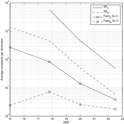
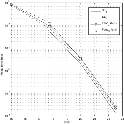
Figure 3: Complexity and Performance of SE enumeration and Fano decoder for a $20\times 20$ $16-$QAM V-BLAST system

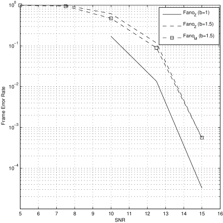
Figure 4: Complexity and Performance of Fano decoder with ZF-DFE and MMSE-DFE based preprocessing for a $30\times 30$ $4-$QAM V-BLAST system

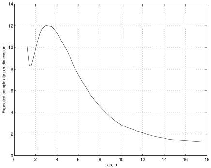
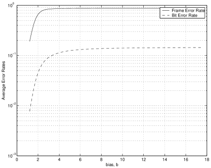
Figure 5: Complexity and Performance of Fano decoder with different bias, for a $20\times 20$ $4-$QAM V-BLAST system with ZF-DFE preprocessing

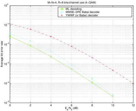
Figure 6: Performance of MMSE-DFE preprocessing with DFE for a $4\times 4$, $4-$QAM V-BLAST system

Thus, one can achieve linear complexity with the stack algorithm by allowing the SNR to increase linearly with the lattice dimension. To validate our theoretical claims, we further report numerical results in selected scenarios. In our simulations, we assume that the channel matrix is square and choose the SE enumeration as the reference sphere decoder for comparison purposes. In all the figures, the subscript $Z$ refers to ZF-DFE left preprocessing and the subscript $M$ denotes MMSE-DFE left preprocessing followed by LLL reduction and V-BLAST greedy ordering for right preprocessing. In Fig. 3, the average complexity per lattice dimension and frame error rate of Fano decoder with $b=1$ and the SE sphere decoder are shown for different values of SNR in a $20\times 20$ $16-$QAM V-BLAST system. Thus, for $m=40$, the Fano decoder can offer a reduction in complexity up-to a factor of 100. Moreover, the performance of the the Fano decoder is seen to be only a fraction of a dB away from that of the SE decoder, which achieves ML performance. We also see that the frame error rate curves for both the Fano decoder and the SE (ML) decoder have the same slope in the high SNR region, as expected from our analysis. Fig. 4 compares the complexity and performance of the Fano decoder with ZF-DFE and MMSE-DFE based preprocessing, respectively, in a $30\times 30$ $4-$QAM V-BLAST system (i.e., $m=60$). From the figures, we see that the MMSE-DFE based preprocessing plays a crucial role in lowering the search complexity of the Fano decoder, despite the apparent increase in search space due to lattice decoding. Fig. 5 reports the dependence of the complexity of the Fano decoder on the value of $b$. The complexity attains a local minimum for some $b^{*}>1$, and for large values of $b$, the complexity of the Fano decoder decreases as $b$ is increased. The error rate, however, increases monotonically with $b$ and approaches that of the MMSE-DFE Babai decoder as $b\rightarrow\infty$. For small dimensions, the performance of the MMSE-DFE based Babai decoder is remarkable. This DFS decoder terminates after finding the first leaf node. Fig. 6 compares the performance of this decoder with the ML performance for a $4\times 4$, $4-$QAM V-BLAST system. We also report the performance of the Yao-Wornell and Windpassinger-Fischer (YWWF) decoder which has the same complexity as the MMSE-DFE Babai decoder [49, 46]. It is shown that the performance of the proposed decoder is within a fraction of a dB from that of ML decoder, whereas the algorithm in [49, 46] exhibits a loss of more than $3$ dB.

5.2 Coded MIMO Systems

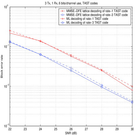
Figure 7: Performance of TAST codes under MMSE-DFE lattice decoding and ML detection with $M=3$ and $N=1$.

In this section, we consider two classes of space-time codes. The first class is the linear dispersion (LD) codes which are obtained by applying a linear transformation (over ${\mathbb{C}}$) to a vector of PAM symbols. For convenience, we follow the set-up of Dayal and Varanasi [16] where two variants of the threaded algebraic space-time (TAST) constellations [19] are used in a $3\times 1$ MIMO channel. This setup also allows for demonstrating the efficiency of the MMSE-DFE frontend in solving under-determined systems. In [16], the rate-$1$ TAST constellation uses $64$-QAM inputs at a rate of one symbol per channel use. The rate-$3$ TAST constellation, on the other hand, uses $4$-QAM inputs to obtain the same throughput as the rate-$1$ constellation. As observed in [16], one obtains a sizable performance gain when using rate-$3$ TAST constellation under ML decoding. The main disadvantage, however, of the rate-3 code is that it corresponds to an under-determined system with $6$ excess unknowns which significantly complicates the decoding problem. Fig. 7 shows that the performance of the proposed MMSE-DFE lattice decoder is less than $0.1$ dB away from the ML decoder for both cases. In order to quantify the complexity reduction offered by our approach, compared with the generalized sphere decoder (GSD) used in [16], we measure the average complexity increase with the excess dimensions. If we define

$$\gamma{\,\,\stackrel{{\scriptstyle\scriptscriptstyle\bigtriangleup}}{{=}}\,\,}\frac{\mbox{Average complexity of decoding rate-$3$ constellation}}{\mbox{Average complexity of decoding rate-$1$ constellation}},$$ (21)

then a straightforward implementation of the GSD, as outlined in [11] for example, would result in $\gamma={\cal O}\left(4^{6}\right)$. In fact, even with the modification proposed in [16], Dayal and Varanasi could only bring this number down to $\gamma=460$ at an SNR of $30$ dB. In Table 1, we report $\gamma$ for the proposed algorithm at different SNRs, where one can see the significant reduction in complexity (i.e., from $460$ to $12$ at an SNR of $30$ dB). Based on experimental observations, we also expect this gain in complexity reduction to increase with the excess dimension $m-n$.

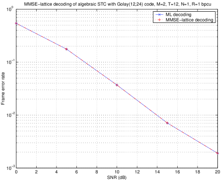
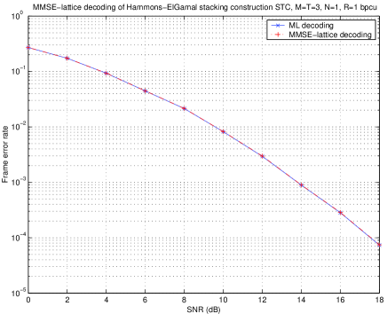
Figure 8: Performance of MMSE-DFE lattice decoding and ML decoding for algebraic space-time codes

The second space-time coding class is the algebraic codes proposed in [31, 41, 40]. This approach constructs linear codes, over the appropriate finite domain, and then the encoded symbols are mapped into QAM constellations. The QAM symbols are then parsed and appropriately distributed across the transmit antennas to obtain full diversity. It has been shown that the complexity of ML decoding of this class of codes grows exponentially with the number of transmit antennas and data rates. Here, we show that the proposed tree search framework allows for an efficient solution to this problem. Figure 8 shows the performance of MMSE-DFE lattice decoding for two such constructions of space-time codes i.e., Golay space-time code for two transmit antennas and the companion matrix code for three transmit antennas [31]. In both case, the performance of the MMSE-DFE lattice decoder is seen to be essentially same as the ML performance. In the proposed decoder, we use the lattice $\Lambda$ obtained from underlying algebraic code through construction A. The ML performance, obtained via exhaustive search in Figure 8, is not feasible for higher dimensions due to exponential complexity in the number of dimensions.

5.3 Coded Transmission over ISI Channels

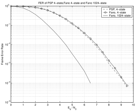
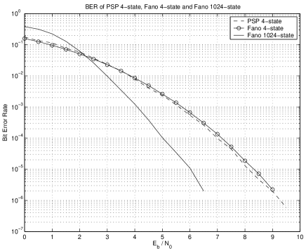
Figure 9: Frame and Bit Error Rate curves for the Fano and PSP algorithms for convolutional codes over an ISI channel

In this section, we compare the performance of the MMSE-Fano decoder with the Per-Survivor-Processing (PSP) algorithm for convolutionally coded transmission over ISI channels. Our MMSE-Fano decoder uses the construction A lattice obtained from the convolutional code. For this scenario, it is known that PSP achieves near-ML frame error rate performance [7]. Figure 9 compares the Frame and Bit Error Rates for a $4-$state, rate $1/2$ convolutional code with generator polynomials given by $(5,7)$ and code length $200$, over a $5-$tap ISI channel. The channel impulse response was chosen as $(0.848,-0.424,0.2545,-0.1696,0.0848)$. The Fano decoder with $b=1$ and stepsize $1$ is seen to achieve essentially the same performance as the PSP algorithm for this code, with reasonable search complexity over the entire SNR range. We again note that the loss in lattice decoding as opposed to finite search space is negligible, due to MMSE-DFE preprocessing of the channel prior to the search. Moreover, the complexity of PSP algorithm, although linear in frame length, increases exponentially with the constraint length of the convolutional code used, while that of the Fano decoder is essentially independent of the constraint length. Figure 9 also shows the performance of the Fano decoder for a rate $1/2$, $1024$-state convolutional code with generator polynomials $(4672,7542)$, with the same frame size. Due to the increased constraint length, the performance is significantly better (with almost no increase in complexity). The complexity of PSP algorithm, on the other hand, is significantly higher for this code.

6 Conclusions

A central goal of this paper was to introduce a unified framework for tree search decoding in wireless communication applications. Towards this end, we identified the roles of two different, but inter-related, components of the decoder, namely; 1) Preprocessing and 2) Tree Search. We presented a preprocessing stage composed of MMSE-DFE filtering for left preprocessing and lattice reduction with column ordering for right preprocessing. We argued that this preprocessor allows for ignoring the boundary control in the tree search stage while entailing only a marginal loss in performance. By relaxing the boundary control, we were able to build a generic framework for designing tree search strategies for joint detection and decoding. Within this framework, BeFS emerged as a very efficient solution that offers many valuable advantages. To limit the storage requirement of BeFS, we re-discovered the Fano decoder as our proposed tree search algorithm. Finally, we established the superior performance-complexity tradeoff of the Fano decoder analytically in a V-BLAST configuration and demonstrated its excellent performance and complexity in more general scenarios via simulation results.

Appendix A The Fano Decoder

In this section, we obtain the cost function used in the proposed Fano/Stack decoder from the Fano metric defined for tree codes over general point-to-point channels, and give a brief description of the Fano decoder and its properties.

A.1 Generic Cost Function of the Fano Decoder

For the transmitted sequence $\hat{\mathbf{x}}$, let

$$\mathbf{y}=\mathbf{R}\hat{\mathbf{x}}+\mathbf{w}$$ (22)

be the system model, as in Section 2. In (22), the noise sequence ${\mathbf{w}}$ is composed of i.i.d Gaussian noise components with zero mean and unit variance.

For a general point-to-point channel with continuous output, the Fano metric of the node ${\mathbf{x}}_{1}^{k}$ can be written as [37]

$$\mu(\mathbf{x}_{1}^{k})=\log\left(\frac{Pr(\mathcal{H}(\mathbf{x}_{1}^{k}))p(\mathbf{y}_{1}^{k}|\mathcal{H}(\mathbf{x}_{1}^{k}))}{p(\mathbf{y}_{1}^{k})}\right)$$ (23)

where $\mathcal{H}({\mathbf{x}}_{1}^{k})$ is the hypothesis that ${\mathbf{x}}_{1}^{k}$ form the first $k$ symbols of the transmitted sequence.

For $1\leq k\leq m$, if $Pr(\mathcal{H}(\mathbf{x}_{1}^{k}))$ is uniform over all nodes $\mathbf{x}_{1}^{k}$ that consist of the first $k$ components of any valid codeword in ${\mathcal{C}}$, from (23), the cost function for the Fano decoder for our system model (22) can be simplified as

$$f({\mathbf{x}}_{1}^{k})=-\mu({\mathbf{x}}_{1}^{k})=\log\left(\sum_{\mathbf{x}_{1}^{k}}e^{-\frac{\sum_{j=1}^{k}w_{j}(\mathbf{x}_{1}^{j})}{2}}\right)+\frac{\sum_{j=1}^{k}w_{j}(\mathbf{x}_{1}^{j})}{2}.$$ (24)

Since summation over $\mathbf{x}_{1}^{k}$ in (24) is not feasible, we use the following approximations: first, $\log(\sum a_{i})\approx\log(\max(a_{i}))$, so the sum can be approximated by the largest term. Second, for moderate to high SNRs, the transmitted sequence is actually the closest vector with a high probability, i.e., the largest term corresponds to the transmitted sequence. Thus, (24) can be approximated as

$$\log\left(\sum_{\mathbf{x}_{1}^{k}}e^{-\frac{\sum_{j=1}^{k}w_{j}(\mathbf{x}_{1}^{j})}{2}}\right)\approx-\frac{|\mathbf{w}_{1}^{k}|^{2}}{2}.$$ (25)

After averaging (25) over noise samples and scaling, we have,

$$f({\mathbf{x}}_{1}^{k})=\sum_{j=1}^{k}w_{j}({\mathbf{x}}_{1}^{j})-k$$

In general, the cost function for the Fano/Stack decoder can be written in terms of the parameter $b$, the bias, as

$$f({\mathbf{x}}_{1}^{k})=\sum_{j=1}^{k}w_{j}({\mathbf{x}}_{1}^{j})-bk.$$

A.2 The Algorithm

The operation of the Fano decoder with no boundary control (lattice decoding) follows the following steps:

• Step 1: (Initialize) Set $k\leftarrow 0$, $T\leftarrow 0$, $\mathbf{x}\leftarrow x_{0}$.

• Step 2: (Look forward) ${\mathbf{x}}_{1}^{k+1}\leftarrow({\mathbf{x}}_{1}^{k},x_{k+1})$, where $x_{k+1}$ is the $(k+1)^{th}$ component of the best child node of ${\mathbf{x}}_{1}^{k}$.

• Step 3:

  If $f(\mathbf{x}_{1}^{k+1})\leq T$,

  If $k+1=m$ (leaf node), then $\hat{\mathbf{x}}={\mathbf{x}}_{1}^{m}$; exit.

  Else (move forward), $k\leftarrow k+1$.

  If $f(\mathbf{x}_{1}^{k-1})>T-\Delta$,

  while $f(\mathbf{x}_{1}^{k})\leq T-\Delta$, $T\leftarrow T-\Delta$ (tighten threshold).

  Go to step 2.

  Else

  If $(k=0$ or $f(\mathbf{x}_{1}^{k-1})>T)$, $T\leftarrow T+\Delta$ (cannot move back, so relax threshold).

  Go to step 2.

  Else (move back and look forward to the next best node)

  ${\mathbf{x}}_{1}^{k}\leftarrow\{{\mathbf{x}}_{1}^{k-1},x_{k}\}$, where $x_{k}$ is the last component of the next best child node of ${\mathbf{x}}_{1}^{k-1}$.

  $k\leftarrow k-1$.

  Go to Step 3. $\Box$

Note that $T$ (i.e., the threshold) is allowed to take values only in multiples of the step size $\Delta$ (i.e., $0,\pm\Delta,\pm 2\Delta,...$). When a node is visited by the Fano decoder for the first time, the threshold $T$ is tightened to the least possible value while maintaining the validity of the node. If the current node does not have a valid child node, then the decoder moves back to the parent node (if the parent node is valid) and attempts moving forward to the next best node. However, if the parent node is not valid, the threshold is relaxed and attempt is made to move forward again, proceeding in this way until a leaf node is reached.

The determination of best and next best child nodes is simplified in CLPS problem; the child node generation order gen in SE enumeration (section 4.1.2) generates child nodes with cost functions in ascending order, given any node ${\mathbf{x}}_{1}^{k}$.

A.3 Properties of the Fano Decoder

The main properties of the Fano decoder used in our analysis are [37]:

1. A node ${\mathbf{x}}_{1}^{k}$ is generated by the Fano decoder only if its cost function is not greater than the bound $T$.

2. Let correct path be defined as the path corresponding to the transmitted codeword, and let $f_{M}$ be the maximum cost function along the correct path. The bound $T$ is always less than $(f_{M}+\Delta)$, where $\Delta$ is the step-size of the Fano decoder; that is, $\max\{T\}<T_{M}{\,\,\stackrel{{\scriptstyle\scriptscriptstyle\bigtriangleup}}{{=}}\,\,}f_{M}+\Delta$.

All nodes that are generated by the Fano decoder are necessarily those with cost function less than the bound $T$, by Property $(1)$. However, even though the cost function of some node ${\mathbf{x}}_{1}^{k}$ may be smaller than the bound, the node itself might not be visited when bound takes the value $T$. If any of the cost functions along the path $\{{\mathbf{x}}_{1}^{r},r<k\}$ increases above $T$, the node ${\mathbf{x}}_{1}^{r}$ is not generated and thus ${\mathbf{x}}_{1}^{k}$ is not visited. Hence, this is not a sufficient condition for a node to be generated.

Moreover, in Property $(2)$, the bound $T$ is always lesser than $(f^{\prime}_{M}+\Delta)$, where $f^{\prime}_{M}$ is the maximum cost function along any path of length $m$. A tight bound is obtained only when the maximum cost function corresponding to the path with the least $f^{\prime}_{M}$ is chosen. However, $f_{M}$ along the transmitted path is usually easier to characterize statistically than $f^{\prime}_{M}$.

Appendix B Properties of the Stack Decoder

For any node ${\bf x}_{1}^{k}$ in the tree, let $h({\bf x}_{1}^{k}){\,\,\stackrel{{\scriptstyle\scriptscriptstyle\bigtriangleup}}{{=}}\,\,}\sum_{i=1}^{k}w_{i}({\bf x}_{1}^{k})-bk$. For the stack algorithm, the cost function of any node in ACTIVE at any instant defined as follows: If ${\bf x}_{1}^{k}$ is a leaf node, then $f({\bf x}_{1}^{k})=-\infty$. Otherwise, we let ${\bf x}_{1,g}^{k+1}$ be the best child node of ${\bf x}_{1}^{k}$ not generated yet, and define $f({\bf x}_{1}^{k})=h({\bf x}_{1,g}^{k})$. We note that $h$ of any node, once generated, remains constant throughout the algorithm, and $f$ of any node is non-decreasing as the algorithm progresses.

Proposition 1

Let $\bar{{\bf x}}_{1}^{m}=(\bar{x}_{1},...\bar{x}_{m})$ be the path chosen by the stack algorithm, and ${\bf x}_{1}^{m}=(x_{1},...,x_{m})$ be any path in the tree. Then,

$$\max_{1\leq j\leq m}h(\bar{{\bf x}}_{1}^{j})\leq\max_{1\leq j\leq m}h({\bf x}_{1}^{j})$$ (26)

Proof :   On the contrary, assume there exists a path $(\bar{x}_{1},\bar{x}_{2},...,\bar{x}_{d},\breve{x}_{d+1},...,\breve{x}_{m})$ that does not satisfy (26). Here, the path is assumed to share the same nodes with the chosen path until level $d$, and diverges from the chosen path from level $d+1$ onwards. Since this path does not satisfy (26),

$$\max_{d+1\leq j\leq m}h(\bar{{\bf x}}_{1}^{j})>\max_{d+1\leq j\leq m}h(\breve{{\bf x}}_{1}^{j})$$ (27)

Let $\bar{{\bf x}}_{1}^{k}$, $k>d$, be the node for which $\max_{d+1\leq j\leq m}h(\bar{{\bf x}}_{1}^{j})$ occurs. Then, we have,

$$h(\bar{{\bf x}}_{1}^{k})>h(\breve{{\bf x}}_{1}^{j}),\quad d<j\leq m$$ (28)

Since $\bar{{\bf x}}_{1}^{m}$ is the chosen path, the node $\bar{{\bf x}}_{1}^{k}$ is generated at some instant before the search terminates. Just before $\bar{{\bf x}}_{1}^{k}$ is generated, $h(\bar{{\bf x}}_{1}^{k-1})=g(\bar{{\bf x}}_{1}^{k})$, since $\bar{{\bf x}}_{1}^{k}$ is the best child node of $\bar{{\bf x}}_{1}^{k-1}$ not generated yet. Moreover, since $h(\bar{{\bf x}}_{1}^{k})>h(\breve{{\bf x}}_{1}^{d+1})$, the node $\bar{{\bf x}}_{1}^{d}$ with cost function $f(\bar{{\bf x}}_{1}^{d})=h(\breve{{\bf x}}_{1}^{d+1})$ appears at the top of the stack at some instant before $\bar{{\bf x}}_{1}^{k}$ is generated. Therefore, $\breve{{\bf x}}_{1}^{d+1}$ is generated before $\bar{{\bf x}}_{1}^{k}$ is generated. Since the search does not terminate before $\bar{{\bf x}}_{1}^{k}$ is generated, applying the same argument, one sees that all the nodes $\breve{{\bf x}}_{1}^{d+2},...,\breve{{\bf x}}_{1}^{m}$ are generated before $\bar{{\bf x}}_{1}^{k}$ is generated. However, once $\breve{{\bf x}}_{1}^{m}$ is generated by the stack algorithm, the search terminates, with $(\bar{x}_{1},...,\bar{x}_{d},\breve{x}_{d+1},...,\breve{x}_{m})$ as the chosen path. Since $1\leq d\leq m$ can take any value, the inequality in (26) is satisfied by all paths.

Proposition 2

If

$$\max_{1\leq j\leq d}h({\bf x}_{1}^{d})>\max_{1\leq j\leq m}h(\bar{{\bf x}}_{1}^{j}),$$ (29)

then, the node ${\bf x}_{1}^{d}$ is not generated.

Proof :   First, we show that if

$$h({\bf x}_{1}^{d})>\max_{1\leq j\leq m}h(\bar{{\bf x}}_{1}^{j}),$$ (30)

then ${\bf x}_{1}^{d}$ is not generated. Let (30) be true, and assume ${\bf x}_{1}^{d}$ is generated. Then, just before ${\bf x}_{1}^{d}$ is generated, its parent node ${\bf x}_{1}^{d-1}$ is at the top of ACTIVE, with cost function $f({\bf x}_{1}^{d-1})=h({\bf x}_{1}^{d})$. However, since $h({\bf x}_{1}^{d})>h(\bar{{\bf x}}_{1}^{j}),\quad 1\leq j\leq m$, all nodes along the chosen path are generated before ${\bf x}_{1}^{d}$ is generated, and the hence the search terminates before ${\bf x}_{1}^{d}$ is generated. Noting that ${\bf x}_{1}^{d}$ can be generated only if all the nodes ${\bf x}_{1}^{1},...,{\bf x}_{1}^{d-1}$ are generated, and applying the same argument for ${\bf x}_{1}^{d-1},...,{\bf x}_{1}^{1}$, we have (29).

Appendix C Proof of Theorem 2

Let ${\mathcal{A}_{IR}}$ be the set of nodes generated by the IR algorithm, where the bounding function ${\bf t}$ has components given by $t_{k}=bk+\delta$. Let ${\mathcal{A}_{s}}$ be the set of nodes generated by the stack decoder with the bias $b$. The IR algorithm in Theorem 2 can be defined with bounding function given by $\{t_{k}=bk+\delta,\quad 1\leq k\leq m\}$, and the cost function for any node ${\mathbf{x}}_{1}^{k}$ given by $\sum_{i=1}^{k}w_{i}({\mathbf{x}}_{1}^{i})$, or equivalently, with the bounding function $t_{k}=\delta$ and cost function $\left(\sum_{i=1}^{k}w_{i}({\mathbf{x}}_{1}^{i})-bk\right)$. If $\delta$ is the bound of the IR algorithm, then any node ${\mathbf{x}}_{1}^{k}$ is generated by the algorithm if and only if all the conditions $\left\{\sum_{i=1}^{1}w_{i}({\mathbf{x}}_{1}^{i})-b<\delta,\sum_{i=1}^{2}w_{i}({\mathbf{x}}_{1}^{i})-2b<\delta,...,\sum_{i=1}^{k}w_{i}({\mathbf{x}}_{1}^{i})-bk<\delta\right\}$, are satisfied. Therefore,

$$\mathcal{A}_{IR}=\left\{\mathbf{x}_{1}^{k}:\max_{1\leq j\leq k}\left(\sum_{i=1}^{k}w_{i}({\mathbf{x}}_{1}^{i})-bk\right)<\delta\right\}.$$ (31)

Moreover, $\delta$ should be such that at least one sequence ${\mathbf{x}}\in{\cal U}$ is included within the search space. Let $\hat{\mathbf{x}}_{IR}$ be a leaf node such that

$$\hat{\mathbf{x}}_{IR}={\hbox{arg}}\min_{\mathbf{x}\in{\cal U}}\left(\max_{1\leq k\leq m}\left(w_{i}({\mathbf{x}}_{1}^{i})-bk\right)\right).$$ (32)

i.e., $\hat{\mathbf{x}}_{IR}$ has the least value of maximum cost function among all paths of length $m$. If

$$\delta<\max_{1\leq j\leq m}\left(w_{i}(\hat{\mathbf{x}}_{IR,1}^{j})-bk\right),$$

then no ${\mathbf{x}}\in{\cal U}$ lies within the search space, and the search space is empty. If lattice decoding is used, then the minimum in (32) is taken over all $\mathbf{x}\in{\mathbb{Z}}^{m}$. Therefore, $\delta>\max_{1\leq j\leq m}\left(w_{i}(\hat{\mathbf{x}}_{IR,1}^{j})-bk\right)$. From Section B, Prop. 1, the path chosen by the stack algorithm, ${\bf x}_{1}^{m}$ satisfies

$$\left(\max_{1\leq k\leq m}\left(w_{i}(\bar{\mathbf{x}}_{1}^{i})-bk\right)\right)\leq\left(\max_{1\leq k\leq m}\left(w_{i}({\mathbf{x}}_{1}^{i})-bk\right)\right)$$ (33)

where ${\bf x}_{1}^{m}$ is any other path.

From (32) and (33),

$$\left(\max_{1\leq k\leq m}\left(w_{i}(\bar{\mathbf{x}}_{1}^{i})-bk\right)\right)=\left(\max_{1\leq k\leq m}\left(w_{i}(\hat{\mathbf{x}}_{IR,1}^{i})-bk\right)\right)<\delta$$ (34)

From Proposition 2 and (33), ${{\cal A}_{s}}\subseteq{{\cal A}_{IR}}$.

Appendix D Proof of Theorem 3

In this section, we derive an upper bound to the frame error rate for a V-BLAST system with uncoded input (with $Q$-PAM constellation for the components), for the Fano decoder that visits paths in the regular $Q$-PAM signal space. The preprocessing assumed here is QR transformation of ${\mathbf{H}}$.

Let ${\mathcal{E}}_{f}$ be the event that the Fano decoder makes an erroneous detection, conditioned on $T_{M}{\,\,\stackrel{{\scriptstyle\scriptscriptstyle\bigtriangleup}}{{=}}\,\,}f_{M}+\Delta$. Then, $P_{e}=E_{T_{M}}(Pr({\mathcal{E}}_{f}))$ is the frame error rate of the Fano decoder. In this section, we derive an upper bound on $P_{e}$. From property $(2)$ in Section A.3, $T<(f_{M}+\Delta)$, where $\Delta$ is the step size of the Fano decoder. Any sequence ${\mathbf{x}}\neq{\hat{\mathbf{x}}}$ can be decoded as the closest point by the Fano decoder only if its cost function is lesser than $T_{M}$. One has

$$\mathbf{y} = \mathbf{H}\mathbf{x}+\mathbf{z}=\mathbf{Q}\begin{pmatrix}{\bf R}\\ \mathbf{0}\end{pmatrix}\mathbf{x}+\mathbf{z},$$ (35)

and therefore

$${\bf y} \leftarrow \mathbf{Q}^{{}^{T}}{\bf y}=\begin{pmatrix}{\bf R}\\ \mathbf{0}\end{pmatrix}\mathbf{x}+\begin{pmatrix}\mathbf{w}_{r+1}^{n}\\ \mathbf{w}_{1}^{r}\end{pmatrix}$$ (36)

where $r=n-m$ is the excess degrees of freedom in the V-BLAST system. Since the cost function of a leaf node ${\mathbf{x}}_{1}^{m}$ is $\displaystyle{f({\mathbf{x}}_{1}^{m})=\sum_{i=1}^{m}w_{i}({\mathbf{x}}_{1}^{i})-bm=|\mathbf{R}\tilde{\mathbf{x}}+\mathbf{w}_{r+1}^{n}|^{2}}-bm$, $P({\mathcal{E}}_{f})$ can be upper bounded as

$$P(\mathcal{E}_{f}) \leq \sum_{{\mathbf{x}}\in{\cal U},{\mathbf{x}}\neq\hat{\mathbf{x}}}\Pr(\sum_{j=1}^{m}w_{j}(\mathbf{x}_{1}^{j})-bm<T_{M})$$ (37)

$$= \sum_{{\mathbf{x}}\in{\cal U},{\mathbf{x}}\neq\hat{\mathbf{x}}}\Pr(|\mathbf{R}\tilde{\mathbf{x}}+\mathbf{w}_{r+1}^{n}|^{2}<bm+f_{M}+\Delta)$$ (38)

where

$$f_{M}=\max\left\{0,|\mathbf{w}_{r+1}^{r+1}|^{2}-b,|\mathbf{w}_{r+1}^{r+2}|^{2}-2b,\ldots,|\mathbf{w}_{r+1}^{n}|^{2}-mb\right\}$$

is the maximum cost function along the transmitted sequence path. The upper bound in (37) follows from the union bound, and due to the fact that in general, $f({\mathbf{x}}_{1}^{m})<T_{M}$ is only a necessary condition for ${\mathbf{x}}_{1}^{m}$ to be decoded by the Fano decoder.

The bound in (38) can be rewritten as

$$P(\mathcal{E}_{f}) \leq \sum_{{\mathbf{x}}\in{\cal U},{\mathbf{x}}\neq\hat{\mathbf{x}}}\Pr\left(\left|\begin{pmatrix}\mathbf{R}\\ \mathbf{0}\end{pmatrix}\tilde{\mathbf{x}}+\mathbf{w}_{1}^{n}\right|^{2}<bm+f_{M}+\Delta+|\mathbf{w}_{1}^{r}|^{2}\right)$$ (39)

$$= \sum_{{\mathbf{x}}\in{\cal U},{\mathbf{x}}\neq\hat{\mathbf{x}}}\Pr\left(\left|\begin{pmatrix}\mathbf{R}\\ \mathbf{0}\end{pmatrix}\tilde{\mathbf{x}}+\mathbf{w}_{1}^{n}\right|^{2}-|\mathbf{w}_{1}^{n}|^{2}<bm+f_{M}+\Delta-|\mathbf{w}_{r+1}^{n}|^{2}\right)$$ (40)

$$= \sum_{{\mathbf{x}}\in{\cal U},{\mathbf{x}}\neq\hat{\mathbf{x}}}\Pr(|\mathbf{H}\tilde{\mathbf{x}}|^{2}+2(\mathbf{H}\tilde{\mathbf{x}})^{{}^{T}}\mathbf{z}<bm+f_{M}+\Delta-|\mathbf{w}_{r+1}^{n}|^{2})$$ (41)

$$\leq \sum_{{\mathbf{x}}\in{\cal U},{\mathbf{x}}\neq\hat{\mathbf{x}}}\Pr(|\mathbf{H}\tilde{\mathbf{x}}|^{2}+2(\mathbf{H}\tilde{\mathbf{x}})^{{}^{T}}\mathbf{z}<bm+\Delta),$$ (42)

since $f_{M}-|\mathbf{w}_{r+1}^{n}|^{2}=\max\left\{-|\mathbf{w}_{r+1}^{n}|^{2},-|\mathbf{w}_{r+2}^{n}|^{2}-b,...,-mb\right\}\leq 0$. The bound in (42) is now independent of the value of $f_{M}$, and hence represents a bound on the frame error rate. Note that the corresponding expression in (42) for ML decoding is $\Pr(|\mathbf{H}\tilde{\mathbf{x}}|^{2}+2(\mathbf{H}\tilde{\mathbf{x}})^{{}^{T}}\mathbf{z}<0)$. For any ${\mathbf{x}}\in{\cal U}$ and ${\mathbf{x}}\neq\hat{\mathbf{x}}$, let $d^{2}({\hat{\mathbf{x}}},\mathbf{x})=|\mathbf{H}\tilde{\mathbf{x}}|^{2}$ represent the squared Euclidean distance between the lattice points ${\mathbf{H}}{\mathbf{x}}$ and ${\mathbf{H}}\hat{\mathbf{x}}$. Then,

$$\Pr(|{\mathbf{H}}\tilde{\mathbf{x}}+\mathbf{z}|^{2}-|\mathbf{z}|^{2}\leq mb+\Delta)\leq\begin{cases}e^{\left(-\frac{1}{8}{(d^{2}({\hat{\mathbf{x}}},\mathbf{x})-mb-\Delta)^{2}}/{d^{2}({\hat{\mathbf{x}}},\mathbf{x})}\right)},&d^{2}({\hat{\mathbf{x}}},\mathbf{x})>mb+\Delta\\ 1&d^{2}({\hat{\mathbf{x}}},\mathbf{x})\leq mb+\Delta\\ \end{cases}$$ (43)

by Chernoff bound.

For $d^{2}({\hat{\mathbf{x}}},\mathbf{x})>mb+\Delta$, equation (43) can be rewritten as

$$\Pr(|{\mathbf{H}}\tilde{\mathbf{x}}+\mathbf{z}|^{2}-|{\bf z}|^{2}\leq mb+\Delta) \leq e^{-\frac{1}{8}\left(d^{2}(\hat{\mathbf{x}},\mathbf{x})+\frac{(mb+\Delta)^{2}}{d^{2}(\hat{\mathbf{x}},\mathbf{x})}-2(mb+\Delta)\right)}$$ (44)

$$\leq e^{-\frac{1}{8}\left(d^{2}(\hat{\mathbf{x}},\mathbf{x})\right)}e^{(mb+\Delta)/4}$$ (45)

since $e^{-(mb+\Delta)^{2}/(8d^{2}(\hat{\mathbf{x}},\mathbf{x}))}<1$, for $d^{2}(\hat{\mathbf{x}},\mathbf{x})>0$. Let

$$q {\,\,\stackrel{{\scriptstyle\scriptscriptstyle\bigtriangleup}}{{=}}\,\,} \min_{\mathbf{x}_{i},\mathbf{x}_{j}\in{\cal U},i\neq j}(|\mathbf{H}(\mathbf{x}_{i}-\mathbf{x}_{j})|^{2})$$ (46)

and let

$$g(q) {\,\,\stackrel{{\scriptstyle\scriptscriptstyle\bigtriangleup}}{{=}}\,\,} \begin{cases}\sum_{{\mathbf{x}}\in{\cal U},\tilde{\mathbf{x}}\neq{\mathbf{0}}}e^{(mb+\Delta)/4}e^{\left(-q/8\right)}&q>mb+\Delta\\ 1&q<mb+\Delta\\ \end{cases}$$ (47)

Then, from (45) and (43), $P_{e}\leq E_{q}(g(q))$. An upper bound on the probability density function (pdf) of $q$ is given by [44]

$$p(q)<p_{\chi}(q)\sum_{k=1}^{m}\left(\begin{array}[]{c}m\\ k\\ \end{array}\right)\frac{1}{k}$$ (50)

where $p_{\chi}(q)$ is the pdf of a scaled chi-square random variable with $n$ degrees of freedom and mean $\frac{n\rho}{m}$ (i.e., a random variable that is the sum of squares of $n$ i.i.d zero-mean Gaussian variables with variance $\frac{\rho}{m}$). Then, (47) and (50) give

$$P_{e} \leq Q^{m}e^{(mb+\Delta)/4}\int_{mb+\Delta}^{\infty}e^{\left(-q/8\right)}p(q)dq+\int_{0}^{mb+\Delta}p(q)dq$$ (51)

$$= AQ^{m}e^{(mb+\Delta)/4}\int_{mb+\Delta}^{\infty}e^{\left(-q/8\right)}\frac{q^{(n/2-1)}e^{-q/(2\sigma^{2})}}{2^{n/2}\Gamma(\frac{n}{2})\sigma^{n}}dq+A\gamma\left(\frac{mb+\Delta}{2\sigma^{2}},\frac{n}{2}\right)$$ (52)

$$\leq AQ^{m}e^{(mb+\Delta)/4}\int_{0}^{\infty}e^{\left(-q/8\right)}\frac{q^{(n/2-1)}e^{-q/(2\sigma^{2})}}{2^{n/2}\Gamma(\frac{n}{2})\sigma^{n}}dq+A\gamma\left(\frac{mb+\Delta}{2\sigma^{2}},\frac{n}{2}\right)$$ (53)

$$= \frac{AQ^{m}e^{(mb+\Delta)/4}}{\left(1+\frac{\rho}{4m}\right)^{n/2}}+A\gamma\left(\frac{mb+\Delta}{2\sigma^{2}},\frac{n}{2}\right)$$ (54)

where $\sigma^{2}=\frac{\rho}{m}$, $A{\,\,\stackrel{{\scriptstyle\scriptscriptstyle\bigtriangleup}}{{=}}\,\,}\displaystyle\sum_{k=1}^{m}\frac{1}{k}{m\choose k}$ is a constant independent of $q$ or $\rho$, and $\gamma(x,a)$ is the incomplete gamma function. If $b$ is bounded (i.e., $b<{\mathcal{M}}<\infty$) $\forall\rho$, then $e^{(mb/4)}$ is also bounded for all $\rho$ and finite $m$. The error performance of the Fano decoder can now be characterized by the sum of two terms. The dependence of the first error term on $\rho$ is of the form $\rho^{-(n/2)}$ for large values of SNR, and hence has the same diversity as the ML decoder. The second term can also be bounded as

$$\gamma\left(\frac{mb+\Delta}{2\sigma^{2}},\frac{n}{2}\right) \leq \left(1-e^{-(mb+\Delta)/(2\sigma^{2})}\right)^{(n/2)}$$ (55)

$$\leq \left(\frac{mb+\Delta}{2\sigma^{2}}\right)^{(n/2)}$$ (56)

$$= \left(\frac{m(mb+\Delta)}{2\rho}\right)^{(n/2)}$$ (57)

where (55) follows from the inequality $\gamma(x,a)\leq(1-e^{-x})^{a}$ (Appendix E.2), and (56) from $(1-e^{-x})<x$ for $x>0$. The second term also has the dependence $\rho^{-(n/2)}$, and hence the Fano decoder achieves the same diversity as that of the ML decoder for this system.

The above derivation also applies to the Stack algorithm, with minor modifications. Let ${\mathcal{E}}_{s}$ be the event that the stack algorithm makes an erroneous detection, conditioned on the value of $f_{M}$. Then, $P_{e}=E_{f_{M}}(\Pr({\mathcal{E}}_{s}))$ is the word error rate of the stack algorithm. Since any path ${\mathbf{x}}\neq{\hat{\mathbf{x}}}$ is decoded as the closest point by the stack algorithm only if $h({\mathbf{x}})=\sum_{i=1}^{m}w_{i}({{\bf x}}_{1}^{i})-bm$ is not greater than $f_{M}$ (Prop. 1, Section B , $P({\mathcal{E}}_{s})$ can be written as

$$P(\mathcal{E}_{s}) \leq \sum_{{\mathbf{x}}\in{\cal U},{\mathbf{x}}\neq\hat{\mathbf{x}}}\Pr\left\{\sum_{j=1}^{m}w_{j}(\mathbf{x}_{1}^{j})-bm<f_{M}\right\}$$ (58)

$$= \sum_{{\mathbf{x}}\in{\cal U},{\mathbf{x}}\neq\hat{\mathbf{x}}}\Pr\left\{|{\mathbf{H}}\tilde{\mathbf{x}}+\mathbf{z}|^{2}<bm+f_{M}\right\}$$ (59)

From (59) and (38), it is easy to see that the error probability expression for the stack algorithm is the same as that for the Fano decoder, when ${\Delta}=0$. Thus, the stack algorithm too achieves the same diversity as the ML decoder for a V-BLAST system, for any finite value of $b$. $\Box$

Appendix E Proof of Theorem 4

The following are required for the proof.

E.1 Wald’s inequality

Let $S_{0}=0,S_{1},S_{2},...$ be a random walk, with $S_{j}=\sum_{i=1}^{j}X_{i}$, where $X_{i}$s are i.i.d random variables such that $\Pr(X_{i}>0)>0$, $\Pr(X_{i}<0)>0$, and $E(X_{i})<0$. Let $g(\lambda)=E(e^{\lambda X_{i}})$ be the moment generating function of $X_{i}$. Let $\lambda_{0}>0$ be a root of $g(\lambda)=1$. Then, from Wald’s identity [37],

$$\Pr(S_{\max}>u)\leq e^{-\lambda_{0}u}$$ (60)

where $S_{\max}=\max_{j}(S_{j})$.

For the random walk with $X_{i}=w_{i}^{2}-b$, where $w_{i}\sim{\mathcal{N}}(0,1)$, the above conditions are satisfied if $b>1$. The moment generating function for $X_{i}=w_{i}^{2}-b$ is given by

$$g(\lambda)=\frac{e^{-\lambda b}}{\sqrt{1-2\lambda}}.$$ (61)

From (61), $\lambda_{0}>0$ can be found as the positive root of the equation

$$-2\lambda b=\log(1-2\lambda).$$

Notice that since $\log(1-2\lambda)$ decreases from $0$ to $-\infty$ as $\lambda$ increases from $0$ to $\frac{1}{2}$, $\lambda_{0}$ satisfies $\lambda_{0}\in(0,0.5)$. Since $\max_{0\leq j\leq m}S_{j}\leq\max_{j\geq 0}S_{j}$, the bound in (60) is also valid for any stopped random walk.

E.2 Upper bounds on $\gamma(\beta,k)$

For a scaled chi-square random variable $X$ with $k$ degrees of freedom and mean $k\sigma^{2}$,

$$\Pr(X\leq\beta)=\gamma\left(\frac{\beta}{2\sigma^{2}},\frac{k}{2}\right)$$

where $\gamma$ is known as the incomplete gamma function. From Chernoff bound, we have

$$\gamma\left(\frac{\beta}{2\sigma^{2}},\frac{k}{2}\right)=\Pr(-X\geq-\beta)\leq\begin{cases}\left(\frac{\beta}{\sigma^{2}k}\right)^{k/2}e^{(\frac{k}{2}-\frac{\beta}{2\sigma^{2}})}&\frac{\beta}{2\sigma^{2}}<\frac{k}{2}\\ 1&\frac{\beta}{2\sigma^{2}}\geq\frac{k}{2}\end{cases}$$ (62)

A simpler, though looser, upper bound is given in [28]:

$$\gamma(x,a)\leq(1-e^{-x})^{a}$$ (63)

E.3 Proof

Let ${\mathbf{x}}_{1}^{k}$ be any path in the tree, and $\displaystyle{h({\mathbf{x}}_{1}^{k})=\sum_{i=1}^{k}w_{i}({\mathbf{x}}_{1}^{i})-bk}$, as in Section B. Let $f_{M}=\max_{1\leq i\leq m}h(\hat{{\bf x}}_{1}^{i})$ be the maximum cost function along the transmitted path. From Section B, Prop. 1, $f_{M}$ is not lesser than the maximum of the cost functions along the path chosen by the stack decoder. From Prop. 2, it is easy to see that any node ${\mathbf{x}}_{1}^{k}$ is generated, only if the maximum of the cost functions along the path ${\mathbf{x}}_{1}^{k}$ does not increase above $f_{M}$.

Let ${\mathcal{A}}_{s,b}$ be the set of generated nodes. In the proof, we upper bound the number of all the paths visited by the algorithm that are different from the correct path, and then we add the complexity of finding the correct path (i.e., $m$). Then, ${\mathcal{A}}_{s,b}$ is a subset of the set of nodes that satisfy $f({\mathbf{x}}_{1}^{k})<f_{M}$. Let ${\bf R}_{k,k}$ be the lower $k\times k$ part of the ${\bf R}$ matrix, i.e.,

$${\bf R}_{k,k}=\left(\begin{array}[]{ccc}r_{k,k}&\ldots&r_{k,1}\\ &\ddots&\vdots\\ \mathbf{0}&&r_{1,1}\end{array}\right)$$

Then, we have,

$$P({\mathbf{x}}_{1}^{k}\in{\mathcal{A}}_{s,b}) \leq P(|{\mathbf{R}}_{k,k}\tilde{\mathbf{x}}_{1}^{k}+{\mathbf{w}}_{r+1}^{r+k}|^{2}-bk<f_{M})$$ (64)

$$= P\left(\left|\begin{pmatrix}{\mathbf{R}}_{k,k}\\ \mathbf{0}\end{pmatrix}\tilde{\mathbf{x}}_{1}^{k}+{\mathbf{w}}_{1}^{r+k}\right|^{2}-bk<f_{M}+|\mathbf{w}_{1}^{r}|^{2}\right)$$ (65)

$$= P\left(\left|\begin{pmatrix}{\mathbf{R}}_{k,k}\\ \mathbf{0}\end{pmatrix}\tilde{\mathbf{x}}_{1}^{k}\right|^{2}+|{\mathbf{w}}_{1}^{r+k}|^{2}+2({\mathbf{w}}_{1}^{r+k})^{{}^{T}}\begin{pmatrix}{\mathbf{R}}_{k,k}\\ \mathbf{0}\end{pmatrix}\tilde{\mathbf{x}}_{1}^{k}-bk<f_{M}+|\mathbf{w}_{1}^{r}|^{2}\right)$$ (66)

where $r=n-m$ is the excess degrees of freedom in the V-BLAST system. From [34], for each $k\leq m$, one can find an $(r+k)\times k$ matrix $\bar{\mathbf{H}}_{r+k,k}$ that has the same distribution as the lower $(r+k)\times k$ part of $\mathbf{H}$, and an $(r+k)\times(r+k)$ unitary matrix $\hbox{\boldmath$\Theta$}^{(r+k)}$ whose distribution is independent of ${\bf R}_{k,k}$, such that $\bar{\mathbf{H}}_{r+k,k}=\mathbf{\Theta}^{(r+k)}\begin{pmatrix}{\bf R}_{k,k}\\ \mathbf{0}\end{pmatrix}$.

Let $\bar{\mathbf{z}}_{1}^{r+k}=\mathbf{\Theta}^{(r+k)}\mathbf{w}_{1}^{r+k}$. The bound in (66) can now be rewritten as

$$P({\mathbf{x}}_{1}^{k}\in{\mathcal{A}}_{s,b}) \leq P(|\bar{\mathbf{H}}_{r+k,k}\tilde{\mathbf{x}}_{1}^{k}|^{2}+2(\bar{\mathbf{z}}_{1}^{r+k})^{{}^{T}}\bar{\mathbf{H}}_{r+k,k}\tilde{\mathbf{x}}_{1}^{k}<f_{M}+bk-|\mathbf{w}_{r+1}^{r+k}|^{2})$$ (67)

In (67), $f_{M}+bk-|\mathbf{w}_{r+1}^{r+k}|^{2}$ can be bounded as

$$f_{M}+bk-|{\mathbf{w}}_{r+1}^{r+k}|^{2} = \max\{bk-|{\mathbf{w}}_{r+1}^{r+k}|^{2},b(k-1)-|{\mathbf{w}}_{r+2}^{r+k}|^{2},\ldots,f^{\prime}_{M}\}$$ (68)

$$\leq \max\{bk,f^{\prime}_{M}\}$$ (69)

where $f^{\prime}_{M}=\max\left\{0,|{\mathbf{w}}_{r+k+1}^{r+k+1}|^{2}-b,\ldots,|{\mathbf{w}}_{r+k+1}^{n}|^{2}-b(m-k)\right\}$. Let $\beta=\max\{bk,f^{\prime}_{M}\}$. (67) can now be rewritten as

$$P({\mathbf{x}}_{1}^{k}\in{\mathcal{A}}_{s,b})\leq P(|\bar{\mathbf{H}}_{r+k,k}\tilde{\mathbf{x}}_{1}^{k}|^{2}+2(\bar{\mathbf{z}}_{1}^{r+k})^{{}^{T}}\bar{\mathbf{H}}_{r+k,k}\tilde{\mathbf{x}}_{1}^{k}<\beta)$$ (70)

Using Chernoff bound, (70) can be written as

$$P({\mathbf{x}}_{1}^{k}\in{\mathcal{B}}_{s,b}|q_{k},\beta)\leq\begin{cases}e^{-(q_{k}-\beta)^{2}/(8q_{k})},&q_{k}>\beta\\ 1,&q_{k}<\beta\\ \end{cases}$$ (71)

where $q_{k}=|\bar{\mathbf{H}}_{r+k,k}\tilde{\mathbf{x}}_{1}^{k}|^{2}$. Let $\eta=\frac{\rho}{m}$. Then, in (71), $\frac{1}{\eta|\tilde{\mathbf{x}}_{1}^{k}|^{2}}{q_{k}}$ is a chi-square random variable with $(r+k)$ degrees of freedom. Since the three random variables, $\bar{\mathbf{H}}_{r+k,k}\tilde{\mathbf{x}}_{1}^{k}$, ${\mathbf{z}}_{1}^{k}$ and $\beta$ are independent, averaging over $q_{k}$ and $\beta$ gives

$$P({\mathbf{x}}_{1}^{k}\in{\mathcal{A}}_{s,b}) \leq E_{\beta}\left(\int_{0}^{\beta}f_{q_{k}}(q_{k})dq_{k}+\int_{\beta}^{\infty}e^{-(q_{k}-\beta)^{2}/(8q_{k})}f_{q_{k}}(q_{k})dq_{k}\right)$$ (72)

$$\leq P(\beta=bk)\left(\int_{0}^{bk}f_{q_{k}}(q_{k})dq_{k}+\int_{bk}^{\infty}e^{-(q_{k}-bk)^{2}/(8q_{k})}f_{q_{k}}(q_{k})dq_{k}\right)+P(\beta>bk)$$ (73)

In (73), $P(\beta>bk)=P(f^{\prime}_{M}>bk)\leq e^{-bk\lambda_{0}}$ for $b>1$ (see Section E.1). Note that one requires $b>1$ because the distribution of the maximum of the cost functions along the transmitted path will depend on $m$ otherwise. The bound in (73) amounts to counting all the nodes ${\bf x}_{1}^{k}$ in the search space when $\beta>bk$. Since $P(\beta>bk)$ decreases sufficiently fast as $k$ increases, this upper bound is still tight for our purposes. Now, (73) can be further simplified as,

$$P({\mathbf{x}}_{1}^{k}\in{\mathcal{A}}_{s,b}) \leq \int_{0}^{bk}f_{q_{k}}(q_{k})dq_{k}+\int_{bk}^{\infty}e^{-(q_{k}-bk)^{2}/(8q_{k})}f_{q_{k}}(q_{k})dq_{k}+e^{-bk\lambda_{0}}$$ (74)

$$\leq \int_{0}^{bk}f_{q_{k}}(q_{k})dq_{k}+\int_{0}^{\infty}e^{-(q_{k}-bk)^{2}/(8q_{k})}f_{q_{k}}(q_{k})dq_{k}+e^{-bk\lambda_{0}}$$ (75)

$$\leq \gamma\left(\frac{bk}{2\eta|\tilde{\mathbf{x}}_{1}^{k}|^{2}},\frac{r+k}{2}\right)+e^{bk/4}\int_{0}^{\infty}e^{-q_{k}/8}f_{q_{k}}(q_{k})dq_{k}+e^{-bk\lambda_{0}}$$ (76)

$$\leq \gamma\left(\frac{bk}{2\eta},\frac{r+k}{2}\right)+\frac{e^{bk/4}}{\left(1+\frac{\eta}{4}\right)^{(r+k)/2}}+e^{-bk\lambda_{0}}$$ (77)

with $\gamma(\cdot,\cdot)$ as the incomplete gamma function. Assuming $r\geq 0$, (77) can be bounded as

$$P({\mathbf{x}}_{1}^{k}\in{\mathcal{A}}_{s,b}) \leq \left(\frac{b}{\eta}e^{1-\frac{b}{\eta}}\right)^{\frac{k}{2}}+\left(\frac{e^{b/2}}{(1+\frac{\eta}{4})}\right)^{\frac{k}{2}}+e^{-bk\lambda_{0}}$$ (78)

for $\eta>b$. The inequality in (78) follows from an upper bound on the incomplete gamma function (see Section E.2). For a node ${\mathbf{x}}_{1}^{k}$, let $G({\mathbf{x}}_{1}^{k})=1$ if the node is generated and $0$ otherwise. Then, the expected number of nodes generated by the algorithm (i.e., complexity) is $\displaystyle{\sum_{k=1}^{m}\sum_{{\mathbf{x}}_{1}^{k}}E[G({\mathbf{x}}_{1}^{k})]}$, where the expectation is over all channel realizations. Let $C_{m}$ be the expected complexity per dimension. Then, assuming a bounded $r$, $C_{m}$ is written as

$$mC_{m}\leq m+\sum_{k=1}^{m}\sum_{{\mathbf{x}}_{1}^{k}}\left(\left(\frac{b}{\eta}e^{1-\frac{b}{\eta}}\right)^{\frac{k}{2}}+\left(\frac{e^{b/2}}{(1+\frac{\eta}{4})}\right)^{\frac{k}{2}}+e^{-bk\lambda_{0}}\right).$$ (79)

The complexity per dimension, $C_{m}$, can now be upper bounded as

$$C_{m} \leq 1+\frac{1}{m}\sum_{k=1}^{m}\sum_{{\mathbf{x}}_{1}^{k}}\left(\left(\frac{b}{\eta}e^{1-\frac{b}{\eta}}\right)^{\frac{k}{2}}+\left(\frac{e^{b/2}}{(1+\frac{\eta}{4})}\right)^{\frac{k}{2}}+e^{-bk\lambda_{0}}\right)$$ (80)

$$\leq 1+\frac{1}{m}\sum_{k=1}^{m}Q^{k}\left(\left(\frac{b}{\eta}e^{1-\frac{b}{\eta}}\right)^{\frac{k}{2}}+\left(\frac{e^{b/2}}{(1+\frac{\eta}{4})}\right)^{\frac{k}{2}}+e^{-bk\lambda_{0}}\right)$$ (81)

$$\leq 1+\frac{1}{m}\left(\frac{1}{1-Q^{2}\frac{b}{\eta}e^{1-\frac{b}{\eta}}}+\frac{1}{1-Q^{2}\frac{e^{b/2}}{(1+\frac{\eta}{4})}}+\frac{1}{1-Qe^{-b\lambda_{0}}}\right),$$ (82)

when $b$ and $\eta$ are sufficiently large, so that all the three sums converge. The inequality in (81) is true, since the number of nodes at level $k$ is $Q^{k}$. Since the terms inside the parenthesis in (82) are all independent of $m$, the number of nodes visited by the stack algorithm scales at most linearly, when $\eta>\eta_{0}$, where $\eta_{0}$ is the minimum $\frac{\rho}{m}$ ratio required for convergence of the sums in (82). $\Box$

Table 1: Complexity Ratio of the proposed algorithm for Rate-$3$ TAST constellation over Rate-$1$ TAST constellation in a $3\times 1$ MIMO System

$\begin{array}[]{|c||c|c|c|c|c|}\hline\cr&&&&&\\ \mbox{SNR (dB)}&22&24&26&28&30\\ \hline\cr\gamma&41&31&23&16&12\\ \hline\cr\end{array}$

Figure 1: Tree representation of the paths searched by sequential decoding algorithms in the case $m=4$.

References

- [1] E. Agrell, T. Eriksson, A. Vardy, and K. Zeger. Closest point search in lattices. IEEE Transactions on Information Theory, 48(8):2201–2214, August 2002.
- [2] J. B. Anderson and S. Mohan. Sequential coding algorithms: A survey and cost analysis. IEEE Trans. Comm., 32:169–176, Feb. 1984.
- [3] L. Babai. On lovasz lattice reduction and the nearest lattice point problem. Combinatorica, 6(1):1–13, 1986.
- [4] S. Baro, J. Hagenauer, and M. Witzke. Iterative detection of MIMO transmission using a list-sequential (LISS) detector. In Proc. IEEE Int. Conf. Communications, pages 2653–2657, May 2003.
- [5] J.-C. Belfiore, G. Rekaya, and E. Viterbo. The golden code: A full-rate space-time code with nonvanishing determinants. IEEE Transactions on Information Theory, 51(4):1432 – 1436, Apr. 2005.
- [6] J. Benesty, Y. A. Huang, and J. Chen. A fast recursive algorithm for optimum sequential signal detection in a blast system. IEEE Trans. Signal Processing, 51:1722–1731, July 2003.
- [7] G. Caire and G. Colavolpe. On low complexity space-time coding for quasi-static channels. IEEE Trans. Info. Theory, 49(6):1400–1416, June 2003.
- [8] J. M. Cioffi, G. P. Dudevoir, M. V. Eyuboglu, and G. D. Forney Jr. MMSE decision-feedback equalizers and coding. I. equalization results. IEEE Transactions on Communications, 43(10):2582 – 2594, Oct. 1995.
- [9] H. Cohen. A Course in Computational Algebraic Number Theory. Springer-Verlag, 1995.
- [10] J. H. Conway and N. J. A. Sloane. Sphere Packings, Lattices, and Groups, 3rd ed. Springer-Verlag New York, 1999.
- [11] M. O. Damen, K. Abed-Meraim, and J.-C. Belfiore. Generalized sphere decoder for asymmetrical space-time communication architecture. Electron. Lett, 36:166, Jan. 2000.
- [12] M. O. Damen, A. Chkeif, and J.-C. Belfiore. Lattice codes decoder for space-time codes. IEEE Commun. Lett., 4:161–163, May 2000.
- [13] M. O. Damen, H. El Gamal, and N. C. Beaulieu. Linear threaded algebraic space-time constellations. IEEE Transactions on Information Theory, 49(10):2372–2388, Oct. 2003.
- [14] M. O. Damen, H. El Gamal, and G. Caire. On maximum-likelihood detection and the search for the closest lattice point. IEEE Transactions on Information Theory, 49:2389–2401, Oct. 2003.
- [15] M. O. Damen, H. El Gamal, and G. Caire. MMSE-GDFE lattice decoding for under-determined linear channels. In 38th Annual Conf. on Inform. Sciences and Systems, March 2004.
- [16] P. Dayal and M. K. Varanasi. A fast generalized sphere decoder for optimum decoding of under-determined MIMO systems. In Proc. 41th Annual Allerton Conf. on Comm. Control, and Comput., Monticello, IL, Oct. 2003.
- [17] A. Duel-Hallen and C. Heegard. Delayed decision-feedback sequence estimation. IEEE Transactions on Communications, 37:428–436, May 1989.
- [18] H. El Gamal, G. Caire, and M. O. Damen. Lattice coding and decoding achieve the optimal diversity-multiplexing tradeoff of MIMO channels. IEEE Transactions on Information Theory, 50(6):968–985, June 2004.
- [19] H. El Gamal and M. O. Damen. Universal space-time coding. IEEE Transactions on Information Theory, 49:1097–1119, May 2003.
- [20] U. Erez, S. Litsyn, and R. Zamir. Lattices which are good for (almost) everything. In Proc. IEEE Information Theory Workshop, 2003, pages 271–274, Apr. 2003.
- [21] U. Erez and R. Zamir. Achieving on the AWGN channel with lattice encoding and decoding. IEEE Transactions on Information Theory, 50(10):2293 – 2314, Oct. 2004.
- [22] R. M. Fano. A heuristic discussion of probabilistic decoding. IEEE transactions on Information Theory, 9(2):64–74, Apr. 1963.
- [23] U. Fincke and M. Pohst. Improved methods for calculating vectors of short length in a lattice, including a complexity analysis. Math. of Comput., 44:463–471, Apr. 1985.
- [24] G. D. Forney Jr. Coset codes. I. introduction and geometrical classification. IEEE Transactions on Information Theory, 34(5):1123 – 1151, Sept. 1988.
- [25] G. D. Forney Jr. Coset codes. II. binary lattices and related codes. IEEE Transactions on Information Theory, 34(5):1152 – 1187, Sept. 1988.
- [26] G. Foschini. Layered space-time architecture for wireless communication in a fading environment using multi-element antennas. Bell labs Tech J., 1(2):41–59, 1996.
- [27] J. Foschini, G. Golden, R. Valenzuela, and P. Wolniansky. Simplified processing for high spectral efficiency wireless communication employing multi-element arrays. IEEE J. Select. Areas Commun., 17(11):1841–1852, Nov. 1999.
- [28] W. Gautschi. The incomplete gamma functions since Tricomi. In Tricomi’s ideas and contemporary applied mathematics, Atti Convegni Lincei, Rome, pages 203–237, 1998.
- [29] J. Geist. Search properties of some sequential decoding algorithms. IEEE Transactions on Information Theory, 19(4):519–526, July 1973.
- [30] R. Gowaikar and B. Hassibi. Efficient statistical pruning for maximum likelihood decoding. In Proceedings of the 2003 IEEE International Conference on Acoustics, Speech and Signal Processing, pages V–49–52, April 2003.
- [31] A. R. Hammons Jr and H. El Gamal. On the theory of space-time codes for PSK modulation. IEEE Transactions on Information Theory, 46(2):524 – 542, March 2000.
- [32] B. Hassibi. An efficient square-root algorithm for BLAST. In Proceedings of the 2000 IEEE International Conference on Acoustics, Speech and Signal Processing, pages II737 – II740, June 2000.
- [33] B. Hassibi and B. Hochwald. High-rate codes that are linear in space and time. IEEE Transactions on Information Theory, 48(7):1804 – 1824, July 2002.
- [34] B. Hassibi and H. Vikalo. On sphere decoding algorithm. I. expected complexity. Submitted to IEEE Transactions on Signal Processing.
- [35] B. Hochwald and S. ten Brink. Achieving near-capacity on a multiple-antenna channel. IEEE Transactions on Communications, 51(3):389 – 399, March 2003.
- [36] J. Jalden and B. Ottersten. On the complexity of sphere decoding in digital communications. IEEE Trans. Signal Proc., 53(4):1474 – 1484, Apr. 2005.
- [37] R. Johannesson and K. Zigangirov. Fundamentals of convolutional coding. Wiley-IEEE press, 1999.
- [38] M. Kokkonen and K. Kalliojarvi. Soft-decision decoding of binary linear codes using the -algorithm. In Proc. IEEE th intl. symp. on PIMRC, pages 1181–1185, Sep. 1997.
- [39] A. K. Lenstra, A. W. Lenstra Jr., and L. Lovasz. On factoring polynomials with rational coefficients. Math. Annalen., 261:515–534, 1982.
- [40] Y. Liu, M. Fitz, and O. Takeshita. A rank criterion for qam space-time codes. IEEE Trans. Info. Theory, 48(12):3062–3079, Dec. 2002.
- [41] H.-F. Lu and P. Kumar. A unified construction of space-time codes with optimal rate-diversity tradeoff. IEEE Transactions on Information Theory, 51(5):1709 – 1730, May 2005.
- [42] C. P. Schnorr and M. Euchner. Lattice basis reduction: Improved practical algorithms and solving subset sum problems. Math. Programming, 66:181–191, 1994.
- [43] B. A. Sethuraman, B. S. Rajan, and V. Shashidhar. Full-diversity, high-rate space-time block codes from division algebras. IEEE Transactions on Information Theory, 49(10):2596 – 2616, Oct. 2003.
- [44] R. van Nee, A. van Zelst, and G. Awater. Maximum likelihood decoding in a space division multiplexing system. In Vehicular Technology Conference, pages 6–10, May 2000.
- [45] E. Viterbo and J. Boutros. A universal lattice code decoder for fading channels. IEEE Transactions on Information Theory, 45(5):1639–1642, 1999.
- [46] C. Windpassinger and R. Fischer. Low-complexity near-maximum-likelihood detection and precoding for MIMO systems using lattice reduction. In Proc. IEEE Inform. Theory Workshop, Paris, France,, Mar. 2003.
- [47] J. M. Wozencraft and B. Reiffen. Sequential decoding. MIT press and Wiley, 1961.
- [48] W. Xu, Y. Wang, Z. Zhou, and J. Wang;. A computationally efficient exact ML sphere decoder. In IEEE Global Telecommunications Conference, 2004., pages 2594 – 2598, Nov 2004.
- [49] H. Yao and G. Wornell. Lattice-reduction-aided detectors for MIMO communication systems. In Proc. IEEE Global Conf. on Commun., Taipei, Taiwan, Nov. 2002.