Technical Report IDSIA-13-05  
Asymptotics of Discrete MDL
for Online Prediction
 

Abstract

Minimum Description Length (MDL) is an important principle for induction and prediction, with strong relations to optimal Bayesian learning. This paper deals with learning non-i.i.d. processes by means of two-part MDL, where the underlying model class is countable. We consider the online learning framework, i.e. observations come in one by one, and the predictor is allowed to update his state of mind after each time step. We identify two ways of predicting by MDL for this setup, namely a static and a dynamic one. (A third variant, hybrid MDL, will turn out inferior.) We will prove that under the only assumption that the data is generated by a distribution contained in the model class, the MDL predictions converge to the true values almost surely. This is accomplished by proving finite bounds on the quadratic, the Hellinger, and the Kullback-Leibler loss of the MDL learner, which are however exponentially worse than for Bayesian prediction. We demonstrate that these bounds are sharp, even for model classes containing only Bernoulli distributions. We show how these bounds imply regret bounds for arbitrary loss functions. Our results apply to a wide range of setups, namely sequence prediction, pattern classification, regression, and universal induction in the sense of Algorithmic Information Theory among others.

Keywords

Minimum Description Length, Sequence Prediction, Consistency, Discrete Model Class, Universal Induction, Stabilization, Algorithmic Information Theory, Loss Bounds, Classification, Regression.

1 Introduction

“Always prefer the simplest explanation for your observation,” says Occam’s razor. In Learning and Information Theory, simplicity is often quantified in terms of description length, giving immediate rise to the Minimum Description Length (MDL) principle [WB68, Ris78, Grü98]. Thus MDL can be seen as a strategy against overfitting. An alternative way to think of MDL is Bayesian. The explanations for the observations (the models) are endowed with a prior. Then the model having maximum a posteriori (MAP) probability is also a two-part MDL estimate, where the correspondence between probabilities and description lengths is simply by a negative logarithm.

How does two-part MDL perform for prediction? Some very accurate answers to this question have been already given. If the data is generated by an independently identically distributed (i.i.d.) process, then the MDL estimates are consistent [BC91]. In this case, an important quantity to consider is the index of resolvability, which depends on the complexity of the data generating process. This quantity is a tight bound on the regret in terms of coding (i.e. the excess code length). Moreover, the index of resolvability also bounds the predictive regret, namely the rate of convergence of the predictive distribution to the true one. These results apply to both discrete and continuously parameterized model classes, where in the latter case the MDL estimator must be discretized with an appropriate precision.

Under the relaxed assumption that the data generating process obeys a central limit theorem and some additional conditions, Rissanen [Ris96, BRY98] proves an asymptotic bound on the regret of MDL codes. Here, he also removes the coding redundancy arising if two-part codes are defined in the straightforward way. The resulting bound is very similar to that in [CB90] for Bayes mixture codes and i.i.d. processes, where the i.i.d. assumption may also be relaxed [Hut03b]. Other similar and related results can be found in [GV01, GV04].

In this work, we develop new methods in order to arrive at very general consistency theorems for MDL on countable model classes. Our setup is online sequence prediction, that is, the symbols $x_{1},x_{2},\ldots$ of an infinite sequence are revealed successively by the environment, where our task is to predict the next symbol in each time step. Consistency is established by proving finite cumulative bounds on the differences of the predictive to the true distribution. Differences will be measured in terms of the relative entropy, the quadratic distance, and the Hellinger distance. Most of our results are based on the only assumption that the data generating process is contained in the models class. (The discussion of how strong this assumption is, will be postponed to the last section.) Our results imply regret bounds with arbitrary loss functions. Moreover, they can be directly applied to important general setups such as pattern classification, regression, and universal induction.

As many scientific models (e.g. in physics or biology) are smooth, much statistical work is focussed on continuous model classes. On the other hand, the largest relevant classes from a computational point of view are at most countable. In particular, the field of Algorithmic Information Theory (also known as Kolmogorov Complexity, e.g. [ZL70, LV97, Cal02, Hut04]) studies the class of all lower-semicomputable semimeasures. Then there is a one-to-one correspondence of models and programs on a fixed universal Turing Machine. (Since programs need not halt on each input, models are semimeasures instead of measures, see e.g. [LV97] for details). This model class can be considered the largest one which can be in the limit processed under standard computational restrictions. We will develop all our results for semimeasures, so that they can be applied in this context, which we refer to as universal sequence prediction.

In the universal setup, the Bayes mixture is also termed Solomonoff-Levin prior and has been intensely studied first by Solomonoff [Sol64, Sol78]. Its predictive properties are excellent [Hut01, Hut04]. Precisely one can bound the cumulative loss by the complexity of the data generating process. This is the reference performance we compare MDL to. It turns out that the predictive properties of MDL can be exponentially worse, even in the case that the model class contains only Bernoulli distributions. Another related quantity in the universal setup is one-part MDL, which has been studied in [Hut03c]. We will briefly encounter it in Section 8.4.

The paper is structured as follows. Section 2 establishes basic definitions. In Section 3, we introduce the MDL estimator and show how it can be used for sequence prediction in at least three ways. Sections 4 and 5 are devoted to convergence theorems. In Sections 6 and 7, we study the stabilization properties of the MDL estimator. Section 8 presents more general loss bounds as well as three important applications: pattern classification, regression, and universal induction. Finally, Section 9 contains the conclusions.

2 Prerequisites and Notation

We build on the notation of [LV97] and [Hut04]. Let the alphabet $\mathcal{X}$ be a finite set of symbols. We consider the spaces $\mathcal{X}^{*}$ and $\mathcal{X}^{\infty}$ of finite strings and infinite sequences over $\mathcal{X}$. The initial part of a sequence up to a time $t\in\mathbb{N}$ or $t-1\in\mathbb{N}$ is denoted by $x_{1:t}$ or $x_{<t}$, respectively. The empty string is denoted by $\epsilon$.

A semimeasure is a function $\nu:\mathcal{X}^{*}\to[0,1]$ such that

$$\nu(\epsilon)\leq 1\;\mbox{ and }\;\nu(x)\geq\sum_{a\in\mathcal{X}}\nu(xa)\;\mbox{ for all }\;x\in\mathcal{X}^{*}$$ (1)

holds. If equality holds in both inequalities of (1), then we have a measure. Intuitively, the quantity $\nu(x)$ can be understood as the probability that a data generating process yields a string starting with $x$. Then, for a measure, the probabilities of all joint continuations of $x$ add up to $\nu(x)$, while for a semimeasure, there may be a “probability leak” (1). Recall that we are interested in semimeasures (and not only in measures) because of their correspondence to programs on a fixed universal Turing machine in the universal setup and our inability to decide the halting problem.

Let $\mathcal{C}$ be a countable class of (semi)measures, i.e. $\mathcal{C}=\{\nu_{i}:i\in I\}$ with finite or infinite index set $I\subseteq\mathbb{N}$. A (semi)measure $\tilde{\nu}$ dominates the class $\mathcal{C}$ iff for every $\nu_{i}\in\mathcal{C}$ there is a constant $c_{i}>0$ such that $\nu(x)\geq c_{i}\cdot\nu_{i}(x)$ holds for all $x\in\mathcal{X}^{*}$. A dominant semimeasure $\tilde{\nu}$ need not be contained in $\mathcal{C}$.

Each (semi)measure $\nu\in\mathcal{C}$ is associated with a weight $w_{\nu}>0$, and we require $\sum_{\nu}w_{\nu}\leq 1$. We may interpret the weights as a prior on $\mathcal{C}$. Then it is obvious that the Bayes mixture

$$\xi(x)\equiv\xi_{[\mathcal{C}]}(x):=\sum_{\nu\in\mathcal{C}}w_{\nu}\nu(x)\quad(\mbox{for }x\in\mathcal{X}^{*})$$ (2)

dominates $\mathcal{C}$. Assume that there is some measure $\mu\in\mathcal{C}$, the true distribution, generating sequences $x_{<\infty}\in\mathcal{X}^{\infty}$. Typically $\mu$ is unknown. (Note that we require $\mu$ to be a measure: The data stream always continues, there are no “probability leaks”.) If some initial part $x_{<t}$ of a sequence is given, the probability of observing $x_{t}\in\mathcal{X}$ as a next symbol is

$$\mu(x_{t}|x_{<t})=\frac{\mu(x_{<t}x_{t})}{\mu(x_{<t})}\;\mbox{ if }\;\mu(x_{<t})>0\ \;\mbox{ and }\;\ \mu(x_{t}|x_{<t})=0\;\mbox{ if }\;\mu(x_{<t})=0.$$ (3)

and, for well-definedness, $\mu(x_{t}|x_{<t})=0$ if $\mu(x_{<t})=0$ (this case has probability zero). Note that $\mu(x_{t}|x_{<t})$ can depend on the complete history $x_{<t}$. We may generally define the quantity (3) for any function $\varphi:\mathcal{X}^{*}\to[0,1]$; we call $\varphi(x_{t}|x_{<t}):=\frac{\varphi(x_{1:t})}{\varphi(x_{<t})}$ the $\varphi$-prediction. Clearly, this is not necessarily a probability on $\mathcal{X}$ for general $\varphi$. For a semimeasure $\nu$ in particular, the $\nu$-prediction $\nu(\cdot|x_{<t})$ is a semimeasure on $\mathcal{X}$.

We define the expectation with respect to the true probability $\mu$: Let $n\geq 0$ and $f:\mathcal{X}^{n}\to\mathbb{R}$ be a function, then

$${\mathbf{E}}\ f={\mathbf{E}}\ f(x_{1:n})=\sum_{x_{1:n}\in\mathcal{X}^{n}}\mu(x_{1:n})f(x_{1:n}).$$ (4)

More general, the expectation may be defined as an integral over infinite sequences. But since we won’t need it, we can keep things simple. The following is a central result about prediction with Bayes mixtures in a form independent of Algorithmic Information Theory.

Theorem 1

For any class of (semi)measures $\mathcal{C}$ containing the true distribution $\mu$, which is a measure, we have

$$\sum_{t=1}^{\infty}{\mathbf{E}}\sum_{a\in\mathcal{X}}\Big{(}\mu(a|x_{<t})-\xi(a|x_{<t})\Big{)}^{2}\ \leq\ \ln w_{\mu}^{-1}.$$ (5)

This was found by Solomonoff ([Sol78]) for universal sequence prediction. A proof is also given in [LV97] (only for binary alphabet) or [Hut04] (arbitrary alphabet). It is surprisingly simple once Lemma 6 is known. A few lines analogous to (14) and (15) exploiting the dominance of $\xi$ are sufficient.

One should be aware that the condition $\mu\in\mathcal{C}$ is essential in general, for both Bayes and MDL predictions [GL04]. On the other hand, one can show that if there is an element in $\mathcal{C}$ which is sufficiently close to $\mu$ in an appropriate sense, then still good predictive properties hold [Hut03b].

Note that although $w_{\nu}$ can be interpreted as a prior on the model class, we do not assume any probabilistic structure for $\mathcal{C}$ (e.g. a sampling mechanism). The theorem rather states that the cumulative loss is bounded by a quantity depending on the complexity $\ln w_{\mu}^{-1}$ of the true distribution. The same kind of assertion will be proven for MDL predictions later.

The bound (5) implies that the $\xi$-predictions converge to the $\mu$-predictions almost surely (i.e. with $\mu$-probability one). This is not hard to see, since with the abbreviation $s_{t}=\sum_{a}\big{(}\mu(a|x_{<t})-\xi(a|x_{<t})\big{)}^{2}$ and for each $\varepsilon>0$, we have

$${\mathbf{P}}\Big{(}\exists t\geq n:s_{t}\geq\varepsilon\Big{)} = {\mathbf{P}}\Big{(}\bigcup_{t\geq n}\big{\{}s_{t}\geq\varepsilon\big{\}}\Big{)}$$ (6)

$$\leq \sum_{t\geq n}{\mathbf{P}}\big{(}s_{t}\geq\varepsilon\big{)}\ \leq\ \frac{1}{\varepsilon}\sum_{t=n}^{\infty}{\mathbf{E}}s_{t}\ \stackrel{{\scriptstyle n\to\infty}}{{\longrightarrow}}\ 0.$$

Actually, (5) yields an even stronger assertion, since it characterizes the speed of convergence by the quantity on the right hand side. Precisely, the expected number of times $t$ in which $\xi(a|x_{<t})$ deviates by more than $\varepsilon$ from $\mu(a|x_{<t})$ is finite and bounded by $\ln w_{\mu}^{-1}/\varepsilon^{2}$, and the probability that the number of $\varepsilon$-deviations exceeds $\ln w_{\mu}^{-1}\over\varepsilon^{2}\delta$ is smaller than $\delta$. (However, we cannot conclude a convergence rate of $s_{t}=o(\frac{1}{t})$ from (5), since the quadratic differences generally do not decrease monotonically.)

Since we will encounter this type of convergence (5) frequently in the following, we call it convergence in mean sum (i.m.s):

$$\varphi\stackrel{{\scriptstyle i.m.s.}}{{\longrightarrow}}\mu\quad\Longleftrightarrow\quad\exists\ C>0:\ \sum_{t=1}^{\infty}{\mathbf{E}}\sum_{a\in\mathcal{X}}\Big{(}\mu(a|x_{<t})-\varphi(a|x_{<t})\Big{)}^{2}\!<\infty.$$ (7)

Then Theorem 1 states that the $\xi$ predictions converge to the $\mu$ predictions i.m.s., or “$\xi$ converges to $\mu$ i.m.s.” for short. By (6), convergence i.m.s. implies almost sure convergence (with respect to the true distribution $\mu$). Note that in contrast, convergence in the mean, i.e. ${\mathbf{E}}[\sum_{a}(\mu(a|x_{<t})-\varphi(a|x_{<t}))^{2}]\stackrel{{\scriptstyle t\to\infty}}{{\longrightarrow}}0$, only implies convergence in probability.

Probabilities vs. Description Lengths. By the Kraft inequality, each (semi)measure can be associated with a code length or complexity by means of the negative logarithm, where all (binary) codewords form a prefix-free set. The converse holds as well. We introduce the abbreviation

$$K\!\ \ldots=-{\log_{2}}\ldots,\mbox{ e.g. }K\!\nu(x)=-{\log_{2}}\nu(x)$$ (8)

for a semimeasure $\nu$ and $x\in\mathcal{X}^{*}$ and $K\!\xi(x)=-{\log_{2}}\xi(x)$ for the Bayes mixture $\xi$. It is common to ignore the somewhat irrelevant restriction that code lengths must be integer. In particular, given a class of semimeasures $\mathcal{C}$ together with weights, each weight $w_{\nu}$ corresponds to a description length or complexity

$$K\!w(\nu)=-{\log_{2}}w_{\nu}.$$ (9)

It is often only a matter of notational convenience if description lengths or probabilities are used, but description lengths are generally preferred in Algorithmic Information Theory. Keeping the equivalence in mind, we will develop the general theory in terms of probabilities, but formulate parts of the results in universal sequence prediction rather in terms of complexities.

3 MDL Estimator and Predictions

Assume that $\mathcal{C}$ is a countable class of semimeasures together with weights $(w_{\nu})_{\nu\in\mathcal{C}}$, and $x\in\mathcal{X}^{*}$ is some string. Then the maximizing element $\nu^{x}$, often called MAP (maximum a posteriori) estimator, is defined as

$$\nu^{x}=\nu^{x}_{[\mathcal{C}]}=\arg\max_{\nu\in\mathcal{C}}\{w_{\nu}\nu(x)\}.$$ (10)

In case of a tie, we need not specify the further choice at this point, just pick any of the maximizing elements. But for concreteness, you may think that ties are broken in favor of larger prior weights. The maximum is always attained in (10) since for each $\varepsilon>0$ at most a finite number of elements fulfil $w_{\nu}\nu(x)>\varepsilon$. Observe immediately the correspondence in terms of description lengths rather than probabilities:

$$\nu^{x}=\arg\min_{\nu\in\mathcal{C}}\big{\{}K\!w(\nu)+K\!\nu(x)\big{\}}.$$

Then the minimum description length principle is obvious: $\nu^{x}$ minimizes the joint description length of the model plus the data given the model (see (8) and (9)). As explained before, we stick to the product notation.

For notational simplicity, let $\nu^{*}(x)=\nu^{x}(x)$. The two-part MDL estimator is defined by

$$\varrho(x)=\varrho_{[\mathcal{C}]}(x)=w_{\nu^{x}}\nu^{x}(x)=\max_{\nu\in\mathcal{C}}\{w_{\nu}\nu(x)\}.$$

So $\varrho$ chooses the maximizing element with respect to its argument. We may also use the version $\varrho^{y}(x):=w_{\nu^{y}}\nu^{y}(x)$ for which the choice depends on the superscript instead of the argument. Note that the use of the term “estimator” is non-standard, since $\varrho$ is a product of the estimator $\nu^{*}$ (this use is standard) and its prior weight. There will be no confusion between these two meanings of “estimator” in the following.

For each $x,y\in\mathcal{X}^{*}$,

$$\xi(x)\geq\varrho(x)\geq\varrho^{y}(x)$$ (11)

is immediate. If $\mathcal{C}$ contains only measures, we have $\sum_{a}\varrho(xa)\geq\sum_{a}\varrho^{x}(xa)=\varrho^{x}(x)=\varrho(x)$ for all $x\in\mathcal{X}^{*}$, so $\varrho$ has some “anti-semimeasure” property. If $\mathcal{C}$ contains semimeasures, no semimeasure or anti-semimeasure property can be established for $\varrho$.

We can define MDL predictors according to (3). There are basically two possible ways to use MDL for prediction.

Definition 2

The dynamic MDL predictor is defined as

$$\varrho(a|x)=\frac{\varrho(xa)}{\varrho(x)}=\frac{\varrho^{xa}(xa)}{\varrho^{x}(x)}.$$

That is, we look for a short description of $xa$ and relate it to a short description of $x=x_{<t}$. We call this dynamic since for each possible $a$ we have to find a new MDL estimator. This is the closest correspondence to the Bayes mixture $\xi$-predictor.

Definition 3

The static MDL predictor is given by

$$\varrho^{\mathrm{static}}(a|x)=\varrho^{x}(a|x)=\frac{\varrho^{x}(xa)}{\varrho(x)}=\frac{\varrho^{x}(xa)}{\varrho^{x}(x)}=\frac{\nu^{x}(xa)}{\nu^{x}(x)}.$$

Here obviously only one MDL estimator $\varrho^{x}$ has to be identified. This is usually more efficient in practice.

We will define another MDL predictor, the hybrid one, in Section 6. It can be paraphrased as “do dynamic MDL but drop weights”. We will see that its predictive performance is weaker.

The range of the static MDL predictor is obviously contained in $[0,1]$. For the dynamic MDL predictor, this holds by

$$\varrho^{x}(x)\geq\varrho^{xa}(x)\geq\varrho^{xa}(xa).$$ (12)

Static MDL is omnipresent in machine learning and applications, see also Section 8. In fact, many common prediction algorithms can be abstractly understood as static MDL, or rather as approximations. Namely, if a prediction task is accomplished by building a model such as a neural network with a suitable regularization to prevent “overfitting”, this is just searching an MDL estimator within a certain class of distributions. After that, only this model is used for prediction. Dynamic MDL is applied more rarely due to its larger computational effort. For example, the similarity metric proposed in [LCL⁺03] can be interpreted as (a deterministic variant of) dynamic MDL.

We will need to convert our MDL predictors to measures by means of normalization. If $\varphi:\mathcal{X}^{*}\to[0,1]$ is any function, then

$$\varphi_{\mathrm{norm}}(a|x)\ :=\ \frac{\varphi(a|x)}{\sum_{b\in\mathcal{X}}\varphi(b|x)}\ =\ \frac{\varphi(xa)}{\sum_{b\in\mathcal{X}}\varphi(xb)}$$

is a measure (assume that the denominator is different from zero, which is always true with probability 1 (w.p.1) if $\varphi$ is an MDL predictor). This procedure is known as Solomonoff normalization [Sol78, LV97] and results in

$$\varphi_{\mathrm{norm}}(x_{1:n})=\frac{\varphi(x_{1:n})}{\varphi(\epsilon)}\prod_{t=1}^{n}\frac{\varphi(x_{<t})}{\sum_{a\in\mathcal{X}}\varphi(x_{<t}a)}={\varphi(x_{1:n})\over\varphi(\epsilon)N_{\varphi}(x_{<n})},$$

where

$$N_{\varphi}(x)=\prod_{t=1}^{\ell(x)+1}\frac{\sum_{a\in\mathcal{X}}\varphi(x_{<t}a)}{\varphi(x_{<t})}$$ (13)

is the normalizer.

We conclude this section with a simple example.

Bernoulli and i.i.d. classes. Let $n\in\mathbb{N}$, $\mathcal{X}=\{1,\ldots,n\}$, and

$$\mathcal{C}=\Big{\{}\nu_{\vartheta}(x_{1:t})=\vartheta_{x_{1}}\!\cdot...\!\cdot\vartheta_{x_{t}}:\vartheta\in\Theta\Big{\}}\mbox{\quad with\quad}\Theta=\Big{\{}\vartheta\in([0,1]\cap\mathbb{Q})^{n}:\sum_{i=1}^{n}\vartheta_{i}=1\Big{\}}$$

be the set of all rational probability vectors with any prior $(w_{\vartheta})_{\vartheta\in\Theta}$. Each $\vartheta\in\Theta$ generates sequences $x_{<\infty}$ of independently identically distributed (i.i.d.) random variables such that ${\mathbf{P}}(x_{t}=i)=\vartheta_{i}$ for all $t\geq 1$ and $1\leq i\leq n$. If $x_{1:t}$ is the initial part of a sequence and $\alpha\in\Theta$ is defined by $\alpha_{i}=\frac{1}{t}|\{s\leq t:x_{s}=i\}|$, then it is easy to see that

$$\nu^{x_{1:t}}=\arg\min_{\vartheta\in\Theta}\left\{K\!w(\vartheta)\!\cdot\!\ln 2+t\!\cdot\!D(\alpha\|\vartheta)\right\},$$

where $D(\alpha\|\vartheta):=\sum_{i=1}^{n}\alpha_{i}\ln\frac{\alpha_{i}}{\vartheta_{i}}$ is the Kullback-Leibler divergence. If $|\mathcal{X}|=2$, then $\Theta$ is also called a Bernoulli class, and one usually takes the binary alphabet $\mathcal{X}=\{0,1\}$ in this case.

4 Dynamic MDL

We may now develop convergence results, beginning with the dynamic MDL predictor from Definition 2. The following simple lemma is crucial for all subsequent proofs.

Lemma 4

For an arbitrary class of (semi)measures $\mathcal{C}$, we have

$$(i) \ \varrho(x)-\sum_{a\in\mathcal{X}}\varrho(xa)\ \leq\ \xi(x)-\sum_{a\in\mathcal{X}}\xi(xa){\rm\ and}$$

$$(ii) \ \varrho^{x}(x)-\sum_{a\in\mathcal{X}}\varrho^{x}(xa)\ \leq\ \xi(x)-\sum_{a\in\mathcal{X}}\xi(xa)$$

for all $x\in\mathcal{X}^{*}$. In particular, $\xi-\varrho$ is a semimeasure.

Proof. For all $x\in\mathcal{X}^{*}$, with $f:=\xi-\varrho$ we have

$$\sum_{a\in\mathcal{X}}f(xa) = \sum_{a\in\mathcal{X}}\Big{(}\xi(xa)-\varrho(xa)\Big{)}\leq\sum_{a\in\mathcal{X}}\Big{(}\xi(xa)-\varrho^{x}(xa)\Big{)}$$

$$= \sum_{\nu\in\mathcal{M}\setminus\{\nu^{x}\}}\sum_{a\in\mathcal{X}}w_{\nu}\nu(xa)\leq\sum_{\nu\in\mathcal{M}\setminus\{\nu^{x}\}}w_{\nu}\nu(x)=\xi(x)-\varrho(x)=f(x).$$

The first inequality follows from $\varrho^{x}(xa)\leq\varrho(xa)$, and the second one holds since all $\nu$ are semimeasures. Finally, $f(x)=\xi(x)-\varrho(x)=\sum_{\nu\in\mathcal{M}\setminus\{\nu^{x}\}}w_{\nu}\nu(x)\geq 0$ and $f(\epsilon)=\xi(\epsilon)-\varrho(\epsilon)\leq 1$. Hence $f$ is a semimeasure. $\Box$

The following proposition demonstrates how simple it can be to obtain a convergence result, however a weak one. Various similar results have been already obtained in the past, e.g. in [BD62, Bar85].

Proposition 5

For any class of (semi)measures $\mathcal{C}$ containing the true distribution $\mu$, we have

$$\frac{\varrho(x_{t}|x_{<t})}{\mu(x_{t}|x_{<t})}\to 1\quad w.\mu.p.1$$

Proof. Since $\xi-\varrho$ is a positive semimeasure by Lemma 4, $\frac{\xi-\varrho}{\mu}$ is a positive super-martingale. By Doob’s martingale convergence theorem (see e.g. [Doo53] or [CT88] or any textbook on advanced probability theory), it therefore converges on a set of $\mu$-measure one. Moreover, $\frac{\xi}{\mu}$ converges on a set of measure one, being a positive super-martingale as well [LV97, Thm.5.2.2]. Thus $\frac{\varrho}{\mu}$ must converge on a set of measure one. We denote this limit by $f$ and observe that $f\geq w_{\mu}$ since $\frac{\varrho}{\mu}\geq w_{\mu}$ everywhere. On this set of measure one, the denominator $\varrho(x_{<t})/\mu(x_{<t})$ of

$$\frac{\varrho(x_{1:t})/\mu(x_{1:t})}{\varrho(x_{<t})/\mu(x_{<t})}=\frac{\varrho(x_{t}|x_{<t})}{\mu(x_{t}|x_{<t})}$$

converges to $f>0$, and so does the numerator. The whole fraction thus converges to one, which was to be shown. $\Box$

Proposition 5 gives only a statement about “on-sequence” ($\varrho(x_{t}|x_{<t})$) convergence of the $\varrho$-predictions. Indeed, no conclusion about “off-sequence” convergence, i.e. $\varrho(a|x_{<t})$ for arbitrary $a\in\mathcal{X}$, can be drawn from the proposition, not even in the deterministic case. There, the true measure $\mu$ is concentrated on the particular sequence $x_{<\infty}$. So for $a\neq x_{t}$, we have $\mu(x_{<t}a)=0$, and thus no assertion for $\varrho(a|x_{<t})$ can be made. On the other hand, an off-sequence result is essential for prediction: Even if on the correct next symbol the predictive probability is very close to the true value, we must be sure that this is so also for all alternatives. This is particularly important if we base some decision on the prediction; compare Section 8.1.

The following theorem closes this gap. In addition, it provides a statement about the speed of convergence. In order to prove it, we need a lemma establishing a relation between the square distance and the Kullback-Leibler distance, which is proven for instance in [Hut04, Sec.3.9.2].

Lemma 6

Let $\mu$ and $\rho$ be measures on $\mathcal{X}$, then

$$\sum_{a\in\mathcal{X}}\big{(}\mu(a)-\rho(a)\big{)}^{2}\leq\sum_{a\in\mathcal{X}}\mu(a)\ln\frac{\mu(a)}{\rho(a)}.$$

Theorem 7

For any class of (semi)measures $\mathcal{C}$ containing the true distribution $\mu$ (which is a measure), we have

$$\sum_{t=1}^{\infty}\ {\mathbf{E}}\sum_{a\in\mathcal{X}}\big{(}\mu(a|x_{<t})-\varrho_{\mathrm{norm}}(a|x_{<t})\big{)}^{2}\leq w_{\mu}^{-1}+\ln w_{\mu}^{-1}.$$

That is, $\varrho_{\mathrm{norm}}(a|x_{<t})\stackrel{{\scriptstyle i.m.s.}}{{\longrightarrow}}\mu(a|x_{<t})$ (see (7)), which implies $\varrho_{\mathrm{norm}}(a|x_{<t})\to\mu(a|x_{<t})$ with $\mu$-probability one.

Proof. Let $n\in\mathbb{N}$. From Lemma 6, we know

$$\sum_{t=1}^{n}\ {\mathbf{E}}\sum_{a\in\mathcal{X}}\big{(}\mu(a|x_{<t})-\varrho_{\mathrm{norm}}(a|x_{<t})\big{)}^{2}\leq\sum_{t=1}^{n}\ {\mathbf{E}}\sum_{a\in\mathcal{X}}\mu(a|x_{<t})\ln\frac{\mu(a|x_{<t})}{\varrho_{\mathrm{norm}}(a|x_{<t})}$$ (14)

$$= \sum_{t=1}^{n}\ {\mathbf{E}}\ln\frac{\mu(x_{t}|x_{<t})}{\varrho_{\mathrm{norm}}(x_{t}|x_{<t})}=\sum_{t=1}^{n}\ {\mathbf{E}}\left[\ln\frac{\mu(x_{t}|x_{<t})}{\varrho(x_{t}|x_{<t})}+\ln\frac{\sum_{a\in\mathcal{X}}\varrho(x_{<t}a)}{\varrho(x_{<t})}\right].\quad$$

Then we can estimate

$$\sum_{t=1}^{n}\ {\mathbf{E}}\ln\frac{\mu(x_{t}|x_{<t})}{\varrho(x_{t}|x_{<t})}\ =\ {\mathbf{E}}\ \ln\prod_{t=1}^{n}\frac{\mu(x_{t}|x_{<t})}{\varrho(x_{t}|x_{<t})}\ =\ {\mathbf{E}}\ \ln\frac{\mu(x_{1:n})}{\varrho(x_{1:n})}\ \leq\ \ln w_{\mu}^{-1},$$ (15)

since always $\frac{\mu}{\varrho}\leq w_{\mu}^{-1}$. Moreover, by setting $x=x_{<t}$, using $\ln u\leq u-1$, adding an always positive max-term, and finally using $\frac{\mu}{\varrho}\leq w_{\mu}^{-1}$ again, we obtain

$${\mathbf{E}}\ \ln\frac{\sum_{a}\varrho(x_{<t}a)}{\varrho(x_{<t})}\leq{\mathbf{E}}\left[\frac{\sum_{a}\varrho(xa)}{\varrho(x)}-1\right]=\sum_{\hbox to0.0pt{$\scriptstyle\ell(x)=t-1$\hss}}\frac{\mu(x)\Big{[}\big{(}\sum_{a}\varrho(xa)\big{)}-\varrho(x)\Big{]}}{\varrho(x)}$$ (16)

$$\leq \sum_{\hbox to0.0pt{$\scriptstyle\ell(x)=t-1$\hss}}\frac{\mu(x)\Big{[}\left(\sum_{a\in\mathcal{X}}\varrho(xa)\right)-\varrho(x)+\max\left\{0,\varrho(x)-\sum_{a\in\mathcal{X}}\varrho(xa)\right\}\Big{]}}{\varrho(x)}$$

$$\leq w_{\mu}^{-1}\sum_{\ell(x)=t-1}\left[\Big{(}\sum_{a\in\mathcal{X}}\varrho(xa)\Big{)}-\varrho(x)+\max\Big{\{}0,\varrho(x)-\sum_{a\in\mathcal{X}}\varrho(xa)\Big{\}}\right].$$

If $\mathcal{C}$ contains only measures, the max-term is not necessary, since $\varrho$ is an “anti-semimeasure” in this case. We proceed by observing

$$\sum_{t=1}^{n}\sum_{\ell(x)=t-1}\Big{[}\Big{(}\sum_{a\in\mathcal{X}}\varrho(xa)\Big{)}-\varrho(x)\Big{]}=\sum_{t=1}^{n}\Big{[}\sum_{\hbox to0.0pt{$\scriptstyle\ell(x)=t$\hss}}\varrho(x)-\sum_{\hbox to0.0pt{$\scriptstyle\ell(x)=t-1$\hss}}\varrho(x)\Big{]}=\Big{[}\sum_{\hbox to0.0pt{$\scriptstyle\ell(x)=n$\hss}}\varrho(x)\Big{]}-\varrho(\epsilon)$$ (17)

which is true since for successive $t$ the positive and negative terms cancel. From Lemma 4 we know $\varrho(x)-\sum_{a\in\mathcal{X}}\varrho(xa)\ \leq\ \xi(x)-\sum_{a\in\mathcal{X}}\xi(xa)$ and therefore

$$\sum_{t=1}^{n}\sum_{\hbox to0.0pt{$\scriptstyle\quad\ell(x)=t-1$\hss}}\max\Big{\{}0,\varrho(x)-\sum_{a\in\mathcal{X}}\varrho(xa)\Big{\}} \leq \sum_{t=1}^{n}\sum_{\hbox to0.0pt{$\scriptstyle\quad\ell(x)=t-1$\hss}}\max\Big{\{}0,\xi(x)-\sum_{a\in\mathcal{X}}\xi(xa)\Big{\}}$$

$$=\sum_{t=1}^{n}\sum_{\hbox to0.0pt{$\scriptstyle\quad\ell(x)=t-1$\hss}}\Big{[}\xi(x)-\sum_{a\in\mathcal{X}}\xi(xa)\Big{]} = \xi(\epsilon)-\sum_{\ell(x)=n}\xi(x).$$ (18)

Here we have again used the fact that positive and negative terms cancel for successive $t$, and moreover the fact that $\xi$ is a semimeasure. Combining (16), (17) and (18), and observing $\varrho\leq\xi\leq 1$, we obtain

$$\sum_{t=1}^{n}\ {\mathbf{E}}\ln\frac{\sum_{a}\varrho(x_{<t}a)}{\varrho(x_{<t})}\leq w_{\mu}^{-1}\left[\xi(\epsilon)-\varrho(\epsilon)+\sum_{\hbox to0.0pt{$\scriptstyle\ell(x)=n$\hss}}\big{(}\varrho(x)-\xi(x)\big{)}\right]\leq w_{\mu}^{-1}\xi(\epsilon)\leq w_{\mu}^{-1}.$$ (19)

Therefore, (14), (15) and (19) finally prove the assertion. $\Box$

We point out again that the proof gets a bit simpler if $\mathcal{C}$ contains only measures, since then (18) becomes irrelevant. However, this case doesn’t give a tighter bound.

This is the first convergence result “in mean sum”, see (7). It implies both on-sequence and off-sequence convergence. Moreover, it asserts the convergence is “fast” in the sense that the sum of the total expected deviations is bounded by $w_{\mu}^{-1}+\ln w_{\mu}^{-1}$. Of course, $w_{\mu}^{-1}$ can be very large, namely $w_{\mu}^{-1}=2^{K\!w(\mu)}$. The following example will show that this bound is sharp (save for a constant factor). Observe that in the corresponding result for mixtures, Theorem 1, the bound is much smaller, namely $\ln w_{\mu}^{-1}=K\!w(\mu)\ln 2$.

Example 8

Let $\mathcal{X}=\{0,1\}$, $N\geq 1$ and $\mathcal{C}=\{\nu_{1},\ldots,\nu_{N-1},\mu\}$. Each $\nu_{i}$ is a deterministic measure concentrated on the sequence $z_{<\infty}^{(i)}=1^{i-1}0^{\infty}$, while the true distribution $\mu$ is deterministic and concentrated on $x_{<\infty}=1^{\infty}$. Let $w_{\nu_{i}}=w_{\mu}=\frac{1}{N}$ for all $i$. Then $\mu$ generates $x_{<\infty}$, and for each $t\leq N-1$ we have $\varrho_{\mathrm{norm}}(0|x_{<t})=\varrho_{\mathrm{norm}}(1|x_{<t})=\frac{1}{2}$. Hence, $\sum_{t}{\mathbf{E}}\sum_{a}\big{(}\mu(a|x_{<t})-\varrho_{\mathrm{norm}}(a|x_{<t}\big{)})^{2}=\frac{1}{2}(N-1)\stackrel{{\scriptstyle\times}}{{=}}w_{\mu}^{-1}$. In Example 15 we will even see a case where the model class contains only Bernoulli distributions and nevertheless the exponential bound is sharp.

The next result implies that convergence holds also for the un-normalized dynamic MDL predictor.

Theorem 9

For any class of (semi)measures $\mathcal{C}$ containing the true distribution $\mu$, we have

$$(i) \sum_{t=1}^{\infty}{\mathbf{E}}\left|\,\ln\sum_{a\in\mathcal{X}}\varrho(a|x_{<t})\right|\ \leq\ 2w_{\mu}^{-1}{\rm\quad and}$$

$$(ii) \sum_{t=1}^{\infty}{\mathbf{E}}\sum_{a\in\mathcal{X}}\Big{|}\varrho_{\mathrm{norm}}(a|x_{<t})-\varrho(a|x_{<t})\Big{|}\ =\ \sum_{t=1}^{\infty}{\mathbf{E}}\Big{|}1-\sum_{a\in\mathcal{X}}\varrho(a|x_{<t})\Big{|}\ \leq\ 2w_{\mu}^{-1}.$$

Proof. $(i)$ Define $u^{+}=\max\{0,u\}$ for $u\in\mathbb{R}$, then for $x:=x_{<t}\in\mathcal{X}^{t-1}$ we have

$${\mathbf{E}}\Big{|}\,\ln\sum_{a\in\mathcal{X}}\varrho(a|x)\Big{|}={\mathbf{E}}\left|\,\ln{\sum_{a}\varrho(xa)\over\varrho(x)}\right|={\mathbf{E}}\left[\Big{(}\ln{\sum_{a}\varrho(xa)\over\varrho(x)}\Big{)}^{+}+\Big{(}\ln{\varrho(x)\over\sum_{a}\varrho(xa)}\Big{)}^{+}\right]$$

$$\leq {\mathbf{E}}{\big{(}\sum_{a}\varrho(xa)-\varrho(x)\big{)}^{+}\over\varrho(x)}\ +\ {\mathbf{E}}{\big{(}\varrho(x)-\sum_{a}\varrho(xa)\big{)}^{+}\over\sum_{a}\varrho(xa)}$$

$$= \sum_{\hbox to0.0pt{$\scriptstyle\ell(x)=t-1$\hss}}{\mu(x)\big{(}\sum_{a}\varrho(xa)-\varrho(x)\big{)}^{+}\over\varrho(x)}\ +\sum_{\hbox to0.0pt{$\scriptstyle\ell(x)=t-1$\hss}}{\mu(x)\big{(}\varrho(x)-\sum_{a}\varrho(xa)\big{)}^{+}\over\sum_{a}\varrho(xa)}$$

$$\leq w_{\mu}^{-1}\sum_{\hbox to0.0pt{$\scriptstyle\ell(x)=t-1$\hss}}\big{(}{\textstyle\sum_{a}\varrho(xa)}-\varrho(x)\big{)}^{+}\ +\ w_{\mu}^{-1}\sum_{\hbox to0.0pt{$\scriptstyle\ell(x)=t-1$\hss}}\big{(}\varrho(x)-{\textstyle\sum_{a}\varrho(xa)}\big{)}^{+}$$

$$= w_{\mu}^{-1}\sum_{\hbox to0.0pt{$\scriptstyle\ell(x)=t-1$\hss}}|\varrho(x)\!-\!{\textstyle\sum_{a}\varrho(xa)}|=w_{\mu}^{-1}\sum_{\hbox to0.0pt{$\scriptstyle\ell(x)=t-1$\hss}}\left[\textstyle\sum_{a}\varrho(xa)-\varrho(x)+2\big{(}\varrho(x)\!-\!{\textstyle\sum_{a}\varrho(xa)}\big{)}^{+}\right]$$

Here, $|u|=u^{+}+(-u)^{+}=-u+2u^{+}$, $\ln u\leq u-1$, and $\varrho\geq w_{\mu}\mu$ have been used, the latter implies also $\sum_{a}\varrho(xa)\geq w_{\mu}\sum_{a}\mu(xa)=w_{\mu}\mu(x)$. The last expression in this (in)equality chain, when summed over $t=1...\infty$ is bounded by $2w_{\mu}^{-1}$ by essentially the same arguments (16) - (19) as in the proof of Theorem 7.

$(ii)$ Let again $x:=x_{<t}$ and use $\varrho_{\mathrm{norm}}(a|x)=\varrho(a|x)/\sum_{b}\varrho(b|x)$ to obtain

$$\!\!\!\!\!\sum_{a}\Big{|}\varrho_{\mathrm{norm}}(a|x)-\varrho(a|x)\Big{|} = \sum_{a}{\varrho(a|x)\over\sum_{b}\varrho(b|x)}\Big{|}1\!-\!\sum_{b}\varrho(b|x)\Big{|}=\Big{|}1\!-\!\sum_{b}\varrho(b|x)\Big{|}$$

$$= {\big{(}\sum_{a}\varrho(xa)-\varrho(x)\big{)}^{+}\over\varrho(x)}+{\big{(}\varrho(x)-\sum_{a}\varrho(xa)\big{)}^{+}\over\varrho(x)}.$$

Then take the expectation ${\mathbf{E}}$ and the sum $\sum_{t=1}^{\infty}$ and proceed as in $(i)$. $\Box$

Corollary 10

For any class of (semi)measures $\mathcal{C}$ containing the true distribution $\mu$, we have

$$\sum_{t=1}^{\infty}{\mathbf{E}}\sum_{a\in\mathcal{X}}\Big{(}\mu(a|x_{<t})-\varrho(a|x_{<t})\Big{)}^{2}\ \leq\ 8w_{\mu}^{-1}.$$

That is, $\varrho(a|x_{<t})\stackrel{{\scriptstyle i.m.s.}}{{\longrightarrow}}\mu(a|x_{<t})$ (see (7)).

Proof. For two functions $\varphi_{1},\varphi_{2}:\mathcal{X}^{*}\to[0,1]$, let

$$\Delta(\varphi_{1},\varphi_{2})=\left(\sum_{t=1}^{\infty}{\mathbf{E}}\sum_{a\in\mathcal{X}}\Big{(}\varphi_{1}(a|x_{<t})-\varphi_{2}(a|x_{<t})\Big{)}^{2}\right)^{\frac{1}{2}}.$$ (21)

Then the triangle inequality holds for $\Delta(\cdot,\cdot)$, since $\Delta$ is (proportional to) an Euclidian distance (2-norm). Moreover, $\Delta(\mu,\varrho_{\mathrm{norm}})\leq\sqrt{2w_{\mu}^{-1}}$ by Theorem 7 and $\ln w_{\mu}^{-1}\leq w_{\mu}^{-1}-1\leq w_{\mu}^{-1}$. We also have $\Delta(\varrho_{\mathrm{norm}},\varrho)\leq\sqrt{2w_{\mu}^{-1}}$ by multiplying $|\varrho_{\mathrm{norm}}-\varrho|$ in Theorem 9$(ii)$ with another $|\varrho_{\mathrm{norm}}-\varrho|$. Note $|\varrho_{\mathrm{norm}}-\varrho|\leq 1$, since both $\varrho(a|x),\varrho_{\mathrm{norm}}(a|x)\in[0,1]$, for $\varrho$ this holds by (12). This implies $\Delta(\mu,\varrho)\leq\Delta(\mu,\varrho_{\mathrm{norm}})+\Delta(\varrho_{\mathrm{norm}},\varrho)\leq 2\sqrt{2w_{\mu}^{-1}}$. $\Box$

Corollary 11

For almost all $x_{<\infty}\in\mathcal{X}^{\infty}$, the normalizer $N_{\varrho}$ defined in (13) converges to a number which is finite and greater than zero, i.e. $0<N_{\varrho}(x_{<\infty})<\infty$. Moreover, the sum of the MDL posterior estimates converges to one almost surely,

$$\sum_{a\in\mathcal{X}}\varrho(a|x_{<t})=\frac{\sum_{a\in\mathcal{X}}\varrho(x_{<t}a)}{\varrho(x_{<t})}\to 1{\rm\quad as\quad}t\to\infty\quad w.\mu.p.1.$$ (22)

Proof. Theorem 9 implies that with probability one, the sum $\sum_{1}^{n}\big{|}\ln\frac{\sum_{a}\varrho(x_{<t}a)}{\varrho(x_{<t})}\big{|}$ is bounded in $n$, hence converges absolutely, hence also the limit

$$\ln N_{\varrho}(x_{<\infty})\ =\ \sum_{t=1}^{\infty}\ln\frac{\sum_{a\in\mathcal{X}}\varrho(x_{<t}a)}{\varrho(x_{<t})}$$

exists and is finite. For these sequences, $0<N_{\varrho}(x_{<\infty})<\infty$ and (22) follows. $\Box$

5 Static MDL

Static MDL as introduced in Definition 3 is usually more efficient and thus preferred in practice, since only one MDL estimator has to be computed. The following technical result will allow to conclude that the static MDL predictions converge in mean sum like the dynamic ones.

Theorem 12

For any class of (semi)measures $\mathcal{C}$ containing the true distribution $\mu$, we have

$$\sum_{t=1}^{\infty}{\mathbf{E}}\sum_{a\in\mathcal{X}}\Big{|}\varrho_{\mathrm{norm}}^{x_{<t}}(a|x_{<t})-\varrho^{x_{<t}}(a|x_{<t})\Big{|}\ =\ \sum_{t=1}^{\infty}{\mathbf{E}}\Big{|}1-\sum_{a\in\mathcal{X}}\varrho^{x_{<t}}(a|x_{<t})\Big{|}\ \leq\ w_{\mu}^{-1}.$$

Proof. We proceed in a similar way as in the proof of Theorem 7, (16) - (18). From Lemma 4, we know $\varrho(x)-\sum_{a}\varrho^{x}(xa)\ \leq\ \xi(x)-\sum_{a}\xi(xa)$. Then

$$\sum_{t=1}^{n}{\mathbf{E}}\Big{|}1-\sum_{a\in\mathcal{X}}\varrho^{x_{<t}}(a|x_{<t})\Big{|} = \sum_{t=1}^{n}\ {\mathbf{E}}\frac{\varrho(x_{<t})-\sum_{a\in\mathcal{X}}\varrho^{x_{<t}}(x_{<t}a)}{\varrho(x_{<t})}$$

$$= \sum_{t=1}^{n}\sum_{\ell(x)=t-1}\mu(x)\frac{\varrho(x)-\sum_{a\in\mathcal{X}}\varrho^{x}(xa)}{\varrho(x)}$$

$$\leq w_{\mu}^{-1}\ \sum_{t=1}^{n}\sum_{\ell(x)=t-1}\left[\varrho(x)-\sum_{a\in\mathcal{X}}\varrho^{x}(xa)\right]$$

$$\leq w_{\mu}^{-1}\ \sum_{t=1}^{n}\sum_{\ell(x)=t-1}\left[\xi(x)-\sum_{a\in\mathcal{X}}\xi(xa)\right]$$

$$\leq w_{\mu}^{-1}\left[\xi(\epsilon)-\sum_{\ell(x)=n}\xi(x)\right]\ \leq\ w_{\mu}^{-1}$$

for all $n\in\mathbb{N}$. This implies the assertion. Again we have used $\frac{\mu}{\varrho}\leq w_{\mu}^{-1}$ and the fact that positive and negative terms cancel for successive $t$. $\Box$

Corollary 13

For any class of (semi)measures $\mathcal{C}$ containing the true distribution $\mu$, we have

$$\sum_{t=1}^{\infty}{\mathbf{E}}\sum_{a\in\mathcal{X}}\Big{(}\mu(a|x_{<t})-\varrho^{x_{<t}}(a|x_{<t})\Big{)}^{2} \leq 21w_{\mu}^{-1}\;\mbox{ and }\;$$

$$\sum_{t=1}^{\infty}{\mathbf{E}}\sum_{a\in\mathcal{X}}\Big{(}\mu(a|x_{<t})-\varrho^{x_{<t}}_{\mathrm{norm}}(a|x_{<t})\Big{)}^{2} \leq 32w_{\mu}^{-1}.$$

That is, $\varrho^{x_{<t}}(a|x_{<t})\stackrel{{\scriptstyle i.m.s.}}{{\longrightarrow}}\mu(a|x_{<t})$ and $\varrho^{x_{<t}}_{\mathrm{norm}}(a|x_{<t})\stackrel{{\scriptstyle i.m.s.}}{{\longrightarrow}}\mu(a|x_{<t})$.

Proof. Using $\varrho(xa)\geq\varrho^{x}(xa)$ and the triangle inequality, we see

$$\sum_{a}\Big{|}\varrho(a|x)-\varrho^{x}(a|x)\Big{|}=\Big{|}\sum_{a}\varrho(a|x)-\sum_{a}\varrho^{x}(a|x)\Big{|}\leq\Big{|}\sum_{a}\varrho(a|x)-1\Big{|}+\Big{|}1-\!\sum_{a}\varrho^{x}(a|x)\Big{|}$$

With $\Delta(\cdot,\cdot)$ as in (21), using $|\varrho-\varrho^{x}|\leq 1$ we therefore have

$$\Delta^{2}(\varrho,\varrho^{\mathrm{static}})\leq\sum_{t=1}^{\infty}{\mathbf{E}}\sum_{a}\Big{|}\varrho(a|x)-\varrho^{x}(a|x)\Big{|}\leq 3w_{\mu}^{-1}$$

according to Theorem 9 $(ii)$ and Theorem 12. Since $\Delta(\mu,\varrho)\leq 2\sqrt{2w_{\mu}^{-1}}$ holds by Corollary 10, we obtain $\Delta(\mu,\varrho^{\mathrm{static}})\leq\Delta(\mu,\varrho)+\Delta(\varrho,\varrho^{\mathrm{static}})\leq\sqrt{21w_{\mu}^{-1}}$. Theorem 12 also asserts $\Delta(\varrho^{\mathrm{static}},\varrho^{\mathrm{static}}_{\mathrm{norm}})\leq\sqrt{w_{\mu}^{-1}}$, hence $\Delta(\mu,\varrho^{\mathrm{static}}_{\mathrm{norm}})\leq\sqrt{32w_{\mu}^{-1}}$ follows. $\Box$

Distance measures. The total expected square error is not the only possible choice for measuring distance of distributions and speed of convergence. In fact, looking at the proof of Theorem 7, the expected Kullback-Leibler distance may seem more natural at a first glance. However this quantity behaves well only under dynamic MDL, not static MDL. To see this, let $\mathcal{C}\cong\{0,\frac{1}{2}\}$ contain two Bernoulli distributions, both with prior weight $\frac{1}{2}$, and let $\mu\cong\frac{1}{2}$ be the uniform measure. If the first symbol happens to be 0, which occurs with probability $\frac{1}{2}$, then the static MDL estimate is $\nu^{0}\cong 0$. Then $D(\mu\|\nu^{0})=\infty$, hence the expectation is $\infty$, too. The quadratic distance behaves locally like the Kullback-Leibler distance (Lemma 6), but otherwise is bounded and thus more convenient.

Another possible choice is the Hellinger distance

$$h_{t}(\mu,\varphi)|_{x_{<t}} = \sum_{a\in\mathcal{X}}\Big{(}\sqrt{\mu(a|x_{<t})}-\sqrt{\varphi(a|x_{<t})}\Big{)}^{2}\;\mbox{ and }\;$$ (23)

$$H_{1:n}(\mu,\varphi) = \sum_{t=1}^{n}{\mathbf{E}}h_{t}(\mu,\varphi).$$ (24)

Like the square distance, the Hellinger distance is bounded by both the relative entropy and the absolute distance:

$$h_{t}(\mu,\varphi) \leq \sum_{a\in\mathcal{X}}\mu(a|x_{<t})\ln\frac{\mu(a|x_{<t})}{\varphi(a|x_{<t})}\;\mbox{ and }\;$$ (25)

$$h_{t}(\mu,\varphi) \leq \sum_{a\in\mathcal{X}}\Big{|}\mu(a|x_{<t})-\varphi(a|x_{<t})\Big{|}.$$ (26)

The former is e.g. shown in [Hut04, Lem.3.11, p.114], the latter follows from $(\sqrt{u}-\sqrt{v})^{2}\leq|u-v|$ for any $u,v\in\mathbb{R}$. Therefore, the same bounds we have proven for the square distance also hold for the Hellinger distance; they are subsumed in Corollary 14 below. Although for simplicity of notation we have preferred the square distance over the Hellinger distance in the presentation so far, in Sections 8.1 and 8.3 we will meet situations where the quadratic distance is not sufficient. Then the Hellinger distance will be useful.

The following corollary recapitulates our results and states convergence i.m.s (and therefore also w.$\mu$-p.1) for all combinations of un-normalized/normalized and dynamic/static MDL predictions.

Corollary 14

Let $\mathcal{C}$ contain the true distribution $\mu$, then

$$S_{<\infty}(\mu,\varrho_{\mathrm{norm}})\leq 2w_{\mu}^{-1}, H_{<\infty}(\mu,\varrho_{\mathrm{norm}})\leq 2w_{\mu}^{-1},$$

$$S_{<\infty}(\mu,\varrho)\leq 8w_{\mu}^{-1}, H_{<\infty}(\mu,\varrho)\leq 8w_{\mu}^{-1},$$

$$S_{<\infty}(\mu,\varrho^{\mathrm{static}})\leq 21w_{\mu}^{-1}, H_{<\infty}(\mu,\varrho^{\mathrm{static}})\leq 21w_{\mu}^{-1},$$

$$S_{<\infty}(\mu,\varrho^{\mathrm{static}}_{\mathrm{norm}})\leq 32w_{\mu}^{-1}, H_{<\infty}(\mu,\varrho^{\mathrm{static}}_{\mathrm{norm}})\leq 32w_{\mu}^{-1},$$

where $S_{<\infty}(\mu,\varphi)=\sum_{t}{\mathbf{E}}\sum_{a}\big{(}\mu(a|x_{<t})-\varphi(a|x_{<t})\big{)}^{2}$ and $H_{<\infty}$ is as in (24).

The following example shows that the exponential bound is sharp (except for a multiplicative constant), even if the model class contains only Bernoulli distributions. It is stated in terms of static MDL, however it equally holds for dynamic MDL.

Example 15

Let $N\geq 1$ and $\mathcal{C}\cong\Theta=\{\frac{1}{2}\}\cup\{\frac{1}{2}+2^{-k-1}:1\leq k\leq N\}$ be a Bernoulli class as discussed at the end of Section 3. Let $\mu$ be Bernoulli with parameter $\frac{1}{2}$, i.e. the distribution generating fair coin flips. Assume that all weights are equally $\frac{1}{N+1}$. Then it is shown in [PH04b, Prop. 5] that

$$\sum_{t=1}^{\infty}{\mathbf{E}}\big{(}{\textstyle\frac{1}{2}}-\varrho^{x_{<t}}(1|x_{<t})\big{)}^{2}\geq\mbox{$\frac{1}{84}$}\big{(}N-4\big{)}.$$

So the bound equals $w_{\mu}^{-1}$ within a multiplicative constant.

This shows that in general there is no hope to improve the bounds, even for very simple model classes. But the situation is not as bad as it might seem. First, the bounds may be exponentially smaller under certain regularity conditions on the class and the weights, as [Ris96] and the positive assertions in [PH04b] show. It is open to define such conditions for more general model classes. Second, the example just given behaves differently than Example 8. There, the error remains at a significant level for $O(w_{\mu}^{-1})$ time steps, which must be regarded critical. Here in contrast, the error drops to zero as $\frac{1}{n}$ for a very long time, namely $O(2^{w_{\mu}^{-1}})$ steps, and decreases more rapidly only afterwards. This behavior is tolerable in practice. Recently, [Li99, Zha04] have proven that this favorable case always occurs for i.i.d., if the weights satisfy the light tails condition $\sum w_{\nu}^{\alpha}\leq 1$ for some $\alpha<1$ [BC91]. Precisely, they give a rapidly decaying bound on the instantaneous error. It is open if similar results also hold in more general setups than i.i.d. Example 8 shows that at least some additional assumption is necessary.

6 Hybrid MDL

So far, we have not cared about what happens if two or more (semi)measures obtain the same value $w_{\nu}\nu(x)$ for some string $x$. In fact, for the previous results, the tie-breaking strategy can be completely arbitrary. This need not be so for all thinkable prediction methods, as we will see with the hybrid MDL predictor in the subsequent example.

Definition 16

The hybrid MDL predictor is given by

$$\varrho^{\mathrm{hyb}}(a|x)=\frac{\nu^{*}(xa)}{\nu^{*}(x)}$$

(compare (10)). This can be paraphrased as “do dynamic MDL and drop the weights”. It is somewhat in-between static and dynamic MDL.

Example 17

Let $\mathcal{X}=\{0,1\}$ and $\mathcal{C}$ contain only two measures, the uniform measure $\lambda$ which is defined by $\lambda(x)=2^{-\ell(x)}$, and another measure $\nu$ having $\nu(1x)=2^{-\ell(x)}$ and $\nu(0x)=0$. The respective weights are $w_{\lambda}=\frac{2}{3}$ and $w_{\nu}=\frac{1}{3}$. Then, for each $x$ starting with $1$, we have $w_{\nu}\nu(x)=w_{\lambda}\lambda(x)=\frac{1}{3}2^{-\ell(x)+1}$. Therefore, for all $x_{<\infty}$ starting with $1$ (a set which has uniform measure $\frac{1}{2}$), we have a tie. If the maximizing element $\nu^{*}$ is chosen to be $\lambda$ for even $t$ and $\nu$ for odd $t$, then both static and dynamic MDL predict probabilities of constantly

$${\textstyle\frac{1}{2}}=\lambda(a|x_{<t})=\nu(a|x_{<t})=\frac{w_{\lambda}\lambda(x_{<t}a)}{w_{\nu}\nu(x_{<t})}=\frac{w_{\nu}\nu(x_{<t}a)}{w_{\lambda}\lambda(x_{<t})}$$

for all $a\in\{0,1\}$. However, the hybrid MDL predictor values $\frac{\nu^{*}(x_{<t}a)}{\nu^{*}(x_{<t})}$ oscillate between ${1\over 4}$ and $1$.

If the ambiguity in the tie-breaking process is removed, e.g. in favor of larger weights, then the hybrid MDL predictor does converge for this example. We replace (10) by this rule:

$$\nu^{x}=\arg\max\big{\{}w_{\nu}:\nu\in\{\nu=\arg\max_{\nu\in\mathcal{C}}w_{\nu}\nu(x)\}\big{\}}.$$

Then, do the hybrid MDL predictions always converge? This is equivalent to asking if the process of selecting a maximizing element eventually stabilizes. If stabilization does not occur, then hybrid MDL will necessarily fail as soon as the weights are not equal. A possible counterexample could consist of two measures the fraction of which oscillates perpetually around a certain value. We show that this can indeed happen, even for different reasons.

Example 18

Let $\mathcal{X}$ be binary, $\mu(x)=\prod_{i=1}^{\ell(x)}\mu_{i}(x_{i})$ and $\nu(x)=\prod_{i=1}^{\ell(x)}\nu_{i}(x_{i})$ with

$$\mu_{i}(1)=1-2^{-2\left\lceil\frac{i}{2}\right\rceil}{\rm\ and\ }\nu_{i}(1)=1-2^{-2\left\lceil\frac{i+1}{2}\right\rceil+1}.$$

Then one can easily see that $\mu(111\ldots)=\prod_{1}^{\infty}\mu_{i}(1)>0$, $\nu(111\ldots)=\prod_{1}^{\infty}\nu_{i}(1)>0$, and $\frac{\nu(111\ldots)}{\mu(111\ldots)}$ converges and oscillates. In fact, each sequence having positive measure under $\mu$ and $\nu$ contains eventually only ones, and the quotient oscillates.

Example 19

This example is a little more complex. We assume the uniform distribution $\lambda$ to be the true distribution. We now construct a positive martingale $f(\cdot)$ that converges to $\frac{3}{4}$ with high probability and thereby oscillates infinitely often.

The martingale is defined on strings $x$ of successively increasing length. Of course, $f(\epsilon):=1$. If $f(x)$ is already defined for strings of length $n-1$, we extend the definition on strings of length $n$ in the following way: If $f(x)>\frac{3}{4}$, we set

$$f(x0) := \frac{3}{4}-2^{-n-2}{\rm\quad and}$$

$$f(x1) := 2f(x)-\Big{(}\frac{3}{4}-2^{-n-2}\Big{)}.$$

This guarantees the martingale property $f(x)=\frac{1}{2}\big{(}f(x0)+f(x1)\big{)}$. If $f(x)\leq\frac{3}{4}$ and $f(x)\geq\frac{3}{8}+2^{-n-3}$, then we can similarly define

$$f(x0) := 2f(x)-\Big{(}\frac{3}{4}+2^{-n-2}\Big{)}{\rm\quad and}$$

$$f(x1) := \frac{3}{4}+2^{-n-2}.$$

However, if $f(x)<\frac{3}{8}+2^{-n-3}$, we cannot proceed in this way, since $f$ must be positive. Therefore, we set $f(x0):=f(x1):=f(x)$ in this case and call those $x$ “dead” strings. Strings that are not dead will be called “alive”. A few steps of the construction are shown in Figure 1. For example, it can be observed that the string 000 is dead, all other strings in the figure are alive.

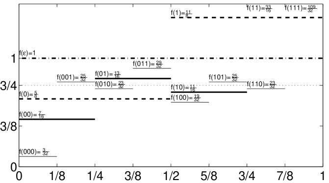
Figure 1: Construction of a martingale that with high probability converges to $\frac{3}{4}$ oscillating infinitely often.

It is obvious from the construction that $f(x_{1:t})$ is a martingale, it oscillates and converges to $\frac{3}{4}$ as $t\to\infty$ for all sequences $x_{<\infty}$ that always stay alive. The only thing we must show is that many sequences in fact stay alive.

Claim 20

We have $\lambda\big{(}\{x_{<\infty}:\ \exists t\;\mbox{ such that }\;x_{1:t}{\rm\ is\ dead}\}\big{)}\leq\frac{1}{4}$.

Proof. After the $n$th step, i.e. when $f$ has been defined for strings of length $n$, $f(x)$ assumes the value

$$a_{0}^{n}=\frac{3}{4}-2^{-n-2}$$

on a set of measure at most $\frac{1}{2}$. In the next step $n+1$, $f$ is defined to

$$a_{1}^{n}=\frac{3}{4}-2^{-n-1}\Big{(}1+\frac{1}{4}\Big{)}$$

on half of the extended strings. Generally, in the $k$th next step, $f$ is defined to

$$a_{k}^{n}=\frac{3}{4}-2^{-n+k-2}\Big{(}\sum_{j=0}^{k}2^{-2j}\Big{)}$$

on a $2^{-k}$ fraction of the extended strings.

The extended strings stay alive as long as $a_{k}^{n}\geq\frac{3}{8}+2^{-n-k-3}$ holds. Some elementary calculations show that this is equivalent to $k\leq n$. So precisely after $n+1$ additional steps, a fraction of $2^{-n-1}$ of the extended strings die.

We already noted that for $A_{n}=\{x:\ell(x)=n\wedge f(x)=a_{0}^{n}\}$, we have $\lambda(A_{n})\leq\frac{1}{2}$. Thus,

$$\lambda\big{(}\{x_{<\infty}:x_{1:n}\in A_{n}{\rm\ and\ }x_{1:2n+1}{\rm\ is\ dead}\}\big{)}\leq 2^{-n-2}.$$

Hence, one can conclude

$$\lambda\big{(}\{x_{<\infty}:\ \exists t\;\mbox{ such that }\;x_{1:t}{\rm\ is\ dead}\}\big{)}\leq\sum_{n=1}^{\infty}2^{-n-2}=\frac{1}{4},$$

which proves the claim. $\Box$

We now define the measure $\nu$ by

$$\nu(x)=f(x)\cdot\lambda(x)=f(x)\cdot 2^{-\ell(x)},$$

and set the weights to $w_{\lambda}=\frac{3}{7}$ and $w_{\nu}=\frac{4}{7}$. Then this provides an example where the maximizing element never stops oscillating with probability at least $\frac{3}{4}$.

Both examples point out different possible reasons for failure of stabilizing. Example 18 works since the measure $\mu$ and $\nu$ are asymptotically very similar and close to deterministic. In contrast, in Example 19 stabilizing fails because of lack of independence: The quantity $\nu(a|x)$ strongly depends on $x$. In particular, one can note that even Markovian dependence may spoil the stabilization, since $\nu(a|x)$ only depends on the last symbol of $x$.

7 Stabilization

In the light of the previous section, it is therefore natural to ask when the maximizing element stabilizes (almost surely). Barron [Bar85, BRY98] has shown that this happens if all distributions in $\mathcal{C}$ are asymptotically mutually singular. Under this condition, the true distribution is even eventually identified almost surely.

The condition of asymptotic mutual singularity holds in many important cases, e.g. if the distributions are i.i.d. However, one cannot always build on it. Therefore, in this section we give a different approach: In order to prevent stabilization, it is necessary that the ratio of two predictive distributions oscillates around the inverse ratio of the respective weights. Therefore, stabilization must occur almost surely if the ratio of two predictive distributions converges almost surely but is not concentrated in the limit. This is satisfied under appropriate conditions, as we will prove. We start with a general theorem which allows to conclude almost sure stabilization in a countable model class, if for any pair of models we have almost sure stabilization.

Theorem 21

Let $\mathcal{C}$ be a countable class of (semi)measures containing the true measure $\mu$. Assume that for each two $\nu_{1},\nu_{2}\in\mathcal{C}$ the maximizing element chosen from $\{\nu_{1},\nu_{2}\}$ eventually stabilizes almost surely. Then also the maximizing element chosen from all of $\mathcal{C}$ stabilizes almost surely.

Proof. It is immediate that the maximizing element chosen from any finite subset of $\mathcal{C}$ stabilizes almost surely. Now, for all $\nu\in\mathcal{C}$ and $c>0$, define the set $A_{c}^{\nu}$ by

$$A_{c}^{\nu}=\left\{x_{<\infty}:\exists\ t\geq 1\;\mbox{ such that }\;\frac{\nu(x_{1:t})}{\mu(x_{1:t})}\geq c\right\}.$$

Then we have

$$\mu(A_{c}^{\nu}) = \mu\left(\bigcup\Big{\{}\Gamma_{x}:\frac{\nu(x)}{\mu(x)}\geq c\wedge\frac{\nu(x_{1:s})}{\mu(x_{1:s})}<c\ \forall\ s<\ell(x)\Big{\}}\right)$$

$$= \sum\left\{\mu(x):\frac{\nu(x)}{\mu(x)}\geq c\wedge\frac{\nu(x_{1:s})}{\mu(x_{1:s})}<c\ \forall\ s<\ell(x)\right\}$$

$$\leq \sum\left\{\frac{\nu(x)}{c}:\frac{\nu(x)}{\mu(x)}\geq c\wedge\frac{\nu(x_{1:s})}{\mu(x_{1:s})}<c\ \forall\ s<\ell(x)\right\}$$

$$= \frac{1}{c}\sum\big{\{}\nu(x):\ldots\big{\}}\ \leq\ \frac{1}{c},$$

since $\nu$ is a (semi)measure and the set $\left\{x\in\mathcal{X}^{*}:\frac{\nu(x)}{\mu(x)}\geq c\wedge\frac{\nu(x_{1:s})}{\mu(x_{1:s})}<c\ \forall\ s<\ell(x)\right\}$ is prefix-free. Let

$$B^{\nu}=\left\{x_{<\infty}:\exists\ t\geq 1\;\mbox{ such that }\;\frac{w_{\nu}\nu(x_{1:t})}{w_{\mu}\mu(x_{1:t})}\geq 1\right\}=A_{(w_{\mu}/w_{\nu})}^{\nu},$$

then $\mu(B^{\nu})\leq\frac{w_{\nu}}{w_{\mu}}$ holds. We arrange the (semi)measures $\nu\in\mathcal{C}$ in an order $\nu_{1},\nu_{2},\ldots$ such that the weights $w_{\nu_{1}},w_{\nu_{2}},\ldots$ are descending. For each $c\geq 1$, we can now find an index $k$ and a set

$$\mathcal{N}_{c}=\{\nu_{i}:i\geq k\}\;\mbox{ such that }\;\sum_{\nu\in\mathcal{N}_{c}}w_{\nu}\leq\frac{w_{\mu}}{c}.$$

Defining $B_{c}=\bigcup_{\nu\in\mathcal{N}^{c}}B^{\nu}$, we get

$$\mu(B_{c})\leq\sum_{\nu\in\mathcal{N}^{c}}\frac{w_{\nu}}{w_{\mu}}\leq\frac{1}{c}.$$

For all $x_{<\infty}\notin B^{\nu}$, $\nu$ can never be the maximizing element. Therefore, for all $x_{<\infty}\notin B_{c}$, there are only finitely many $\nu\notin\mathcal{N}_{c}$ having the chance of becoming the maximizing element at any time. By assumption, the maximizing element chosen from the finite set $\mathcal{C}\setminus\mathcal{N}_{c}$ stabilizes a.s. Thus, we conclude almost sure stabilization on the sequences in $\mathcal{X}^{\infty}\setminus B_{c}$. Since this holds for all $B_{c}$ and $\mu(\mathcal{X}^{\infty}\setminus B_{c})\to 1$ as $c\to\infty$, the maximizing element stabilizes with $\mu$-probability one. $\Box$

For the rest of this section, we assume that the model class $\mathcal{C}$ contains only proper measures. A measure $\mu$ is called factorizable if there are measures $\mu_{i}$ on $\mathcal{X}$ such that

$$\mu(x)=\prod_{i=1}^{\ell(x)}\mu_{i}(x_{i})$$

for all $x\in\mathcal{X}^{*}$. That is, the symbols of sequences $x_{<\infty}$ generated by $\mu$ are independent. A factorizable measure $\mu=\prod\mu_{i}$ is called uniformly stochastic, if there is some $\delta>0$ such that at each time $i$ the probability of all symbols $a\in\mathcal{X}$ is either 0 or at least $\delta$. That is

$$\mu_{i}(a)>0\Rightarrow\mu_{i}(a)\geq\delta\;\mbox{ for all }\;a\in\mathcal{X}\;\mbox{ and }\;i\geq 1.$$ (27)

In particular, all deterministic measures and all i.i.d. distributions are uniformly stochastic. Another simple example of a uniformly stochastic measure is a probability distribution which generates alternately random bits by fair coin flips and the digits of the binary representation of $\pi=3.1415\ldots$

Lemma 22

Let $\mu$, $\nu$, and $\tilde{\nu}$ be factorizable and uniformly stochastic measures, where $\mu$ is the true distribution.
$(i)$ The maximizing element chosen from $\mu$ and $\nu$ stabilizes almost surely.
$(ii)$ If $\mu$ is not eventually always preferred over $\nu$ or $\tilde{\nu}$ (in which case we the maximizing element stabilizes a.s. by $(i)$), then the maximizing element chosen from $\nu$ and $\tilde{\nu}$ stabilizes almost surely.

Proof. We will show only $(ii)$, as the proof of $(i)$ is similar but simpler. So we assume that both $\nu$ and $\tilde{\nu}$ remain competitive in the process of choosing the maximizing element, and show that then maximizing element chosen from $\nu$ and $\tilde{\nu}$ stabilizes almost surely.

Let $\nu=\prod_{i}\nu_{i}$, $\tilde{\nu}=\prod_{i}\tilde{\nu}_{i}$, and $X_{i}=\frac{\tilde{\nu}_{i}(x_{i})}{\nu_{i}(x_{i})}$. The $X_{i}$ are independent random variables depending on the event $x_{<\infty}$. Moreover, both fractions $\frac{\nu(x_{1:t})}{\mu(x_{1:t})}$ and $\frac{\tilde{\nu}(x_{1:t})}{\mu(x_{1:t})}$ are martingales (with respect to $\mu$) and thus converge almost surely for $t\to\infty$. We are interested only in the events in

$$A_{\nu}=\left\{x_{<\infty}\in\mathcal{X}^{\infty}:{\textstyle\frac{\nu(x_{1:t})}{\mu(x_{1:t})}}{\rm\ converges\ to\ a\ value\ }>0\right\},$$

since otherwise $\nu$ eventually is no longer competitive. So we assume that $\mu(A_{\nu})>0$, which implies $\mu(A_{\nu})=1$ by the Kolmogorov zero-one-law (see e.g. [CT88]). Similarly, $\mu(A_{\tilde{\nu}})=1$ for the analogously defined set $A_{\tilde{\nu}}$. That is,

$$\prod_{i=1}^{t}X_{i}=\frac{\tilde{\nu}(x_{1:t})}{\nu(x_{1:t})}={\textstyle\frac{\tilde{\nu}(x_{1:t})}{\mu(x_{1:t})}}\Big{/}{\textstyle\frac{\nu(x_{1:t})}{\mu(x_{1:t})}}$$

converges to a value $>0$ almost surely, and in particular $0<X_{i}<\infty$ a.s.

Now we will use the concentration function of a real valued random variable $U$,

$$Q(U,\eta)=\sup_{u\in\mathbb{R}}\mu(u\leq U\leq u+\eta),\ \eta\geq 0.$$ (28)

This quantity was introduced by Lèvy, see e.g. [Pet95]. The concentration function is non-decreasing in $\eta$. Moreover, when two independent random variables $U$ and $V$ are added, we have [Pet95, Lemma 1.11]

$$Q(U+V,\eta)\leq\min\big{\{}Q(U,\eta),Q(V,\eta)\big{\}}\ \forall\ \eta\geq 0.$$ (29)

We first assume that the following set is unbounded:

$$B=\left\{\sum_{i=1}^{n}\Big{(}1-Q(X_{i},\eta)\Big{)}:n\in\mathbb{N},\eta>0\right\}\subset\mathbb{R}^{+},$$ that is (30)

$$\sup(B)=+\infty,$$ (31)

We show that then $\frac{\tilde{\nu}(x_{1:t})}{\nu(x_{1:t})}$ (which converges a.s.) is not concentrated in the limit. That is, it converges to some given $c>0$, in particular to $c=\frac{w_{\nu}}{w_{\tilde{\nu}}}$, with $\mu$-probability zero. This shows that almost surely it does not oscillate around $\frac{w_{\nu}}{w_{\tilde{\nu}}}$.

Define independent random variables $Y_{i}=\ln(X_{i})$. Let $S_{n}:=\sum_{1}^{n}Y_{i}$ and denote its almost everywhere existing limit by $S=\sum_{1}^{\infty}Y_{i}$. The assertion is verified under condition (31), if we can show that the distribution of $S$ is not concentrated to any point since then also $\prod_{1}^{\infty}X_{i}=\exp(S)$ is not concentrated to any point. In terms of the concentration function defined in (28), this reads $Q(S,0)=0$. According to (31), for each $R>0$, we find $\eta>0$ and $n\in\mathbb{N}$ such that $\sum_{i=1}^{n}\big{(}1-Q(X_{n},\eta)\big{)}>R$. Then, because of $X_{i}<\infty$ (ignoring the measure-zero set where this may fail),

$$W=\max_{1\leq i\leq n}X_{i}=\max\left\{{\textstyle\frac{\tilde{\nu}_{i}(x_{i})}{\nu_{i}(x_{i})}}:1\leq i\leq n{\rm\ and\ }\mu(x_{i})>0\right\}$$

is finite. The mapping

$$\big{(}0,W\big{]}\ni w\ \mapsto\ \ln(w)\in(-\infty,\ \ln W]$$

is bijective and has derivative at least $W^{-1}$. Let $\tilde{\eta}=\frac{\eta}{W}$. Then by definition of $Y_{i}$, we have $Q(Y_{i},\tilde{\eta})\leq Q(X_{i},\eta)$ for $1\leq i\leq n$ and consequently

$$\sum_{i=1}^{n}\Big{(}1-Q(Y_{i},\tilde{\eta})\Big{)}>R.$$

By the Kolmogorov-Rogozin inequality (see [Pet95, Theorem 2.15]), there is a constant $C$ such that

$$Q(S_{n},\tilde{\eta})\leq C\left(\sum_{i=1}^{n}\Big{(}1-Q(Y_{i},\tilde{\eta})\Big{)}\right)^{-\frac{1}{2}}.$$

Thus, for each $\varepsilon>0$, we can choose $R$ sufficiently large to guarantee $C\cdot R^{-\frac{1}{2}}<\varepsilon$. Then $Q(S_{n},\tilde{\eta})<\varepsilon$ for $n$ and $\tilde{\eta}$ as before. By (29) we conclude

$$Q(S,\tilde{\eta})=Q\left(S_{n}+\Big{(}\sum_{i=n+1}^{\infty}Y_{i}\Big{)},\tilde{\eta}\right)\leq Q(S_{n},\tilde{\eta})<\varepsilon$$

and consequently $Q(S,0)=0$ since $Q$ is non-decreasing. This proves the assertion under assumption (31).

Now assume that $B$ is bounded, i.e. (31) does not hold. Then there is $R>0$ such that $\sum_{1}^{n}\big{(}1-Q(X_{i},\eta)\big{)}\leq R$ for all $\eta>0$ and $n\in\mathbb{N}$. Since the distribution of $X_{i}$ is a finite convex combination of point measures, for each $i$ there is an $\eta>0$ such that $Q(X_{i},\eta)=Q(X_{i},0)$ and thus $\sum_{i=1}^{n}\big{(}1-Q(X_{i},0)\big{)}\leq R$ for all $n\in\mathbb{N}$. Therefore, also $\sum_{1}^{\infty}\big{(}1-Q(X_{i},0)\big{)}\leq R$ holds. Since $\tilde{\nu}_{i}(x_{i})=c_{i}\nu_{i}(x_{i})$ is equivalent to $X_{i}=c_{i}$, this implies that there are constants $c_{i}\geq 0$ such that

$$\sum_{i=1}^{\infty}\mu_{i}\big{\{}a:\tilde{\nu}_{i}(a)\neq c_{i}\nu_{i}(a)\big{\}}\leq R.$$ (32)

Next we argue that if $c_{i}\neq 1$ for infinitely many $i$, then either $\nu$ or $\tilde{\nu}$ is eventually not competitive. To verify this claim, let $N_{i}=\big{\{}a:\tilde{\nu}_{i}(a)\neq c_{i}\nu_{i}(a)\big{\}}$ and $M_{i}=\mathcal{X}\setminus N_{i}$ and observe that $\mu_{i}(N_{i})<\delta$ holds for sufficiently large $i$, since the sum (32) is bounded. On the other hand $\mu$ is uniformly stochastic, so there are no events of probability $\mu_{i}(a)\in(0,\delta)$, hence $\mu_{i}(N_{i})=0$ and $\mu_{i}(M_{i})=1$ for sufficiently large $i$. Now for these $i$, $c_{i}>1$ together with $\nu_{i}(M_{i})=1$ implies the contradiction $\tilde{\nu}_{i}(M_{i})=c_{i}>1$. So $c_{i}>1$ necessarily requires $\nu_{i}(M_{i})<1$, hence $\nu_{i}(M_{i})\leq 1-\delta$, since $\nu$ is uniformly stochastic. If this happens infinitely often, then $\nu$ is eventually not competitive. A symmetric argument with $\tilde{\nu}$ holds for $c_{i}<1$.

The last paragraph shows that, if both $\nu$ and $\tilde{\nu}$ stay competitive, eventually $\tilde{\nu}_{i}=\nu_{i}$ holds a.s. In this case, $\frac{\tilde{\nu}(x_{1:t})}{\nu(x_{1:t})}$ is eventually constant, which completes the proof. $\Box$

Corollary 23

Let $\mathcal{C}$ be a countable class of factorizable and uniformly stochastic measures, then the maximizing element stabilizes almost surely.

Proof. This follows from Theorem 21 and Lemma 22. $\Box$

Lemma 22 and Corollary 23 are certainly not the only or the strongest assertions obtainable for stabilization. They rather give a flavor how a proof can look like, even if the distributions are not asymptotically mutually singular. On the other hand, the given result is optimal at least in some sense, as shown by the previous Examples 18 and 19. In the former example, $\mu$ is not uniformly stochastic but both $\mu$ and $\nu$ are factorizable, while in the latter one, $\mu$ is uniformly stochastic but $\nu$ is not factorizable.

The proof of Lemma 22 crucially relies on the independence assumption, which is necessary in order to use the Kolmogorov-Rogozin inequality. It is possible to relax this and require independent sampling only “every so often”. It is however not clear how to remove this condition completely.

8 Applications

In the following, we present some applications of the theory developed so far. We begin by stating general loss bounds. After that, three very general applications are discussed.

8.1 Loss bounds

So far we have only considered special loss functions, like the square loss, the Hellinger loss, or the relative entropy. We now show how these results, in particular the bounds for the Hellinger loss, imply regret bounds for arbitrary loss functions. (As we will see, square distance is not sufficient.) This parallels the bounds in [Hut03a, Hut03b]. The proofs are simplified, in particular Lemma 24 facilitates the analysis considerably. The reader should compare the results to the bounds for “prediction with expert advice”, e.g. [CB97, HP05].

In order to keep things simple, we restrict to binary alphabet $\mathcal{X}=\{0,1\}$ in this section. Our results extend to general alphabet by the techniques used in [Hut03a]. Consider a binary predictor having access to a belief probability $\varphi$ depending on the current history, e.g. $\varphi(x_{t}=1|x_{<t})=\frac{1}{3}$. Which actual prediction should he output, 0 or 1? We can answer this question if we know the loss function, according to which losses are assigned to the (wrong) predictions. Consider for example the 0/1 loss (also known as classification error loss), i.e. a wrong prediction gives loss of 1 and a right prediction gives no loss. Then we should predict 1 if our belief is $\varphi>\frac{1}{2}$. This may be different under other loss functions. In general, we should predict in a Bayes optimal way: We should output the symbol with the least expected loss,

$$x^{\varphi}:=\mathop{\arg\min}_{\tilde{x}\in\{0,1\}}\{(1-\varphi)\ell(0,\tilde{x})+\varphi\ell(1,\tilde{x})\},$$

where $\ell(x,\tilde{x})$ is the loss incurred by prediction $\tilde{x}$ if the true symbol is $x$. In the following, we will restrict to bounded loss functions $\ell(x,\tilde{x})\in[0,1]$. Breaking ties in the above expression in an arbitrary deterministic way, the resulting prediction is deterministic for given $\varphi$ and loss function $\ell$. If $\mu$ is the true distribution as usual, then let $l^{\varphi}_{t}:=\sum_{a}\mu(a|x_{<t})\ell(a,x_{t}^{\varphi})$ be the $\mu$-expected loss of the $\varphi$-predictor. Then, by

$$L^{\varphi}_{1:n}={\mathbf{E}}[l_{1}^{\varphi}+...+l_{n}^{\varphi}]=\sum_{t=1}^{n}\mu(x_{<t})l_{t}^{\varphi}(x_{<t})$$

we denote the cumulative $\mu$-expected loss of the $\varphi$-predictor. With $\varphi$ being the variants of the MDL predictor, we will bound the quantity $\Delta_{1:n}=L^{\varphi}_{1:n}-L^{\mu}_{1:n}$, i.e. the cumulative regret, by an expression depending on $L^{\mu}_{1:n}$ and $w_{\mu}^{-1}$.

We admit arbitrary non-stationary loss functions $\ell_{x_{<t}}$ which may depend on the history. Our analysis considers the worst possible choice of loss functions and consists of three steps. First the cumulative regret bound is reduced to an instantaneous regret bound (Lemma 24). Then the instantaneous bound is reduced to a bound in terms of special functions of $\mu$ and $\varphi$ (Lemma 25). Finally, the bound for the special functions is given (Lemma 26).

Lemma 24

Assume that some $\varphi$-predictor satisfies the instantaneous regret bound $\delta_{t}=l_{t}^{\varphi}-l_{t}^{\mu}\leq 2h_{t}+2\sqrt{2h_{t}l_{t}^{\mu}}$, where $h_{t}=h_{t}(\mu,\varphi)$ is the Hellinger distance of the instantaneous predictive probabilities (23). Then the cumulative $\varphi$-regret is bounded in the same way:

$$\Delta_{1:n}=L^{\varphi}_{1:n}-L^{\mu}_{1:n}\leq 2H_{1:n}(\mu,\varphi)+2\sqrt{2H_{1:n}(\mu,\varphi)L^{\mu}_{1:n}}.$$

This and the following lemma hold with arbitrary constants, the choices $2$ and $2\sqrt{2}$ are the smallest ones for which Lemma 26 is true. Note that if the Hellinger distance is replaced by the relative entropy, then $2\sqrt{2}$ may be replaced by $2$. Thus, normalized dynamic MDL and Bayes mixture admit smaller bounds, compare [Hut03a]. However, this is not true for the other MDL variants, as we have no relative entropy bound there.

Proof. The key property is the super-additivity of the bound. A function $f:[0,\infty)^{2}\to[0,\infty)$ is said to be super-additive if

$$f(x_{1}+x_{2},y_{1}+y_{2})\geq f(x_{1},y_{1})+f(x_{2},y_{2}).$$

The function $(H,L)\mapsto\sqrt{HL}$ satisfies this condition. We now use an inductive argument. Assume $\Delta^{0}_{2:n}\leq 2H^{0}_{2:n}+2\sqrt{2H^{0}_{2:n}L^{\mu,0}_{2:n}}$, where the summation starts at $t=2$ and the superscript $0$ indicates that the first symbol of the sequence was $0$. Let the same hold for the first symbol $1$. Writing $\mu_{1}=\mu(1|\epsilon)$ and using $\delta_{1}\leq 2h_{1}+2\sqrt{2h_{1}l^{\mu}_{1}}$, we obtain

$$\Delta_{1:n}=\delta_{1}+(1-\mu_{1})\Delta^{0}_{2:n}+\mu_{1}\Delta^{1}_{2:n}$$

$$\leq 2\left[h_{1}+\sqrt{2h_{1}\ell_{1}}+(1-\mu_{1})\Big{(}H^{0}_{2:n}+\sqrt{2H^{0}_{2:n}L^{\mu,0}_{2:n}}\big{)}+\mu_{1}\Big{(}H^{1}_{2:n}+\sqrt{2H^{1}_{2:n}L^{\mu,1}_{2:n}}\Big{)}\right]$$

$$\leq 2\left[H_{1:n}+\sqrt{2h_{1}\ell_{1}}+\sqrt{2\Big{(}(1-\mu_{1})H^{0}_{2:n}+\mu_{1}H^{1}_{2:n}\Big{)}\Big{(}(1-\mu_{1})L^{\mu,0}_{2:n}+\mu_{1}L^{\mu,1}_{2:n}\Big{)}}\right]$$

$$\leq 2H_{1:n}+2\sqrt{2H_{1:n}L^{\mu}_{1:n}}.$$

Here, the first inequality is the induction hypothesis together with the instantaneous bound, the second bound is Cauchy-Schwarz’s inequality, and the last estimate is the super-additivity. $\Box$

Lemma 25

Assume that some $\varphi$-predictor satisfies $\tilde{\delta}\leq 2h+2\sqrt{2h\tilde{\ell}}$ for all $\mu,\varphi\in[0,1]$, with the Hellinger distance $h=h(\mu,\varphi)$ and the special functions $\tilde{\delta}(\mu,\varphi)$ and $\tilde{\ell}(\mu,\varphi)$ defined in the following way, where we slightly abuse notation and abbreviate $\mu=\mu(1|\ldots)$ and $\varphi=\varphi(1|\ldots)$:

$$\tilde{\delta}=\frac{|\varphi-\mu|}{\max\{\varphi,1-\varphi\}}\quad\;\mbox{ and }\;\quad\tilde{\ell}=\left\{\begin{array}[]{l @{\quad\mbox{if}\ } l}\mu&\mu\leq\varphi\leq\frac{1}{2},\\ \mu(1-\varphi)/\varphi&\mu\leq\varphi\wedge\frac{1}{2}\leq\varphi,\\ 1-\mu&\frac{1}{2}\leq\varphi\leq\mu,\\ (1-\mu)\varphi/(1-\varphi)&\varphi\leq\mu\wedge\varphi\leq\frac{1}{2}.\end{array}\right.$$

Then for arbitrary bounded loss function $\ell:\{0,1\}^{2}\to[0,1]$, we have

$$\delta\leq 2h+2\sqrt{2hl^{\mu}}.$$ (33)

Proof. First we show that we may assume $\ell(0,0)=\ell(1,1)=0$, i.e. we do not incur loss for correct predictions. To this end, consider the modified loss function $\ell^{\prime}(x,\tilde{x})=\ell(x,\tilde{x})-\ell(x,x)$ and assume w.l.o.g $\ell^{\prime}(x,\tilde{x})\in[0,1]$. Then it is not hard to see that the regrets under the original and the modified loss functions coincide, while the expected loss of the $\mu$-predictor clearly decreases with the modified loss function. Thus, (33) holds for $\ell$ if it holds for $\ell^{\prime}$. Hence we may assume $\ell(0,0)=\ell(1,1)=0$. For each possible outcome $x\in\{0,1\}$, we abbreviate $\ell^{x}=\ell(x,1-x)$.

Now assume w.l.o.g. $\mu\leq\varphi$. In order to show the assertion, we need to consider the cases in the definition of $\tilde{\ell}$ separately. We show this only for the first case, i.e. $\mu\leq\varphi\leq\frac{1}{2}$. Then $l^{\mu}=\mu\ell^{1}$, $l^{\varphi}=(1-\mu)\ell^{0}$. We assume that the $\mu$-predictor outputs 0 and the $\varphi$-predictor 1, otherwise they give the same prediction and the $\varphi$-predictor has no regret at all. This condition is equivalent to $\ell^{0}=\ell^{1}\frac{u}{1-u}$ for some $u\in[\mu,\varphi]$. We consider the worst case by maximizing $l^{\varphi}$, i.e. choosing $u$ as large as possible. For this $u=\varphi$, we obtain $\ell^{0}=\ell^{1}\frac{\varphi}{1-\varphi}$ and

$$\delta=\ell^{1}[{\textstyle\frac{(1-\mu)\varphi}{1-\varphi}}-\mu]=\ell^{1}\tilde{\delta}\leq\ell^{1}[2h+2\sqrt{2h\tilde{\ell}}]\leq 2h+2\sqrt{2h\ell^{1}\tilde{\ell}}\leq 2h+2\sqrt{2hl^{\mu}},$$

showing (33) provided that $\mu\leq\varphi\leq\frac{1}{2}$. The other cases are shown similarly. $\Box$

Lemma 26

The bound $\tilde{\delta}\leq 2h+2\sqrt{2h\tilde{\ell}}$ holds for all $\mu,\varphi\in[0,1]$, with the functions $\tilde{\delta},\tilde{\ell}:[0,1]^{1}\to[0,1]$ as defined in Lemma 25.

The technical and not very interesting proof of this lemma is omitted. The careful reader may check the assertion numerically or graphically, as it is just the boundedness of some function on the unit square. We remark that the bound does not hold if the Hellinger distance is replaced by the quadratic distance, not even with larger constants.

Theorem 27

For arbitrary non-stationary loss function which is bounded in $[0,1]$ and known to the MDL predictors, their respective losses are bounded by

$$L^{\varrho_{\mathrm{norm}}}_{1:n},L^{\varrho}_{1:n},L^{\varrho^{\mathrm{static}}}_{1:n},L^{\varrho^{\mathrm{static}}_{\mathrm{norm}}}_{1:n}\quad\leq\quad L^{\mu_{\mathrm{norm}}}_{1:n}+2\sqrt{2cL^{\mu_{\mathrm{norm}}}_{1:n}\cdot w_{\mu}^{-1}}+2cw_{\mu}^{-1},$$

where the constant $c=2,8,21,\mbox{ or }32$, according to which MDL predictor is used (compare Corollary 14).

Proof. This follows from the above three lemmas and from $H_{1:n}\leq c\!\cdot\!w_{\mu}^{-1}$ (Corollary 14). $\Box$

This shows in particular that, regardless of the loss function, the average expected per-round regret tends to zero. Again, the direct practical relevance of the bounds is limited because of the potentially huge $w_{\mu}^{-1}$.

8.2 Classification

Transferring our results to pattern classification is very easy. All we have to do is to add inputs to our models. That is, we consider an arbitrary input space $\mathcal{U}$ and (as before) a finite observation or output space $\mathcal{X}$. A model is now a measure

$$\nu(x|u)\in[0,1],\ x\in\mathcal{X},\ u\in\mathcal{U},\mbox{ where }\sum_{x\in\mathcal{X}}\nu(x|u)=1\;\mbox{ for all }\;u\in\mathcal{U}.$$

That is, we have a distribution which is conditionalized to the input. We restrict our discussion to measures, since there is no motivation to consider semimeasures for classification. The definition of a model does not include history dependence. There is no loss of generality: We may include the history in the arbitrary input space.

Transferring the proofs in the previous sections to the present setup is straightforward. We therefore obtain immediately the following corollaries.

Corollary 28

Let $\mathcal{C}$ be a countable set of classification models containing the true distribution $\mu$. Then for any sequence of inputs $u_{<\infty}\in\mathcal{U}$, we have

$$\begin{array}[]{l @{\quad} c @{\quad} l}\sum_{t}{\mathbf{E}}\sum_{a}\big{(}\mu(a|u_{t})-\varrho_{\mathrm{norm}}(a|u_{t},u_{<t},x_{<t})\big{)}^{2}&\leq&2w_{\mu}^{-1},\\[3.0pt] \sum_{t}{\mathbf{E}}\sum_{a}\big{(}\mu(a|u_{t})-\varrho(a|u_{t},u_{<t},x_{<t})\big{)}^{2}&\leq&8w_{\mu}^{-1},\\[3.0pt] \sum_{t}{\mathbf{E}}\sum_{a}\big{(}\mu(a|u_{t})-\varrho^{\mathrm{static}}(a|u_{t},u_{<t},x_{<t})\big{)}^{2}&\leq&21w_{\mu}^{-1}.\end{array}$$

(Note that although each single model formally does not depend on the history, the MDL estimators necessarily do.)

We need not consider the normalized static variant here, since all models are measures anyway. If there is a distribution over $\mathcal{U}$, the result therefore also holds in expectation over the inputs. An analogue of Corollary 23 is obtained as easily. If the inputs are i.i.d., which is usually assumed for classification, then the two conditions of factorizability and uniform stochasticity are trivially satisfied. Therefore, the true distribution $\mu$ is eventually discovered by MDL almost surely. Note that in this case, the distributions are also asymptotically mutually singular, so that the assertion also follows from Barron’s [Bar85] earlier result.

Note that again, the assumption $\mu\in\mathcal{C}$ is essential. In practical applications, if this is not clear, it may be therefore favorable to choose a different method having guarantees without this condition, compare [GL04].

8.3 Regression

We may also apply our results in the regression setup, that is for predicting continuous densities. Our use of the term regression is a bit non-standard here, since it normally refers to just estimating the mean of some prediction, where the distribution is often assumed to be Gaussian. Again the assumption $\mu\in\mathcal{C}$ is essential, so that in practice some other method not relying on it might be preferred.

Continuous densities cause some additional difficulties. The observation space is now $\mathbb{R}$. This implies in particular that, like for the loss bounds, the square distance is no longer appropriate for our purpose (note that our use of the squared error is completely different from the standard use in regression). So we will use the Hellinger distance instead, defined similarly to (23) by

$$h(f,\tilde{f})=\int\Big{(}\sqrt{f(x)}-\sqrt{\tilde{f}(x)}\Big{)}^{2}dx\mbox{\quad for integrable }f,\tilde{f}:\mathbb{R}\to[0,\infty).$$ (34)

Accordingly, $H_{1:n}(\mu,\varphi)=\sum_{t}{\mathbf{E}}h\big{(}\mu(\cdot|u_{t}),\varphi(\cdot|u_{t},u_{<t},x_{<t})\big{)}$ is the cumulative Hellinger distance of two predictive distributions $\mu$ and $\varphi$. Similarly as in (25) and (26), the Hellinger distance is bounded by the (continuous) relative entropy and absolute distance. This shows in particular that the integral (34) exists.

We now consider a countable class $\mathcal{C}$ of models that are functions $\nu$ from $\mathcal{U}$ to uniformly bounded probability densities on $\mathcal{X}=\mathbb{R}$. That is, there is some $C>0$ such that

$$0\leq\nu_{i}(x|u)\leq C\;\mbox{ and }\;\int_{-\infty}^{\infty}\nu_{i}(x|u)dx=1\;\mbox{ for all }\;i\geq 1,\ u\in\mathcal{U},\;\mbox{ and }\;x\in\mathbb{R}.$$ (35)

for all $i\geq 1$, $u\in\mathcal{U}$, and $x\in\mathbb{R}$. The MDL estimator is then defined as the element which maximizes the density, $\nu^{*}=\arg\max_{\nu\in\mathcal{C}}\{w_{\nu}\nu(x_{1:n}|u_{1:n})\}$. The uniform boundedness condition asserts that the MDL estimator exists. It may be relaxed, provided that the MDL estimator remains well-defined, such as for a family of Gaussian densities which tend to the point measure.

With these definitions, the proofs of the theorems for static and dynamic MDL can be adapted. Since the triangle inequality holds for the Hellinger distance $\sqrt{H^{2}}$, we obtain the following.

Corollary 29

Let $\mathcal{C}$ be a countable model class according to (35), containing the true distribution $\mu$. Then for any sequence of inputs $u_{<\infty}\in\mathcal{U}$, we have $H_{1:n}(\mu,\varrho_{\mathrm{norm}})\leq 2w_{\mu}^{-1}$, $H_{1:n}(\mu,\varrho)\leq 8w_{\mu}^{-1}$, and $H_{1:n}(\mu,\varrho^{\mathrm{static}})\leq 21w_{\mu}^{-1}$.

We may apply this for example to model classes with Gaussian noise, concluding that the mean and the variances converge to the true values, see [PH05] for an example. It is not immediately clear how to obtain an analogue of Corollary 23 for continuous densities.

8.4 Universal Induction

Since the assertions on static and dynamic MDL have been proven generally for semimeasures, we may apply them to the universal setup. Here $\mathcal{C}=\mathcal{M}$ is the countable set of all lower semicomputable (= enumerable) semimeasures on $\mathcal{X}^{*}$. So $\mathcal{M}$ contains stochastic models in general, and in particular all models for computable deterministic sequences. There is a one-to-one correspondence of $\mathcal{M}$ to the class of all programs on some fixed universal monotone Turing machine $U$, see e.g. [LV97]. We will assume programs to be binary, in contrast to outputs, which are strings $x\in\mathcal{X}^{*}$. This relation defines in particular the complexities and weights of each $\nu$ by

$$K\!w(\nu)=\mbox{length of the program for $\nu$ on $U$},\;\mbox{ and }\;w_{\nu}=2^{K\!w(\nu)}.$$ (36)

We call these weights the canonical weights. They satisfy $w_{\nu}>0$ for all $\nu$ and $\sum_{\nu}w_{\nu}\leq 1$.

An enumerable semimeasure which dominates all other enumerable semimeasures is called universal. The Bayes mixture $\xi$ defined in (2) has this property. One can show that $\xi$ is equal within a multiplicative constant to Solomonoff’s prior [Sol64, Eq. (7)], which is the a priori probability that (some extension of) a string $x$ is generated provided that the input of $U$ consists of fair coin flips. That is

$$\xi(x)\quad\stackrel{{\scriptstyle\times}}{{=}}\quad M(x)\quad=\quad\sum_{\hbox to0.0pt{$\scriptstyle p\ minimal:\ U(p)=x*$\hss}}2^{-\ell(p)}\;\mbox{ for all }\;x\in\mathcal{X}^{*}.$$

Here, we use the notations

$$f\stackrel{{\scriptstyle+}}{{\leq}}g:\Leftrightarrow f\leq g+O(1), f\stackrel{{\scriptstyle+}}{{=}}g:\Leftrightarrow f\stackrel{{\scriptstyle+}}{{\leq}}g\wedge g\stackrel{{\scriptstyle+}}{{\leq}}f,$$

$$f\stackrel{{\scriptstyle\times}}{{\leq}}g:\Leftrightarrow f\leq g\cdot O(1), f\stackrel{{\scriptstyle\times}}{{=}}g:\Leftrightarrow f\stackrel{{\scriptstyle\times}}{{\leq}}g\wedge g\stackrel{{\scriptstyle\times}}{{\leq}}f.$$

The MDL definitions in Section 3 directly transfer to this setup. All bounds on the cumulative square loss (subsumed in Corollary 14) therefore apply to $\varrho=\varrho_{[\mathcal{M}]}$. The necessary assumption now reads that $\mu$ must be a recursive (= computable) measure. Also, Theorem 1 implies Solomonoff’s important universal induction theorem.

In addition to $\mathcal{M}$, we also consider the set of all recursive measures $\tilde{\mathcal{M}}$ together with the same canonical weights (36). We define $\tilde{\xi}=\xi_{[\tilde{\mathcal{M}}]}$ and $\tilde{\varrho}=\varrho_{[\tilde{\mathcal{M}}]}$. Then $\tilde{\varrho}(x)\leq\tilde{\xi}(x)\leq\xi(x)$ and $\varrho(x)\leq\xi(x)$ for all $x\in\mathcal{X}^{*}$ is immediate. It is straightforward that $\xi(x)\stackrel{{\scriptstyle\times}}{{\leq}}\varrho(x)$ since $\xi\in\mathcal{M}$. Moreover, for any string $x\in\mathcal{X}^{*}$, define the monotone complexity $K\!m(x)=\min\{\ell(p):U(p)=x*\}$ as the length of the shortest program such that $U$’s output starts with $x$. The following assertion holds.

Proposition 30

We have $K\!\tilde{\varrho}\stackrel{{\scriptstyle+}}{{\geq}}K\!m$.

Proof. We must show that given a string $x\in\mathcal{X}^{*}$ and a recursive measure $\nu$ (which in particular may be the MDL descriptor $\nu^{*}(x)$) it is possible to specify a program $p$ of length at most $K\!w(\nu)+K\!\nu(x)+c$ that outputs a string starting with $x$, where constant $c$ is independent of $x$ and $\nu$.

Consider all strings $y_{i}\in\mathcal{X}^{n}$ ($1\leq i\leq|\mathcal{X}|^{n}$) of length $n=\ell(x)$ arranged in lexicographical order. Each $y_{i}$ has measure $P_{i}=\mu(y_{i})$. Let $S_{i}$ be the cumulated measures: $S_{0}=0$ and $S_{i}=\sum_{k=1}^{i}P_{k}$. Let $j$ be the index of $x$, i.e. $x=y_{j}$. Then, the interval $[S_{j-1},S_{j})\subset[0,1)$ has measure $P_{j}$ and therefore contains exactly one $\lceil-{\log_{2}}P_{j}\rceil$-bit number $z\in[S_{j-1},S_{j})$. We describe $x$ with the number $z$, this is known as arithmetic encoding (see e.g. [CT91]). The coding is injective since $[S_{i-1},S_{i})$ and $[S_{k-1},S_{k})$ are disjoint for $i\neq k$.

In order to decode $z$, we may descend the $|\mathcal{X}|$-ary tree of all possible strings $y$, first considering strings of length one, then of length two, etc. For each possible string $y$, we can determine its binary code by approximating $\nu(x)$ sufficiently accurately. Eventually we will find $z$, then we print the current $y$. At this stage, $y$ might be only a prefix of $x$, since an extension of $y$ might have a measure very close to $y$ and thus map to the same code $z$. Therefore we continue the procedure until all codes starting with $z$ are proper extensions of $z$ (which may never be the case, then the algorithm runs forever). In each step, the appropriate additional symbol is written on the output tape. The resulting output will be $x$ or some extension of $x$.

This algorithm can be specified in a constant $c^{\prime}$ number of bits. The description of $\nu$ needs another $K\!w(\nu)$ bits. Finally, $z$ has length $\lceil-{\log_{2}}P_{j}\rceil\leq-{\log_{2}}\nu(x)+1$. Thus, the overall description has length $K\!w(\nu)+K\!\nu(x)+c$ as required. $\Box$

It is also possible to prove the proposition indirectly using [LV97, Thm.4.5.4]. This implies that $K\!m(x)\stackrel{{\scriptstyle+}}{{\leq}}K\!w(\nu)+K\!\nu(x)$ for all $x\in\mathcal{X}^{*}$ and all recursive measures $\nu\in\tilde{\mathcal{M}}$. Then, also $K\!m(x)\stackrel{{\scriptstyle+}}{{\leq}}\min\{K\!w(\nu)+K\!\nu(x)\}=K\!\tilde{\varrho}(x)$ holds.

So together with the above observations, we have

$$K\!m(x)\ \stackrel{{\scriptstyle+}}{{\leq}}\ K\!\tilde{\varrho}(x)\ \stackrel{{\scriptstyle+}}{{\geq}}\ K\!\tilde{\xi}(x)\ \stackrel{{\scriptstyle+}}{{\geq}}\ K\!\varrho(x)\ \stackrel{{\scriptstyle+}}{{=}}\ K\!M(x).$$ (37)

On the other hand, there is a deep result in Algorithmic information theory which states that an exact coding theorem does not hold on continuous sample space, $K\!m(x)\stackrel{{\scriptstyle+}}{{\gneq}}K\!M(x)$ [Gác83]. Therefore, at least one of the above $\stackrel{{\scriptstyle+}}{{\geq}}$ must be proper.

Problem 31

Which of the two inequalities $K\!\tilde{\varrho}(x)\stackrel{{\scriptstyle\times}}{{\geq}}K\!\tilde{\xi}(x)$ and $K\!\tilde{\xi}(x)\stackrel{{\scriptstyle\times}}{{\geq}}K\!\varrho(x)$ is proper (or are both)?

The proof in [Gác83] is very subtle, and the phenomenon is still not completely understood. There is some hope that by answering Problem 31, one arrives at a better understanding of the continuous coding theorem and even at a simpler proof for its failure.

9 Discussion

In this last section, we recapitulate the main achievements of this work and discuss their philosophical and practical consequences. In the first place, we have shown that if two-part MDL is used for predicting a stochastic sequence, then the predictive probabilities converge to the true ones in mean sum, provided that the distribution generating the sequence is contained in the model class. The two most important implications are almost sure convergence and loss bounds for arbitrary loss functions.

The guaranteed convergence is slow in general: All bounds depend linearly on $w_{\mu}^{-1}$, the inverse of the prior weight of the true distribution. For large model classes, this number must be regarded too huge to be relevant for practical applications. Examples show that this bound is sharp. This is in contrast to the exponentially smaller corresponding bound for the Bayes mixture. The latter predictor however is often computationally more expensive to approximate in practice. We believe that this principally indicates that with MDL, some care has to be taken when choosing the model class and the prior. Conditions which are sufficient for fast convergence have been given for instance in [Ris96, BRY98, PH04b]. It remains a major challenge to generalize these results in order to obtain fast convergence under assumptions that are as weak as possible. In particular for universal induction, this question is interesting and possibly difficult. Even when considering only computable Bernoulli distributions endowed with a universal prior, fast convergence possibly holds for many environments, but maybe not for all [PH04b]. We also need to distinguish how the large error cumulates. Either the instantaneous error remains significant for a long time, which is critical, or the instantaneous error drops just too slowly to be summable, e.g. as $O(\frac{1}{n})$, which is tolerable. We have seen instances for both cases; compare the discussion after Example 15. In this light, the cumulative error might not be the right quantity to assess convergence speed.

The main results have been shown under the only assumption that the data generating process is contained in the model class. This condition is essential in general, as [GL04] shows that in its absence MDL can fail dramatically. In the universal setup, the assumption merely requires that the data is generated in some (probabilistically) computable way. This is a very weak condition. Laplace, Zuse [Zus67] and successors argue that nature operates in a computable way, and consequently all thinkable data satisfies the assumption. On the other hand, predicting with a universal model is computationally very expensive. In particular it is provably infeasible if the thesis of computable nature holds. Despite these practical problems, the theory of universal prediction is valuable since it explores the limits of computational induction.

Acknowledgements. Thanks to Peter Grünwald and an anonymous reviewer for their very valuable comments and suggestions. This work was supported by SNF grant 2100-67712.02.

References

- [Bar85] A. R. Barron. Logically smooth density estimation. PhD thesis, Dept. of Electrical Engineering, Stanford University, 1985.
- [BC91] A. R. Barron and T. M. Cover. Minimum complexity density estimation. IEEE Trans. on Information Theory, 37(4):1034–1054, 1991.
- [BD62] D. Blackwell and L. Dubins. Merging of opinions with increasing information. Annals of Mathematical Statistics, 33:882–887, 1962.
- [BRY98] A. R. Barron, J. J. Rissanen, and B. Yu. The minimum description length principle in coding and modeling. IEEE Trans. on Information Theory, 44(6):2743–2760, 1998.
- [Cal02] C. S. Calude. Information and Randomness. Springer, Berlin, 2nd edition, 2002.
- [CB90] B. S. Clarke and A. R. Barron. Information-theoretic asymptotics of Bayes methods. IEEE Trans. on Information Theory, 36:453–471, 1990.
- [CB97] N. Cesa-Bianchi et al. How to use expert advice. Journal of the ACM, 44(3):427–485, 1997.
- [CT88] Y. S. Chow and H. Teicher. Probability Theory. Springer-Verlag, New York, 2nd edition, 1988.
- [CT91] T. M. Cover and J. A. Thomas. Elements of Information Theory. Wiley Series in Telecommunications. John Wiley & Sons, New York, NY, USA, 1991.
- [Doo53] J. L. Doob. Stochastic Processes. John Wiley & Sons, New York, 1953.
- [Gác83] P. Gács. On the relation between descriptional complexity and algorithmic probability. Theoretical Computer Science, 22:71–93, 1983.
- [GL04] P. Grünwald and J. Langford. Suboptimal behaviour of Bayes and MDL in classification under misspecification. In 17th Annual Conference on Learning Theory (COLT), pages 331–347, 2004.
- [Grü98] P. D. Grünwald. The Minimum Discription Length Principle and Reasoning under Uncertainty. PhD thesis, Universiteit van Amsterdam, 1998.
- [GV01] S. Ghosal and A. van der Vaart. Entropies and rates of convergence for Bayes and maximum likelihood estimation for mixture of normal densities. Ann. Statist., 29(5):1233–1263, 2001.
- [GV04] S. Ghosal and A. van der Vaart. Convergence rates of posterior distributions for noniid observations. preprint, 2004.
- [HP05] M. Hutter and J. Poland. Adaptive online prediction by following the perturbed leader. Journal of Machine Learning Research, 6:639–660, 2005.
- [Hut01] M. Hutter. New error bounds for Solomonoff prediction. Journal of Computer and System Sciences, 62(4):653–667, June 2001.
- [Hut03a] M. Hutter. Convergence and loss bounds for Bayesian sequence prediction. IEEE Trans. on Information Theory, 49(8):2061–2067, 2003.
- [Hut03b] M. Hutter. Optimality of universal Bayesian prediction for general loss and alphabet. Journal of Machine Learning Research, 4:971–1000, 2003.
- [Hut03c] M. Hutter. Sequence prediction based on monotone complexity. In Proc. 16th Annual Conference on Learning Theory (COLT-2003), Lecture Notes in Artificial Intelligence, pages 506–521, Berlin, 2003. Springer.
- [Hut04] M. Hutter. Universal Artificial Intelligence: Sequential Decisions based on Algorithmic Probability. Springer, Berlin, 2004. 300 pages, http://www.idsia.ch/marcus/ai/uaibook.htm.
- [LCL+03] M. Li, X. Chen, X. Li, B. Ma, and P. M. B. Vitányi. The similarity metric. In Proc. 14th ACM-SIAM Symposium on Discrete Algorithms (SODA), 2003.
- [Li99] J. Q. Li. Estimation of Mixture Models. PhD thesis, Dept. of Statistics. Yale University, 1999.
- [LV97] M. Li and P. M. B. Vitányi. An introduction to Kolmogorov complexity and its applications. Springer, 2nd edition, 1997.
- [Pet95] V. V. Petrov. Limit Theorems of Probability Theory. Clarandon Press, Oxford, 1995.
- [PH04a] J. Poland and M. Hutter. Convergence of discrete MDL for sequential prediction. In 17th Annual Conference on Learning Theory (COLT), pages 300–314, 2004.
- [PH04b] J. Poland and M. Hutter. On the convergence speed of MDL predictions for Bernoulli sequences. In International Conference on Algorithmic Learning Theory (ALT), pages 294–308, 2004.
- [PH05] J. Poland and M. Hutter. Strong asymptotic assertions for discrete MDL in regression and classification. In Benelearn 2005 (Ann. Machine Learning Conf. of Belgium and the Netherlands), 2005.
- [Ris78] J. J. Rissanen. Modeling by shortest data description. Automatica, 14:465–471, 1978.
- [Ris96] J. J. Rissanen. Fisher Information and Stochastic Complexity. IEEE Trans. on Information Theory, 42(1):40–47, January 1996.
- [Sol64] R. J. Solomonoff. A formal theory of inductive inference: Part 1 and 2. Inform. Control, 7:1–22, 224–254, 1964.
- [Sol78] R. J. Solomonoff. Complexity-based induction systems: comparisons and convergence theorems. IEEE Trans. Information Theory, IT-24:422–432, 1978.
- [VL00] P. M. Vitányi and M. Li. Minimum description length induction, Bayesianism, and Kolmogorov complexity. IEEE Trans. on Information Theory, 46(2):446–464, 2000.
- [WB68] C. S. Wallace and D. M. Boulton. An information measure for classification. Computer Jrnl., 11(2):185–194, August 1968.
- [Zha04] T. Zhang. On the convergence of MDL density estimation. In Proc. 17th Annual Conference on Learning Theory (COLT), pages 315–330, 2004.
- [ZL70] A. K. Zvonkin and L. A. Levin. The complexity of finite objects and the development of the concepts of information and randomness by means of the theory of algorithms. Russian Mathematical Surveys, 25(6):83–124, 1970.
- [Zus67] K. Zuse. Rechnender Raum. Elektronische Datenverarbeitung, 8:336–344, 1967. English translation: Calculating Space, MIT Technical Translation AZT-70-164-GEMIT, 1970.