HepToX: Heterogeneous Peer to Peer XML Databases 

Abstract

We study a collection of heterogeneous XML databases maintaining similar and related information, exchanging data via a peer to peer overlay network. In this setting, a mediated global schema is unrealistic. Yet, users/applications wish to query the databases via one peer using its schema. We have recently developed HepToX, a P2P Heterogeneous XML database system. A key idea is that whenever a peer enters the system, it establishes an acquaintance with a small number of peer databases, possibly with different schema. The peer administrator provides correspondences between the local schema and the acquaintance schema using an informal and intuitive notation of arrows and boxes. We develop a novel algorithm that infers a set of precise mapping rules between the schemas from these visual annotations. We pin down a semantics of query translation given such mapping rules, and present a novel query translation algorithm for a simple but expressive fragment of XQuery, that employs the mapping rules in either direction. We show the translation algorithm is correct. Finally, we demonstrate the utility and scalability of our ideas and algorithms with a detailed set of experiments on top of the Emulab, a large scale P2P network emulation testbed.

1 Introduction

Consider a large scale data sharing setting where several XML data sources in a similar domain (e.g., hospitals/medical centers) need to share (parts of) their data. The source schemas can be quite different. Figure 1 shows an example of two hospital DTDs expressed as graphs, adapted from [18]. (See [3, 17] for similar healthcare examples of P2P DBMS.) Ignore the cross arrows linking the DTDs for now. The first DTD shows how information is represented in the Montreal General Hospital database. Every patient is assigned a unique ID by the hospital and has a unique Medicare number (MedCr#). Note that symptoms of problems experienced by patients and the treatments they are administered are all grouped under patients. Data pertaining to patient admissions is maintained separately and is captured via the ID/IDREF link @PatRef$\,\rightarrow\,$@ID (shown as a solid grey arrow in Figure 1).

On the other hand, a patient who is moved from Montreal to Boston needs to establish early enough an acquaintance with the Mass General Hospital schema. Indeed, the patient database at the Mass General Hospital in Boston is organized quite differently. In this schema, at admission time patients are classified on the basis of their main complaint (pulmonary, coronary, or other illnesses not shown in the figure). Under this classification, the usual patient details such as name, hospital ID, insurance number, insurer, admission and discharge dates are stored. Progress of patients during their stay in the hospital is recorded: patients’ history of health problems as well as the treatments administered are tracked. All of this information is connected to the patients via the ID/IDREF link @PatRef$\,\rightarrow\,$@ID (solid grey arrow, Figure 1).

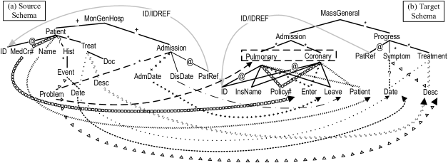
Figure 1: Mapping two Heterogeneous Peer DTDs. To minimize clutter, some arrows between corresponding tags have been omitted (e.g., @ID to @ID); every unlabeled edge is labeled ‘1’ by default.

Suppose we have several heterogeneous schemas, which describe the data of several health/medical data sources. A natural strategy for data exchange between the sources is to embed them in a loosely coupled environment. The loose coupling is crucial for allowing maximum flexibility, with no hard commitments to conform to any rigid requirements. Currently, there is significant interest in peer-to-peer (P2P) database systems [2, 3, 5, 14, 18, 20, 24]. A P2P database system is essentially a collection of autonomous database systems connected by a P2P network, with the flexibility that peers may enter or leave the network at will. In this paper, we assume that any peer at the time of entering the P2P network provides a mapping between its schema and a small number of the existing peer schemas. The peers chosen by the entering peer are called its acquaintances [2]. E.g., the Montreal General peer may provide “correspondences” between the concepts (elements and attributes) in its schema and those in the Mass General schema. The next question is who will provide this mapping and how. We could make use of (semi-)automatic schema mapping tools [9, 21, 13]. However, one might wish to customize or even override the associations produced by these tools. To allow for this, we consider a model where a peer database administrator supplies simple and intuitive correspondences between the peer schema and a small number of acquaintance schemas. The correspondences are specified in the form of arrows and boxes, illustrated in Figure 1, and will be explained in Section 2. We use the correspondences as a basis for automatically inferring a mapping expression, expressed in the form of Datalog-like rules. The peer DBA may (but doesn’t have to) examine the rules and make any necessary adjustments. In this way, joining a P2P DBMS is made a lightweight operation.

There may be considerable differences in the way the peers organize their data, including differences in data representations (e.g., stock names instead of ticker symbols, different units, etc.), as well as differences in underlying schemas (e.g., group treatments under the patients receiving them as opposed to maintaining separate lists of patients and treatments and linking them with ID/IDREF links). Differences in data representation were addressed by previous work [14] by introducing the so-called mapping tables. These are aimed at mapping value aliases in P2P networks, which are orthogonal to schema mappings. Differences in schemas have also been studied in Clio [20] and in Piazza [3, 4]. However, [20] focuses on deriving mappings across schemas and uses them to translate the data accordingly. Query translation across the inferred mappings is not considered. Furthermore, the kind of heterogeneity addressed in [20] is limited. Piazza [3, 4] addresses the schema mediation problem within a community of peers, where entering peers establish semantic mappings with existing peers, in an XQuery-like language. Our mappings are to be considered in a large P2P framework. For this reason, we do not expect a peer DBA/user to know the rule machinery at all, whereas it is reasonable to assume s/he can draw arrows and boxes. Piazza is again limited in the extent of schema heterogeneity it can handle. A detailed comparison with this and other related work appears in Section 6.

Our further goal is to permit users and applications of any peer database to access data items of interest by simply posing a query to their peer, regardless of the location of the data items or the schema under which they are organized. In other words, the existence of numerous peers and their schemas should all be transparent to the user/application posing the query. E.g., for answering the query “what are the treatments administered to patients admitted with a coronary illness?”, we want to manipulate data from all peers “visible” to the original peer, containing logically relevant information. Clearly, queries posed to a peer need to be translated appropriately so as to run on other peers.

The major challenges we address are the following: (1) How do we cope with the heterogeneity in the peer schemas in the context of P2P data sharing? (2) What is the exact semantics for the evaluation of peer queries, and how do we translate queries across peers, given the heterogeneity of their schemas? (3) How can we evaluate queries correctly and efficiently over the network?

Summarizing, we make the following contributions.

• We assume correspondences between a pair of peer DTDs are specified diagrammatically. We develop a novel algorithm for inferring mappings between the DTDs, couched in the form of Datalog-like rules and discuss the significance of the class of transformations captured by the rules (Section 3).

• We define the semantics of peer queries. We develop a novel query translation algorithm that handles a simple but significant fragment of XQuery and show that it is correct w.r.t. the above semantics. We illustrate our algorithm with examples (Section 4). Translation is non-trivial even for the XQuery fragment considered.

• We have developed HepToX, a HEterogeneous Peer TO peer Xml database system, incorporating the ideas developed in this paper. We describe our implementation of HepToX, including the strategies employed for efficient query evaluation. We ran an extensive set of experiments to measure the effectiveness of our query translation algorithm, as well as the scalability of our approach. We discuss the results and the lessons learned (Section 5).

Section 2 gives a motivating example. Related work is discussed in Section 6, while Section 7 summarizes the paper and discusses future research.

2 A Motivating Example

Revisit the example discussed in the introduction (Figure 1). The arrows provide informal correspondences between the two hospital DTDs, and are illustrated with different types of arrows, for clarity. Henceforth we refer to the Montreal General DTD as MonG and the Mass General DTD as MasG. The arrows capture simple 1-1 correspondences between terms such as “MedCr# in the first DTD to Policy# in the second” and “Name in the first to Patient in the second”. The correspondences can be naturally understood as propagating from the leaves up to the their parent/ancestor elements as in [9]. Arrows between leaf elements of tree DTDs have a straightforward meaning. Since our DTDs are DAGs, we use different arrow types for disambiguation. E.g., consider the correspondence between Desc in the two DTDs. Desc has a unique parent in first DTD while it has two parents in the second. For disambiguation, we use the same arrow type for the edges Treat/Desc in MonG, Treatment/Desc in MasG, and the arrow connecting them. Similarly, we use the same arrow type for the edges Event/Problem in MonG, Symptom/Desc in MasG, and the arrow connecting them. Other arrows can be understood similarly. E.g., Event/Date and Treat/Date are matched to their counterparts in the second DTD. Finally, consider the (thick dashed) box enclosing the Pulmonary and Coronary nodes. There is a thick dashed arrow matching Admission/Problem to this box. What it says is that ‘Pulmonary’ and ‘Coronary’ correspond to values of the element Admission/Problem in the first database. Again, recall there may be other illnesses (corresponding to values of Admission/Problem) not shown in the figure for brevity. In effect, illnesses which may be instances of Admission/Problem in the first database correspond to tags in the second database, but there is no assumption that the set of illnesses occurring in the two databases are the same or even overlap.

Boxes are used to group together tags of nodes in a DTD that correspond to instances of a tag in another DTD, as part of the correspondence specification. Arrows specify a simple one-to-one correspondence between the identified concepts. However, arrows and boxes in and of themselves do not tell us how a database that conforms to a DTD may be transformed to one that conforms to the other DTD. Why do we care about this transformation any way? The reason is that this transformation is closely tied to the semantics of query answering, as we will see in Section 4.1. While we will give an algorithm for inferring mapping expressions from correspondences specified using arrows and boxes, here we informally explain the mapping between the two DTDs in Figure 1.

Note that in the MonG DTD, patients’ history (problems and dates) and the treatments they undergo are both nested under patients. All admission information is maintained separately and linked to the appropriate patient via the patient’s ID. In the MasG database, treatment and history information (symptoms) is separated out from patients and linked to them via their ID. Additionally, patients are represented along with the rest of the admission data, but this data is classified based on the type of problem/illness identified at the time of admission. Whatever mapping expressions we use should be capable of transforming instances of one of these schemas/DTDs to those of the other.

Our algorithm, to be given in Section 3, will produce the mapping expression shown in Figure 2, expressed as Datalog-like rules, ($\langle$rule head$\rangle$ $\longleftarrow$ $\langle$rule body$\rangle$), adapted for tree structured data. The counterpart of datalog predicates are tree expressions, defined and explained below.

1. ${\tt MassGeneral}\mbox{$\,\rightarrow\,$}f1(\$Mgh)[{\tt Admission}\mbox{$\,\rightarrow\,$}f2(\$Mgh)$ $[\$AP/text()\mbox{$\,\rightarrow\,$}f3(\$AP/text(),\$ID,\$M,\$AD,\$DD,\$N)$ $[{\tt@ID}\mbox{$\,\rightarrow\,$}\$ID,{\tt Policy\#}\mbox{$\,\rightarrow\,$}\$M,$ ${\tt Enter}\mbox{$\,\rightarrow\,$}\$AD,{\tt Leave}\mbox{$\,\rightarrow\,$}\$DD,{\tt Patient}\mbox{$\,\rightarrow\,$}\$N]]]$ $\longleftarrow$————— ${\tt MonGenHosp}\mbox{$\,\rightarrow\,$}\$Mgh[{\tt Patient}\mbox{$\,\rightarrow\,$}\$P$ $[{\tt@ID}\mbox{$\,\rightarrow\,$}\$ID,{\tt MedCr\#}\mbox{$\,\rightarrow\,$}\$M,{\tt Name}\mbox{$\,\rightarrow\,$}\$N],$ ${\tt Admission}\mbox{$\,\rightarrow\,$}\$A[{\tt Problem}\mbox{$\,\rightarrow\,$}\$AP,{\tt AdmDate}\mbox{$\,\rightarrow\,$}\$AD,$ ${\tt DisDate}\mbox{$\,\rightarrow\,$}\$DD,{\tt@PatRef}\mbox{$\,\rightarrow\,$}\$PR]]$, $\$PR=\$ID$. 2. ${\tt MassGeneral}\mbox{$\,\rightarrow\,$}f1(\$Mgh)[{\tt Progress}\mbox{$\,\rightarrow\,$}f2(\$PR)$ $[{\tt Symptom}\mbox{$\,\rightarrow\,$}f3(\$EP,\$ED)[{\tt Date}\mbox{$\,\rightarrow\,$}\$ED,{\tt Desc}\mbox{$\,\rightarrow\,$}\$EP]]]$ $\longleftarrow$————— ${\tt MonGenHosp}\mbox{$\,\rightarrow\,$}\$Mgh[{\tt Patient}\mbox{$\,\rightarrow\,$}\$P$ $[{\tt@ID}\mbox{$\,\rightarrow\,$}\$ID,{\tt MedCr\#}\mbox{$\,\rightarrow\,$}\$M,{\tt Name}\mbox{$\,\rightarrow\,$}\$N,{\tt Hist}\mbox{$\,\rightarrow\,$}\$H$ $[{\tt Event}\mbox{$\,\rightarrow\,$}\$E[{\tt Problem}\mbox{$\,\rightarrow\,$}\$EP,{\tt Date}\mbox{$\,\rightarrow\,$}\$ED]]]$ ${\tt Admission}\mbox{$\,\rightarrow\,$}\$A[{\tt Problem}\mbox{$\,\rightarrow\,$}\$AP,{\tt AdmDate}\mbox{$\,\rightarrow\,$}\$AD,$ ${\tt DisDate}\mbox{$\,\rightarrow\,$}\$DD,{\tt@PatRef}\mbox{$\,\rightarrow\,$}\$PR]]$, $\$PR=\$ID$. 3. ${\tt MassGeneral}\mbox{$\,\rightarrow\,$}f1(\$Mgh)[{\tt Progress}\mbox{$\,\rightarrow\,$}f2(\$PR)$ $[{\tt Treatment}\mbox{$\,\rightarrow\,$}f3(\$TDate,\$TDesc)$ $[{\tt Date}\mbox{$\,\rightarrow\,$}\$TDate,{\tt Desc}\mbox{$\,\rightarrow\,$}\$TDesc]]]$ $\longleftarrow$————— ${\tt MonGenHosp}\mbox{$\,\rightarrow\,$}\$Mgh[{\tt Patient}\mbox{$\,\rightarrow\,$}\$P$ $[{\tt@ID}\mbox{$\,\rightarrow\,$}\$ID,{\tt MedCr\#}\mbox{$\,\rightarrow\,$}\$M,{\tt Name}\mbox{$\,\rightarrow\,$}\$N,$ ${\tt Treat}\mbox{$\,\rightarrow\,$}\$T[{\tt Date}\mbox{$\,\rightarrow\,$}\$TDate,{\tt Desc}\mbox{$\,\rightarrow\,$}\$TDesc]]$, ${\tt Admission}\mbox{$\,\rightarrow\,$}\$A[{\tt Problem}\mbox{$\,\rightarrow\,$}\$AP,{\tt AdmDate}\mbox{$\,\rightarrow\,$}\$AD,$ ${\tt DisDate}\mbox{$\,\rightarrow\,$}\$DD,{\tt@PatRef}\mbox{$\,\rightarrow\,$}\$PR]]$, $\$PR=\$ID$. 4. ${\tt MassGeneral}\mbox{$\,\rightarrow\,$}f1(\$Mgh)[{\tt Progress}\mbox{$\,\rightarrow\,$}f2(\$ID)[{\tt@PatRef}\mbox{$\,\rightarrow\,$}\$PR]]$ $\longleftarrow$————— ${\tt MonGenHosp}\mbox{$\,\rightarrow\,$}\$Mgh[{\tt Admission}\mbox{$\,\rightarrow\,$}\$A[{\tt Problem}\mbox{$\,\rightarrow\,$}\$AP,$ ${\tt AdmDate}\mbox{$\,\rightarrow\,$}\$AD,{\tt DisDate}\mbox{$\,\rightarrow\,$}\$DD,{\tt@PatRef}\mbox{$\,\rightarrow\,$}\$PR]$, $\$PR=\$ID$.

Figure 2: Mapping Rules between the schemas in Figure 1.

We explain the mapping expression language next. The rules are made up of atoms of the form ${\tt Tag}\mbox{$\,\rightarrow\,$}id$, where Tag is a tag or a tag variable and $id$ is the id associated with a node with this tag. Here, $id$ may be a variable or any term of the form $f(\$v_{1},...,\$v_{n})$, for some variables $\$v_{i}$ and some Skolem function $f$. Atoms can be nested inside other atoms, thus expressing nesting, while a comma-separated list of atoms is used for expressing the subelements of a given element. Attributes are preceded with a ‘@’. Before we explain the meaning of the rules, it’s important to bear in mind that the rules and the mapping are not intended for physically transforming data from one source’s schema to another. As pointed out in [2], they are rather intended for expressing the semantics of data exchange – if data were to be exchanged from source 1 to 2, how would it correspond to the schema of source 2.

Atoms can be nested to form tree expressions. Tree expressions are either atoms ($t\mbox{$\,\rightarrow\,$}i$) or are of the form $t\mbox{$\,\rightarrow\,$}i[TE_{1},...,TE_{k}]$, where $t\mbox{$\,\rightarrow\,$}i$ is an atom and $TE_{i}$ are tree expressions. In Figure 2, each rule head is a tree expression while the rule body is a conjunction of tree expressions and built-in predicates ($=,>$, etc.). Rule 1 says corresponding to the (unique) root of the MonG source, there is a (unique) root in MasG. The uniqueness of the latter follows from applying the Skolem function $f1$ to the node id associated with the former’s root, which is unique. Similarly, there is a unique Admission node in MasG, and we have used again the root of MonG as the argument of the Skolem function $f2$ for capturing this uniqueness. The rule body binds the variable $\$AP$ to the problem of a patient at admission time. $\$AP/text()$ extracts the text value associated with node $\$AP$. This value (which may have a value from the same domain as ‘Pulmonary’ and ‘Coronary’) is used to form the tag of a new node, whose id is $f3(\$AP/text(),\$ID,\$M,\$AD,\$DD,\$N)$, i.e., it is a function of the patient’s admission time problem ($\$AP/text()$), id ($\$ID$), insurance policy (or medicare) number ($\$M$), admission and discharge dates ($\$AD,\$DD$), and name ($\$N$). Note that the arguments of the Skolem function $f3$ are exactly the single-valued subelements of the Pulmonary and Coronary elements in MasG. We do not assume any knowledge of keys in this paper. Note that patient id, name, policy number, admission and discharge dates are all matched to their counterparts in MasG.

Rule 2 maps the patient history consisting of Problems and their Dates of occurrence (nested in MonG through Hist/Event) to Symptom/Desc and Symptom/Date in MasG. Note that in MasG, the Symptom elements are nested inside a Progress element, which has as its id a function of the patient ID (via @PatRef), i.e., $f2(\$PR),\$PR=\$ID$. Thus, there is one Progress element per patient. Consequently, Symptoms are grouped by patient ID. The node ID $f3(\$EP,\$ED)$ used for Symptom elements shows that for each occurrence of a problem for a given patient, a separate Symptom element is created.

Rule 3 maps treatment information from MonG to MasG. Progress elements are created with id $f2(\$PR)$ just as they are in rule 2. Note that the use of the node id $f3(\$TDate,\$TDesc)$ for Treatment ensures that for every treatment on any date administered to a given patient, the corresponding Treatment element is nested inside the Progress element associated with the patient.

Node id’s play a key role: for instance, Progress elements are created by rules 2 and 3 independently. Whenever the id of a Progress node created by rule 2 matches the one created by rule 3, they refer to one and the same node. For instance, suppose $`p5^{\prime}$ is the ID value of a patient. Then the subtree rooted at the Progress node $f2(p5)$ created by rule 2 and the subtree rooted at the Progress node $f2(p5)$ created by rule 3 are both glued at the node $f2(p5)$. More generally, whenever subtrees are created by applications of the same or different rules, conceptually all these subtrees are glued together at nodes having a common node id. This ensures that the pieces “computed” by rules are correctly glued together.

Finally, rule 4 maps @PatRef attribute in MonG to @PatRef attribute in MasG, while equating the @ID, @PatRef attributes in the MasG DTD.

So far, we explained meaning of mapping rules. A main challenge is their automatic derivation from user supplied informal correspondences, and is addressed in Section 3, where we also briefly discuss the significance of the class of transformations captured by the rules, from an algebraic perspective. The next challenge is translating queries posed against one peer schema so they can be answered from any source. This is dealt with in Section 4. Finally, the scalability of the framework for a real P2P DBMS setting is empirically established in Section 5.

3 Inferring Mapping Rules from Arrows

In this section, we address the following question. Given a pair of DTDs, represented as graphs, and a set of arrows/boxes relating nodes across the graphs, how can we automatically infer a set of rules for mapping instances of one DTD into instances of the other. First, observe that owing to missing elements, we cannot always map a valid instance of one DTD into a valid instance of another. E.g., in Figure 1, there are no counterparts for the nodes Doc and InsName in the other DTDs. Recall that the purpose of mapping is not for physically transforming data across schemas, but rather to capture the correct semantics of data exchange. In this section, we develop an automatic mapping rule inference algorithm. We will use our running example (Figure 1) to illustrate the algorithm.

Suppose we wish to infer mapping rules from a DTD $\Delta_{1}$ (call it source) to another $\Delta_{2}$ (call it target) based on given correspondences. The algorithm consists of the following main modules. (1) Determine groups of nodes in the two DTDs such that each group intuitively captures some “unit” of information. (2) For each group, if the group induces a DAG in the original DTD graph, convert it into a tree. Then construct a tree expression describing a unit of information following the hierarchical structure of the group. (3) For each target group, identify all minimal sets of source groups necessary to populate information into the target tree expression structure and construct the rules. We explain these steps below.

3.1 Detecting Groups

First, we need to determine groups of nodes in both DTDs to which variables can be bound in a single tree expression in a rule body or a rule head. To appreciate this, consider mapping instances of Figure 1(a) to those of Figure 1(b). Suppose we write a rule of the form $\langle\mbox{whatever}\rangle\;\mbox{$\longleftarrow$}$– ${\tt MonGenHosp}\mbox{$\,\rightarrow\,$}\$MonG[{\tt Patient}\mbox{$\,\rightarrow\,$}\$P[...],$ ${\tt Admission}\mbox{$\,\rightarrow\,$}\$A[...]]$. Then we create the objects as per the rule head, for each combination of patient and admission. Thus, the multiplicity of the elements in the original database will not be preserved by this rule. This problem will be solved if we write mappings for the following groups of nodes separately: $\{{\tt MonGenHosp},{\tt Patient},{\tt@ID},{\tt MedCr\#},{\tt Name}\}$ and $\{{\tt MonGenHosp}$, ${\tt Admission}$, ${\tt Problem}$, ${\tt AdmDate}$, ${\tt DisDate}$, ${\tt@Pat\-Ref}\}$. The module for determining groups is given in Figure 3. Our algorithm can actually deal with disjunction in DTDs, but we omit disjunction for simplicity. We do not consider cyclic DTDs and do not consider order in XML. We next explain the group detection algorithm (Figure 3). Figure 4 shows the groups created.

Input: A DTD $\Delta$. Output: A set of groups of nodes from the graph of $\Delta$. 1. Start from the root. If there are multiple outgoing edges, mark the root as $P$; Else follow the single path (no restriction on edge labels) until it reaches a node that has multiple outgoing edges; if there is none, return all nodes in $\Delta$ as one group; else mark the node found as $P$; 2. Start from node $P$; Follow each outgoing edge, and stop when we visit an edge with label $`*^{\prime}$ or $`+^{\prime}$; Mark the node that this edge points to as a “stop node”; If there are multiple edges with label $`*^{\prime}$ or $`+^{\prime}$ pointing into nodes in a box (e.g. Pulmonary, Coronary in Figure 1) Mark the box as the stop node; 3. If there is at most one stop node found in $\Delta$, Group the descendants of current $P$ node and all the nodes on the path from root to $P$ via previously recursively marked $P$ nodes (if any); Else For each stop node $S$ { If there are multiple outgoing edges, mark this node as $P$; Repeat (2) and (3) to find its stop nodes until it reaches leaf nodes or find at most one stop node; Else Group the descendents of current stop node $S$, and all the nodes on the path from root to $S$ via previous recursively marked $P$ nodes; } 4. Group the rest of the nodes and their ancestor nodes together.

Figure 3: Algorithm for Detecting Groups in DTDs.

Suppose we apply the group detection algorithm on the MonG DTD of Figure 1(a). Following step 1, we first visit MonGenHosp and mark it as $P$ (it has multiple outgoing edges). Then, per Step 2, we visit Patient and (eventually) Admission, and mark them as stop nodes (since the edge labels are $*$). According to step 2, Patient is again (recursively) marked as $P$ ($>1$ outgoing edge) and its associated stop nodes Event and Treat are found, each of which would again recursively be marked as $P$. Applying step 3, since there are no stop nodes reachable from Event, we group all descendants of Event, add all nodes on the path from MonGenHosp (root) to Event and create the group $sg_{1}$ in Figure 4, where we have qualified the shared elements Problem and Date (i.e., EProblem and EDate) to distinguish them from admission problem and admission date. In a similar fashion, we will form the groups $sg_{2}$ and $sg_{3}$. Finally, by step 4, we will form the group $sg_{4}$, since @ID, MedCr#, Name are the left-over attributes and elements for the recursive call on Patient marked as a $P$ node. We invite the reader to verify that the algorithm will form $tg_{1}$, $tg_{2}$, $tg_{3}$ and $tg_{4}$ (as shown in Figure 4) on the MasG DTD in Figure 1(b).

$sg_{1}=\{{\tt MonGenHosp,Patient,Hist,Event,EProblem,EDate}\}$ $sg_{2}=\{{\tt MonGenHosp,Patient,Treat,TDate,TDesc,Doc}\}$ $sg_{3}=\{{\tt MonGenHosp,Admission,Admission\_Problem,AdmDate}$ ${\tt DisDate,@PatRef}\}$ $sg_{4}=\{{\tt MonGenHosp,Patient,@ID,MedCr\#,Name}\}$ $tg_{1}=\{{\tt MassGeneral,Admission,Pulmonary,Coronary,@ID,InsName,}$ ${\tt Policy\#,Enter,Leave,Patient}\}$ $tg_{2}=\{{\tt MassGeneral,Progress,Symptom,}$ ${\tt SDate,SDesc}\}$ $tg_{3}=\{{\tt MassGeneral,Progress,Treatment,TDate,TDesc}\}$ $tg_{4}=\{{\tt MassGeneral,Progress,@PatRef}\}$. Pairs of Groups Connected by Arrows: $(sg_{3},tg_{1}),(sg_{4},tg_{1}),(sg_{1},tg_{2}),(sg_{2},tg_{3}),(sg_{3},tg_{4})$.

Figure 4: Example of Group Determination for Figure 1.

If we want to write a mapping from one DTD (call it the source) to the other (call it the target), e.g., from MonG to MasG, then we consider every target DTD group and write a rule for it by examining those groups of the source DTD that are connected to it by arrows. In our running example, the pairs of groups connected by arrows are shown in Figure 4.

3.2 Generating Tree Expressions

The next step is to write tree expressions using the groups identified. Before doing so, for each group, we examine the subgraph of the original DTD graph induced by the nodes in the group (not counting ID$\,\rightarrow\,$IDREF(S) edges). Our group formation algorithm always ensures these subgraphs are connected. If furthermore, the subgraph is a tree, we are ready to write the tree expression for that group. If it is a DAG, then we replicate each shared node (recursively) as many times as necessary to create a tree structure. E.g., consider a standard DTD for books: ${\tt bib}\mbox{$\,\rightarrow\,$}{\tt book*}$, ${\tt book}\mbox{$\,\rightarrow\,$}{\tt title\ author\ pub}$, ${\tt author}\mbox{$\,\rightarrow\,$}{\tt name}$, ${\tt pub}\mbox{$\,\rightarrow\,$}{\tt name}$. It is trivial to see that this whole DTD would be flagged as a single group by our algorithm. The structure of this DTD graph is a DAG. We replicate the name node twice – once for author and once for pub to create a tree structure. An exception is when the DAG structure is the result of multiple nodes in a box sharing the same substructure. E.g., in the target DTD MasG, Pulmonary, Coronary, etc., all share the same substructure and they are in a box. In this case, we will not replicate the shared elements. Instead, the use of a tag variable will deal with this correctly.

For each source group, the tree expression is written by essentially following the recursive tree structure, using $[...]$ to capture the nesting. For every node in the group, we write the expression ${\tt Tag}\mbox{$\,\rightarrow\,$}\$var$, where Tag is the tag name of the node and $\$var$ is a new variable. If the node is inside a box (e.g., like Pulmonary in the MasG DTD), then we use a tag variable and write $\$Tag\mbox{$\,\rightarrow\,$}\$var$. Group $sg_{2}$ induces a tree so we can immediately write its tree expression as ${\tt MonGenHosp}\mbox{$\,\rightarrow\,$}\$Mgh$$[{\tt Patient}\mbox{$\,\rightarrow\,$}\$P$$[{\tt Treat}\mbox{$\,\rightarrow\,$}\$T$
$[{\tt Date}\mbox{$\,\rightarrow\,$}\$TDate,{\tt Desc}\mbox{$\,\rightarrow\,$}\$TDesc,$ ${\tt Doc}\mbox{$\,\rightarrow\,$}\$Doc]]]$. All the source groups happen to induce trees.

For target groups, we follow the same procedure, replicating nodes if necessary to convert any DAGs induced by a group into a tree. Once we have trees, we write tree expressions with them. However, there is a major difference w.r.t. source groups, i.e., we do not know the node id’s to be used in the generated tree expressions. Instead, we write the tree expression as a skeleton, leaving the node id’s as ‘??’ for now. As an example, the tree expression for $tg_{1}$ would be ${\tt MassGeneral}\mbox{$\,\rightarrow\,$}??$ $[{\tt Admission}\mbox{$\,\rightarrow\,$}??$ $[\$Tag\mbox{$\,\rightarrow\,$}??$ $[{\tt@ID}\mbox{$\,\rightarrow\,$}??$ $,...,$ ${\tt Patient}\mbox{$\,\rightarrow\,$}??]]]$. The ‘??’ will be filled in when we write the mapping rules. We drop a leaf node from consideration if there is no counterpart in the source schema. E.g., Doc is one such node. The module for creating trees and for writing tree expressions is straightforward and is not shown.

3.3 Generating Mapping Rules

The last step is writing the mapping rules. We present the rule construction algorithm in Figure 5.

Input: source groups, and target groups Output: a set of mapping rules For every target group $tg$ Let $\{sg_{i},...,sg_{j}\}$ be the set of source groups connected to $tg$ by arrows Let $TE(tg)$ be the tree expression for group $tg$ 1.Start with the rule skeleton $TE(tg)\mbox{$\longleftarrow$}TE(sg_{i}),...,TE(sg_{j})$ Fill in the variables corresponding to leaf positions in $TE(tg)$ based on the arrows incident on the leaf elements of $tg$ 2.For root and each of its descendants via only single-valued edges Assign their ids as distinct Skolem functions of the root variable in the source 3.For each internal node $inode$ Assign its id as a distinct Skolem function of the variables associated with all its single-valued children If any of its single-valued children $sc$ does not belong to $tg$ Trace the source group $sg_{p}$ with an arrow pointing to $sc$ Add $TE(sg_{p})$ in the rule body: $TE(tg)\mbox{$\longleftarrow$}TE(sg_{i}),...,TE(sg_{j}),TE(sg_{p})$ Let $scref$ denote the corresponding element of $sc$ in the source schema If $scref$ points to a node in the source schema $scid$ and the source group $sg_{q}$ that $scid$ belongs to is not in $\{sg_{i},...,sg_{j}\}$ Add $TE(sg_{q})$ in the rule body: $TE(tg)\mbox{$\longleftarrow$}TE(sg_{i}),...,TE(sg_{j}),TE(sg_{p}),TE(sg_{q})$ Equate the variable $scref$ binds to ($\$scref$) with the variable $scid$ binds to ($\$scid$): $\$scref$=$\$scid/text()$ (if $scid$ is an attribute, then use $\$scref$=$\$scid$ instead) Add $\$scref$ as an argument to the Skolem function on the RHS of $inode$

Figure 5: Rule Construction Algorithm.

Consider each target group $tg$. Let $\{sg_{i},...,sg_{j}\}$ be the set of source groups connected by arrows to $tg$. Let $TE(g)$ denote the tree expression for group $g$. Applying step 1, we start with the rule skeleton $TE(tg)\mbox{$\longleftarrow$}TE(sg_{i}),...,TE(sg_{j})$. Based on the arrows incident on the leaf elements of $tg$, we fill in the variables corresponding to leaf positions in $TE(tg)$, i.e., the right-hand-side of atoms corresponding to leaf nodes. E.g., for $tg_{2}$, we would start with $TE(tg_{2})\,\mbox{$\longleftarrow$}\,TE(sg_{1})$. The rule body only contains $TE(sg_{1})$ since that is the only source group connected to $tg_{2}$ by arrows (see Figure 4). Based on the arrows, we can fill in the right-hand-sides of Date and Desc in the rule head as $\$ED$ and $\$EP$, respectively: ${\tt MassGeneral}\mbox{$\,\rightarrow\,$}??$ $[{\tt Progress}\mbox{$\,\rightarrow\,$}??$ $[{\tt Symptom}\mbox{$\,\rightarrow\,$}??$ $[{\tt Date}\mbox{$\,\rightarrow\,$}??,$ ${\tt Desc}\mbox{$\,\rightarrow\,$}??]]]$ $\longleftarrow$– ${\tt MonGenHosp}\mbox{$\,\rightarrow\,$}\$M$ $[{\tt Patient}\mbox{$\,\rightarrow\,$}\$P$ $[{\tt Hist}\mbox{$\,\rightarrow\,$}\$H$ $[{\tt Event}\mbox{$\,\rightarrow\,$}\$E$ $[{\tt EProblem}\mbox{$\,\rightarrow\,$}\$EP,$ ${\tt EDate}\mbox{$\,\rightarrow\,$}\$ED]]]]$.

Next, according to step 2, for root MassGeneral and its single-valued child Admission, we assign their ids as distinct Skolem functions of the root variable in the source ($\$Mgh$).

Then we apply step 3: for each internal node, we assign its id as a distinct Skolem function of the variables associated with all its single-valued children. E.g., for the RHS of Symptom, we would use the Skolem function $f3(\$EP,\$ED)$. For Progress, its (only) single-valued child is @PatRef, which does not belong to $tg_{2}$. By following the arrow incident on @PatRef we trace source group $sg_{3}$, so we introduce $TE(sg_{3})$ in the rule body. Now, @PatRef in the source schema points to the ID attribute @ID of Patient, an attribute that does not belong to $sg_{1}$ or $sg_{3}$. However, @ID belongs to $sg_{4}$ so we also add $TE(sg_{4})$ to the above rule body. We equate the variable associated with the @ID attribute in $TE(sg_{4})$ with the variable associated with @PatRef in $sg_{1}$. At this point, the rule looks as follows:

${\tt MassGeneral}\mbox{$\,\rightarrow\,$}f1(\$Mgh)$ $[{\tt Progress}\mbox{$\,\rightarrow\,$}??$

$[{\tt Symptom}\mbox{$\,\rightarrow\,$}f3(\$ED,\$EP)$

$[{\tt Date}\mbox{$\,\rightarrow\,$}\$ED,$ ${\tt Desc}\mbox{$\,\rightarrow\,$}\$EP]]]$

$\longleftarrow$—————

${\tt MonGenHosp}\mbox{$\,\rightarrow\,$}\$M$ $[{\tt Patient}\mbox{$\,\rightarrow\,$}\$P$ $[{\tt Hist}\mbox{$\,\rightarrow\,$}\$H$

$[{\tt Event}\mbox{$\,\rightarrow\,$}\$E$ $[{\tt Problem}\mbox{$\,\rightarrow\,$}\$EP,$

${\tt Date}\mbox{$\,\rightarrow\,$}\$ED]]]]$,

${\tt MonGenHosp}\mbox{$\,\rightarrow\,$}\$M$ $[{\tt Admission}\mbox{$\,\rightarrow\,$}\$A$

$[{\tt Problem}\mbox{$\,\rightarrow\,$}\$AP,$ ${\tt AdmDate}\mbox{$\,\rightarrow\,$}\$AD,$

${\tt DisDate}\mbox{$\,\rightarrow\,$}\$DD,$ ${\tt@PatRef}\mbox{$\,\rightarrow\,$}\$PR]]$,

${\tt MonGenHosp}\mbox{$\,\rightarrow\,$}\$M$ $[{\tt Patient}\mbox{$\,\rightarrow\,$}\$P$

$[{\tt@ID}\mbox{$\,\rightarrow\,$}\$I,$ ${\tt Name}\mbox{$\,\rightarrow\,$}\$N,$

${\tt MedCr\#}\mbox{$\,\rightarrow\,$}\$MC]]$, $\$PR=\$I$.

Now, for the RHS of Progress, we can assign the Skolem function $f2(\$PR)$. We then refine the rule by identifying nodes/paths shared between two or more tree expressions in the body. This would yield rule 2 in Figure 2. Note that the generated rules are always safe – all variables in the head appear in the body. The main contribution of this section is the automatic inference of mapping rules that transform tree database instances of one schema into those of another.

We next briefly address the question, what is significant or fundamental about the class of transformations that are captured by the rules? For lack of space, we merely sketch this idea and refer the reader to ftp://ftp.cs.ubc.ca/~laks /algebraicTransformations4Heptox.pdf for more details. The key idea is that the rules capture a class of database tree transformations that are expressible using the operators unnest/nest (similar to those for nested relations), flip/flop (which basically change nesting orders in the schema), and merge/split (which have a flavor of grouping and “ungrouping” a set of nodes. It can be shown that the rules capture precisely the class of transformations expressible using these operators together with a few additional operators like node addition/deletion and tag modification, added for completeness purposes.

A comment about optional single valued elements which may form arguments of Skolem functions. We can model their optionality using distinct marked null values. The details will appear in the full paper.

4 Query Translation

In this section, we address two questions. (1) Suppose we have a pair of peer XML database sources $p_{i}$, with DTDs $\Delta_{i}$ and underlying database instances $D_{i}$, $i=1,2$. Suppose we issue a query $Q$ against the DTD of $p_{1}$ ($p_{2}$). What does it mean for $Q$ to be answered using the database of $p_{2}$ ($p_{1}$)? (2) Can we translate the query $Q$ against the other peer’s DTD (say $\Delta_{2}$) such that the translated query $Q^{\prime}$ against $\Delta_{2}$ evaluated on the database at $p_{2}$ will yield the correct answers w.r.t. the semantics captured by the answer to question (1)? We also wish to do the translation efficiently.

4.1 Query Translation Semantics

Suppose we have the peers, DTDs, and database instances as defined above. Suppose we have mapping rules $\mu$ mapping database instances of $\Delta_{1}$ to those of $\Delta_{2}$, i.e., $\mu:\Delta_{1}\mbox{$\,\rightarrow\,$}\Delta_{2}$. Now, a query $Q$ can be posed against $\Delta_{1}$ or against $\Delta_{2}$. The following definition captures the correct semantics of query translation for these two cases. Let $\Delta)$ denote the set of database instances of $\Delta$.

Definition 1

[Semantics] Suppose $Q_{i}$ is a query posed against $\Delta_{i}$, $i=1,2$. Let $Q_{i}^{t}$ denote a translation of $Q_{i}$ against $\Delta_{j}$, $j\neq i$. Then $Q_{2}^{t}$ is correct provided $\forall D_{1}\in\Delta_{1}):\;Q_{2}^{t}(D_{1})=Q_{2}(\mu(D_{1}))$. The translation $Q_{1}^{t}$ is correct provided $\forall D_{2}\in\Delta_{2}):\;Q_{1}^{t}(D_{2})=\bigcap_{D_{1}^{k}:\mu(D_{1}^{k})=D_{2}}\,Q_{1}(D_{1}^{k}))$.  

The translation $Q_{2}^{t}$ is correct provided evaluating $Q_{2}$ on the transformed instance $\mu(D_{1})$ and evaluating $Q_{2}^{t}$ on $D_{1}$ both yield the same results, for all $D_{1}\in\Delta_{1})$. Note that in this case, the direction of translation is against that of the mapping $\mu$. This is the easy direction. Consider translating a query $Q_{1}$ posed against $\Delta_{1}$ to the DTD $\Delta_{2}$ of peer $p_{2}$. This is aligned with the direction of the mapping $\mu$. The complication here is the mapping $\mu$ that transforms instances of $\Delta_{1}$ to those of $\Delta_{2}$ may not be invertible. In this case, we require that no matter what instance $D_{1}^{k}\in\Delta_{1})$ was transformed by $\mu$ to $D_{2}$ (i.e., $\mu(D_{1}^{k})=D_{2}$) the answer to $Q_{1}^{t}$ on $D_{2}$ should coincide with the answer to $Q_{1}$ on $D_{1}^{k}$. This is captured by taking the intersection of the latter answers over all possible preimages $D_{1}^{k}$ for which $D_{2}=\mu(D_{1}^{k})$.

Note that owing to schema discrepancies between $\Delta_{1}$ and $\Delta_{2}$, the output of $Q_{2}(\mu(D_{1}))$ would “conform” to the schema $\Delta_{2}$. What can we say about $Q_{2}^{t}(D_{1})$? Note that XQuery permits restructuring of output so this is not an issue. A similar comment applies to the translation $Q_{1}^{t}$ of $Q_{1}$. One of the main contributions of this paper is that our query translation algorithm, given in the next section, is correct in the sense defined above, regardless of the direction of the mapping rules.

4.2 Query Translation Algorithm

XQuery fragment considered: The fragment of XQuery we consider corresponds to queries expressible as joins of tree patterns (TP) [1], where the return arguments correspond to leaf nodes of the database. We note that even for this simple fragment of XQuery, query translation is far from trivial. We briefly review tree patterns next.

A tree pattern is a rooted tree with child and descendant edges, and with nodes labeled by variables. Each node variable may be additionally constrained to have a specific tag (e.g., name($x) = book) and (in case of leaf elements) possibly constrained on its value (e.g., $y/text() = “123” or $x/text() $>$ $y/text()). Figure 6(b) shows an example in which some constraints of both types are specified. Intuitively, the semantics of a TP is that its nodes are matched to the data nodes in an input XML database while preserving tags, edge relationships, and any constraints on node contents. Each match leads to an answer that consists of the data node that matches a specially marked distinguished node of the TP. E.g., in Figure 6(b) the answer should contain Name nodes which corresponds to the output node marked with a dashed box. As a convention, if no explicit distinguished node is marked in an example, we intend that all leaf nodes of the TP are distinguished.

4.2.1 Translating Tree Patterns

Let us now return to query translation. Naturally, the details of the translation vary a little depending on whether we translate in the direction of the mapping rules or against it. Let us first consider translating in the direction of the mapping rules (i.e., from the body of each rule to its head). So, we want to translate a query $Q_{1}$ on $\Delta_{1}$ to one on $\Delta_{2}$. As an overview, we represent a query as (a join of) one or more tree patterns and translate them one by one. The translation consists of three phases: (1) An expansion phase, where we expand the TP by adding more nodes and edges so it can be matched to a rule body. It may also involve “unwinding” a descendant edge to spell out the intermediate nodes on a path. Essentially, the rule body (i.e., the tree expression in the body) is the expanded TP. Expansion requires finding a substitution that relates variables in the rule body to those in the TP. (2) A translation phase, where we “apply” the rule and generate the instance of the rule head corresponding to the substitution used. (3) A contraction (or shrinking) phase, where certain nodes are identified as redundant and are eliminated from the translated TP. We explain these steps in detail below.

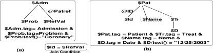
Figure 6: Join of two Tree Patterns.

Expansion: Let $t$ be a TP and $r:h_{r}\mbox{$\longleftarrow$}b_{r}$ be a mapping rule. Recall that the body $b_{r}$ consists of tree expressions possibly together with some comparison predicates (see Figure 2, e.g.). We first find a matching of $t$ to $b_{r}$, which is a substitution that maps variables in $b_{r}$ to those in $t$. This substitution (mapping) may be partial in that $b_{r}$ may contain components which have no counterpart in $t$. E.g., consider Figure 6(a). Ignore the join condition for now. Let us try to match this TP to the body of rule $1$ in Figure 2. The corresponding expansion is shown in Figure 7(a). Note that the expanded TP is just the body of rule $1$. The part of the expanded TP that was originally present in the TP (before expansion) is shown in green while the rest (i.e., the new edges coming from expansion) is shown in red (colors are represented with line styles as in the legenda). We refer to nodes that were not part of the original TP as dummy nodes. In Figure 7(a), nodes with no incident green edges are precisely the dummy nodes (e.g., $Mgh, $P, $DD, etc.).

Translation: Next, we translate the expanded TP by applying the rule to it. The correspondence between the variables in the original TP and those in the expanded TP (i.e., the rule body) is kept track of by means of a substitution between the two. Figure 7(a) shows the substitution for the TP in question as $\{\$A\mbox{$\,\rightarrow\,$}\$Adm,\$AP\mbox{$\,\rightarrow\,$}\$Prob,\$PR\mbox{$\,\rightarrow\,$}\$RefVal\}$. Using this substitution, original query constraints are propagated through the translation. In our example, the translated query resulting from applying rule $1$ to the expanded TP above is shown in Figure 7(c) (ignore the blue edge for now). For readability, all tag constraints are shown concisely by writing the tags next to the appropriate nodes. Note how the constraint $\$Prob/text()=``Coronary^{\prime\prime}$ is propagated via the substitution as $\$AP/text()=``Coronary^{\prime\prime}$. Additionally, the condition $\$PR=\$ID$ in the body of rule $1$ is used to infer that the attribute child $@ID$ of the node $\$AP/text()$ in Figure 7(c) corresponds to the attribute child $@PatRef$ of the node $\$A$ in Figure 7(a). At this point, the translated query contains Skolem functions at certain nodes. By keeping track of the correspondences between the dummy nodes in the expanded TP (Figure 7(a)) and the translated query, we can identify nodes that can be eliminated from this query. Specifically, in the expanded TP, only nodes $\$AP,\$PR$, and $$A$ were non-dummy nodes. The corresponding nodes in the translated query are $f3(\$AP/text(),\$ID,\$M,\$AD,\$DD,\$N)$ (a Skolem function whose arguments include $\$AP/text()$), and $\$ID$ (which corresponds to $\$PR$). Note that there is no counterpart for $\$A$ in Figure 7(c). So, all other nodes in the translated query are dummy nodes and can be dropped. More precisely, if a translated query node corresponds to a non-dummy node from the expanded TP or is a Skolem function one of whose arguments corresponds to non-dummy node, then it is non-dummy. Otherwise, it is dummy.

Contraction: Having identified dummy nodes in the translated query, we try to drop them. For leaf dummy nodes, this is trivial and they are always dropped, while preserving query equivalence. An internal dummy node can be dropped provided dropping it and connecting its parent and children with descendant axis (‘//’) will not change the corresponding set of DTD paths connecting them. So, whenever an internal dummy node is dropped, its parent and children are connected by a descendant edge. In Figure 7(c), all nodes with no incident green edges are dummy and can be dropped. Note that the set of paths connecting the remaining nodes remains unchanged according to the DTD $\Delta_{2}$. Each remaining (non-dummy) node is replaced with its corresponding tag. If the tag is an unconstrained variable, it is replaced by the wildcard ‘*’. If it is a constrained variable, it is replaced by each valid tag satisfying the constraint. Whenever internal dummy nodes are dropped, the corresponding child edges are replaced by descendant edges. Doing this to the translated query in Figure 7(c) yields the final contracted (shrunk) translated query in Figure 7(d). So, at this point, the final query is //Coronary/@ID.

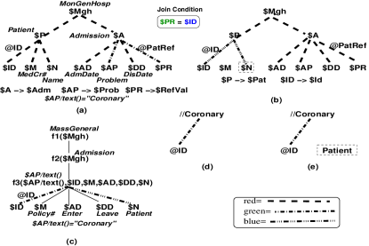
Figure 7: Translation of Join of TPs from Figure 6.

It is easy to verify that when query translation is applied to the TP in Figure 6(b), using the body of rule $1$ in Figure 2, we will get the expanded TP in Figure 7(b), the translated query in Figure 7(c) (with both green and blue edges considered), and finally the contracted translated query in Figure 7(e) (with both green and blue edges considered).

4.2.2 Translating Joins of Tree Patterns

Now, consider the query in Figure 7(a)-(b), including the join condition $\$PR=\$ID$. As illustrated above, Figure 7(a) leads to the contracted translated query //Coronary/@ID while Figure 7(b) leads to the contracted translated query //Coronary[@ID]/Name. From the join condition, we deduce that the @ID node in both queries denote the same value and hence their parent Coronary nodes must be identical. Based on this, we “stitch” the two translated queries together by identifying their Coronary nodes and their @ID nodes. So, the final contracted translated TP is isomorphic to the one shown in Figure 7(e) (with both green and blue edges considered).

4.2.3 An XQuery Example

Let us illustrate how our translation algorithm developed so far can handle a simple fragment of XQuery. This example illustrates translation in the direction of the mapping rules.

Example 1

[XQuery Forward] : Consider the XQuery query: “Find all patients with Admission/Problem = ‘Coronary’ whose Treatment started Dec, 25th 2003”, expressed as:

	Q1:	FOR $A IN //Admission,
			$P IN //Patient[@ID=$A/@PatRef]
	WHERE $A/Problem="Coronary" AND
			$P/Treat/Date="12/25/2003"
	RETURN {$P/Name}

This query can be represented as the join of two tree patterns, as shown in Figure 6(a)-(b). In the previous section, we discussed how using rule $1$ of Figure 2, this join query can be translated to the tree pattern in Figure 7(e). But that is not yet the translation of query Q1 itself: we have to consider translation via other mapping rules in Figure 2 as well. A quick inspection reveals rule $2$ is not relevant to the query as the rule heads do not contain variables corresponding to the variables in the query of Figure 6. Consider the translation via rule $3$. The expanded TP is shown in Figure 8(a). Its corresponding translated query is shown in Figure 8(b). The translation w.r.t. rule $4$ is shown in Figure 8(c) (expanded TP omitted). The contracted translated queries are shown in Figures 8(d). An important point to note is that based on the equality between $ID and $PR, the two //Progress nodes (which respectively correspond to $f2(\$ID)$ and $f2(\$PR)$, with $\$ID=\$PR$) have been merged.

Finally, in Figure 8(e), we combine the translated query obtained via rules $1$, $3$, and $4$ (see also Figure 7(e) and Figure 8(d)). The key point to notice is that since the variables $ID and $PR have been equated in the mapping rules, we can infer that the attributes @ID and @PatRef must be equal. This is again the join of two TPs and the corresponding XQuery is given in Figure 8(f).  

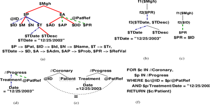
Figure 8: Translation of $Q1$ completed: tag constraints suppressed for avoiding clutter; red = solid, thick; green = dashed, thick; blue = dashed & dotted, thick.

When $Q$ is a query expressed against the DTD $\Delta_{2}$, the key intuition for query translation is to essentially follow the mapping rule in the reverse direction, i.e., from the head to the body. This has resemblances to query folding and answering queries using views [15]. However, the presence of Skolem functions greatly simplifies this process. The reason is that the node id’s act as a “glue” suggesting which subelement pieces should be associated together. Consequently, they drive exactly which mapping rule bodies we need to “join” together to rewrite the given query. We illustrate this with an example.

Example 2

[XQuery Backward] : Consider the XQuery query: “Find symptoms of patients admitted with ‘Pulmonary’ (ailment)”.

	Q2:	FOR $P IN //Progress,
			$Y IN //Pulmonary
	WHERE $Y/@ID=$P/@PatRef
	RETURN {$P/Symptom/Desc}

Figure 9 shows the join of TPs corresponding to this query. The next step is to translate each TP by matching it to each rule head. It is easy to see that only the heads of $1,2,4$ can be matched to the query (partially). The expanded TPs are obtained by matching the TPs against each of these rule heads and are shown in Figure 10(a)-(c), where to minimize clutter, we do not show tag constraints nor the substitutions between query variables and the terms in the rule heads. In essence, as for the forward direction of translation, each expanded TP is a rule head expressed as a tree expression. From the names of variables and tags the substitution between query variables and rule variables should be implicitly clear. We also mark the variables that appeared in the original query (shown via distinctly colored edges in the figure). E.g., in Figure 10(a)-(c), we know $Pulm is associated with the node $f_{3}(\$AP/text(),\$ID,\$M,\$N,\$AD,\$DD)$, $ID with the node $ID, $Prog with node $f_{2}(\$PR)$, $Symp with node $f_{3}(\$EP,\$ED)$, $Desc with node $Desc, $Prog also with the node $f_{2}(\$ID)$, and finally $PR with node $PR.

Next, each expanded TP is replaced by the tree expression in the corresponding rule body (Figure 10(d)-(f)). In doing so, we again keep track of variables mentioned in the original query. For lack of space, we give just two examples of this. Query variable $Pulm corresponds to each of the nodes labeled $AP in Figure 10(d)-(f) and query variable $Desc corresponds to the node labeled $EP in Figure 10(e). The reader should be able to work out the other correspondences with a modest effort.

The next step is to drop dummy nodes. The idea is very similar to that adopted for the forward direction of translation and is not elaborated further. Dropping of dummy nodes generates simplified but equivalent TPs. Nodes in different TPs that correspond to the same query variable are stitched together. E.g., the $A and $PR nodes in Figure 10(e) and (f) are merged. The final result of merging nodes is shown in Figure 10(g), which is actually a join of two TPs. The TPs are shown more concisely by writing the tags directly in place of the variables that are constrained by those tags. The join of TPs actually corresponds to the following XQuery statement:

	FOR $P IN //Patient,
		$A IN //Admission[@ID=$P/@ID]
	WHERE $A/Problem=’Pulmonary’
	RETURN {$P/Event}

 

Figure 9: Join of TPs corresponding to Q2.

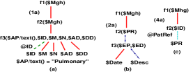
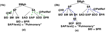
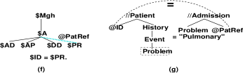
Figure 10: Steps in the Translation of Q2; red = solid, thick; green = dashed, thick; blue = dashed & dotted, thick; cyan = dashed thick.

The algorithm for query translation is given in Figure 11, and it closely follows the major steps outlined in Examples 1 and  2. Note that the algorithm shown handles one TP at a time. Handling joins of TPs follows the same general steps as discussed in the examples. We have the following result concerning the correctness of the algorithm w.r.t. query answering semantics defined in Definition 1.

Input: a tree pattern query $Q_{i}$, mapping rule set from $\Delta_{1}\rightarrow\Delta_{2}$ Output: one translated query $Q_{i}^{t}$ If $Q_{i}$ is against $\Delta_{1}$ 1.For each mapping rule $\mu_{j}$ a.Find all substitutions and expand $Q_{i}$ to $Q_{ij}^{e}$ by matching the rule body $rb_{j}$ to the query pattern $Q_{i}$ For each node $rb_{j}$ and not in $Q_{i}$, mark it as dummy If it is a distinguished node in $Q_{i}$ mark it as distinguished in the expanded query $Q_{ij}^{e}$ b.Translate each $Q_{ij}^{e}$ into $Q_{ij}^{t*}$ by applying $\mu_{j}$ Mark dummy and distinguished nodes accordingly c. Obtain contractions $Q_{ij}^{t}$ of previous translations by recursively remo- ving leaf dummy nodes and appropriate internal dummy nodes in $Q_{ij}^{t*}$ 2. Stitch together all $Q_{ij}^{t}$ to obtain resulting query $Q_{i}^{t}$. Nodes with same query variable or Skolem terms get stitched by looking at the cor- responding substitutions. Return query corresponding to $Q_{i}^{t}$ If $Q_{i}$ is against $\Delta_{2}$ 1’.For each mapping rule $\mu_{j}$ a’.Find all substitutions and expand $Q_{i}$ to $Q_{ij}^{e}$ by matching the rule head $rh_{j}$ to the query pattern $Q_{i}$ and by looking up the correspondence in the rule body $rb_{j}$ For each node in the rule head $rh_{j}$ and not in query pattern $Q_{i}$, mark it as dummy If it is a distinguished node in $Q_{i}$ mark it as distinguished in the expanded query $Q_{ij}^{e}$ b’.Translate each $Q_{ij}^{e}$ into $Q_{ij}^{t*}$ by projecting every variable of rule head $rh_{j}$ to rule body $rb_{j}$ Mark dummy and output node accordingly c’. Obtain contractions $Q_{ij}^{t}$ of previous translations by: c1) removing existential variables not appearing in $rh_{j}$ c2) recursively removing leaf dummy nodes and appropriate internal dummy nodes in $Q_{ij}^{t*}$ 2’. Stitch together nodes in all $Q_{ij}^{t}$ that correspond to the same query variable (via substitution and comparison predicates) to obtain resulting query $Q_{i}^{t}$ Return query corresponding to $Q_{i}^{t}$

Figure 11: Query Translation Algorithm

Theorem 1

[Correctness of query translation] : For the fragment of XQuery defined in Section 4.2, the query translation algorithm in Figure 11 is correct w.r.t. the semantics of query answering defined in Definition 1.  

For space reasons, we omit the proof. The proof is based on an adaptation of the well-known chase proof procedure. Before leaving this section, we note that our query translation algorithm is currently able to handle limited forms of nested XQuery expressions, as long as the query can be represented using TPs (with joins).

5 Experiments

Implementation and Setup: In this section, we examine how the query translation algorithm impacts the query performance and the scalability of HepTox. Using the mapping rules discussed in Section 3, each peer maps to a set of acquaintances. Transitive mappings produces semantic paths, and each peer is subsequently semantically connected to every other node. By means of a preliminary experiment, we realized that in order to obtain a reasonably small number of hops in network with number of peers $<=$ 128, we have to consider sets of acquaintances having at least 4 peers. Henceforth, we assume to have such sets of acquaintances for all experiments, which guarantee an average number of hops equal to 5.

Our aim is to observe how our approach behaves in a network of XML database systems having heterogeneous schemas. Hence, we derived 9 restructured variations of the XMark DTD [23], corresponding to the various transformations expressible in our mapping rule language, to produce 10 different schemas randomly scattered across the network. Detailed description of the schemas can be found on the HepToX home page [12]. We modified the XMark xmlgen code accordingly to generate the data sets corresponding to the schemas above, with sizes ranging $10MB$-$100MB$. We use Emulab [8], a network emulation testbed, to emulate a realistic P2P database. Emulab consists of a collection of PCs, whose network delay and bandwidth can be set at wish. We chose a 70ms delay and a 50MB bandwidth to simulate as much as possible the geographical networks behavior. We could get $30$ real machines for emulation. As network protocol among emulab machines, we mounted FreePastry [19], which offers a scalable and efficient P2P routing algorithm. Its O(logN) routing complexity, and O(logN) routing table size is at least as efficient as other similar projects such as CAN, Tapestry and Chord. Heptox integrates FreePastry with QIZX [22], which is apparently the fastest available open-source XQuery engine. We used FreePastry vs.1.3.2 and QIZX vs.0.4p1, respectively.

Guiding Principles: The experiments are conducted according to the following guidelines: (i) peers gets created within the Pastry network, each peer owning an independent dataset, stored in its own QIZX query engine; (ii) each peer selects other peers as its acquaintances, and these acquaintances in turn see this peer as their acquaintance; (iii) then a peer initiates a query, translates the query to the schema of each acquaintance, using our algorithm, and sends the translated query to that acquaintance; (iv) these acquaintances in turn translate the query and send it to their acquaintances, which process the query and return all the results backward to the originating peer; (v) forwarding of queries by a peer stops as soon as the peer realizes it received an already processed query request.

Scalability of HepToX: The first experiment is devoted to measuring the efficiency of the Heptox query translation algorithm (Figure 11).

Q	Query Descr.	AQTT	MQTT	ASPL
$Q_{1}$	TP with only ’/’	1180.02	2714	2.38
$Q_{2}$	TP with 1sel	749.06	1581	2.93
$Q_{3}$	TP with 1sel,1join	2057.57	4480	2.97
$Q_{4}$	TP with 2sel,1join	2236.26	4566	2.4
$Q_{5}$	TP with 2sel,1join	1749.56	3637	2.63
$Q_{6}$	TP with 2join	2054.27	4246	2.98
$Q_{7}$	TP with 1sel,2join	2299.3	4651	2.42
$Q_{8}$	TP with 1sel,1join	1379.53	3013	2.41
$Q_{9}$	TP with 2sel,2join	2472.03	4996	2.87
$Q_{10}$	TP with 2sel,3join	3172.41	7069	2.92

Table 1: AQTT (Average Query Translation Time in $ms$); MQTT (Maximum Query Translation Time in $ms$); ASPL (Average Semantic Path Length).

We derived 10 queries of increasing complexity in both structure and constraints (see brief description in Table 1, while complete queries can be be found at [12]). We broadcasted the above queries from one peer to the rest of the network (across all the acquaintances), and measured the average and maximum time taken to translate each query along all semantic paths. Table 1 shows that the translation times stay within few seconds, and increasing query complexity (e.g. query $Q_{10}$) slightly increases the translation time. In the second experiment, we aim at showing the impact of schemas heterogeneity on HepTox performance. Therefore, we vary the number of distinct heterogeneous schemas scattered around the network, and measure the average query translation time along all the semantic paths. As expected, Table 2 shows the query translation time goes from $2$ (two heterogeneous schemas across the network), to $10$ (ten heterogeneous schemas). Table 2 shows that the translation time grows linearly with the number of schemas considered and that it also depends on the complexity of the translated query. For instance, queries $Q_{6},Q_{7},Q_{9}$ and $Q_{10}$ having double joins and multiple selections, have an higher translation time.

	Nr.of Dist.Schemas
Q	2	3	4	5	6	7	8	9	10
$Q_{1}$	193	397	595	779	998	1142	1133	1194	1274
$Q_{2}$	126	231	377	505	680	844	834	872	944
$Q_{3}$	249	548	899	1187	1543	1788	1808	1909	2075
$Q_{4}$	276	576	947	1261	1629	1907	1945	2036	2155
$Q_{5}$	211	460	761	1027	1331	1557	1570	1651	1773
$Q_{6}$	327	642	1064	1381	1795	2074	2096	2209	2328
$Q_{7}$	333	658	1108	1437	1869	2189	2209	2324	2441
$Q_{8}$	212	430	705	911	1186	1376	1495	1471	1593
$Q_{9}$	308	657	1078	1440	1855	2179	2215	2340	2562
$Q_{10}$	546	973	1513	1977	2545	2975	2948	3170	3275

Table 2: Query Translation times ($ms$) with varying number of distinct schemas (obviously equal to $0$ with $1$ schema).

The next experiment wants to show the minimal overhead introduced by our translation algorithm all along the query answering process. In Figure 12(top), we measure the average time taken by each query to be completed. We highlight the various time components taken by query translation, network delay, and local query answering, respectively. It can be noted that query translation takes a negligible time if compared to network delay and local query answering. Local query answering, essentially imputable to QIZX, was the bottleneck for all queries and caused the crashing of the most complex ones. Query answers to $Q_{7}$, $Q_{9}$ and $Q_{10}$ show a cutoff point due to the fact that they never completed and were timed out. We tried different query engines before choosing QIZX, which is actually the fastest, thus this behavior was somehow outside our control.

Query Performances in HepToX: To probe the impact of our query translation algorithm on the system’s performance, we conducted an experiment in the Emulab environment in which a query is issued at an originating peer and spread across the entire network. We measured the percentage of query answers reaching the originating peer at each time interval, along with the percentage of peers completed. Figure 12(bottom) shows the results as a cumulative plot. The answers arrive in regular bursts just as expected in any normal P2P system.

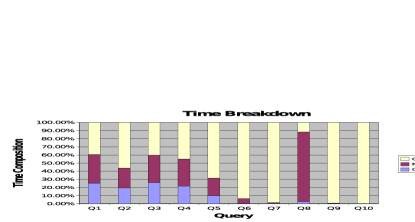
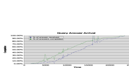
Figure 12: Query Answering Time Breakdown (top) and Time distribution of Answer Arrival at Source (bottom).

Finally, we conducted several experiments on simultaneous query processing, which is also feasible in HepTox. From these experiments, we realized that, similarly to what happens when one query is issued, the main component of time with multiple issued queries, is caused by local query answering, while the translation time still stays small. For lack of space, we omit these results.

6 Related Work

P2P data integration systems We discuss here Piazza [3, 4], Hyperion [2], Clio [20] and Lenzerini’s et al. [5]. Piazza [3, 4] defines semantic LAV/GAV-style mappings among peer schemas. Query answering semantics is based on the notion of certain answers [3], and is based on query answering using views [15], a problem not yet completely solved for XML. Our mappings are easier and more intuitive to specify, and have a data exchange semantics (similar to [2]) rather than a view semantics. Query answering also follows the same principle. In Piazza, mappings need to be provided in an XQuery-like language, while in HepTox we can infer them from diagrams. Hyperion [2] combines mapping expressions and mapping tables. Mapping tables being value-based correspondences across the world, are orthogonal to mapping expressions. Mapping tables provide a lightweight mechanism for sharing data. Our Datalog-like mapping rules follow the same direction but capture schema correspondences rather than data value ones. Clio [20, 25] also deals with XML data integration by considering semantically independent target and source nested schemas enriched with nested referential constraints. We found that this is very similar in spirit with what HepTox does. However,  [20, 25, 3, 4] are limited in the heterogeneity they deal with and do not capture the class of XML transformations involving data schema interplay (see Figure 1). Lenzerini et al. [5] address the problem of data interoperation in P2P systems using expressive schema mappings, also following the GAV/LAV paradigm, and show that the problem is in PTIME only when mapping rules are expressed in epistemic logic.

Schema-matching systems Automated techniques for schema matching (e.g. CUPID  [13], [9, 21]) are able to output elementary schema-level associations by exploiting linguistic features, context-dependent type matching, similarity functions etc. These associations could constitute the input of our rule inference algorithm if the user does not provide the arrows.

P2P systems with non-conventional lookups Popular P2P networks, e.g. Kazaa, Gnutella, advertise simple lookup queries on file names. The idea of building full-fledged P2P DBMS is being considered in many works. Internet-scale database queries and functionalities [16] as well as approximate range queries in P2P [11] and XPath queries in small communities of peers [10] have been extensively dealt with. All these works do not deal with reconciling schema heterogeneity.  [10] relies on a DHT-based network to address simple XPath queries, while [17] realizes IR-style queries in an efficient P2P relational database.

7 Conclusions and Future Work

We have presented the HepToX P2P XML database system, focusing on the following key conceptual contributions: (i) an algorithm for inferring mapping rules from correspondences between heterogeneous peer DTDs, specified via boxes and arrows; (ii) a precise and intuitive semantics for query evaluation in a P2P setting; (iii) a query translation algorithm that is correct w.r.t. this semantics and is efficient, as revealed by the detailed experimentation. We are currently investigating larger fragments of XQuery. A fundamental challenge is the reconstruction of the answers obtained from query translation in the schema of the originating peer. Another important milestone is handling 1-n and m-n correspondences between elements across DTDs in the sense of [9]. A promising recent work in this direction is [7]. It would be interesting to capture such complex mappings within our framework.

References

- [1] S. Amer-Yahia, S. Cho, L.V.S. Lakshmanan, and D. Srivastava. Minimization of Tree Pattern Queries. In SIGMOD, 2001.
- [2] M. Arenas, V. Kantere, A. Kementsietsidis, I. Kiringa, R.J. Miller, and J. Mylopoulos. The hyperion project: From data integration to data coordination. Sigmod Record, 32(3), 2003.
- [3] A.Y.Halevy, Z.G.Ives, D.Suciu, and I.Tatarinov. Schema Mediation in Peer Data Management Systems . In ICDE, 2003.
- [4] A.Y.Halevy, Z.G.Ives, P.Mork, and I.Tatarinov. Piazza: data management infrastructure for semantic web applications. In WWW, 2003.
- [5] Diego Calvanese, Giuseppe De Giacomo, Maurizio Lenzerini, and Riccardo Rosati. Logical Foundations of Peer-To-Peer Data Integration. In Proc. of ACM PODS, 2004.
- [6] Alin Deutsch and Val Tannen. Reformulation of XML Queries and Constraints. In Proc. of ICDT, 2003.
- [7] R. Dhamankar, A. Doan Y. Lee, A. Y. Halevy, and P. Domingos. iMAP: Discovering Complex Mappings between Database Schemas. In Proc. of SIGMOD, pages 383–394, 2004.
- [8] Emulab hp. http://www.emulab.net.
- [9] E.Rahm and P.A.Bernstein. A survey of approaches to automatic schema matching. VLDB J., 10(4):334–350, 2001.
- [10] L. Galanis, Y. Wang, S.R. Jeffery, and D.J. DeWitt. Locating Data Sources in Large Distributed Systems. In Proc. of VLDB, 2003.
- [11] A. Gupta, D. Agrawal, and A. El Abbadi. Approximate Range Selection Queries in Peer-to-Peer Systems. In CIDR, 2003.
- [12] HepTox. http://www.cs.ubc.ca/ laks/heptox.html.
- [13] J.Madhavan, P.A.Bernstein, and E.Rahm. Generic Schema Matching with Cupid. In Proc. of VLDB, 2001.
- [14] Anastasios Kementsietsidis, Marcelo Arenas, and Reneé J. Miller. Mapping Data in Peer-to-Peer Systems: Semantics and Algorithmic Issues. In Proc. of SIGMOD, 2003.
- [15] A. Y. Levy, A.O. Mendelzon, Y. Sagiv, and D. Srivastava. Answering Queries Using Views. In PODS, 1995.
- [16] B. T. Loo, J. M. Hellerstein, R. Huebsch, S. Shenker, and I. Stoica. Enhancing P2P File-Sharing with an Internet-Scale Query Processor. In Proc. of VLDB, 2004.
- [17] W. S. Ng, B.C. Ooi, K.L. Tan, and A.Y. Zhou. PeerDB: A P2P-based System for Distributed Data Sharing. In Proc. of ICDE, 2003.
- [18] P.A.Bernstein, F.Giunchiglia, A.Kementsietsidis, J.Mylopoulos, L.Serafini, and I.Zaihrayeu. Data Management for Peer-to-Peer Computing:A Vision. In Proc. of WebDB, 2002.
- [19] Pastry hp. http://research.microsoft.com/ antr/Pastry/.
- [20] Lucian Popa, Yannis Velegrakis, René J. Miller, Mauricio A. Hernández, and Ronald Fagin. Translating Web Data. In Proc. of VLDB, 2002.
- [21] R. Pottinger and P. A. Bernstein. Merging Models Based on Given Correspondences. In Proc. of VLDB, 2003.
- [22] Qizx. http://www.xfra.net/qizxopen/.
- [23] A. Schmidt, F. Waas, M. Kersten, M. Carey, I. Manolescu, and R. Busse. XMark: A benchmark for XML data management. In VLDB, 2002.
- [24] I. Tatarinov and A.Y. Halevy. Efficient Query Reformulation in Peer-Data Management Systems. In Proc. of SIGMOD, 2004.
- [25] Cong Yu and Lucian Popa. Constraint-Based XML Query Rewriting For Data Integration. In Proc. of SIGMOD, 2004.