Efficient Approximation of Convex Recolorings

Abstract

A coloring of a tree is convex if the vertices that pertain to any color induce a connected subtree; a partial coloring (which assigns colors to some of the vertices) is convex if it can be completed to a convex (total) coloring. Convex coloring of trees arise in areas such as phylogenetics, linguistics, etc. eg, a perfect phylogenetic tree is one in which the states of each character induce a convex coloring of the tree. Research on perfect phylogeny is usually focused on finding a tree so that few predetermined partial colorings of its vertices are convex.

When a coloring of a tree is not convex, it is desirable to know ”how far” it is from a convex one. In  [19], a natural measure for this distance, called the recoloring distance was defined: the minimal number of color changes at the vertices needed to make the coloring convex. This can be viewed as minimizing the number of “exceptional vertices” w.r.t. to a closest convex coloring. The problem was proved to be NP-hard even for colored string.
In this paper we continue the work of [19], and present a 2-approximation algorithm of convex recoloring of strings whose running time $O(cn)$, where $c$ is the number of colors and $n$ is the size of the input, and an $O(cn^{2})$-time 3-approximation algorithm for convex recoloring of trees.

1 Introduction

A phylogenetic tree is a tree which represents the course of evolution for a given set of species. The leaves of the tree are labelled with the given species. Internal vertices correspond to hypothesized, extinct species. A character is a biological attribute shared among all the species under consideration, although every species may exhibit a different character state. Mathematically, if $X$ is the set of species under consideration, a character on $X$ is a function $C$ from $X$ into a set $\cal C$ of character states. A character on a set of species can be viewed as a coloring of the species, where each color represents one of the character’s states. A natural biological constraint is that the reconstructed phylogeny have the property that each of the characters could have evolved without reverse or convergent transitions: In a reverse transition some species regains a character state of some old ancestor whilst its direct ancestor has lost this state. A convergent transition occurs if two species possess the same character state, while their least common ancestor possesses a different state.

In graph theoretic terms, the lack of reverse and convergent transitions means that the character is convex on the tree: for each state of this character, all species (extant and extinct) possessing that state induce a single block, which is a maximal monochromatic subtree. Thus, the above discussion implies that in a phylogenetic tree, each character is likely to be convex or ”almost convex”. This make convexity a fundamental property in the context of phylogenetic trees to which a lot of research has been dedicated throughout the years. The Perfect Phylogeny (PP) problem, whose complexity was extensively studied (e.g. [13, 16, 1, 17, 7, 23]), seeks for a phylogenetic tree that is simultaneously convex on each of the input characters. Maximum parsimony (MP) [10, 21] is a very popular tree reconstruction method that seeks for a tree which minimizes the parsimony score defined as the number of mutated edges summed over all characters (therefore, PP is a special case of MP). [12] introduce another criterion to estimate the distance of a phylogeny from convexity. They define the phylogenetic number as the maximum number of connected components a single state induces on the given phylogeny (obviously, phylogenetic number one corresponds to a perfect phylogeny). Convexity is a desired property in other areas of classification, beside phylogenetics. For instance, in [6, 5] a method called TNoM is used to classify genes, based on data from gene expression extracted from two types of tumor tissues. The method finds a separator on a binary vector, which minimizes the number of “1” in one side and “0” in the other, and thus defines a convex vector of minimum Hamming distance to the given binary vector. In  [14], distance from convexity is used (although not explicitly) to show strong connection between strains of Tuberculosis and their human carriers.

In a previous work  [19], we defined and studied a natural distance from a given coloring to a convex one: the recoloring distance. In the simplest, unweighted model, this distance is the minimum number of color changes at the vertices needed to make the given coloring convex (for strings this reduces to Hamming distance from a closest convex coloring). This model was extended to a weighted model, where changing the color of a vertex $v$ costs a nonnegative weight $w(v)$. The most general model studied in [19] is the non-uniform model, where the cost of coloring vertex $v$ by a color $d$ is an arbitrary nonnegative number $cost(v,d)$.

It was shown in [19] that finding the recoloring distance in the unweighted model is NP-hard even for strings (trees with two leaves), and few dynamic programming algorithms for exact solutions of few variants of the problem were presented.

In this work we present two polynomial time, constant ratio approximation algorithms, one for strings and one for trees. Both algorithms are for the weighted (uniform) model. The algorithm for strings is based on a lower bound technique which assigns penalties to colored trees. The penalties can be computed in $O(cn)$ time, and once a penalty is computed, a recoloring whose cost is smaller than the penalty is computed in linear time. The 2-approximation follows by showing that for a string, the penalty is at most twice the cost of an optimal convex recoloring. This last result does not hold for trees, where a different technique is used. The algorithm for trees is based on a recursive construction that uses a variant of the local ratio technique [3, 4], which allows adjustments of the underlying tree topology during the recursive process.

The rest of the paper is organized as follows. In the next section we present the notations and define the models used. In Section 3 we define the notion of penalty which provides lower bounds on the optimal cost of convex recoloring of any tree. In Section  4, we present the 2-approximation algorithm for the string. In Section  5 we briefly explain the local ratio technique, and present the 3-approximation algorithm for the tree. We conclude and point out future research directions in Section 6.

2 Preliminaries

A colored tree is a pair $(T,C)$ where $T=(V,E)$ is a tree with vertex set $V=\{v_{1},\ldots,v_{n}\}$, and $C$ is a coloring of $T$, i.e. - a function from $V$ onto a set of colors ${\cal C}$. For a set $U\subseteq V$, $C|_{U}$ denotes the restriction of $C$ to the vertices of $U$, and $C(U)$ denotes the set $\{C(u):u\in U\}$. For a subtree $T^{\prime}=(V(T^{\prime}),E(T^{\prime}))$ of $T$, $C(T^{\prime})$ denotes the set $C(V(T^{\prime}))$. A block in a colored tree is a maximal set of vertices which induces a monochromatic subtree. A $d$-block is a block of color $d$. The number of $d$-blocks is denoted by $n_{b}(C,d)$, or $n_{b}(d)$ when $C$ is clear from the context. A coloring $C$ is said to be convex if $n_{b}(C,d)=1$ for every color $d\in{\cal C}$. The number of $d$-violations in the coloring $C$ is $n_{b}(C,d)-1$, and the total number of violations of $C$ is $\sum_{c\in{\cal C}}(n_{b}(C,d)-1)$. Thus a coloring $C$ is convex iff the total number of violations of $C$ is zero (in [9] the above sum, taken over all characters, is used as a measure of the distance of a given phylogenetic tree from perfect phylogeny).

The definition of convex coloring is extended to partially colored trees, in which the coloring $C$ assigns colors to some subset of vertices $U\subseteq V$, which is denoted by $Domain(C)$. A partial coloring is said to be convex if it can be extended to a total convex coloring (see [22]). Convexity of partial and total coloring have simple characterization by the concept of carriers: For a subset $U$ of $V$, $carrier(U)$ is the minimal subtree that contains $U$. For a colored tree $(T,C)$ and a color $d\in C$, $carrier_{T}(C,d)$ (or $carrier(C,d)$ when $T$ is clear) is the carrier of $C^{-1}(d)$. We say that $C$ has the disjointness property if for each pair of colors $\{d,d^{\prime}\}$ it holds that $carrier(C,d)\cap carrier(C,d^{\prime})=\emptyset$. It is easy to see that a total or partial coloring $C$ is convex iff it has the disjointness property (in [8] convexity is actually defined by the disjointness property).

When some (total or partial) input coloring $(C,T)$ is given, any other coloring $C^{\prime}$ of $T$ is viewed as a recoloring of the input coloring $C$. We say that a recoloring $C^{\prime}$ of $C$ retains (the color of) a vertex $v$ if $C(v)=C^{\prime}(v)$, otherwise $C^{\prime}$ overwrites $v$. Specifically, a recoloring $C^{\prime}$ of $C$ overwrites a vertex $v$ either by changing the color of $v$, or just by uncoloring $v$. We say that $C^{\prime}$ retains (overwrites) a set of verices $U$ if it retains (overwrites resp.) every vertex in $U$. For a recoloring $C^{\prime}$ of an input coloring $C$, ${\cal X}_{C}(C^{\prime})$ (or just ${\cal X}(C^{\prime})$) is the set of the vertices overwritten by $C^{\prime}$, i.e.

$${\cal X}_{C}(C^{\prime})=\{v\in V:\left[v\in Domain(C)\right]\bigwedge\left[(v\notin Domain(C^{\prime})~{})\vee(C(v)\neq C^{\prime}(v)~{})\right]\}.$$

With each recoloring $C^{\prime}$ of $C$ we associate a cost, denoted as $cost_{C}(C^{\prime})$ (or $cost(C^{\prime})$ when $C$ is understood), which is the number of vertices overwritten by $C^{\prime}$, i.e. $cost_{C}(C^{\prime})=|{\cal X}_{C}(C^{\prime})|$. A coloring $C^{*}$ is an optimal convex recoloring of $C$, or in short an optimal recoloring of $C$, and $cost_{C}(C^{*})$ is denoted by $OPT(T,C)$, if $C^{*}$ is a convex coloring of $T$, and $cost_{C}(C^{*})\leq cost_{C}(C^{\prime})$ for any other convex coloring $C^{\prime}$ of $T$.

The above cost function naturally generalizes to the weighted version: the input is a triplet $(T,C,w)$, where $w:V\rightarrow{\mathbb{R}}^{+}\cup\{0\}$ is a weight function which assigns to each vertex $v$ a nonnegative weight $w(v)$. For a set of vertices $X$, $w(X)=\sum_{v\in X}w(v)$. The cost of a convex recoloring $C^{\prime}$ of $C$ is $cost_{C}(C^{\prime})=w({\cal X}(C^{\prime}))$, and $C^{\prime}$ is an optimal convex recoloring if it minimizes this cost.
The above unweighted and weighted cost models are uniform, in the sense that the cost of a recoloring is determined by the set of overwritten vertices, regardless the specific colors involved. [19] defines also a more subtle non uniform model, which is not studied in this paper.

Let $AL$ be an algorithm which receives as an input a weighted colored tree $(T,C,w)$ and outputs a convex recoloring of $(T,C,w)$, and let $AL(T,C,w)$ be the cost of the convex recoloring output by $AL$. We say that $AL$ is an $r$-approximation algorithm for the convex tree recoloring problem if for all inputs $(T,C,w)$ it holds that $AL(T,C,w)/OPT(T,C,w)\leq r$ [11, 15].

We complete this section with a definition and a simple observation which will be useful in the sequel. Let $(T,C)$ be a colored tree. A coloring $C^{*}$ is an expanding recoloring of $C$ if in each block of $C^{*}$ at least one vertex $v$ is retained (i.e., $C(v)=C^{*}(v)$).

Observation 2.1

let $(T=(V,E),C,w)$ be a weighted colored tree, where $w(V)>0$. Then there exists an expanding optimal convex recoloring of $C$.

Proof. Let $C^{\prime}$ be an optimal recoloring of $C$ which uses a minimum number of colors (i.e. $|C^{\prime}(V)|$ is minimized). We shall prove that $C^{\prime}$ is an expanding recoloring of $C$.

Since $w(V)>0$, the claim is trivial if $C^{\prime}$ uses just one color. So assume for contradiction that $C^{\prime}$ uses at least two colors, and that for some color $d$ used by $C^{\prime}$, there is no vertex $v$ s.t. $C(v)=C^{\prime}(v)=d$. Then there must be an edge $(u,v)$ such that $C^{\prime}(u)=d$ but $C^{\prime}(v)=d^{\prime}\neq d$. Therefore, in the uniform cost model, the coloring $C^{\prime\prime}$ which is identical to $C^{\prime}$ except that all vertices colored $d$ are now colored by $d^{\prime}$ is an optimal recoloring of $C$ which uses a smaller number of colors - a contradiction.  

In view of Observation 2.1 above, we assume in the sequel (sometimes implicitly) that the given optimal convex recolorings are expanding.

3 Lower Bounds via Penalties

In this section we present a general lower bound on the recoloring distance of weighted colored trees. Although for a general tree this bound can be fairly poor, in the next section we show that for strings it is at least half the optimal cost, and then we use this fact to obtain a 2-approximation algorithm for strings.

Let $(T,C,w)$ be a weighted colored tree. For a color $d$ and $U\subseteq V(T)$ let:

$$penalty_{C,d}(U)=w(U\cap\overline{C^{-1}(d)})+w(\overline{U}\cap{C^{-1}(d)})$$

Informally, when the vertices in $U$ induce a subtree, $penalty_{C,d}(U)$ is the total weight of the vertices which must be overwritten to make $U$ the unique $d$-block in the coloring: a vertex $v$ must be overwritten either if $v\in U$ and $C(v)\neq d$, or if $v\notin U$ and $C(v)=d$.

Figure 1: $C^{\prime}$ is a convex recoloring for $C$ which defines the following penalties: $p_{{green}}(C^{\prime})=1$, $p_{{red}}(C^{\prime})=2$, $p_{{blue}}(C^{\prime})=3$

The penalty of a given convex recoloring is sums of the penalties of every colored block: Let $C^{\prime}$ be a convex recoloring of $C$. Then:

$$penalty_{C}(C^{\prime})=\sum_{d\in{\cal C}}penalty_{C,d}(C^{{}^{\prime}-1}(d))$$

Figure 1 depicts the calculation of a penalty associated with a convex recoloring $C^{\prime}$ of $C$.

In the sequel we assume that the input colored tree $(T,C)$ is fixed, and omit it from the notations.

Claim 3.1

$penalty(C^{\prime})=2cost(C^{\prime})$

Proof. From the definitions we have

$$penalty(C^{\prime}) = \sum_{d\in{\cal C}}w\left(\{v\in V:C^{\prime}(v)=d\text{ and }C(v)\neq d\}\cup\{v\in V:C^{\prime}(v)\neq d\text{ and }C(v)=d\}\right)$$

$$= 2w(\{v\in V:C^{\prime}(v)\neq C(v)\})=2cost(C^{\prime})$$

 

As can be seen in Figure 1, $penalty(C^{\prime})=6$ while $cost(C^{\prime})=3$.

For each color $d$, $p^{*}_{d}$ is the penalty of a block which minimizes the penalty for $d$:

$$p^{*}_{d}=\min\{penalty_{d}(V(T^{\prime})):T^{\prime}\mbox{ is a subtree of }T\}$$

Corollary 3.2

For any recoloring $C^{*}$ of $C$,

$$\sum_{d\in{\cal C}}p^{*}_{d}\leq\sum_{d\in{\cal C}}penalty_{d}(C^{\prime})=2cost(C^{\prime}).$$

Proof. The inequality follows from the definition of $p^{*}_{d}$, and the equality from Claim 3.1.  

Corollary 3.2 above provides a lower bound on the cost of convex recoloring of trees. It can be shown that this lower bound can be quite poor for trees, that is: $OPT(T,C)$ can be considerably larger than $(\sum_{d\in{\cal C}}p^{*}_{d})/2$. For example, any convex recoloring of the tree in Figure 2, will recolor at least one of the big lateral blocks in the tree, while $(\sum_{d\in{\cal C}}p^{*}_{d})/2$ in that tree is the weight of the (small) central vertex (the circle). However in the next section we show that this bound can be used to obtain a polynomial time 2-approximation for convex recoloring of strings.

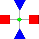
Figure 2: At least one of the lateral big blocks (triangle or rectangle) needs to be recolored.

4 A $2$-Approximation Algorithm for Strings

Let a weighted colored string $(S,C,w)$, where $S=(v_{1},\ldots,v_{n})$, be given. For $1\leq i\leq j\leq n$, $S[i,j]$ is the substring $(v_{i},v_{i+1},\ldots,v_{j})$ of $S$. The algorithm starts by finding for each $d$ a substring $B_{d}=S[i_{d},j_{d}]$ for which $penalty_{d}(S[i_{d},j_{d}])=p^{*}_{d}$. It is not hard to verify that $B_{d}$ consists of a subsequence of consecutive vertices in which the difference between the total weight of $d$-vertices and the total weight of other vertices (i.e. $w(B_{d}\cap C^{-1}(d))~{}-~{}w(B_{d}\setminus C^{-1}(d))$) is maximized, and thus $B_{d}$ can be found in linear time. We say that a vertex $v$ is covered by color $d$ if it belongs to $B_{d}$. $v$ is covered if it is covered by some color $d$, and it is free otherwise.

We describe below a linear time algorithm which, given the blocks $B_{d}$, defines a convex coloring ${\hat{C}}$ so that $cost({\hat{C}})<\sum_{d}p^{*}_{d}$, which by Corollary 3.2 is a 2-approximation to a minimal convex recoloring of $C$.

${\hat{C}}$ is constructed by performing one scan of $S$ from left to right. The scan consists of at most $c$ stages, where stage $j$ defines the $j-th$ block of ${\hat{C}}$, to be denoted $F_{j}$, and its color, $d_{j}$, as follows.

Let $d_{1}$ be the color of the leftmost covered vertex (note that $v_{1}$ is either free or covered by ${d_{1}}$). $d_{1}$ is taken to be the color of the first (leftmost) block of ${\hat{C}}$, $F_{1}$, and ${\hat{C}}(v_{1})$ is set to $d_{1}$. For $i>1$, ${\hat{C}}(v_{i})$ is determined as follows: Let $\hat{C}(v_{i-1})=d_{j}$. Then if $v_{i}\in B_{d_{j}}$ or $v_{i}$ is free, then $\hat{C}(v_{i})$ is also set to $d_{j}$. Else, $v_{i}$ must be a covered vertex. Let $d_{j+1}$ be one of the colors that cover $v_{i}$. $\hat{C}(v_{i})$ is set to $d_{j+1}$ (and $v_{i}$ is the first vertex in $F_{j+1}$).

Figure 3: The upper part of the figure shows the optimal blocks on the string and the lower part shows the coloring returned by the algorithm.

Observation 4.1

${\hat{C}}$ is a convex coloring of $S$.

Proof. Let $d_{j}$ be the color of the $j-th$ block of ${\hat{C}}$, $F_{j}$, as described above. The convexity of ${\hat{C}}$ follows from the the following invariant, which is easily proved by induction: For all $j\geq 1$, $\cup_{k=1}^{j}F_{k}\supseteq\cup_{k=1}^{j}B_{d_{k}}$. This means that, for all $j$, no vertex to the right of $F_{j}$ is covered by $d_{j}$, and hence no such vertex is colored by $d_{j}$. The observation follows.  

Thus it remains to prove

Lemma 1

$cost({\hat{C}})<\sum_{d\in{\cal C}}p^{*}_{d}$.

Proof. Let $v_{i}$ be a vertex which contributes to $cost(\hat{C})$. Then $C(v_{i})=d$ and ${\hat{C}}(v_{i})=d^{\prime}$ for some distinct $d^{\prime},d$. By the algorithm, either $v_{i}\in B_{d^{\prime}}$, or $v_{i}$ is free. In the first case $v_{i}$ contributes to both $p^{*}_{d}$ and $p^{*}_{d^{\prime}}$, and in the 2nd it contributes to $p^{*}_{d}$. The inequality is strict since in each block $F_{j}$ there is at least one vertex for which the former case holds.  

5 A 3-Approximation Algorithm for Tree

In this section we present a polynomial time algorithm which approximates the minimal convex coloring of a weighted tree by factor three. The input is a triplet $(T,C,w)$, where $w$ is a nonnegative weight function and $C$ is a (possibly partial) coloring whose domain is the set $support(w)=\{v\in V:w(v)>0\}$.

We firat introduce the notion of covers w.r.t. colored trees. A set of vertices $X$ is a convex cover (or just a cover) for a colored tree $(T,C)$ if the (partial) coloring $C_{X}=C|_{[V\setminus X]}$ is convex (i.e., $C$ can be transformed to a convex coloring by overwriting the vertices in $X$). Thus, if $C^{\prime}$ is a convex recoloring of $(T,C)$, then ${\cal X}_{C}(C^{\prime})$, the set of vertices overwritten by $C^{\prime}$, is a cover for $(T,C)$. Moreover, deciding whether a subset $X\subseteq V$ is a cover for $(T,C)$, and constructing a total convex recoloring $C^{\prime}$ of $C$ such that ${\cal X}(C^{\prime})\subseteq X$ in case it is, can be done in $O(n\cdot n_{c})$ time. Also, the cost of a recoloring $C^{\prime}$ is $w({\cal X}(C^{\prime}))$. Therefore, finding an optimal convex total recoloring of $C$ is polynomially equivalent to finding an optimal cover $X$, or equivalently a partial convex recoloring $C^{\prime}$ of $C$ so that $w({\cal X}(C^{\prime}))=w(X)$ is minimized.

Our approximation algorithm makes use of the local ratio technique, which is useful for approximating optimization covering problems such as vertex cover, dominating set, minimum spanning tree, feedback vertex set and more [4, 2, 3]. We hereafter describe it briefly:
The input to the problem is a triplet $(V,\Sigma\subseteq 2^{V},w:V\rightarrow\mathbb{R}^{+})$, and the goal is to find a subset $X\in\Sigma$ such that $w(X)$ is minimized, i.e. $w(X)=OPT(V,\Sigma,w)=\min\limits_{Y\in\Sigma}w(Y)$ (in our context $V$ is the set of vertices, and $\Sigma$ is the set of covers). The local ratio principle is based on the following observation (see e.g. [3]):

Observation 5.1

For every two weight functions $w_{1},w_{2}$:

$$OPT(V,\Sigma,w_{1})+OPT(V,\Sigma,w_{2})\leq OPT(V,\Sigma,w_{1}+w_{2})$$

Now, given our initial weight function $w$, we select $w_{1},w_{2}$ s.t. $w_{1}+w_{2}=w$ and $|supprt(w_{1})|<|support(w)|$. We first apply the algorithm to find an $r$-approximation to $(V,\Sigma,w_{1})$ (in particular, if $V\setminus support(w_{1})$ is a cover, then it is an optimal cover to $(V,\Sigma,w_{1})$). Let $X$ be the solution returned for $(V,\Sigma,w_{1})$, and assume that $w_{1}(X)\leq r\cdot OPT(V,\Sigma,w_{1})$. If we could also guarantee that $w_{2}(X)\leq r\cdot OPT(V,\Sigma,w_{2})$ then by Observation 5.1 we are guaranteed that $X$ is also an $r$-approximation for $(V,\Sigma,w_{1}+w_{2}=w)$. The original property, introduced in [4], which was used to guarantee that $w_{2}(X)\leq r\cdot OPT(V,\Sigma,w_{2})$ is that $w_{2}$ is $r$-effective, that is: for every $X\in\Sigma$ it holds that $w_{2}(X)\leq r\cdot OPT(V,\Sigma,w_{2})$ (note that if $V\in\Sigma$, the above is equivalent to requiring that $w_{2}(V)\leq r\cdot OPT(V,\Sigma,w_{2})$).

Theorem 5.2

[4] Given $X\in\Sigma$ s.t. $w_{1}(X)\leq r\cdot OPT(V,\Sigma,w_{1})$. If $w_{2}$ is $r$-effective, then $w(X)=w_{1}(X)+w_{2}(X)\leq r\cdot OPT(V,\Sigma,w)$.

We start by presenting two applications of Theorem 5.2 to obtain a $3$-approximation algorithm for convex recooloring of strings and a $4$-approximation algorithm for convex recoloring of trees.

$3$-string-APPROX: Given an instance to convex weighted string problem $(S,C,w)$: 1. If $V\setminus support(w)$ is a cover then $X\leftarrow V\smallsetminus support(w)$. Else: 2. Find 3 vertices $x,y,z\in support(w)$ s.t. $C(x)=C(z)\neq C(y)$ and $y$ lies between $x$ and $z$. (a) $\varepsilon\leftarrow\min\{w(x),w(y),w(z)\}$ (b) $w_{2}(v)=\left\{\begin{array}[]{ll}\varepsilon&\mbox{if }v\in\{x,y,z\}\\ 0&\ \mbox{otherwise.}\end{array}\right.$ (c) $w_{1}\leftarrow w-w_{2}$ (d) $X\leftarrow 3$-string-APPROX$(S,C|_{support(w_{1})},w_{1})$

Note that if a (partial) coloring of a string is not convex then the condition in 2 must hold. It is also easy to see that $w_{2}$ is $3$-effective, since any cover $Y$ must contain at least one vertex from any triplet described in condition 2, hence $w_{2}(Y)\geq\varepsilon$ while $w_{2}(V)=3\varepsilon$.

The above algorithm cannot serve for approximating convex tree coloring since in a tree the condition in 2 might not hold even if $V\setminus support(w)$ is not a cover. In the following algorithm we generalize this condition to one which must hold in any non-convex coloring of a tree, in the price of increasing the approximation ratio from 3 to 4.

$4$-tree-APPROX: Given an instance to convex weighted tree problem $(T,C,w)$: 1. If $V\smallsetminus support(w)$ is a cover then $X\leftarrow V\smallsetminus support(w)$. Else: 2. Find two pairs of (not necessarily distinct) vertices $(x_{1},x_{2})$ and $(y_{1},y_{2})$ in $support(w)$ s.t. $C(x_{1})=C(x_{2})\neq(y_{1})=C(y_{2})$, and $carrier(\{x_{1},x_{2}\})\cap carrier(\{y_{1},y_{2}\})\neq\emptyset$: (a) $\varepsilon\leftarrow\min\{w(x_{i}),w(y_{i})\}$, $i=\{1,2\}$ (b) $w_{2}(v)=\left\{\begin{array}[]{ll}\varepsilon&\mbox{if }v\in\{x_{1},x_{2},y_{1},y_{2}\}\\ 0&\ \mbox{otherwise.}\end{array}\right.$ (c) $w_{1}\leftarrow w-w_{2}$ (d) $X\leftarrow 4$-tree-APPROX$(S,C|_{support(w_{1})},w_{1})$

The algorithm is correct since if there are no two pairs as described in step 2, then $V\setminus support(w)$ is a cover. Also, it is easy to see that $w_{2}$ is 4-effective. Hence the above algorithm returns a cover with weight at most $4\cdot OPT(T,C,w)$.

We now describe algorithm $3$-tree-APPROX. Informally, the algorithm uses an iterative method, in the spirit of the local ratio technique, which approximates the solution of the input $(T,C,w)$ by reducing it to $(T^{\prime},C^{\prime},w_{1})$ where $|support(w_{1})|<|support(w)|$. Depending on the given input, this reduction is either of the local ratio type (via an appropriate $3$-effective weight function) or, the input graph is replaced by a smaller one which preserves the optimal solutions.

$3$-tree-APPROX$(T,C,w)$ On input $(T,C,w)$ of a weighted colored tree, do the following: 1. If $V\setminus support(w)$ is a cover then $X\leftarrow V\smallsetminus support(w)$. Else: 2. $(T^{\prime},C^{\prime},w_{1})\leftarrow REDUCE(T,C,w)$. $\setminus$The function $REDUCE$ guarantees that $|support(w_{1})|<|support(w)|$ (a) $X^{\prime}\leftarrow$ $3$-tree-APPROX$(T^{\prime},C^{\prime},w_{1})$. (b) $X\leftarrow UPDATE(X^{\prime},T)$. $\setminus$The function $UPDATE$ guarantees that if $X^{\prime}$ is a 3-approximation to $(T^{\prime},C^{\prime},w_{1})$, then $X$ is a 3-approximation to $(T,C,w)$.

Next we describe the functions $REDUCE$ and $UPDATE$, by considering few cases. In the first two cases we employ the local ratio technique.

Case 1: $support(w)$ contains three vertices $x,y,z$ such that $y$ lies on the path from $x$ to $z$ and $C(x)=C(z)\neq C(y)$.
In this case we use the same reduction of $3$-string-APPROX: Let $\varepsilon=\min\{w(x),w(y),w(z)\}>0$. Then $REDUCE(T,C,w)=(T,C|_{support(w_{1})},w_{1})$, where $w_{1}(v)=w(v)$ if $v\notin\{x,y,z\}$, else $w_{1}(v)=w(v)-\varepsilon$. The same arguments which implies the correctness of $3$-string-APPROX implies that if $X^{\prime}$ is a 3-approximation for $(T^{\prime},C^{\prime},w_{1})$, then it is also a 3-approximation for $(T,C,w)$, thus we set $UPDATE(X^{\prime},T)=X^{\prime}$.

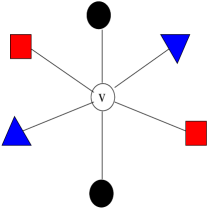
Figure 4: Case 2: a vertex $v$ is contained in 3 different carriers.

Case 2: Not Case 1, and $T$ contains a vertex $v$ such that $v\in\cap_{i=1}^{3}carrier(d_{i},C)$ for three distinct colors $d_{1},d_{2}$ and $d_{3}$ (see Figure 4).
In this case we must have that $w(v)=0$ (else Case 1 would hold), and there are three designated pairs of vertices $\{x_{1},x_{2}\},\{y_{1},y_{2}\}$ and $\{z_{1},z_{2}\}$ such that $C(x_{i})=d_{1}$, $C(y_{i})=d_{2},C(z_{i})=d_{3}(i=1,2)$, and $v$ lies on each of the three paths connecting these three pairs (see Figure 4). We set $REDUCE(T,C,w)=(T,C|_{support(w_{1})},w_{1})$, where $w_{1}$ is defined as follows.
Let $\varepsilon=\min\{w(x_{i}),w(y_{i}),w(z_{i}):i=1,2\}$. Then $w_{1}(v)=w(v)$ if $v$ is not in one of the designated pairs, else $w_{1}(v)=w(v)-\varepsilon$. Finally, any cover for $(T,C)$ must contain at least two vertices from the set $\{x_{i},y_{i},z_{i}:i=1,2\}$, hence $w-w_{1}=w_{2}$ is 3-effective, and by the local ratio theorem we can set $UPDATE(X^{\prime},T)=X^{\prime}$.

Case 3: Not Cases 1 and 2.
Root $T$ at some vertex $r$ and for each color $d$ let $r_{d}$ be the root of the subtree $carrier(d,C)$. Let $d_{0}$ be a color for which the root ${r_{d_{0}}}$ is farthest from $r$. Let ${\bar{T}}$ be the subtree of $T$ rooted at $r_{d_{0}}$, and let $\hat{T}=T\setminus{\bar{T}}$ (see Figure 5). By the definition of ${r_{d_{0}}}$, no vertex in $\hat{T}$ is colored by $d_{0}$, and since Case 2 does not hold, there is a color $d^{\prime}$ so that $\{d_{0}\}\subseteq C(V({\bar{T}}))\subseteq\{d_{0},d^{\prime}\}$.

Figure 5: Case 3: Not case 1 nor 2. $\bar{T}$ is the subtree rooted at ${r_{d_{0}}}$ and $\hat{T}=T\setminus{\bar{T}}$.

Subcase 3a: $C(V({\bar{T}}))=\{d_{0}\}$ (see Figure 6).
In this case, $carrier(d_{0},C)\cap carrier(d,C)=\emptyset$ for each color $d\neq d_{0}$, and for each optimal solution $X$ it holds that $X\cap V({\bar{T}})=\emptyset$. We set $REDUCE(T,C,w)\leftarrow(\hat{T},C|_{V(\hat{T})},w|_{V(\hat{T})})$. The 3-approximation $X^{\prime}$ to $(T^{\prime},C^{\prime},w_{1})$ is also a 3-approximation to $(X,C,w)$, thus $UPDATE(X^{\prime},T)=X^{\prime}$.

Figure 6: Case 3a: No vertices of $\hat{T}$ are colored by $d^{\prime}$.

We are left with the last case.
Subcase 3b: ${r_{d_{0}}}\in carrier(d_{0},C)\cap carrier(d^{\prime},C)$. See Figure 7.
Observe that in this case we have $w({r_{d_{0}}})=0$ and $|support(w)\cap V({\bar{T}})|\geq 3$, since $V({\bar{T}})$ must contain at least two vertices colored $d_{0}$ and at least one vertex colored $d^{\prime}$. Figure 7 illustrates this case.

Figure 7: Case 3b: ${r_{d_{0}}}\in T_{d_{0}}\cap carrier(d^{\prime})$

Observation 5.3

There is an optimal convex coloring $C^{\prime}$ which satisfies the following: $C^{\prime}(v)\neq d_{0}$ for any $v\in V(\hat{T})$, and $C^{\prime}(v)\in\{d_{0},d^{\prime}\}$ for any $v\in V({\bar{T}})$.

Proof. Let ${\hat{C}}$ be an expanding optimal convex recoloring of $(T,C)$. We will show that there is an optimal coloring $C^{\prime}$ satisfying the lemma such that $cost(C^{\prime})\leq cost({\hat{C}})$. Since ${\hat{C}}$ is expanding and optimal, at least one vertex in ${\bar{T}}$ is colored either by $d_{0}$ or by $d^{\prime}$. Let $U$ be a set of vertices in ${\bar{T}}$ so that $carrier(U)$ is a maximal subtree all of whose vertices are colored by colors not in $\{d_{0},d^{\prime}\}$. Then $carrier(U)$ must have a neighbor $u$ in ${\bar{T}}$ s.t. ${\hat{C}}(u)\in\{d_{0},d^{\prime}\}$. Change the colors of the vertices in $U$ to ${\hat{C}}(u)$. This procedure can be repeated until all the vertices of ${\bar{T}}$ are colored by $d_{0}$ or by $d^{\prime}$, without increasing the cost of the recoloring. A similar procedure can be used to change the color of all the verticed in $\hat{T}$ to be different from $d_{0}$. It is easy to see that the resulting coloring $C^{\prime}$ is convex and $cost(C^{\prime})\leq cost({\hat{C}})$.  

The function $REDUCE$ in Subcase 3b is based on the following observation: Let $C^{\prime}$ be any optimal recoloring of $T$ satisfying Observation 5.3, and let $s$ be the parent of ${r_{d_{0}}}$ in $T$. Then $C^{\prime}|_{V({\bar{T}})}$, the restriction of the coloring $C^{\prime}$ to the vertices of ${\bar{T}}$, depends only on whether $carrier(d^{\prime},C^{\prime})$ intersects ${V(\hat{T})}$, and in this case if it contains the vertex $s$. Specifically, $C^{\prime}_{V({\bar{T}})}$ must be one of the three colorings of $V({\bar{T}})$, $C_{high},C_{medium}$ and $C_{min}$, according to the following three scenarios:

1. $carrier(d^{\prime},C^{\prime})\cap V(\hat{T})\neq\emptyset$ and $s\notin carrier(d^{\prime},C^{\prime})$. Then it must be the case that $C^{\prime}$ colors all the vertices in $V({\bar{T}})$ by $d_{0}$. This coloring of ${\bar{T}}$ is denoted as $C_{high}$.

2. $carrier(d^{\prime},C^{\prime})\cap V(\hat{T})\neq\emptyset$ and $s\in carrier(d^{\prime},C^{\prime})$. Then $C^{\prime}|_{{\bar{T}}}$ is a coloring of minimal possible cost of ${\bar{T}}$ which either equals $C_{high}$ (i.e. colors all vertices by $d_{0}$), or otherwise colors ${r_{d_{0}}}$ by $d^{\prime}$. This coloring of ${\bar{T}}$ is called $C_{medium}$.

3. $carrier(d^{\prime},C^{\prime})\cap V(\hat{T})=\emptyset$. Then $C^{\prime}|_{{\bar{T}}}$ must be an optimal convex recoloring of ${\bar{T}}$ by the two colors $d_{0},d^{\prime}$. This coloring of ${\bar{T}}$ is called $C_{min}$.

We will show soon that the colorings $C_{high},C_{medium}$ and $C_{min}$ above can be computed in linear time. The function $REDUCE$ in Subcase 3b modifies the tree $T$ by replacing ${\bar{T}}$ by a subtree ${\bar{T_{0}}}$ with only 2 vertices, ${r_{d_{0}}}$ and $v_{0}$, which encodes the three colorings $C_{high},C_{medium},C_{min}$. Specifically, $REDUCE(T,C,w)=(T^{\prime},C^{\prime},w_{1})$ where (see Figure 8):

• $T^{\prime}$ is obtained from $T$ by replacing the subtree ${\bar{T}}$ by the subtree ${\bar{T_{0}}}$ which contains two vertices: a root ${r_{d_{0}}}$ with a single descendant $v_{0}$.

• $w_{1}(v)=w(v)$ for each $v\in V(\hat{T})$. For ${r_{d_{0}}}$ and $v_{0}$, $w_{1}$ is defined as follows: $w_{1}({r_{d_{0}}})=cost(C_{medium})-cost(C_{min})$ and $w_{1}(v_{0})=cost(C_{high})-cost(C_{min})$.

• $C^{\prime}(v)=C(v)$ for each $v\in V(\hat{T})$; If $w({r_{d_{0}}})>0)$ then $C^{\prime}({r_{d_{0}}})=d_{0}$ and if $w(v_{0})>0$ then $C^{\prime}(v_{0})=d^{\prime}$. (If $w_{1}(u)=0$ for $u\in\{{r_{d_{0}}},v_{0}\}$, then $C^{\prime}(u)$ is undefined).

Figure 8 illustrates $REDUCE$ for case 3b. In the figure, $C_{high}$ requires overwriting all $d^{\prime}$ vertices and therefore costs $3$, $C_{medium}$ requires overwriting one $d_{0}$ vertex and costs $2$ and $C_{min}$ is the optimal coloring for ${\bar{T}}$ with cost $1$. The new subtree ${\bar{T_{0}}}$ reflects these weight with $w_{1}(r_{d_{0}})=C_{medium}-C_{min}=1$ and $w_{1}(v_{0})=C_{high}-C_{min}=2$.

Figure 8: $REDUCE$ of case 3b: ${\bar{T}}$ is replaced with ${\bar{T_{0}}}$ where $w_{1}(r_{d_{0}})=C_{medium}-C_{min}=1$ and $w_{1}(v_{0})=C_{high}-C_{min}=2$.

Claim 5.4

$OPT(T^{\prime},C^{\prime},w_{1})=OPT(T,C,w)-cost(C_{min})$.

Proof. We first show that $OPT(T^{\prime},C^{\prime},w_{1})\leq OPT(T,C,w)-cost(C_{min})$. Let $C^{*}$ be an optimal recoloring of $C$ satisfying Observation 5.3, and let $X^{*}={\cal X}(C^{*})$. By the discussion above, we may assume that $C^{*}|_{V({\bar{T}})}$ has one of the forms $C_{high},C_{medium}$ or $C_{min}$. Thus, $X^{*}\cap{V({\bar{T}})}$ is either ${\cal X}(C_{high}),{\cal X}(C_{medium})$ or ${\cal X}(C_{min})$. We map $C^{*}$ to a coloring $C^{\prime}$ of $T^{\prime}$ as follows: for $v\in\ V(\hat{T})$, $C^{\prime}(v)=C^{*}(v)$. $C^{\prime}$ on ${r_{d_{0}}}$ and $v_{0}$ is defined as follows:

• If $C^{*}|_{V({\bar{T}})}=C_{high}$ then $C^{\prime}({r_{d_{0}}})=C^{\prime}(v_{0})=d_{0}$, and $cost(C^{\prime}|_{V({\bar{T}}})=w_{1}(v_{0})$;

• If $C^{*}|_{V({\bar{T}})}=C_{medium}$ then $C^{\prime}({r_{d_{0}}})=C^{\prime}(v_{0})=d^{\prime}$, and $cost(C^{\prime}|_{V({\bar{T}}})=w_{1}({r_{d_{0}}})$;

• If $C^{*}|_{V({\bar{T}})}=C_{min}$ then $C^{\prime}({r_{d_{0}}})=d_{0}$, $C^{\prime}(v_{0})=d^{\prime}$, and $cost(C^{\prime}|_{V({\bar{T}}})=0$.

Note that in all three cases, $cost(C^{\prime})=cost(C^{*})-cost(C_{min})$.

The proof of the opposite inequality $OPT(T,C,w)-cost(C_{min})\leq OPT(T^{\prime},C^{\prime},w_{1})$ is similar.  

Corollary 5.5

$C^{*}$ is optimal recoloring of $(T,C,w)$ iff $C^{\prime}$ is an optimal recoloring of $(T^{\prime},C^{\prime},w_{1})$.

We now can define the $UPDATE$ function for Subcase 3b: Let $X^{\prime}=$3$-tree-APPROX(T^{\prime},C^{\prime},w_{1})$. Then $X^{\prime}$ is a disjoint union of the sets $\hat{X^{\prime}}=X^{\prime}\cap V(\hat{T})$ and ${\bar{X^{\prime}}_{0}}=X^{\prime}\cap V({\bar{T_{0}}})$. Moreover, ${\bar{X^{\prime}}_{0}}\in\{\{{r_{d_{0}}}\},\{v_{0}\},\emptyset\}$. Then $X\leftarrow UPDATE(X^{\prime})=\hat{X^{\prime}}\cup{\bar{X^{\prime}}}$, where ${\bar{X^{\prime}}}$ is ${\cal X}(C_{high})$ if ${\bar{X^{\prime}}_{0}}=\{{r_{d_{0}}}\}$, is ${\cal X}(C_{medium})$ if ${\bar{X^{\prime}}_{0}}=\{v_{0}\}$, and is ${\cal X}(C_{min})$ if ${\bar{X^{\prime}}_{0}}=\emptyset$. Note that $w(X)=w(X^{\prime})+cost(C_{min})$. The following inequalities show that if $w_{1}(X^{\prime})$ is a 3-approximation to $OPT(T^{\prime},C^{\prime},w_{1})$, then $w(X)$ is a 3-approximation to $OPT(T,C,w)$:

$$w(X) = w_{1}(X^{\prime})+cost(C_{min})\leq 3OPT(T^{\prime},C^{\prime},w_{1})+cost(C_{min})$$

$$< 3(OPT(T^{\prime},C^{\prime},w_{1})+cost(C_{min}))=3OPT(T,C,w)$$

5.1 A Linear Time Algorithm for Subcase 3b

In subcase 3b we need to compute $C_{high}$, $C_{medium}$ and $C_{min}$. The computation of $C_{high}$ is immediate. $C_{medium}$ and $C_{min}$ can be computed by the following simple, linear time algorithm that finds a minimal cost convex recoloring of a bi-colored tree, under the constraint that the color of a given vertex $r$ is predetermined to one of the two colors.
Let the weighted colored tree $(T,C,w)$ and the vertex $r$ be given, and let $\{d_{1},d_{2}\}=C(T)$. For $i\in\{1,2\}$, let $C_{i}$ the minimal cost convex recoloring which sets the color of $r$ to $d_{i}$ (note that a coloring with minimum cost in $\{C_{1},C_{2}\}$ is an optimal convex recoloring of $(T,C)$). We illustrate the computation of $C_{1}$ (the computation of $C_{2}$ is similar):
Compute for every edge $e=(u\rightarrow v)$ a cost defined by

$$cost(e)=\displaystyle w(\{v^{\prime}:v^{\prime}\in T(v)\text{ and }C(v^{\prime})=d_{1}\})+\displaystyle w(\{v^{\prime}:v^{\prime}\in[T\setminus T(v)]\text{ and }C(v^{\prime})=d_{2}\})$$

where $T(v)$ is the subtree rooted at $v$. This can be done by one post order traversal of the tree. Then, select the edge $e^{*}=(u_{0}\rightarrow v_{0})$ which minimizes this cost, and set $C_{1}(w)=d_{2}$ for each $w\in T(v_{0})$, and $C_{1}(w)=d_{1}$ otherwise.

5.2 Correctness and complexity

We now summarize the discussion of the previous section to show that the algorithm terminates and return a cover $X$ which is a 3-approximation for $(T,C,w)$.

Let $(T=(V,E),C,w)$ be an input to $3$-tree-APPROX. if $V\setminus support(w)$ is a cover then the returned solution is optimal. Else, in each of the cases, $REDUCE(T,C,w)$ reduces the input to $(T^{\prime},C^{\prime},w_{1})$ such that $|support(w_{1})|<|support(w)|$, hence the algorithm terminates within at most $n=|V|$ iterations. Also, as detailed in the previous subsections, the function $UPDATE$ guarantees that that if $X^{\prime}$ is a 3-approximation for $(T^{\prime},C^{\prime},w_{1})$ then $X$ is a 3-approximation to $(T,C,w)$. Thus after at most $n$ iterations the algorithm provides a 3-approximation to the original input.

Checking whether Case 1, Case 2, Subcase 3a or Subcase 3b holds at each stage requires $O(cn)$ time for each of the cases, and computing the function $REDUCE$ after the relevant case is identified requires linear time in all cases. Since there are at most $n$ iterations, the overall complexity is $O(cn^{2})$. Thus we have

Theorem 5.6

Algorithm $3$-tree-APPROX  is a polynomial time 3-approximation algorithm for the minimum convex recoloring problem.

6 Discussion and Future Work

In this work we showed two approximation algorithms for colored strings and trees, respectively. The 2-approximation algorithm relies on the technique of penalizing a colored string and the 3-approximation algorithm for the tree extends the local ratio technique by allowing dynamic changes in the underlying graph.

Few interesting research directions which suggest themselves are:

• Can our approximation ratios for strings or trees be improved.

• This is a more focused variant of the previous item. A problem has a polynomial approximation scheme [11, 15], or is fully approximable [20], if for each $\varepsilon$ it can be $\varepsilon$-approximated in $p_{\varepsilon}(n)$ time for some polynomial $p_{\varepsilon}$. Are the problems of optimal convex recoloring of trees or strings fully approximable, (or equivalently have a polynomial approximation scheme)?

• Alternatively, can any of the variant be shown to be APX-hard ?

• The algorithms presented here apply only to uniform models. The non uniform model, motivated by weighted maximum parsimony [21], assumes that the cost of assigning color $d$ to vertex $v$ is given by an arbitrary nonnegative number $cost(v,d)$ (note that, formally, no initial coloring $C$ is assumed in this cost model). In this model $cost(C^{\prime})$ is defined only for a total recoloring $C^{\prime}$, and is given by the sum $\sum_{v\in V}cost(v,C^{\prime}(v))$. Finding non-trivial approximation results for this model is challanging.

7 Acknowledgments

We wish to thank Reuven Bar Yehuda and Mike Steel for many helpful discussions.

References

- [1] R. Agrawala and D. Fernandez-Baca. Simple algorithms for perfect phylogeny and triangulating colored graphs. International Journal of Foundations of Computer Science, 7(1):11–21, 1996.
- [2] V. Bafna, P. Berman, and T. Fujito. A 2-approximation algorithm for the undirected feedback vertex set problem. SIAM J. on Discrete Mathematics, 12:289–297, 1999.
- [3] R. Bar-Yehuda. One for the price of two: A unified approach for approximating covering problems. Algorithmica, 27:131–144, 2000.
- [4] R. Bar-Yehuda and S. Even. A local-ratio theorem for approximating the weighted vertex cover problem. Annals of Discrete Mathematics, 25:27–46, 1985.
- [5] A. Ben-Dor, N. Friedman, and Z. Yakhini. Class discovery in gene expression data. In RECOMB, pages 31–38, 2001.
- [6] M. Bittner and et.al. Molecular classification of cutaneous malignant melanoma by gene expression profiling. Nature, 406(6795):536–40, 2000.
- [7] H.L. Bodlaender, M.R. Fellows, and T. Warnow. Two strikes against perfect phylogeny. In ICALP, pages 273–283, 1992.
- [8] A. Dress and M.A. Steel. Convex tree realizations of partitions. Applied Mathematics Letters,, 5(3):3–6, 1992.
- [9] D. Fern ndez-Baca and J. Lagergren. A polynomial-time algorithm for near-perfect phylogeny. SIAM Journal on Computing, 32(5):1115–1127, 2003.
- [10] W. M. Fitch. A non-sequential method for constructing trees and hierarchical classifications. Journal of Molecular Evolution, 18(1):30–37, 1981.
- [11] M. R. Garey and D. S. Johnson. Computers and Intractability; A Guide to the Theory of NP-Completeness. W.H. Freeman and Company, 1979.
- [12] L.A. Goldberg, P.W. Goldberg, C.A. Phillips, Z Sweedyk, and T. Warnow. Minimizing phylogenetic number to find good evolutionary trees. Discrete Applied Mathematics, 71:111–136, 1996.
- [13] D. Gusfield. Efficient algorithms for inferring evolutionary history. Networks, 21:19–28, 1991.
- [14] A. Hirsh, A. Tsolaki, K. DeRiemer, M. Feldman, and P. Small. From the cover: Stable association between strains of mycobacterium tuberculosis and their human host populations. PNAS, 101:4871–4876, 2004.
- [15] D. S. Hochbaum, editor. Approximation Algorithms for NP-Hard Problem. PWS Publishing Company, 1997.
- [16] S. Kannan and T. Warnow. Inferring evolutionary history from DNA sequences. SIAM J. Computing, 23(3):713–737, 1994.
- [17] S. Kannan and T. Warnow. A fast algorithm for the computation and enumeration of perfect phylogenies when the number of character states is fixed. SIAM J. Computing, 26(6):1749–1763, 1997.
- [18] S. Moran and S. Snir. Convex recoloring of strings and trees. Technical Report CS-2003-13, Technion, November 2003.
- [19] S. Moran and S. Snir. Convex recoloring of strings and trees: Definitions, hardness results and algorithms. submitted, 2004.
- [20] A. Paz and S. Moran. Non deterministic polynomial optimization probems and their approximabilty. Theoretical Computer Science, 15:251–277, 1981. Abridged version: Proc. of the 4th ICALP conference, 1977.
- [21] D. Sankoff. Minimal mutation trees of sequences. SIAM Journal on Applied Mathematics, 28:35–42, 1975.
- [22] C. Semple and M.A. Steel. Phylogenetics. Oxford University Press, 2003.
- [23] M. Steel. The complexity of reconstructing trees from qualitative characters and subtrees. Journal of Classification, 9(1):91–116, 1992.
- [24] V. Vazirani. Approximation Algorithms. Springer, Berlin, germany, 2001.