Instance-Independent View Serializability for Semistructured Databases
Abstract
Semistructured databases require tailor-made concurrency control mechanisms since traditional solutions for the relational model have been shown to be inadequate. Such mechanisms need to take full advantage of the hierarchical structure of semistructured data, for instance allowing concurrent updates of subtrees of, or even individual elements in, XML documents. We present an approach for concurrency control which is document-independent in the sense that two schedules of semistructured transactions are considered equivalent if they are equivalent on all possible documents. We prove that it is decidable in polynomial time whether two given schedules in this framework are equivalent. This also solves the view serializability for semistructured schedules polynomially in the size of the schedule and exponentially in the number of transactions.
1 Introduction
In previous work [5, 6, 7] we have shown that traditional concurrency control [21] mechanisms for the relational model [2, 11, 19, 20] are inadequate to capture the complicated update behavior that is possible for semistructured databases. Indeed, when XML documents are stored in relational databases, their hierarchical structure becomes invisible to the locking strategy used by the database management system.
In general two actions, on two different nodes of a document tree, that are completely ‘independent’ from each other, cannot cause a conflict, even if they are updates. Changing the spelling of the name of one of the authors of a book and adding a chapter to the book cannot cause a conflict for instance. Most classical concurrency control mechanisms, when applied in a naive way to semistructured data, will not allow such concurrent updates. This consideration is the main reason why the classical approaches seem to be inadequate as a concurrency control mechanism for semistructured data.
Most of the work on concurrency control for XML and semistructured data is based on the observation that the data is usually accessed by means of XPath expressions. Therefore it is suggested in [5] to use a simplified form of XPath expressions as locks on the document such that precisely all operations that change the result of the expression are no longer allowed. Two alternatives for conflict-checking are proposed, one where path locks are propagated down the XML tree and one where updates are propagated up the tree, which both have their specific benefits. This approach is extended in [7] where a commit-scheduler is defined and it is proved that the schedules it generates are serializable. Finally in [9] an alternative conflict-scheduler is introduced that allows more schedules than the previously introduced commit-scheduler.
A similar approach is taken in [4] where conflicts with path locks are detected by accumulating updates in the XML tree and intelligently recomputing the results of the path expressions. As a result they can allow more complex path expressions, but conflict checking becomes more expensive. Another related approach is presented in [17] where locks are derived from the path expressions and a protocol for these locks is introduced that guarantees serializability.
Several locking protocols that are not based on path expressions but on DOM operations are introduced in [14, 15]. Here, there are locks that lock the whole document, locks that lock all the children of a certain node and locks that lock individual nodes or pointers between them. An interesting new aspect is here the possibility to use the DTD for conflict reduction and thus allowing more parallelism. Although these locking protocols seem very suitable in the case of DOM operations, it is not clear whether they will also perform well if most of the access is done by path expressions. A similar approach, but extended with the aspect of multi-granularity locking, is presented in [12, 13]. This approach seems more suitable for hierarchical data like semistructured data and XML. However, such mechanisms will often allow less concurrency than a path based locking protocol would.
A potential problem with many of the previously mentioned protocols is that locks are associated with document nodes and so for large documents we may have large numbers of locks. A possible solution for this is presented in [10] where the locks are associated with the nodes in a DataGuide, which is usually much smaller than the document. However, this protocol does not guarantee serializability and allows phantoms.
For all the approaches above it holds that the concurrency control mechanisms are somehow dependent upon the document. In most cases this means that if the document gets very large then the overhead may also become very large. This paper investigates the possibilities of a document-independent concurrency control mechanism. It extends the preliminary results on this subject that were presented in [8].
The total behavior of the processes that we consider in this paper is straightforward: each cooperating process produces a transaction of atomic actions that are queries or updates on the actual document. The transactions are interleaved by the scheduler and the resulting schedule has to be equivalent with a serial schedule. Two schedules on the same set of transactions are called equivalent iff for each possible input document they represent the same transformation and each query gives the same result in both schedules. This is a special definition of view equivalency, which we will use to decide view serializability [3] for a schedule.
Note that we consider view serializability, as opposed to conflict serializability. As we will show later on, conflict serializability, which might be more interesting from a computational point of view, will allow less schedules to be serialized and hence can be too restrictive.
The updates that we consider are very primitive: the addition of an edge of the document tree and the deletion of an edge. Semantically the addition is only defined if the added edge does not already exist in the document tree. Analogously the deletion is only defined if the deleted edge exists. A more general semantics, that does not include this constraint, can be easily simulated by adding first some queries.
There are some schedules for which the result is undefined for all document trees (e.g., a schedule consisting of two consecutive deletions of the same edge). These schedules are meaningless and are called inconsistent. Hence a schedule is consistent if there exists at least one document tree on which its application is defined. We prove that the consistenty of schedules is polynomially decidable.
In order to tackle the equivalence of schedules and transactions we first consider schedules without queries, and as such we have only to focus on the transformational behavior of the schedules. We will see that, contrary to the relational model, the swapping of the actions cannot help us in detecting the equivalence of two schedules. We prove that the equivalence of queryless schedules is also polynomially decidable, and that view serializability is exponentially decidable in the number of transactions and polynomially in the number of operations. Finally we generalize the results above for general schedules over the same set of transactions.
The paper contains a number of theoretical results on which the algorithms are based. The algorithms are a straightforward consequence of the given proofs or sketches. The complete proofs are given in [16].
The paper is structured as follows: Section 2 defines the data model, the operations and the semistructured schedules. Section 3 studies the consistency of schedules without queries. In Section 4 we study the equivalence and the view serializability problem for these queryless schedules. In Section 5 we generalize these results for consistent schedules.
2 Data Model and Operations
The data model we use is derived from the classical data model for semistructured data [1]. We consider directed, unordered trees in which the edges are labelled.
Consider a fixed universal set of nodes and a fixed universal set of edge labels not containing the symbol .
Definition 1.
A graph is a tuple with and . A document tree (dt) is a tuple such that is a graph that represents a tree with root . The edges are directed from the parent to the child.
Example 1.
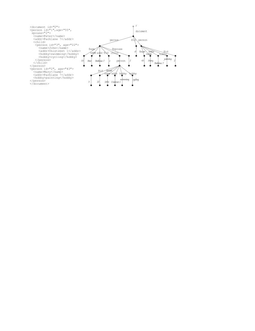
Figure 1 shows a fragment of an XML document and its dt representation.
This data model closely mimics the XML data model as illustrated in the next example. We remark, however, the following differences:
-
•
order: Siblings are not ordered. This is not crucial, as an ordering can be simulated by using a skewed binary dt.
-
•
attributes: Attributes, like elements, are represented by edges labeled by the name of the attributes (started with a @). The difference is that in this data model an element may contain several attributes of the same name.
-
•
labels: Labels represent not only tag names and attribute names, but also values and text.
-
•
text: Unlike in XML, it is possible for several text edges to be adjacent to each other.
A label path is a string of the form with and every an edge label in . Given a path in a graph , the label path of , denoted (or when is subsumed) is the string .
Processes working on document trees do so in the context of a general programming language that includes an interface to a document server which manages transactions on documents. The process generates a list of operations that will access the document. In general there are three types of operations: the query, the addition and the deletion. The input to a query operation will be a node and a simple type of path expression, while the result of the invocation of a query operation will be a set of nodes. The programming language includes the concepts of sets, and has constructs to iterate over their entire contents. The input to an addition or a deletion will be an edge. The result of an addition or a deletion will be a simple transformation of the original tree into a new tree. If the result would not be a tree anymore it is not defined.
We now define the path expressions and the query operations, subsuming a given dt .
The syntax of path expressions111Remark that path expressions form a subset of XPath expressions. is given by :
The set of label paths represented by a path expression is defined as follows:
Let be an arbitrary node of and a path expression. We now define the three kinds of operations: the query, the addition and the deletion.
Definition 2.
The query operation returns a set of nodes, and is defined as follows:
-
•
with and . The result of a query on a dt is defined as .
The update operations and return no value but transform a dt into a new dt :
-
•
with and . The resulting is defined by and . If the resulting is not a document tree anymore or was already in the document tree then the operation is undefined.
-
•
with and . The resulting is defined by and . If the resulting is not a document tree anymore or was not in the document tree then the operation is undefined.
Note that the operations explicitly contain the nodes upon which they work. As we will explain in Section 4 this is justified by the fact that the scheduler decides at run time whether an operation is accepted or not.
We now give some straightforward definitions of schedules and their semantics.
Definition 3.
An action is a pair , where is one of the three operations , and and is a transaction identifier. A transaction is a sequence of actions with the same transaction identifier. A schedule over a set of transactions is an interleaving of these transactions. The size of a schedule is the length of its straightforward encoding on a Turing tape222We assume that nodes can be encoded in -space.
We can apply a schedule on a dt . The result of such an application is
-
•
for each query in , the result of this query.
-
•
the dt that results from the sequential application of the actions of ; this dt is denoted by
If some of these actions are undefined the application is undefined. Two schedules are equivalent iff they are defined on the same non-empty set of dts and on each of these dts both schedules have the same result. The definition of serial and serializable schedules is straightforward.
Since a transaction is a special case of a schedule all the definitions on schedules also apply on transactions.
Note that the equivalence of schedules and transactions is a
document-independent definition. Let
,
,
be three dts and let
,
be two schedules.
and are equivalent on , they are not equivalent
on and their application is undefined on .
Let be the empty schedule and
.
and
are not equivalent although they are equivalent on many dts.
We will later on use the definition of equivalence to define serializability. In this paper we study view serializability, which is less restrictive than conflict serializability. We illustrate this claim by introducing informally a scheduling mechanism for generating conflict serializable schedules. A possible approach for this is to have a locking mechanism where operations can get locks, and in which a new operation of a certain process will only be allowed if it does not require locks that conflict with locks required by earlier operations. Because operations with non-conflicting locks can be commuted, any schedule that is allowed by such a scheduler can be serialized. The following example shows, however, that the reverse does not hold: Indeed, the next schedule
| , , | |
| , , | |
| , . |
is consistent since it is defined on . Furthermore it is serializable, and the equivalent serial schedules are
| , , | |
| , , | |
| , | |
| ,, | |
| , | |
| , . |
but we cannot go from to nor to only by swapping with consistent intermediate schedules. This illustrated that an approach based on conflict serializability can be too strict.
3 Consistency of Queryless Schedules
A schedule is called queryless (QL) iff it contains no queries. Because of the way that operations can fail it is possible that the application of a certain transaction is not defined for any document tree. We are not interested in such transactions. We call a transaction consistent iff there is at least one dt with defined.
Example 2.
The next transaction is consistent:
, , ,
,
,
.
Note, however, that there are dts on which this transaction is undefined.
For example, if contains an edge , then is undefined, since
the application of the first action of is undefined.
The next transaction is inconsistent:
, .
We call a schedule consistent iff there is at least one dt with defined. Remark that there are consistent schedules that cannot be serializable because they contain an inconsistent transaction. For instance, the consistent schedule is defined on , and hence is not serializable, because every equivalent serial QL schedule would be undefined (since the transaction is not consistent). Transaction has the property that all QL schedules over a set of transactions that contain are non-serializable.
Note that the definition of consistent QL schedule is document-independent. It is clear that we are only interested in consistent transactions and schedules. Remark also that if two QL schedules are equivalent then they are both consistent. This equivalence relation is defined on the set of consistent QL schedules.
We will characterize the consistent QL schedules and prove that this property is decidable. For this purpose we will first attempt to characterize for which document trees a given consistent QL schedule is defined, and what the properties are of the document trees that result from a QL schedule. We do this by defining the sets , , and , whose informal meaning is respectively the set of nodes that are required in the input dts on which is defined, the set of nodes that are allowed, the set of edges that are required and the set of edges that are allowed. In the same way we define the sets , , and taking into account the output dts.
Definition 4.
Let be a QL schedule. () indicates that the first occurrence of the node
(the edge ) in the schedule has the form of the
operator . 333For example, holds in the consistent QL schedule in
Example 2 above. () indicates that the last occurrence of the node
(the edge ) in the QL schedule has the form of the
operation . We define the sets , ,
and , and the sets ,
, and as in
Figure 2.
A dt is called a basic input tree (basic output tree) of
iff it contains all the nodes of
(), only nodes of (),
all the edges of () and only edges of
().
Consider , , then
We will prove in Theorem 1 that the application of a consistent schedule is defined on each basic input tree of .
Although , , and are in general infinite, they can be represented in a finite way: by , by , by , by .
Lemma 1.
Let be a schedule with size . and can be calculated in -time and in -space. For each of these sets and for any node or edge it is decidable in -time and -space whether the node or edge is in the set.
Proof.
(Sketch) We can decide whether a node or an edge is in one of the basic input or output sets by examining the actions of the schedule . ∎
When a QL schedule is inconsistent this is always because two operations in the QL schedule interfere, as for example the two operations in the inconsistent transaction of Example 2: and . If these two operations immediately follow each other then at least one of them will always fail. However, if between them we find the action then this does no longer hold. The following definition attempts to identify such pairs of interfering operations and states which operations we should find between them to remove the interference.
Definition 5.
A QL schedule fulfills the C-condition iff
-
1.
If and appear in that order in then appears between them.
-
2.
If and appear in that order in then appears between them.
-
3.
If and appear in that order in then appears between them.
-
4.
If and appear in that order in then appears between them.
-
5.
If and appear in that order in and then appears between them.
-
6.
If and appear in that order in then some appears between them.
-
7.
If and appear in that order in then some appears between them.
-
8.
If and appear in that order in then some appears between them.
-
9.
If and appear in that order in then appears between them.
The following theorem establishes the relationship between consistency, basic input trees and the C-condition.
Theorem 1.
The following conditions are equivalent for a QL schedule :
-
1.
there is a basic input tree of and the application of is defined on each basic input tree of .
-
2.
there is a basic input tree of on which the application of is defined;
-
3.
is consistent;
-
4.
fulfills the C-condition;
-
5.
there is a tree on which the application of is defined and all trees on which the application of is defined are basic input trees of .
Proof.
(Sketch) Clearly and . We prove that 4 implies 1. First we prove that there is a basic input tree for which is defined. Then we prove that the application of is defined on each basic input tree of by induction on the length of . Finally 3 implies 5. Indeed, let be defined on , where is not a basic input tree of . does not satisfy one of the four conditions of Definition 4. In each case this yields a contradiction. ∎
Corollary 1.
It is decidable whether a QL schedule or a transaction is consistent in -time and -space.
Proof.
(Sketch) This follows from the decidability of the C-condition and Theorem 1. ∎
For the basic input and output sets we can derive the following property:
Property 1.
If is a consistent QL schedule then and are forests.
By we denote the set of edges that are added by the QL schedule , i.e., they are added without being removed again afterwards, and by we denote the set of edges that are deleted by the QL schedule , i.e., they are deleted without being added again afterwards.
Definition 6.
Let be a consistent QL schedule. We denote
We call the addition set of and its deletion set.
Remark that two consistent QL schedules with the same and are not necessarily equivalent. Indeed and are not equivalent although and .
Lemma 2.
Let be a consistent QL schedule and be a basic input tree of . is a basic output tree444We consider a graph as the set of its edges and vice versa..
Proof.
(Sketch) Clearly is the result of the application of on . We verify that is a basic output tree. ∎
The following lemma establishes the relationships between the addition and deletion sets, and the basic input and output sets.
Lemma 3.
Let be a consistent QL schedule.
| ( | ||
| ( | ||
Proof.
(Sketch) Results from Lemma 2. ∎
4 Equivalence and Serializability of QL Schedules
The purpose of a scheduler is to interleave requests by processes such that the resulting schedule is serializable. This can be done by deciding for each request whether the schedule extended with the requested operation is still serializable, without looking at the instance. In this section we discuss the problem of deciding whether two consistent QL schedules are equivalent, and whether a consistent QL schedule is serializable.
To begin with, it can be shown that the application two QL schedules over the same set of transactions on the same dt result in the same dt, if they are both defined.
Lemma 4.
Let and be two QL schedules over the same set of transactions. if and are both defined.
Proof.
(Sketch) Considering a given edge, this edge is alternatively added and deleted in each of the applications. Since the two QL schedules are over the same set of transactions, the edge belongs to no result or to both results ∎
As a consequence the problem of deciding whether two consistent schedules over two given transactions are equivalent reduces to the problem of deciding whether their result is defined for the same dts, which can be decided with the help of the basic input and output sets.
Theorem 2.
Two consistent QL schedules , over the same set of transactions are equivalent iff they have the same set of basic input trees, ie. iff , , and . Hence their equivalence is decidable in -time and -space.
Note that this theorem does not hold for two arbitrary QL schedules. Indeed and have the same basic input trees and are not equivalent.
We can use the basic input and output sets to decide whether one consistent schedule can directly follow another consistent schedule without resulting in an inconsistent schedule.
Lemma 5.
Let and be two consistent QL schedules. Let be the size of . is consistent iff , , , . The consistency of is decidable in -time and -space.
The following lemma shows how the basic input and output sets can be computed for a concatenation of schedules if we know these sets for the concatenated schedules.
Lemma 6.
Let and be consistent QL schedules. Then
If is the size of then these equalities can be verified in -time and -space.
Proof.
By induction using Definition 4. ∎
Finally, the previous theorems can be used to show that serializability is decidable.
Theorem 3.
Given a QL schedule of transactions. It is decidable whether is serializable in -time, and in -space.
Proof.
(Sketch) Indeed,
-
1.
we verify whether each transaction is consistent, which is done in -time and in -space (Corollary 1);
-
2.
we draw a graph that indicates which transactions can follow directly which other transactions (i.e. is defined), which is done in -time and in -space (Lemma 5);
-
3.
is serializable iff there is a Hamilton path that is equivalent with ; to verify this:
-
(a)
we calculate the ordered , , and of the transactions, which is done in -time and -space (Lemma 1);
- (b)
-
(a)
∎
5 Equivalence and Serializability of Schedules
In the previous section we only considered QL schedules, but in this section we consider all schedules. We start with generalizing the notions that were introduced for QL schedules.
Definition 7.
A schedule is called consistent iff its corresponding QL schedule is consistent. where is the QL schedule of . Analogously for , , , , , , , , .
To verify whether two consistent schedules over the same set of transactions are equivalent, we first eliminate the queries and verify whether the resulting QL schedules are equivalent. (Cfr. Theorem 2). In this section we investigate the equivalence of two consistent schedules over the same set of transactions and whose QL schedules are equivalent. In the following examples it is shown that such schedules can be equivalent on all the DTs they are defined on, on only some of them or on none.
Example 3.
Let . Consider the following schedules:
| , , | |
| , | |
| , , | |
| , |
and are correct and their corresponding QL schedules are equal. They are equivalent on all dts on which they are defined, hence they are equivalent.
Consider the following schedules and :
| , , | |
| , , | |
and are consistent and their corresponding QL schedules are equal. They are equivalent on some dts on which they are defined and not equivalent on others.
Finally, let and be the following schedules:
| , , | |
| , | |
| , , | |
| , |
and are consistent and their corresponding QL schedules are equal. They are, however, equivalent on no dt on which they are defined.
In order to prove the decidability of the equivalence of two schedules over the same set of transactions we first define the notion of , Set Of Prefixes in Subsection 5.1, and some additional notation in Subsection 5.2.
5.1 - Set Of Prefixes
Informally, the notion “Set Of Prefixes” () of a path expression for a label path , will allow us to find a set of path expressions , such that all path expressions together represent exactly these label paths of that end on . For example, consider the path expression and the label path . Then and represent the label paths of that end with label path . Hence and are -prefixes of .
We will now define the set of non-empty -prefixes in , denoted as as a set of path expressions that together represent the set of label paths such that 555We consider to be equal to .. For instance .
Definition 8.
Let be a path expression,
be a label path and . The
set of non-empty -prefixes in , denoted as
is defined by
=
=
Otherwise
.
Furthermore we define .
Lemma 7.
.
Example 4.
-
•
-
•
-
•
-
•
Lemma 8.
Let be a path expression and be a label path. a prefix of and a prefix of and .
Lemma 9.
Let be a path expression of length and be a label path. is uniquely defined, finite and is computable in -time and -space.
Proof.
Lemma 10.
Let be a path expression and and be two label paths. iff .
Theorem 4.
Let be a path expression and and be two label paths. It is decidable in -time and in -space whether .
5.2 - Potential Query Result Nodes
The main concept that is introduced in this subsection is the set of Potential Query Result Nodes () for a query in a schedule . This set will contain all nodes , that are added or deleted in , and for which there exists a document tree , such that is in the result of the query when is applied to . 666This notion is only defined for a subset of queries, which will be specified later on.. For this puprose, we need to introduce some additional notations to characterize the trees on which a query in a schedule will be executed. We will use these notations later on, and we also give some complexity results for calculating the value of these concepts.
Let be a consistent schedule that contains the query .
-
•
We denote by the actions of that occur before ; is called a subschedule of ;
-
•
Let be a basic input tree of . We define as the dt on which in is evaluated; hence the result of the application of the query in is ;
-
•
We denote by as the set that contains exactly those edges that are required in ; This set is equal to (Lemma 3);
-
•
We denote by as the set that contains exactly those edges that are allowed in ; This set is equal to (Lemma 3).
is a forest (Property 1). As such every node of has a unique ancestor without a parent in ; it is denoted by . The label of the path from to in is denoted by .
Lemma 11.
and can be computed in -time and -space.
If or are operations of
we say that is a non-building-node of . Otherwise
is called a building-node of . Note that
edges that contain only building nodes since
,
and
edges that contain only building nodes.
We will now define the set of nodes . This set will contain all non-building-nodes that can be in the result of a query that starts with a node that is not in . After the formal definition we will show that this definition corresponds to this informal description. Finally we will show that this set is computable in polynomial time and space.
Definition 9.
Let be a consistent schedule that contains a query . We define the set as:
-
•
a node in the graph ;
-
•
a non-building-node;
-
•
a building-node;
-
•
;
-
•
.
Lemma 12.
Let be a consistent schedule, a query that appears in , and a node that is not in the graph . Then is the set of non-building-nodes , such that there exists a basic input tree of for which is in the result of the query on the document tree .
Lemma 13.
can be computed in -time and -space.
5.3 Decidability of Equivalence
We will now establish the main result of this paper by proving that the equivalence of two schedules is decidable in our framework.
Lemma 14.
Given two consistent schedules and over the same set of transactions and whose QL schedules are equivalent. Let be a query in these schedules and let be the total number of actions in and . It is decidable in -time and -space whether gives the same answer in as in for every possible basic input tree of and .
Proof.
The next condition detects when gives
the same answer in as in for every
possible basic input tree of and :
Definition of
-
1.
there is a path of L(pe) from to in there is a path of L(pe) from to in ; this can be done in time; this is a consequence of a result in [18]
-
2.
furthermore, if is a building-node of :
-
(a)
-
(b)
for the nodes hold that
-
i.
-
ii.
-
i.
All this can be computed in -time and in -space.
-
(a)
∎
The definition of the condition is illustrated in the following example.
Example 5.
In Example 3 we have
-
•
and ; is fulfilled; is a building-node; and are non-building-nodes; ; hence is fulfilled and gives the same answer in as in for every possible basic input tree of and .
-
•
and ; is fulfilled; is a building-node; is a non-building-node; and ; hence is not fulfilled and does not give the same answer in as in for every possible basic input tree of and .
-
•
and ; hence and are not equivalent, since is not fulfilled and does not give the same answer in as in for every possible basic input tree of and .
Theorem 5.
Given two consistent schedules and over the same set of transactions and whose QL schedules are equivalent. It is decidable in -time and -space whether they are equivalent.
Proof.
Consequence of Lemma 14. ∎
Finally, we can now combine the previous theorems to show that serializability is decidable in our framework.
Theorem 6.
Given a consistent schedule . It is decidable in -time and -space whether is serializable.
6 Conclusion and Future Work
In this paper we have presented a concurrency control mechanism for semistructured databases. This mechanism is document-independent in the sense that two schedules of semistructured transactions are equivalent iff they are equivalent on all possible documents. This notion of equivalence is a special form of view equivalence. The transactions that we consider, consist of simple updates (inserting and deleting edges at the bottom of a tree) and queries (simple path expressions containing child and descendant steps). We have shown that equivalence of schedules can be decided efficiently (i.e., in polynomial time in the size of the schedule), and that the serializability can be decided in time polynomial in the size of the schedule and exponential in the number of transactions. Improving this complexity result is expected to be difficult, since it is generally known that deciding view serializability is -complete [21].
In future work, we will extend the results of this paper by defining the behaviour of currently undefined actions, and hence allowing more schedules to be serialized. For example, the addition of an edge which is already in the input tree is undefined in our current work, and hence the operation fails. However, we could also say that as a result of this addition, we obtain an output tree which is equal to the input tree, and a message which indicates that the edge was already present. In this approach the result of a schedule applied on a document tree would be an annotated version of the schedule and an output document tree. A schedule would then be serializable iff there exists a serial schedule with the same operations, which has, for each document, the same output document tree and the same message for each operation.
References
- [1] S. Abiteboul, P. Buneman, and D. Suciu. Data on the Web: From Relations to Semistructured Data and XML. Morgan-Kaufmann, San Francisco, 1999.
- [2] P. Bernstein, V. Hadzilacos, and N. Goodman. Concurrency Control and Recovery in Database Systems. Addison Wesley, Reading, Mass., 1987.
- [3] P. A. Bernstein and N. Goodman. A sophisticate’s introduction to distributed concurrency control (invited paper). In Eigth International Conference on Very Large Data Bases, September 8-10, 1982, Mexico City, Mexico, Proceedings, pages 62–76. Morgan Kaufmann, 1982.
- [4] E.-H. Choi and T. Kanai. XPath-based concurrency control for XML data. In Proceedings of the 14th Data Engineering Workshop (DEWS 2003), Kaga city, Ishikawa, Japan, March 3-5 2003. Available at: http://www.ieice.org/iss/de/DEWS/proc/2003/papers/6-C/6-C-04.pdf.
- [5] S. Dekeyser and J. Hidders. Path locks for XML document collaboration. In T. W. Ling, U. Dayal, E. Bertino, W. K. Ng, and A. Goh, editors, Proceedings of the 3rd International Conference on Web Information Systems Engineering (WISE 2002), pages 105–114. IEEE Computer Society, 2002.
- [6] S. Dekeyser and J. Hidders. A commit scheduler for XML databases. In Proceedings of the Fifth Asia Pacific Web Conference, Xi’an, China, 2003.
- [7] S. Dekeyser and J. Hidders. A commit scheduler for XML databases. In X. Zhou, Y. Zhang, and M. E. Orlowska, editors, Web Technologies and Applications, 5th Asian-Pacific Web Conference (APWeb 2003), volume 2642 of Lecture Notes in Computer Science, pages 83–88. Springer, 2003.
- [8] S. Dekeyser, J. Hidders, and J. Paredaens. Instance indepedent concurrency control for semistructured databases. In Proceedings of the Eleventh Italian Symp. on Advanced Database Systems (SEBD 2003), pages 323–334, 2003.
- [9] S. Dekeyser, J. Hidders, and J. Paredaens. A transaction model for XML databases. World Wide Web Journal (to appear), 2003.
- [10] T. Grabs, K. Böhm, and H.-J. Schek. XMLTM: efficient transaction management for XML documents. In Proceedings of the 2002 ACM CIKM International Conference on Information and Knowledge Management (CIKM 2002), pages 142–152, McLean, VA, USA, November 4-9 2002. ACM.
- [11] J. Gray, G. Putzolo, and I. Traiger. Modeling in Data Base Management Systems, chapter Granularity of locks and degrees of consistency in a shared data base. North Holland, Amsterdam, 1976.
- [12] M. P. Haustein and T. Härder. Adjustable transaction isolation in xml database management systems. In Z. Bellahsene, T. Milo, M. Rys, D. Suciu, and R. Unland, editors, XSym, volume 3186 of Lecture Notes in Computer Science, pages 173–188. Springer, 2004.
- [13] M. P. Haustein and T. Härder. A lock manager for collaborative processing of natively stored xml documents. In S. Lifschitz, editor, SBBD, pages 230–244. UnB, 2004.
- [14] S. Helmer, C.-C. Kanne, and G. Moerkotte. Lock-based protocols for cooporation on XML documents. Technical Report 06/2003, University of Mannheim, Germany, 2003. Available at: http://pi3.informatik.uni-mannheim.de/publications/TR-03-006.ps.
- [15] S. Helmer, C.-C. Kanne, and G. Moerkotte. Evaluating lock-based protocols for cooperation on xml documents. SIGMOD Rec., 33(1):58–63, 2004.
- [16] J. Hidders, J. Paredaens, and R. Vercammen. Proof of serializability for semistructured databases. Technical Report UA 2004-01, University of Antwerp, 2004. Available at: http://www.adrem.ua.ac.be/pub/TR2004-01.pdf.
- [17] K.-F. Jea, S.-Y. Chen, and S.-H. Wang. Concurrency control in XML document databases: XPath locking protocol. In Proceedings of the 9th International Conference on Parallel and Distributed Systems (ICPADS 2002), pages 551–556. IEEE, December 17-20 2002.
- [18] G. Miklau and D. Suciu. Containment and equivalence for an xpath fragment. In L. Popa, editor, PODS, pages 65–76. ACM, 2002.
- [19] C. Papadimitriou. The Theory of Database Concurrency Control. Computer Science Press, Rockville, MD, 1986.
- [20] A. Silberschatz and Z. Kedem. Consistency in hierarchical database systems. Journal of the ACM, 27(1):72–80, 1980.
- [21] G. Weikum and G. Vossen. Transactional Information Systems. Morgan Kaufmann, 2002. ISBN: 1-55860-508-8.