Iterative MILP Methods for Vehicle Control Problems

Abstract

Mixed integer linear programming (MILP) is a powerful tool for planning and control problems because of its modeling capability and the availability of good solvers. However, for large models, MILP methods suffer computationally. In this paper, we present iterative MILP algorithms that address this issue. We consider trajectory generation problems with obstacle avoidance requirements and minimum time trajectory generation problems. The algorithms use fewer binary variables than standard MILP methods and require less computational effort.

1 Introduction

Mixed integer linear programming (MILP) methods have attracted attention because of their modeling capability and because powerful solvers are available commercially. The utilization of MILP for modeling and control problems is described in [2] and for hybrid systems and practical applications in [17]. MILP methods are used in [19] for cooperative reconnaissance, in [20] for spacecraft path planning, and in [1, 10, 11] for cooperative control problems.

Powerful software packages such as CPLEX [15] solve MILPs efficiently for problems in which the number of binary variables is of reasonable size. However, a major disadvantage of MILP is its computational complexity. Because MILP is NP-hard in the number of binary variables used in the problem formulation [14], computational requirements grow significantly as the number of binary variables needed to model the problem increases. Motivated to generate efficient MILP problem formulations, we have developed several iterative techniques that require fewer binary variables than standard MILP methods.

The MILP obstacle avoidance methods from [20] and those from [10, 11], developed independently, specify a uniformly distributed set of discrete times at which obstacle avoidance is enforced. We call this approach uniform gridding. In this approach, there is no avoidance guarantee between time steps. In addition, many of the avoidance times are unnecessary, resulting in large MILPs that require a significant computational effort to solve. Here, we present an iterative MILP obstacle avoidance algorithm that can be used alone or in combination with the uniform gridding approach. The algorithm guarantees obstacle avoidance over the entire trajectory and distributes avoidance times efficiently, resulting in smaller MILPs that can be solved faster. We also present an iterative MILP obstacle growing algorithm that allows the use of a coarse set of uniformly distributed obstacle avoidance times. In this approach, collision free trajectories are found by artificially increasing the size of the obstacles that collide with the trajectory generated by the MILP, iterating until the resulting trajectory is collision free.

Next, we consider the minimum time trajectory generation problem using MILP. The MILP approach to this problem presented in [21, 22] generates an approximate solution. Time is discretized uniformly, and an auxiliary binary variable and a set of inequality constraints are added for each discrete time. This approach gives an estimate to the time optimal solution that depends on the sampling time chosen. For more accuracy, the sampling time is reduced, which results in a larger number of binary variables in the MILP formulation and thus increases the computation time, possibly exponentially. Here, we present an iterative MILP algorithm that solves for the time optimal solution to the problem. The algorithm uses binary search. At each iteration, the feasibility of a MILP with only one discrete time (for the minimum time part of the problem) needs to be determined.

The paper is organized as follows: In Section 2, we describe the dynamics of the vehicles we use to motivate our methods. In Section 3, we describe two iterative MILP algorithms for obstacle avoidance, and we perform an average case computational complexity study comparing the performance of the iterative time step selection algorithm with the uniform gridding approach. Finally, in Section 4, we describe an iterative MILP algorithm for minimum time control problems. All files for generating the plots found in this paper are available online [12].

2 Vehicle dynamics

We motivate our methods using the wheeled robots of Cornell’s RoboCup Team [5, 23]. In this section, we show how to simplify their nonlinear governing equations using a procedure from [18]. The result is a linear set of governing equations coupled by a nonlinear constraint on the control input. This procedure allows real-time calculation of many near-optimal trajectories and is a major factor for Cornell’s success in the RoboCup competition. We then show how to represent the simplified system in a MILP problem formulation. The result is a set of linear discrete time governing equations subject to a set of linear inequality constraints.

Each vehicle is equipped with a three-motor omni-directional drive, which allows it to move along any direction irrespective of its orientation. This allows superior maneuverability compared to traditional nonholonomic (car-like) vehicles. The nondimensional governing equations of each vehicle are given by

$$\left[\begin{array}[]{c}\ddot{x}(t)\\ \ddot{y}(t)\\ \ddot{\theta}(t)\end{array}\right]+\left[\begin{array}[]{c}\dot{x}(t)\\ \dot{y}(t)\\ \frac{2mL^{2}}{I}\dot{\theta}(t)\end{array}\right]=\mathbf{u}(\theta(t),t),$$ (1)

where $\mathbf{u}(\theta(t),t)=\mathbf{P}(\theta(t))\mathbf{U}(t)$,

$$\mathbf{P}(\theta)=\left[\begin{array}[]{ccc}-\sin(\theta)&-\sin(\frac{\pi}{3}-\theta)&\sin(\frac{\pi}{3}+\theta)\\ \cos(\theta)&-\cos(\frac{\pi}{3}-\theta)&-\cos(\frac{\pi}{3}+\theta)\\ 1&1&1\end{array}\right],$$ (5)

and $\mathbf{U}(t)=(U_{1}(t),U_{2}(t),U_{3}(t))\in\mathcal{U}$. In these equations $(x(t),y(t))$ are the coordinates of the vehicle, $\theta(t)$ is its orientation, $\mathbf{u}(\theta(t),t)$ is the $\theta(t)$-dependent control input, $m$ is the mass of the vehicle, $I$ is its moment of inertia, $L$ is the distance from the drive to the center of mass, and $U_{i}(t)$ is the voltage applied to motor $i$. The set of admissible voltages $\mathcal{U}$ is the unit cube, and the set of admissible control inputs is given by $P(\theta)\mathcal{U}$.

These governing equations are coupled and nonlinear. To simplify them, we replace the set $P(\theta)\mathcal{U}$ with the maximal $\theta$-independent set found by taking the intersection of all possible sets of admissible controls. The result is a $\theta$-independent control set defined by control input $(u_{x}(t),u_{y}(t),u_{\theta}(t))$ and the inequality constraints $u_{x}(t)^{2}+u_{y}(t)^{2}\leq(3-|u_{\theta}(t)|)^{2}/4$ and $|u_{\theta}(t)|\leq 3$. Using the restricted set as the allowable control set, the governing equations decouple and are given by

$$\left[\begin{array}[]{c}\ddot{x}(t)\\ \ddot{y}(t)\\ \ddot{\theta}(t)\end{array}\right]+\left[\begin{array}[]{c}\dot{x}(t)\\ \dot{y}(t)\\ \frac{2mL^{2}}{I}\dot{\theta}(t)\end{array}\right]=\left[\begin{array}[]{c}u_{x}(t)\\ u_{y}(t)\\ u_{\theta}(t)\end{array}\right].$$ (6)

The constraints on the control input couple the degrees of freedom.

To decouple the $\theta$ dynamics we further restrict the admissible control set to a cylinder defined by the following two inequalities: $|u_{\theta}(t)|\leq 1$ and

$$u_{x}(t)^{2}+u_{y}(t)^{2} {}\leq{} 1.$$ (7)

Now, the equations of motion for the translational dynamics of the vehicle are given by

$$\ddot{x}(t)+\dot{x}(t) {}={} u_{x}(t),$$

$$\ddot{y}(t)+\dot{y}(t) {}={} u_{y}(t),$$ (8)

subject to equation (7). In state space form, equation (8) is $\dot{\mathbf{x}}(t)=\mathbf{A}_{c}\mathbf{x}(t)+\mathbf{B}_{c}\mathbf{u}(t)$, where $\mathbf{x}=(x,y,\dot{x},\dot{y})$ is the state and $\mathbf{u}=(u_{x},u_{y})$ is the control input.

To represent the governing equations in a MILP framework, we discretize the control input in time. We require the control input be constant between time steps. The result is a set of linear discrete time governing equations, which we derive next.

Let $N_{u}$ be the number of discretization steps for the control input $\mathbf{u}(t)$. Let $t_{u}[k]$ be the time at step $k$. Let $T_{u}[k]>0$ be the time between steps $k$ and $k+1$, for $k\in\{0,\ldots,N_{u}-1\}$. The discrete time governing equations are given by

$$\mathbf{x}_{u}[k+1] {}={} \mathbf{A}[k]\mathbf{x}_{u}[k]+\mathbf{B}[k]\mathbf{u}[k],$$ (9)

where $\mathbf{x}_{u}[k]=\mathbf{x}(t_{u}[k])$, $\mathbf{u}[k]=\mathbf{u}(t_{u}[k])$, $\mathbf{x}_{u}[k]=(x_{u}[k],y_{u}[k],\dot{x}_{u}[k],\dot{y}_{u}[k])$, and $\mathbf{u}[k]=(u_{x}[k],u_{y}[k])$. The coefficients $\mathbf{A}[k]$ and $\mathbf{B}[k]$ are functions of $k$ because we have allowed for nonuniform time discretizations. They can be calculated explicitly in the usual way [8]. Because there will be several different time discretizations used in this paper, we use subscripts to differentiate them. In this section, we use the subscript $u$ to denote variables associated with the discretization in the control input $\mathbf{u}(t)$.

The discrete time governing equations can be solved explicitly in the usual way [8]. In later sections of this paper, it will be necessary to represent the position of the vehicle, at times between control discretization steps, in terms of the control input. Because the set of governing equations is linear, given the discrete state $\mathbf{x}_{u}[k]$ and the control input $\mathbf{u}[k]$, we can calculate the vehicle’s state at any time $t$ using the following equations:

$$x(t) {}={} x_{u}[k]+(1-e^{t_{u}[k]-t})\dot{x}_{u}[k]$$

$${+}\>(t-t_{u}[k]-1+e^{t_{u}[k]-t})u_{x}[k],$$

$$\dot{x}(t) {}={} (e^{t_{u}[k]-t})\dot{x}_{u}[k]+(1-e^{t_{u}[k]-t})u_{x}[k],$$ (10)

where $k$ satisfies $t_{u}[k]\leq t\leq t_{u}[k+1]$. If the time discretization of the control input is uniform, $T_{u}[k_{u}]=T_{u}$ for all $k_{u}$, then $k_{u}=\lfloor t/T_{u}\rfloor$. The components of the vehicle’s state, $y(t)$ and $\dot{y}(t)$, can be calculated in a similar way.

The control input constraint given by equation (7) cannot be expressed in a MILP framework because it is nonlinear. To incorporate this constraint, we approximate it with a set of linear inequalities that define a polygon. The polygon inscribes the region defined by the nonlinear constraint. We take the conservative inscribing polygon to guarantee that the set of allowable controls defined by the region is feasible. Similar to work in [21], we define the polygon by the set of $M_{u}$ linear inequality constraints

$$u_{x}[k]\sin\frac{2\pi m}{M_{u}}+u_{y}[k]\cos\frac{2\pi m}{M_{u}}\leq\cos\frac{\pi}{M_{u}}$$

$$\forall m\in\{1,\ldots,M_{u}\},$$ (11)

for each step $k\in\{1,\ldots,N_{u}\}$.

To illustrate the approach, consider the following minimum control effort trajectory generation problem. Given a vehicle governed by equations (9) and (11), find the sequence of control inputs $\{\mathbf{u}[k]\}_{k=0}^{N_{u}-1}$ that transfers the vehicle from starting state $\mathbf{x}(0)=\mathbf{x}_{s}$ to finishing state $\mathbf{x}(t_{f})=\mathbf{x}_{f}$ and minimizes the cost function

$$J {}={} \sum_{k=0}^{N_{u}-1}\left(|u_{x}[k]|+|u_{y}[k]|\right).$$ (12)

To convert the absolute values in the cost function to linear form, we introduce auxiliary continuous variables $z_{x}[k]$ and $z_{y}[k]$ and the inequality constraints

$$-z_{x}[k]\leq u_{x}[k]\leq z_{x}[k]$$

$$-z_{y}[k]\leq u_{y}[k]\leq z_{y}[k].$$ (13)

Minimizing $z_{x}[k]$ subject to the inequalities $u_{x}[k]\leq z_{x}[k]$ and $u_{x}[k]\geq-z_{x}[k]$ is equivalent to minimizing $|u_{x}[k]|$ (similarly for $|u_{y}[k]|)~{}\cite[cite]{[\@@bibref{}{Bertsimas97}{}{}]}$. Using the auxiliary variables, the cost function can be written as a linear function,

$$J {}={} \sum_{k=0}^{N_{u}-1}\left(z_{x}[k]+z_{y}[k]\right).$$ (14)

The resulting optimization problem (minimize (14) subject to (9), (11), (13), and the boundary conditions) is in MILP form. Because binary variables do not appear in the problem formulation, it is a linear program and is easily solved to obtain the optimal sequence of control inputs.

3 Obstacle avoidance

In vehicle control, it is necessary to avoid other vehicles, stationary and moving obstacles, and restricted regions. In this section, we show how to use MILP to solve obstacle avoidance problems, we present two iterative MILP obstacle avoidance algorithms that are more computationally efficient than standard methods, and we perform an average case computational complexity study.

3.1 MILP formulation

We start by showing a MILP method to guarantee circular obstacle avoidance at $N_{o}$ discrete times. A version of this method for uniformly distributed obstacle avoidance times is presented in [20], and a similar method is presented independently in [10, 11]. The method we present here allows nonuniform distributions of obstacle avoidance times [8], which we take advantage of in our iterative algorithm presented in the next section. We use subscript $o$ to denote variables associated with the time discretization for obstacle avoidance. For step $k$, taken to be an element of the set $\{1,\ldots,N_{o}\}$, let $t_{o}[k]$ be the time at which obstacle avoidance is enforced. Let $R_{obst}$ denote the radius of the obstacle, and let $(x_{obst}[k],y_{obst}[k])$ denote the coordinates of its center at time $t_{o}[k]$. We approximate the obstacle with a polygon, denoted $\mathcal{O}[k]$, defined by a set of $M_{o}$ inequalities. The polygon is given by

$$\begin{array}[]{l}\mathcal{O}[k]=\{\mbox{ }(\bar{x},\bar{y}):(\bar{x}-x_{obst}[k])\sin\frac{2\pi m}{M_{o}}\\ \qquad+\>(\bar{y}-y_{obst}[k])\cos\frac{2\pi m}{M_{o}}\leq R_{obst},\\ \qquad\forall m\in\{1,\ldots,M_{o}\}\mbox{ }\}.\end{array}$$ (15)

To guarantee obstacle avoidance at time $t_{o}[k]$ the coordinates of the vehicle must be outside the region $\mathcal{O}[k]$. This avoidance condition can be written as $(x_{o}[k],y_{o}[k])\notin\mathcal{O}[k]$, where $(x_{o}[k],y_{o}[k])$ are the coordinates of the vehicle at time $t_{o}[k]$. Here $x_{o}[k]=x(t_{o}[k])$ and $y_{o}[k]=y(t_{o}[k])$ are expressed in terms of the control inputs using equation (10).

Because at least one constraint defining the region $\mathcal{O}[k]$ must be violated in order to avoid the obstacle, the avoidance condition is equivalent to the following condition: there exists an $m$ such that $(x_{o}[k]-x_{obst}[k])\sin\frac{2\pi m}{M_{o}}+(y_{o}[k]-y_{obst}[k])\cos\frac{2\pi m}{M_{o}}>R_{obst}$.

To express this avoidance constraint in a MILP problem formulation, it must be converted to an equivalent set of linear inequality constraints. We do so by introducing auxiliary binary variable $b_{m}[k]\in\{0,1\}$ and the following $M_{o}$ inequality constraints:

$$\begin{array}[]{l}(x_{o}[k]-x_{obst}[k])\sin\frac{2\pi m}{M_{o}}+(y_{o}[k]-y_{obst}[k])\cos\frac{2\pi m}{M_{o}}\\ \qquad>R_{obst}-Hb_{m}[k],\quad\forall m\in\{1,\ldots,M_{o}\},\end{array}$$ (16)

where $H$ is a large positive number taken to be larger than the maximum dimension of the vehicle’s operating environment plus the radius of the obstacle. If $b_{m}[k]=1$, the right side of the inequality is a large, negative number that is always less than the left side. In this case, the inequality is inactive because it is trivially satisfied. If $b_{m}[k]=0$, the inequality is said to be active because it reduces to an inequality from the existence condition above. For obstacle avoidance, at least one of the constraints in equation (16) must be active. To enforce this, we introduce the following inequality constraint into the problem formulation:

$$\sum_{m=1}^{M_{o}}b_{m}[k]\leq M_{o}-1.$$ (17)

Therefore, to enforce obstacle avoidance at time $t_{o}[k]$, the set of binary variables $\{b_{m}[k]\}_{m=1}^{M_{o}}$ and the constraints given by equations (16) and (17) are added to the MILP problem formulation.

Consider the example problem from Section 2, adding obstacles that must be avoided. In this problem, we want to transfer the vehicle from start state $\mathbf{x}_{s}$ to finish state $\mathbf{x}_{f}$ in time $t_{f}$ using minimal control effort and avoiding obstacles. To enforce obstacle avoidance at each time in the set $\{t_{o}[k]\}_{k=1}^{N_{o}}$, we augment the MILP formulation in Section 2 with the set of binary variables $\{b_{m}[k]\}_{m=1}^{M_{o}}$, constraints (16), and constraint (17) for all $k$ in the set $\{1,\ldots,N_{o}\}$.

Distributing the avoidance times uniformly (uniform gridding) results in a trajectory that avoids obstacles at each discrete time in the set. However, the trajectory can collide with obstacles between avoidance times. This is shown for an example instance in Figure 1(a).

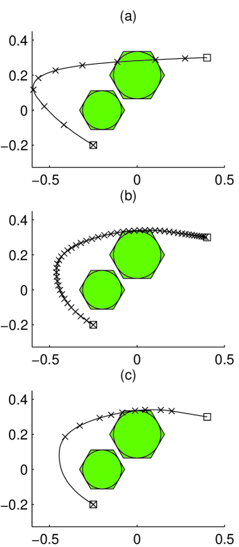
Figure 1: Figure (a) shows the resulting trajectory using uniform gridding ($N_{o}=10$), Figure (b) shows the trajectory using a finer uniform gridding ($N_{o}=50$), and Figure (c) shows the trajectory using iterative MILP avoidance ($N_{o}=9$). The circles denote obstacles, and the polygons denote the buffer regions used in the MILP formulation. The values of the parameters are $M_{o}=6$, $M_{u}=4$, $N_{u}=4$, $(x_{s},y_{s},\dot{x}_{s},\dot{y}_{s})=(-0.25,-0.2,-0.5,0.3)$, and $(x_{f},y_{f},\dot{x}_{f},\dot{y}_{f})=(0.4,0.3,0,0)$.

A simple method to reduce this behavior is to take a finer discretization, which increases the number avoidance times, as shown in Figure 1(b). However, this is not desirable in MILP because an increase in the number of avoidance times increases the number of binary variables in the problem.

3.2 Iterative MILP time step selection algorithm

It is advantageous to use as few avoidance times as possible. Next, we propose an iterative algorithm to do so. The method distributes avoidance times where they are needed most, as shown in Figure 1(c), and guarantees obstacle avoidance if an obstacle free trajectory exists. The idea is to first solve the MILP with no obstacle avoidance times (or with a coarse set of avoidance times) and check the resulting trajectory for collisions. Then, if there are collisions, augment the MILP formulation with an avoidance time (and the corresponding binary variables and constraints) for each collision. The avoidance time for each collision is taken from the interval of time that the trajectory is within the obstacle. Next, solve the augmented MILP and check the resulting trajectory for collisions, repeating the procedure until a collision free trajectory is found.

Table 1: Iterative MILP time step selection algorithm

1:  Formulate vehicle control problem as a MILP with the set of obstacle avoidance times $\{t_{o}[k]\}_{k=1}^{N_{o}}$. 2:  Set obstacle buffer zone for each obstacle $j$, $R_{buff}^{(j)}:=\alpha R_{obst}^{(j)}$ where $\alpha>1$. 3:  Solve MILP with obstacles of radius $R_{buff}^{(j)}$ for each obstacle $j$. 4:  Check resulting trajectory for collisions with obstacles of radius $R_{obst}^{(j)}$ for each obstacle $j$. 5:  while there are collisions do 6:     For each collision $i$, compute time interval $[t_{1}^{(i)},t_{2}^{(i)}]$. 7:     For each collision $i$, augment the MILP formulation with obstacle avoidance constraints at time $t_{o}^{new}\in[t_{1}^{(i)},t_{2}^{(i)}]$. 8:     Solve augmented MILP with obstacles of radius $R_{buff}^{(j)}$ for each obstacle $j$. 9:     Check resulting trajectory for collisions with obstacles of radius $R_{obst}^{(j)}$ for each obstacle $j$. 10:  end while

The algorithm is outlined in Table 1 and proceeds as follows: First, formulate the vehicle control problem as a MILP and choose an initial set of avoidance times $\{t_{o}[k]\}_{k=1}^{N_{o}}$. This set is usually taken to be the empty set or a coarsely distributed set of times. Next, introduce a buffer zone for each obstacle $j$ with radius $R_{buff}^{(j)}=\alpha R_{obst}^{(j)}$, where $\alpha>1$ is the buffer factor. Radius $R_{buff}^{(j)}$ is larger than $R_{obst}^{(j)}$ (usually taken slightly larger) and is used as the radius of obstacle $j$ in the MILP formulation. This is done to guarantee obstacle avoidance and termination of the algorithm, which we show later in this section. Next, solve the MILP using the buffer regions as the obstacles. Then, check the resulting trajectory for collisions using each obstacle’s true radius, $R_{obst}^{(j)}$ for each obstacle $j$. To check for collisions, sample the trajectory and check whether or not each sample point is inside any of the obstacles.

If there are no collisions, terminate the algorithm. Otherwise, for each collision $i$, compute the time interval $[t_{1}^{(i)},t_{2}^{(i)}]$ in which the trajectory is within the obstacle. This interval can be computed efficiently using a bisection routine and the collision check routine. Then, for each collision $i$, augment the MILP problem formulation with avoidance constraints at time $t_{o}^{new}$ taken to be in the interval $[t_{1}^{(i)},t_{2}^{(i)}]$. In this paper, we take $t_{o}^{new}=(t_{1}^{(i)}+t_{2}^{(i)})/2$. Next, solve the augmented MILP and check the resulting trajectory for collisions. If there are no collisions, terminate the algorithm. Otherwise, repeat the procedure until there are no collisions.

Snapshots of intermediate steps in the iterative algorithm are shown in Figure 2. The procedure adds obstacle avoidance points where they are needed most, thus avoiding unnecessary and computationally costly constraints and binary variables.

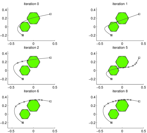
Figure 2: Snapshots of the iterative MILP obstacle avoidance algorithm. The circular regions denote obstacles, and the polygons denote the buffer regions used in the MILP formulation. Each cross ‘$\times$’ denotes a time at which obstacle avoidance is enforced. The values of the parameters are $M_{o}=6$, $M_{u}=4$, $N_{u}=4$, $(x_{s},y_{s},\dot{x}_{s},\dot{y}_{s})=(-0.25,-0.2,-0.5,0.3)$, and $(x_{f},y_{f},\dot{x}_{f},\dot{y}_{f})=(0.4,0.3,0,0)$.

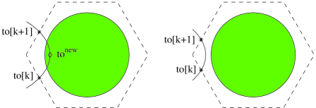
Figure 3: These diagrams help show that the iterative MILP time selection algorithm terminates. If the difference between consecutive obstacle avoidance times, denoted $t_{o}[k+1]-t_{o}[k]$, is greater than $2\Delta t_{\min}$, the trajectory can intersect the obstacle as shown in the figure on the left. In this case, the algorithm will add a new avoidance constraint at time $t_{o}^{new}$. If the difference is less than $2\Delta t_{\min}$, the trajectory can not intersect the obstacle, and a new avoidance constraint can not be added in between.

Now we show that the iterative algorithm in Table 1 terminates. The minimum distance between the boundary of a buffer zone and the boundary of the obstacle it surrounds is $d=R_{buff}-R_{obst}=(\alpha-1)R_{obst}$. For a problem involving multiple obstacles, the minimum of these distances is given by $d_{\min}=(\alpha-1)R_{obst}^{\min}$, where $R_{obst}^{\min}$ is the radius of the smallest obstacle in the environment. The minimum time it takes the vehicle to travel between the boundary of a buffer zone and its corresponding obstacle is given by $\Delta t_{\min}=d_{\min}/v_{\max}=(\alpha-1)R_{obst}^{\min}/v_{\max}$, where $v_{\max}$ is the maximum velocity of the vehicle. Consider two consecutive obstacle avoidance times denoted $t_{o}[k]$ and $t_{o}[k+1]$. The vehicle must be located outside all buffer zones at these two times because we have enforced this as a hard constraint in the MILP. If the difference $t_{o}[k+1]-t_{o}[k]$ is less than $2\Delta t_{\min}$, the vehicle’s trajectory can not intersect the obstacle because there is not enough time to enter the buffer zone, collide with the obstacle, then exit the buffer zone (see Figure 3). In order for the trajectory to intersect the obstacle in the interval between these two times, the difference $t_{o}[k+1]-t_{o}[k]$ must be greater than $2\Delta t_{\min}$. In summary, the algorithm will not add an obstacle avoidance time in the interval if $t_{o}[k+1]-t_{o}[k]<2\Delta t_{\min}$, but it can add an obstacle avoidance time if $t_{o}[k+1]-t_{o}[k]\geq 2\Delta t_{\min}$. Therefore, in the worst case, once the algorithm reaches a point where the time interval between each obstacle avoidance time is less than $2\Delta t_{\min}$, the algorithm must terminate.

Next we bound the number of steps it takes for the algorithm to terminate. The smallest possible time interval between consecutive obstacle avoidance times is $\Delta t_{\min}$. This can be seen by looking at Figure 4, where $t_{o}[k+1]$ and $t_{o}[k]$ are two consecutive avoidance times and $t_{1}$ is the time at which the trajectory enters the obstacle and $t_{2}$ is the time it exits the obstacle. Suppose the vehicle is moving at its maximum velocity from time $t_{o}[k]$ to $t_{1}$. The algorithm will detect this intersection, compute times $t_{1}$ and $t_{2}$, and pick a new obstacle avoidance time $t_{o}^{new}$ in the interval $[t_{1},t_{2}]$. Suppose the algorithm picks $t_{o}^{new}=t_{1}$, then $t_{o}^{new}-t_{o}[k]=\Delta t_{\min}$. The time interval can not be any less because the vehicle can not pass through the buffer zone in time less than $\Delta t_{\min}$. In the trajectory generation problem, if $t_{s}$ is the vehicle’s starting time and $t_{f}$ is its finishing time, the maximum number of time intervals added by the algorithm is $\lfloor(t_{f}-t_{s})/\Delta t_{\min}\rfloor$. Therefore, the algorithm will terminate in a maximum of $\lfloor(t_{f}-t_{s})/\Delta t_{\min}\rfloor$ steps. This is a worst case result. In practice the algorithm terminates in fewer steps.

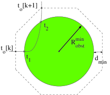
Figure 4: This diagram helps show the minimum time step that can be added by the iterative MILP time step selection algorithm. The trajectory intersects the obstacle in the interval $[t_{1},t_{2}]$. Assume the vehicle is moving at $v_{\max}$ between times $t_{o}[k]$ and $t_{1}$. If the algorithm selects $t_{1}$ as the new obstacle avoidance time, the difference $t_{1}-t_{o}[k]$ is equal to $\Delta t_{\min}$. This is the minimum possible time interval between avoidance times because the vehicle can not move any faster.

3.3 Iterative MILP obstacle growing algorithm

Being consistent with our goal to reduce the number of obstacle avoidance times in our MILP problem formulations, we propose another iterative MILP algorithm for obstacle avoidance. This algorithm iteratively grows the buffer zones surrounding the obstacles until a collision free trajectory is found. The idea is to first solve the MILP with a coarse set of avoidance times and an initial set of buffer zones surrounding each obstacle. Then, check the resulting trajectory for collisions. If there are collisions, increase the size of each buffer zone that surrounds an obstacle with which the trajectory collides. Next, solve the MILP with these new buffer zones and check the resulting trajectory for collisions. This process is repeated until there are no collisions.

The details of the algorithm are listed in Table 2. Snapshots of intermediate steps of the algorithm are shown in Figure 5. The crosses denote the coarse set of times at which obstacle avoidance is enforced in the MILP. As the figure shows, the size of the buffer regions surrounding the obstacles with which the trajectory intersects is increased until the resulting trajectory, generated by the MILP, avoids all obstacles.

The situation in which this algorithm is most useful is when uniform gridding is used and the resulting trajectory clips an obstacle, barely intersecting it. In this case, the algorithm pushes the trajectory away from the clipped obstacle in a few iterations, resulting in a collision free trajectory. However, if the initial distribution of avoidance times is too coarse, the algorithm could have problems. In this case, the buffer regions could grow to be large and engulf the initial or final position, which results in an infeasible MILP.

Table 2: Iterative MILP obstacle growing algorithm

1:  Formulate vehicle control problem as a MILP with the set of obstacle avoidance times $\{t_{o}[k]\}_{k=1}^{N_{o}}$. 2:  Set obstacle buffer zone for each obstacle $j$, $R_{buff}^{(j)}:=\alpha R_{obst}^{(j)}$ where $\alpha>1$. 3:  Solve MILP with obstacles of radius $R_{buff}^{(j)}$ for each obstacle $j$. 4:  Check resulting trajectory for collisions with obstacles of radius $R_{obst}^{(j)}$ for each obstacle $j$. 5:  while there are collisions do 6:     For each obstacle $j$ that collides with the trajectory, increase buffer region by setting $R_{buff}^{(j)}:=\alpha R_{buff}^{(j)}$. 7:     Solve MILP with obstacles of radius $R_{buff}^{(j)}$ for each obstacle $j$. 8:     Check resulting trajectory for collisions with obstacles of radius $R_{obst}^{(j)}$ for each obstacle $j$. 9:  end while

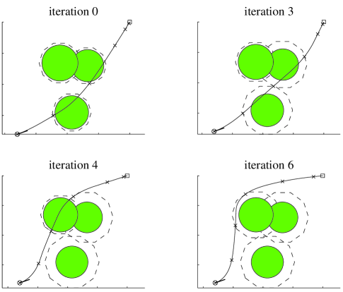
Figure 5: Snapshots of the iterative MILP obstacle growing algorithm. The circular regions denote obstacles, and the polygons denote the buffer regions used in the MILP formulation. Each cross denotes a time at which obstacle avoidance is enforced.

3.4 Average case complexity

In this section, we explore the average case computational complexity of the iterative MILP obstacle avoidance algorithm by solving randomly generated problem instances. Each instance is generated by randomly picking parameters from a uniform distribution over the intervals defined below. Each MILP is solved using AMPL [13] and CPLEX [15] on a PC with Intel PIII 550MHz processor, 1024KB cache, 3.8GB RAM, and Red Hat Linux. For all instances solved, processor speed was the limiting factor, not memory.

For comparison, we solve the same instances using uniform gridding with sample time $\Delta t_{c}=2R_{obst}^{\min}\sqrt{\alpha^{2}-1}/v_{\max}$. This sample time is the maximum sample time that guarantees obstacle avoidance, assuming the vehicle travels in a straight line between sample times. This is a good approximation since $\Delta t_{c}$ is small for the instances we solve. See Appendix A for details. Each obstacle avoidance time is given by $t_{o}[k]=k\Delta t_{c}$, where $k=1,\ldots,N_{o}$ and $N_{o}=\lceil t_{f}/\Delta t_{c}\rceil$.

The instances are generated as follows: The start state is taken to be $\mathbf{x}_{s}=(x_{s},y_{s},r_{v}\cos\theta_{v},r_{v}\sin\theta_{v})$, where $(x_{s},y_{s})$ is constant, and $r_{v}$ and $\theta_{v}$ are random variables chosen uniformly from the intervals $[r_{v}^{\min},r_{v}^{\max}]$ and $(0,2\pi]$, respectively. The final state is fixed with zero velocity, $\mathbf{x}_{f}=(x_{f},y_{f},0,0)$. We generate $N_{obst}$ obstacles each with position $(x_{obst},y_{obst})=(r\cos\theta,r\sin\theta)$ and radius $R_{obst}$. The parameters $R_{obst}$, $r$, and $\theta$ are random variables chosen uniformly from the respective intervals $[R_{\min},R_{\max}]$, $[r_{\min},r_{\max}]$, and $(0,2\pi]$ such that no obstacle overlaps the circle of radius $R_{s}$ with position $(x_{s},y_{s})$ or the circle of radius $R_{f}$ with position $(x_{f},y_{f})$.

For the instances generated in this paper, we set the intervals to be $r_{v}\in[0.5,1.0]$, $R_{obst}\in[0.2,0.3]$, and $r\in[0.0,1.0]$. The constant parameters are taken to be $(x_{s},y_{s})=(-0.8,-0.8)$, $(x_{f},y_{f})=(1.0,1.0)$, $R_{s}=0.5$, and $R_{f}=0.1$.

The solution to an instance of the obstacle avoidance problem with three obstacles is shown in Figure 6 for the the uniform gridding method and for the iterative MILP methods. Each cross denotes the time along the trajectory at which obstacle avoidance is enforced. The uniform gridding method with sample time $\Delta t_{c}$ requires $N_{o}=25$ obstacle avoidance times, shown in Figure 6(b), while the iterative MILP time step selection algorithm requires only $N_{o}=4$ avoidance times, shown in Figure 6(c). Notice the efficiency in which the iterative algorithm distributes the avoidance times. For comparison, we also solve this instance using uniform gridding with sample time $2\Delta t_{\min}$ (Figure 6(a)) and using the iterative obstacle growing algorithm (Figure 6(d)). For uniform gridding, choosing sample time $2\Delta t_{\min}$ guarantees obstacle avoidance as discussed in Section 3.2. However, as shown in the figure, this dense set of obstacle avoidance times is very conservative.

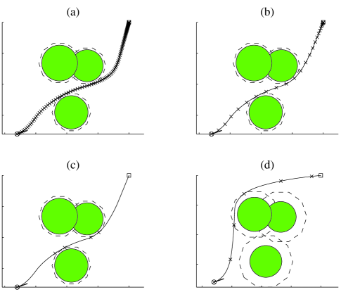
Figure 6: Solutions to an instance of the obstacle avoidance problem using: (a) uniform gridding with sample time $2\Delta t_{\min}$ ($N_{o}=115$), (b) uniform gridding with sample time $\Delta t_{c}$ ($N_{o}=25$), (c) iterative time step selection ($N_{o}=4$), and (d) iterative obstacle growing ($N_{o}=5$). The straight line segment denotes the initial velocity $(\dot{x}_{s},\dot{y}_{s})=(0.497,0.172)$, the circular regions denote obstacles, the dashed regions denote the polygonal buffer zones, and each cross denotes a time along the trajectory at which obstacle avoidance is enforced.

In Figure 7, we plot the fraction of instances solved versus computation time for the two methods. As these figures show, the iterative MILP method is less computationally intensive than the uniform gridding method for the instances solved. For example, 70% of the instances are solved in 0.4 seconds or less using the iterative MILP algorithm for the 3 obstacle case. In contrast, no instances are solved in 0.4 seconds or less using uniform gridding for the 3 obstacle case.

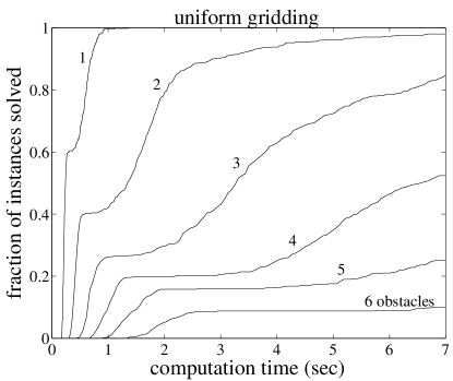
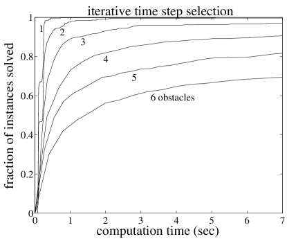
Figure 7: Fraction of instances solved versus computation time for uniform gridding (top) and the iterative MILP obstacle avoidance (bottom). We consider $N_{obst}=2,3,4$. For each curve, 500 random instances were solved. The values of the parameters are $N_{u}=10$, $M_{u}=10$, and $M_{o}=10$.

In Figure 8, we plot the computation time necessary to solve 70% of the randomly generated instances versus the number of obstacles on the field. Data is plotted for the uniform gridding method and for the iterative MILP method. The computational requirements for both methods grow exponentially with the number of obstacles. However, as the figure shows, the iterative MILP method is less computationally intensive and the computation time grows at a slower rate.

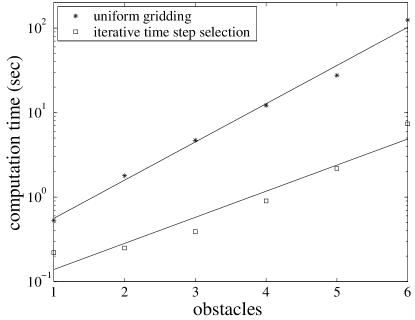
Figure 8: Computation time necessary to solve 70% of the randomly generated instances versus the number of obstacles. Each square denotes a data point for the uniform gridding method. Each asterisk denotes a data point for the iterative MILP method. The solid lines denote curves fitted to these data.

4 Minimum time problems

In this section, we present an iterative MILP algorithm for solving minimum time problems using a vehicle trajectory generation problem as motivation. In [21, 22], MILP methods for this problem are presented. Time is discretized uniformly and the sampling interval that contains the optimal time is found using MILP. To get better bounds on the optimal time, the sample time of the discretization must be reduced, which results in a larger number of binary variables. In Appendix B, this method is outlined in the context of the vehicle considered in this paper.

Here we propose an iterative algorithm that converges to the optimal time using binary search. At each iteration the feasibility of a MILP is determined using a solver such as CPLEX [15]. In each MILP, the number of binary variables and the number of constraints are much fewer than those for other techniques because only one discrete time step is needed.

To motivate the iterative algorithm we consider a minimum time vehicle control problem. Given a vehicle governed by equations (9) and (11), find the sequence of control inputs $\{\mathbf{u}[k]\}_{k=0}^{N_{u}-1}$ that transfers the vehicle from initial state $\mathbf{x}(0)=\mathbf{x}_{s}$ to final state $\mathbf{x}(t_{f})=\mathbf{x}_{f}$ in minimum time.

Suppose we know that the optimal time, denoted $t^{*}$, is within the time interval $(t_{L},t_{R}]$. Let time $t_{M}=(t_{L}+t_{R})/2$. Consider the MILP given by equation (9), equation (11), constraint $\mathbf{x}(0)=\mathbf{x}_{s}$, and constraint $\mathbf{x}(t_{f})=\mathbf{x}_{f}$ with final time taken to be $t_{f}=t_{M}$. We use equation (10) to express $\mathbf{x}(t_{f})$ in terms of the control inputs. To determine if there exists a sequence of control inputs that transfers the vehicle from start state to finish state, we solve the MILP without an objective function (this is a feasibility problem).

If the MILP is feasible, $t^{*}$ must be within the interval $(t_{L},t_{M}]$. Otherwise, the MILP is infeasible and $t^{*}$ must be within the interval $(t_{M},t_{R}]$. By determining the feasibility of the MILP, we have cut the bound on the optimal time $t^{*}$ in half. This suggests an iterative binary search procedure that converges to $t^{*}$.

The iterative algorithm is outlined in Table 3 and proceeds as follows: First, pick a time interval $(t_{lb},t_{ub}]$ that bounds the optimal time $t^{*}$. The lower bound is taken to be $t_{lb}=d_{\min}/v_{\max}$, where $d_{\min}$ is the straight line distance from the initial position to the final position and $v_{\max}$ is the maximum velocity of the vehicle. The upper bound is taken to be a feasible time in which the vehicle can reach the destination. A simple way to compute a feasible time is to try time $\alpha t_{lb}$, where $\alpha>1$, increasing $\alpha$ until a feasible time is found. Set $t_{L}:=t_{lb}$, $t_{R}:=t_{ub}$, and $t_{M}:=(t_{R}+t_{L})/2$.

Next, set the final time in the MILP problem formulation to be $t_{f}=t_{M}$, and determine if the resulting MILP is feasible using the MILP solver. If the MILP is feasible, the optimal time $t^{*}$ must be within the interval $(t_{L},t_{M}]$. In this case, set $t_{R}:=t_{M}$. Otherwise, the MILP is infeasible and the vehicle can not reach the destination in time $t_{M}$. The optimal time $t^{*}$ must be within the interval $(t_{M},t_{R}]$. In this case, set $t_{L}:=t_{M}$. Then, update $t_{M}$ by setting $t_{M}:=(t_{R}+t_{L})/2$. If the difference $t_{R}-t_{L}$ is less than some desired tolerance for our calculation of $t^{*}$, denoted $\epsilon$, the algorithm terminates. Otherwise, repeat the process by setting the final time to $t_{f}=t_{M}$ and continue with the steps outlined previously until the computed value of $t^{*}$ is within the desired tolerance $\epsilon$.

After the $k$th iteration, the time interval containing optimal time $t^{*}$ has length $(t_{ub}-t_{lb})/2^{k}$.

Table 3: Iterative minimum time MILP algorithm

1:  Formulate problem as a MILP without objective function. 2:  Set $t_{L}:=t_{lb}$ and $t_{R}:=t_{ub}$. 3:  Set $t_{M}:=(t_{R}+t_{L})/2$. 4:  while $(t_{R}-t_{L})>\epsilon$ do 5:     Determine feasibility of MILP with final time $t_{f}=t_{M}$. 6:     if feasible then set $t_{R}:=t_{M}$. 7:     else set $t_{L}:=t_{M}$. 8:     Set $t_{M}:=(t_{R}+t_{L})/2$. 9:  end while

The solid lines of Figure 9 show the solution to an instance of the minimum time problem. The iterative procedure was stopped after thirteen iterations, which took approximately one second on our Pentium III 550 MHz computer. To achieve the same accuracy using the uniform time discretization method, solving one large MILP with a small sampling time, it took five minutes on the same computer.

Our iterative procedure converges to the time optimal solution of the problem stated in the beginning of this section. This solution is an approximate solution to the continuous time version of the minimum time vehicle control problem. In the continuous time version of the problem, the vehicle is governed by equations (8) and (7). We wish to transfer the vehicle from starting state $\mathbf{x}_{s}$ to finishing state $\mathbf{x}_{f}$ in minimum time. In Figure 9, we compare our near optimal solution to the continuous time problem (solid lines) to another technique (dotted lines) for generating near optimal solutions from [18], which was used successfully in the RoboCup competition.

In addition to being used on its own, our iterative approach can be combined with the uniform discretization approach. In this case, the uniform approach is run first with a coarse discretization (large sampling time $T$). The output is a time interval of size $T$, which contains the optimal time $t^{*}$. We use this time interval as the input to our iterative algorithm. The $k$th step of the iterative algorithm outputs a time interval of length $T/2^{k}$ containing the optimal time $t^{*}$, and thus quickly converges to the optimal time.

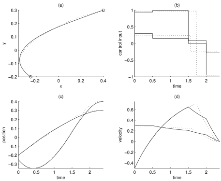
Figure 9: Time optimal solution (solid lines) to an instance of the minimum time vehicle control problem of Section 4 given by the iterative MILP algorithm. For comparison we plot the near optimal solution (dotted lines) for the continuous time version of the problem obtained using techniques from [18]. The parameters are: $M_{u}=20$, $N_{u}=10$, $(x_{s},y_{s},\dot{x}_{s},\dot{y}_{s})=(-0.25,-0.2,-0.5,0.3)$, $(x_{f},y_{f},\dot{x}_{f},\dot{y}_{f})=(0.4,0.3,0,0)$.

5 Discussion

We have presented iterative MILP algorithms for obstacle avoidance and for minimum time control problems. The iterative MILP time selection algorithm picks obstacle avoidance times and intelligently distributes them where they are needed most. The iterative MILP obstacle growing algorithm allows a course set of obstacle avoidance times to be used instead of a dense distribution, which is required to guarantee obstacle avoidance for standard MILP methods. Both of these algorithms reduce the number of binary variables needed to formulate and solve obstacle avoidance trajectory generation problems using MILP. To demonstrate the computational benefits of the iterative MILP time step selection algorithm, we performed an average case computational complexity analysis. For comparison, we also performed the analysis on the standard uniform gridding method. The iterative algorithm significantly outperformed the uniform gridding method. In addition, we also present an iterative algorithm for solving minimum time problems using MILP. We found that the algorithm significantly outperforms standard techniques for minimum time problems using MILP.

Due to the reduced computational requirements of these methods, they can be applied more widely in practice. Computational efficiency is especially important for real time control in dynamically changing environments where new control plans need to be generated often and in real time using a strategy such as model predictive control [16]. In our research [8, 9], we use these methods to solve cooperative control problems such as those described in [4, 6, 7]. However, there is much room for improvement, including decreasing computation time further and developing methods that scale better with increased numbers of obstacles and vehicles. In [8] we discuss ideas to further decrease the computational requirements of MILP methods. We feel that intelligent time step selection methods, such as those presented in this paper, can be very useful in reducing computational requirements and should be pursued further. One aspect that needs inspection is the intelligent selection of the discretization for the control input to the vehicle.

Appendix A Appendix: Sample time

Here we derive the minimum sample time, denoted $\Delta t_{c}$, that guarantees obstacle avoidance between sample times, assuming the vehicle moves in a straight line path between sample times. This is a good approximation, because $\Delta t_{c}$ is small for the problems we solve.

Let $d$ be the straight line distance the vehicle can travel between any two consecutive avoidance times. The cord of the smallest buffer region that is tangent to the obstacle it surrounds is denoted the critical cord. The critical cord length is given by $d_{c}=2((R_{buff}^{\min})^{2}-(R_{obst}^{\min})^{2})^{1/2}=2R_{obst}^{\min}\sqrt{\alpha^{2}-1}$ because $R_{buff}^{\min}=\alpha R_{obst}^{\min}$.

If $d<d_{c}$, the vehicle is guaranteed to avoid the obstacle between avoidance times. If $d\geq d_{c}$, the vehicle can collide with the obstacle between avoidance times. The critical time interval $\Delta t_{c}$ is given by

$$\Delta t_{c}=\frac{d_{c}}{v_{\max}}=\frac{2R_{obst}^{\min}\sqrt{\alpha^{2}-1}}{v_{\max}},$$ (18)

where $v_{\max}$ is the maximum velocity of the vehicle.

Appendix B Appendix: Minimum time MILP formulation

Here we consider a minimum time trajectory generation problem. We are given a vehicle governed by the discrete time system (9) and subject to the constraints (11). The objective is to find the sequence of control inputs $\{\mathbf{u}[k]\}_{k=0}^{N_{u}-1}$ that transfers the system from the initial state $\mathbf{x}(0)=\mathbf{x}_{s}$ to the final state $\mathbf{x}(t_{f})=\mathbf{x}_{f}$ in minimum time.

Applying the techniques of [21, 22], we introduce a uniform time discretization with constant sampling time $T$. The solution of the resulting MILP gives a feasible time that is within $T$ of the optimal time.

Discretize time into $N_{T}$ times given by $t_{T}[k]=kT$, where $k$ is an element of the set $\{1,\ldots,N_{T}\}$. The discretization must be chosen so that $t_{T}[N_{T}]=N_{T}T$ is larger than the optimal time.

Next, introduce auxiliary binary variable $\delta[k]\in\{0,1\}$ and the inequality constraints,

$$x(t_{T}[k])-x_{f}\leq H(1-\delta[k])$$

$$x(t_{T}[k])-x_{f}\geq-H(1-\delta[k])$$

$$y(t_{T}[k])-y_{f}\leq H(1-\delta[k])$$

$$y(t_{T}[k])-y_{f}\geq-H(1-\delta[k])$$

$$\dot{x}(t_{T}[k])-\dot{x}_{f}\leq H(1-\delta[k])$$

$$\dot{x}(t_{T}[k])-\dot{x}_{f}\geq-H(1-\delta[k])$$

$$\dot{y}(t_{T}[k])-\dot{y}_{f}\leq H(1-\delta[k])$$

$$\dot{y}(t_{T}[k])-\dot{y}_{f}\geq-H(1-\delta[k]),$$ (19)

for each $k$ in the set $\{1,\ldots,N_{T}\}$. Here, the state $\mathbf{x}(t_{T}[k])$ is written in terms of the control inputs using equation (10), and $H$ is a large positive constant taken to be greater than the largest dimension of the operating environment.

If $\delta[k]=0$, every constraint in equation (19) is trivially satisfied because, for example, $x(t_{T}[k])-x_{f}$ is always less than $H$. Otherwise, $\delta[k]=1$ and the constraints in equation (19) enforce the condition $\mathbf{x}(t_{T}[k]=\mathbf{x}_{f})$. To require that the final condition be satisfied at only one discrete time $t_{T}[k]$ the following constraint is introduced,

$$\sum_{i=1}^{N_{T}}\delta[i]=1.$$ (20)

Finally, we introduce the cost function to be minimized,

$$J=\sum_{i=1}^{N_{T}}i\delta[i].$$ (21)

By minimizing this cost the final state $\mathbf{x}_{f}$ is reached at the earliest discrete time, $t_{T}[k]$, possible. The output after solving the resulting MILP is a single $k_{sol}$ such that $\delta[k_{sol}]=1$. The optimal time is therefore within the interval $(t_{T}[k_{sol}-1],t_{T}[k_{sol}]]$.

References

- [1] J. S. Bellingham, M. Tillerson, M. Alighanbari, and J. P. How, “Cooperative Path Planning for Multiple UAVs in Dynamic and Uncertain Environments,” Proc. IEEE Conf. Decision and Control, Las Vegas, Neveda, Dec. 2002, pp. 2816–2822.
- [2] A. Bemporad and M. Morari, “Control of Systems Integrating Logic, Dynamics, and Constraints,” Automatica, vol. 35, pp. 407–428, 1999.
- [3] D. Bertsimas and J. N. Tsitsiklis, Introduction to Linear Optimization, Athena Scientific, Belmont, Massachusetts, 1997.
- [4] M. Campbell, R. D’Andrea, D. Schneider, A. Chaudhry, S. Waydo, J. Sullivan, J. Veverka, and A. Klochko, “RoboFlag Games Using Systems Based, Hierarchical Control,” Proceedings of the American Control Conference, June 4–6, 2003, pp. 661–666.
- [5] R. D’Andrea, T. Kalmár-Nagy, P. Ganguly, and M. Babish, “The Cornell RoboCup Team,” In G. Kraetzschmar, P. Stone, T. Balch Eds., Robot Soccer WorldCup IV, Lecture Notes in Artificial Intelligence, Springer, 2001.
- [6] R. D’Andrea and R. M. Murray, “The RoboFlag Competition,” Proceedings of the American Control Conference, June 4–6, 2003, pp. 650–655.
- [7] R. D’Andrea and M. Babish, “The RoboFlag Testbed,” Proceedings of the American Control Conference, June 4–6, 2003, pp. 656–660.
- [8] M. G. Earl and R. D’Andrea, “Multi-vehicle Cooperative Control Using Mixed Integer Linear Programming,” A preprint is available at cs/0501092
- [9] M. G. Earl and R. D’Andrea, “A Decomposition Approach to Multi-vehicle Cooperative Control,” A preprint is available at cs/0504081
- [10] M. G. Earl and R. D’Andrea, “A Study in Cooperative Control: The RoboFlag Drill,” Proceedings of the American Control Conference, Anchorage, Alaska May 8–10, 2002, pp. 1811–1812.
- [11] M. G. Earl and R. D’Andrea, “Modeling and Control of a Multi-agent System Using Mixed Integer Linear Programming,” Proc. IEEE Conf. Decision and Control, Las Vegas, Nevada, Dec. 2002, pp. 107–111.
- [12] All files for generating the plots found in this paper are available online at http://control.mae.cornell.edu/earl/milp2
- [13] R. Fourer, D. M. Gay, B. W. Kernighan, “AMPL–A Modeling Language For Mathematical Programming,” Boyd & Fraser, 1993. http://www.ampl.com
- [14] M. R. Garey and D. S. Johnson. Computers And Intractability: A guide to the Theory of NP-Completeness. W. H. Freeman and Co., 1979.
- [15] ILOG AMPL CPLEX System Version 7.0 User’s Guide, 2000. http://www.ilog.com/products/cplex
- [16] D. Q. Mayne, J. B. Rawlings, C. V. Rao, and P. O. M. Scokaert, “Constrained Model Predictive Control: Stability and Optimality,” Automatica, vol. 36, pp. 789–814, 2000.
- [17] M. Morari, M. Baotic, and F. Borrelli, “Hybrid Systems Modeling and Control,” European Journal of Control, Vol. 9, No. 2-3, pp. 177-189, 2003.
- [18] T. Kalmár-Nagy, R. D’Andrea, and P. Ganguly. “Near-Optimal Dynamic Trajectory Generation and Control of an Omnidirectional Vehicle,” Robotics and Autonomous Systems, vol. 46, pp. 47–64, 2004.
- [19] J. Ousingsawat and M. E. Campbell, “Establishing Optimal Trajectories for Multi-vehicle Reconnaissance,” AIAA Guidance, Navigation and Control Conference, 2004.
- [20] A. Richards, T. Schouwenaars, J. P. How, and E. Feron, “Spacecraft Trajectory Planning with Avoidance Constraints Using Mixed-Integer Linear Programming,” Journal of Guidance, Control, and Dynamics, Vol. 25, pp. 755–764, July–August 2002.
- [21] A. Richards and J. P. How, “Aircraft Trajectory Planning With Collision Avoidance Using Mixed Integer Linear Programming,” Proc. American Control Conf., Anchorage, Alaska May 8–10, 2002.
- [22] H. P. Rothwangl, “Numerical Synthesis of the Time Optimal Nonlinear State Controller via Mixed Integer Programming,” Proc. American Control Conf., Arlington, VA, June 2001, pp. 3201–3205.
- [23] P. Stone, M. Asada, T. Balch, R. D’Andrea, M. Fujita, B. Hengst, G. Kraetzschmar, P. Lima, N. Lau, H. Lund, D. Polani, P. Scerri, S. Tadokoro, T. Weigel, and G. Wyeth, “RoboCup-2000: The Fourth Robotic Soccer World Championships,” AI MAGAZINE, vol. 22(1), pp. 11–38, Spring 2001.