Broadcast Channels with Cooperating Decoders

Abstract

We consider the problem of communicating over the general discrete memoryless broadcast channel (BC) with partially cooperating receivers. In our setup, receivers are able to exchange messages over noiseless conference links of finite capacities, prior to decoding the messages sent from the transmitter. In this paper we formulate the general problem of broadcast with cooperation. We first find the capacity region for the case where the BC is physically degraded. Then, we give achievability results for the general broadcast channel, for both the two independent messages case and the single common message case.

I introduction

I-A Motivation

In the classic broadcast scenario the receivers decode their messages independently of each other. However, the increasing interest in networking motivates the consideration of broadcast scenarios in which each node in the network, besides decoding its own information, tries to help other nodes in decoding. This problem comes up naturally in sensor networks, where a transmitter external to the sensor network wants to download data into the network, e.g., to configure the sensor array. The concept of cooperation among receivers is also relevant to general ad-hoc networks, since such cooperation provides a method for increasing the rates without increasing the spectrum allocation. Therefore, this motivates the study of the effect of receiver cooperation on the rates for the broadcast channel.

I-B The Discrete Memoryless Broadcast Channel (DMBC)

The broadcast channel was introduced by Cover in [1]. Following this initial work, Bergmans proved an achievability result for the degraded BC, [2], and also a partial converse that holds only for the Gaussian broadcast channel [3]; in [4] Gallager established a converse that holds for any discrete memoryless degraded broadcast channel. In [5] El-Gamal generalized the capacity result for the degraded broadcast channel to the “more capable” case, and in [6] and [7] he showed that feedback does not increase the capacity region for the physically degraded case. Several other classes of broadcast channels were studied in the following years. For example, the sum and product of two degraded broadcast channels were considered in [8], and in [9], [10] and [11] the deterministic broadcast channel was analyzed.

For the general broadcast channel, Cover derived an achievable rate region for the case of two independent senders in [12]. In [13] Korner and Marton considered the capacity of general broadcast channels with degraded message sets. The best achievable region and the best upper bound for the two independent senders case were derived by Marton in [14], and a simple proof of Marton’s achievable region appeared later in [15]. Another upper bound for the general broadcast channel, the so-called degraded, same-marginals (DSM) bound, was presented in [16]. This bound is weaker than the upper bound in [14] but stronger than Sato’s upper bound previously presented in [17]. We note, however, that while Marton’s upper bound is the strongest, it is valid only for the two-receiver case, while Sato’s bound and the DSM bound can be extended to more than two receivers. The effect of feedback on the capacity of the Gaussian broadcast channel was studied in [18] and [19], and in [20] the case of correlated sources was considered. A survey on the topic, with extensive references to previous work, can be found in [21]. In recent years the Multiple-Input-Multiple-Output (MIMO) Gaussian broadcast channel has attracted a lot of attention. Initially, the sum-rate capacity was characterized in [22], [23], [24], [25], and finally, in [26] the capacity region was obtained.

None of the early work on the DMBC considered direct cooperation between the receivers.

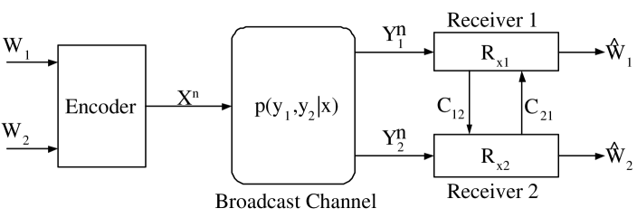
Figure 1: Broadcast channel with two private messages and cooperating receivers.

In the cooperative broadcast scenario, a single transmitter sends two messages to two receivers encoded in a single channel codeword $X^{n}$, where the superscript $n$ denotes the length of a vector. Each of the receivers gets a noisy version of the codeword, $Y_{1}^{n}$ at $R_{x1}$ and $Y_{2}^{n}$ at $R_{x2}$. After reception, the receivers exchange messages over noiseless conference links of finite capacities $C_{12}$ and $C_{21}$, as depicted in Figure 1. The conference messages are, in general, functions of $Y_{1}^{n}$ (at $R_{x1}$), $Y_{2}^{n}$ (at $R_{x2}$), and the previous messages received from the other decoder. After conferencing, each receiver decodes its own message.

We note that in a recent work, [27], the authors consider the problem of interactive decoding of a single broadcast message over the independent broadcast channel by a group of cooperating users. In our work we extend this scenario to the general channel and also consider the two independent senders case.

I-C Cooperative Broadcast: A Combination of Broadcasting and Relaying

The scenario in which one transceiver helps a second transceiver in decoding a message is clearly a relay scenario. Hence, cooperative broadcast can be viewed as a generalization of the broadcast and relay scenarios into a hybrid broadcast/relay system, which better describes future communication networks.

Scenarios of this type have attracted considerable attention recently both from the practical and the theoretical aspects. From the practical aspect, new protocols are proposed for the collaborative broadcast scenario. For example in [28] the authors present a protocol for collaborative decision making involving broadcasting and relaying. From the theoretical aspect, there is a considerable effort invested in characterizing the capacity of an entire network. This work started with [29] and recent results appear in [30] and the following work [31], [32] and [33]. This work focuses on the Gaussian case. A complementing approach for studying the performance of a network is to combine the basic building blocks of a network, namely multiple access, relaying and broadcasting and study the capacity of these combinations. The recent work on relaying focuses on extending the single relay results derived in [34] to the MIMO case (see for example [35]) and to the multiple level case [36], [37]. Another recent result was introduced in [38] where joint decoding was applied to the combined decode-and-forward and estimate-and-forward scheme of [34, theorem 7]. A third approach for studying the performance of an entire network is the network coding approach sparked by the work of [39], which focuses on encoding at the nodes for maximizing the network throughput, separately from the channel coding.

In this paper we focus on the combination of broadcast and relay. A relevant work in this context is [40], in which the capacity of a class of independent relay channels with noiseless relay is derived. Note that the case of noiseless relay is also related to the Wyner-Ziv problem [41]. This relationship will be highlighted in the sequel. Lastly, we note that a recent work, [42], presented an achievability result for the general DMBC with a single wireless cooperation channel from one receiver to the second receiver. This achievable rate region is shown to be the capacity region for the physically degraded broadcast/relay channel.

I-D Main Contributions and Organization

In the following we summarize the main contributions of this work.

• We initially study a special case of the general setup formulated in Section I-B: the case of the physically degraded broadcast channel. Although the physically degraded BC is of little practical interest, it is useful in developing the coding concept for the general BC with cooperation. For the physically degraded BC, we present both an achievability result and a converse. Together, these two results give the capacity region for this setup. Furthermore, this new region is shown to be a strict enlargement of the classical region without cooperation [21].

• Next, we give an achievability result for the general BC with cooperating receivers. This region is also greater, in general, than the classic achievable region given in [14] for the broadcast channel.

• We also consider the case where a single common message is transmitted to both receivers. We consider two different cooperation strategies and derive the achievable rates for each of them. We also derive an upper bound on the achievable rates for this scenario. Here we provide results that explicitly link the available cooperation capacity to the increase in the rate of information. Lastly, we show that for a special case of the general BC, namely when one channel is distinctly better than the other, the upper and lower bounds coincide, resulting in the capacity for that case.

The rest of this paper is structured as follows: in section II we define the mathematical framework. In section III we analyze the physically degraded BC, and derive the capacity region for that case, and in section IV we present an achievability result for the general broadcast channel with cooperating receivers. Next, section V presents achievability results and an upper bound on the rates for the case where only a single common message is transmitted. Concluding remarks are provided in section VI.

II Definitions and Notations

First, a word about notation: in the following we use $H(\cdot)$ to denote the entropy of a discrete random variable (RV), and $I(\cdot;\cdot)$ to denote the mutual information between two discrete random variables, as defined in [43, Ch. 2]. We denote random variables with capital letters – $X$, $Y$, etc., and vectors with boldface letters, e.g., ${\bf x}$, ${\bf y}$. We denote by $A_{\epsilon}^{(n)}(X)$ the weakly typical set for the (possibly vector) random variable $X$, see [43, Ch. 3] for the definition of $A_{\epsilon}^{(n)}(X)$. When referring to a typical set we may omit the random variables from the notation, when these variables are clear from the context. We denote the cardinality of the finite set $\mathcal{A}$ with $||\mathcal{A}||$. We use $\mathcal{X}$ to denote the (discrete and finite) range of $X$. Finally, we denote the probability distribution of the RV $X$ over $\mathcal{X}$ with $p(x)$ and the conditional distribution of $X$ given $Y$ with $p(x|y)$.

Definition 1

A discrete broadcast channel is a channel with discrete input alphabet $\mathcal{X}$, two discrete output alphabets, $\mathcal{Y}_{1}$ and $\mathcal{Y}_{2}$, and a probability transition function, $p(y_{1},y_{2}|x)$. We denote this channel by the triplet $\left(\mathcal{X},p(y_{1},y_{2}|x),\mathcal{Y}_{1}\times\mathcal{Y}_{2}\right)$.

Definition 2

A memoryless broadcast channel is a broadcast channel for which the probability transition function of a sequence of $n$ symbols is given by $p(y_{1}^{n},y_{2}^{n}|x^{n})=\prod_{i=1}^{n}p(y_{1,i},y_{2,i}|x_{i})$, where $y_{k}^{n}=(y_{k,1},y_{k,2},...,y_{k,n})$, $k\in\left\{1,2\right\}$, and $x^{n}=(x_{1},x_{2},...,x_{n})$.

We shall assume the channel to be discrete and memoryless.

Definition 3

The physically degraded broadcast channel is a broadcast channel in which the probability transition function can be decomposed as $p(y_{1},y_{2}|x)=p(y_{1}|x)p(y_{2}|y_{1})$. Hence, for the physically degraded BC we have that $X-Y_{1}-Y_{2}$ form a Markov chain.

Definition 4

An $(R_{12},R_{21})$-conference between $R_{x1}$ and $R_{x2}$ is defined by two conference message sets $\mathcal{W}_{12}=\left\{1,2,...,2^{nR_{12}}\right\}$, $\mathcal{W}_{21}=\left\{1,2,...,2^{nR_{21}}\right\}$, and two mapping functions, $h_{12}$ and $h_{21}$ which map the received sequence of $n$ symbols and the conference messages at one receiver into a message transmitted to the other receiver:

$$h_{12}: \mathcal{Y}_{1}^{n}\times\mathcal{W}_{21}\mapsto\mathcal{W}_{12},$$

$$h_{21}: \mathcal{Y}_{2}^{n}\times\mathcal{W}_{12}\mapsto\mathcal{W}_{21}.$$

We note that this is not the most general definition of a conference, see for example [44], [45] for a more general form. In this paper we consider only conferences in which each receiver sends at most one message to the other receiver. Note that there are cases where a single conference message is enough to achieve capacity: for example, in section III a single conference step achieves capacity for the physically degraded broadcast channel, and in [45] a single conference step achieves capacity for the discrete memoryless multiple access channel counterpart of the setup discussed here.

Definition 5

A $\left(C_{12},C_{21}\right)$-admissible conference is a conference for which $R_{12}\leq C_{12}$ and $R_{21}\leq C_{21}$.

Definition 6

A $\left(\left(2^{nR_{1}},2^{nR_{2}}\right),n,\left(C_{12},C_{21}\right)\right)$ code for the broadcast channel with cooperating receivers having conference links of capacities $C_{12}$ and $C_{21}$ between them, consists of two sets of integers $\mathcal{W}_{1}=\left\{1,2,...,2^{nR_{1}}\right\}$, $\mathcal{W}_{2}=\left\{1,2,...,2^{nR_{2}}\right\}$, called message sets, an encoding function

$$f:\mathcal{W}_{1}\times\mathcal{W}_{2}\mapsto\mathcal{X}^{n},$$

a $\left(C_{12},C_{21}\right)$-admissible conference

$$h_{12}: \mathcal{Y}_{1}^{n}\times\mathcal{W}_{21}\mapsto\mathcal{W}_{12},$$

$$h_{21}: \mathcal{Y}_{2}^{n}\times\mathcal{W}_{12}\mapsto\mathcal{W}_{21},$$

and two decoding functions

$$g_{1}: \mathcal{W}_{21}\times\mathcal{Y}_{1}^{n}\mapsto\mathcal{W}_{1},$$ (1)

$$g_{2}: \mathcal{W}_{12}\times\mathcal{Y}_{2}^{n}\mapsto\mathcal{W}_{2}.$$ (2)

Definition 7

The average probability of error is defined as the probability that the decoded message pair is different from the transmitted message pair:

$$P_{e}^{(n)}=\mbox{Pr}\left(g_{1}(W_{21},Y_{1}^{n})\neq W_{1}\;\;\mbox{or}\;\;g_{2}(W_{12},Y_{2}^{n})\neq W_{2}\right).$$

We also define the average probability of error for each receiver as:

$$P_{e1}^{(n)} = \mbox{Pr}\left(g_{1}\left(W_{21},Y_{1}^{n}\right)\neq W_{1}\right),$$ (3)

$$P_{e2}^{(n)} = \mbox{Pr}\left(g_{2}\left(W_{12},Y_{2}^{n}\right)\neq W_{2}\right),$$ (4)

where we assume transmission of $n$ symbols for each codeword. By the union bound we have that $\max\left\{P_{e1}^{(n)},P_{e2}^{(n)}\right\}\leq P_{e}^{(n)}\leq P_{e1}^{(n)}+P_{e2}^{(n)}$. Hence, $P_{e}^{(n)}\rightarrow 0$ implies that both $P_{e1}^{(n)}\rightarrow 0$ and $P_{e2}^{(n)}\rightarrow 0$, and when both individual error probabilities go to zero then $P_{e}^{(n)}$ goes to zero as well.

In the analysis that follows, we assume that user 1 and user 2 select their respective messages $W_{1}$ and $W_{2}$ independently and uniformly over their respective message sets.

Definition 8

A rate pair $\left(R_{1},R_{2}\right)$ is said to be achievable, if there exists a sequence of $\left(\left(2^{nR_{1}},2^{nR_{2}}\right),n,\left(C_{12},C_{21}\right)\right)$ codes with $P_{e}^{(n)}\rightarrow 0$ as $n\rightarrow\infty$. Obviously, this is satisfied if both $P_{e1}^{(n)}\rightarrow 0$ and $P_{e2}^{(n)}\rightarrow 0$ as $n$ increases.

Definition 9

The capacity region for the discrete memoryless broadcast channel with cooperating receivers is the convex hull of all achievable rates.

III Capacity Region for the Physically Degraded Broadcast Channel with Cooperating Receivers

We consider the physically degraded broadcast channel with three independent messages: a private message to each receiver and a common message to both. We note that for the physically degraded channel, following the argument in [43, theorem 14.6.4], we can incorporate a common rate to both receivers by replacing $R_{2}$, the private rate to the bad receiver, obtained for the two private messages case with $R_{0}+R_{2}$, where $R_{0}$ denotes the rate of the common information. Without cooperation, the capacity region for the physically degraded BC $X-Y_{1}-Y_{2}$ given in [43, theorem 14.6.4], is the convex hull of all the rate triplets $(R_{0},R_{1},R_{2})$ that satisfy

$$R_{1} \leq I(X;Y_{1}|U),$$ (5)

$$R_{0}+R_{2} \leq I(U;Y_{2}),$$ (6)

for some joint distribution $p(u)p(x|u)p(y_{1}|x)p(y_{2}|y_{1})$, where

$$||\mathcal{U}||\leq\min\left\{||\mathcal{X}||,||\mathcal{Y}_{1}||,||\mathcal{Y}_{2}||\right\}.$$ (7)

Next, consider cooperation between receivers over the physically degraded BC. First note that for this case, the link from $R_{x2}$ to $R_{x1}$ does not contribute to increasing the rates due to cooperation, and that only the link from $R_{x1}$ to $R_{x2}$ does. This is due to the data processing inequality (see [43, theorem 2.8.1]): since $X-Y_{1}-Y_{2}$ form a Markov chain, any information about $X$ contained in $Y_{2}$ will also be contained in $Y_{1}$, and thus conferencing cannot help:

$$I(X;Y_{1},Y_{2})=I(X;Y_{1})+\underbrace{I(X;Y_{2}|Y_{1})}_{=\;\;0}=I(X;Y_{1}).$$

For the rest of this section then, we shall consider only a communication link from the good receiver $R_{x1}$, to the bad receiver $R_{x2}$ (i.e. we set $C_{21}=0$). This implies that $W_{21}$ is a constant and we can thus omit it from the analysis. We begin with a statement of the theorem:

Theorem 1

The capacity region for sending independent information over the discrete memoryless physically degraded broadcast channel $X-Y_{1}-Y_{2}$, with cooperating receivers having a noiseless conference link of capacity $C_{12}$, as defined in Section II, is the convex hull of all rate triplets $(R_{0},R_{1},R_{2})$ that satisfy

$$R_{1} \leq I(X;Y_{1}|U),$$ (8)

$$R_{0}+R_{2} \leq \min\big{(}I(U;Y_{1}),I(U;Y_{2})+C_{12}\big{)},$$ (9)

for some joint distribution $p(u)p(x|u)p(y_{1},y_{2}|x)$, where the auxiliary random variable $U$ has cardinality bounded by $||\mathcal{U}||\leq\min\left\{||\mathcal{X}||,||\mathcal{Y}_{1}||\right\}$.

We note that this result presented in [46] was simultaneously derived in [42] for the case of a wireless relay.

III-A Achievability Proof

In this section, we show that the rate triplets of theorem 1 are indeed achievable. We will show that the region defined by (8) and (9) with $R_{0}=0$ is achievable. Incorporating $R_{0}>0$ easily follows as explained earlier.

III-A1 Overview of Coding Strategy

The coding strategy is a combination of a broadcast code as an “outer” code used to split the rate between $R_{x1}$ and $R_{x2}$, and an “inner” code for $R_{x2}$, using the code construction for the physically degraded relay channel, described in [34, theorem 1]. We first generate codewords $U^{n}$ for $R_{x2}$, according to the relay channel code construction. Then, the codewords for $R_{x2}$ are used as “cloud centers” for the codewords transmitted to $R_{x1}$ (which are also the output to the channel). Upon reception, $R_{x1}$ decodes both its own message and the message for $R_{x2}$, and then uses the relay code selection to select the message relayed to $R_{x2}$. $R_{x2}$ uses its received signal, $Y_{2}^{n}$, to generate a list of possible $U^{n}$ candidates, and then uses the information from $R_{x1}$ to resolve for the correct codeword.

III-A2 Details of Coding Strategy

Code Generation

1. Consider first the set of $M_{R}=2^{nC_{12}}$ relay messages. These are the messages that the relay $R_{x1}$ transmits to $R_{x2}$ through the noiseless finite capacity conference link between the two receivers. Index these messages by $s$, where $s\in\left\{1,2,...,M_{R}\right\}$.

   Next, fix $p(u)$ and $p(x|u)$.

2. For each index $s\in[1,M_{R}]$, generate $2^{nR_{2}}$ conditionally independent codewords ${\bf u}(w_{2}|s)\sim\prod_{i=1}^{n}p(u_{i})$, where $w_{2}\in\left\{1,2,...,2^{nR_{2}}\right\}$.

3. For each codeword ${\bf u}(w_{2}|s)$ generate $2^{nR_{1}}$ conditionally independent codewords ${\bf x}(w_{1},w_{2}|s)\triangleq{\bf x}(w_{1}|{\bf u}(w_{2}|s))\sim\prod_{i=1}^{n}p(x_{i}|u_{i}(w_{2}|s))$, where $w_{1}\in\left\{1,2,...,2^{nR_{1}}\right\}$.

4. Randomly partition the message set for $R_{x2}$, $\left\{1,2,...,2^{nR_{2}}\right\}$, into $M_{R}$ sets $\left\{S_{1},S_{2},...,S_{M_{R}}\right\}$, by independently and uniformly assigning to each message an index in $\left[1,M_{R}\right]$.

Encoding Procedure

Consider transmission of $B$ blocks, each block transmitted using $n$ channel symbols. Here we use $nB$ symbol transmissions to transmit $B-1$ message pairs $\left(w_{1,i},w_{2,i}\right)\in\left[1,2^{nR_{1}}\right]\times\left[1,2^{nR_{2}}\right]$, $i=1,2,\dots,B-1$. As $B\rightarrow\infty$ we have that the rate $(R_{1},R_{2})\frac{B-1}{B}\rightarrow(R_{1},R_{2})$. Hence, any rate pair achievable without blocking can be approached arbitrarily close with blocking as well. Let $w_{1,i}$ and $w_{2,i}$ be the messages intended for $R_{x1}$ and $R_{x2}$ respectively, at the $i$’th block, and also assume that $w_{2,i-1}\in S_{s_{i}}$. $R_{x1}$ has an estimate $\hat{\hat{w}}_{2,i-1}$ of the message sent to $R_{x2}$ at block $i-1$. Let $\hat{\hat{w}}_{2,i-1}\in S_{\hat{\hat{s}}_{i}}$. At the $i$’th block the transmitter outputs the codeword ${\bf x}(w_{1,i},w_{2,i}|s_{i})$, and $R_{x1}$ sends the index $\hat{\hat{s}}_{i}$ to $R_{x2}$ through the noiseless conference link.

Decoding Procedure

Assume first that up to the end of the $(i-1)$’th block there was no decoding error. Hence, at the end of the $(i-1)$’th block, $R_{x1}$ knows $\left(w_{1,1},w_{1,2},...,w_{1,i-1}\right)$, $\left(w_{2,1},w_{2,2},...,w_{2,i-1}\right)$ and $\left(s_{1},s_{2},...,s_{i}\right)$, and $R_{x2}$ knows $\left(w_{2,1},w_{2,2},...,w_{2,i-2}\right)$ and $\left(s_{1},s_{2},...,s_{i-1}\right)$. The decoding at block $i$ proceeds as follows:

1. $R_{x1}$ knows $s_{i}$ from $w_{2,i-1}$. Hence, $R_{x1}$ determines uniquely $(\hat{w}_{1,i},\>\hat{w}_{2,i})$ s.t.
   $\big{(}{\bf u}(\hat{w}_{2,i}|s_{i}),{\bf x}(\hat{w}_{1,i},\hat{w}_{2,i}|s_{i}),{\bf y}_{1}(i)\big{)}\in A_{\epsilon}^{(n)}$. If there is none or there is more than one, an error is declared.

2. $R_{x2}$ receives $s_{i}$ from $R_{x1}$. From knowledge of $s_{i-1}$ and ${\bf y}_{2}(i-1)$, $R_{x2}$ forms a list of possible messages, $\mathcal{L}(i-1)=\left\{w_{2}:\left({\bf y}_{2}(i-1),{\bf u}(w_{2}|s_{i-1})\right)\in A_{\epsilon}^{(n)}\right\}$. Now, $R_{x2}$ uses $s_{i}$ to find a unique $\hat{w}_{2,i-1}\in S_{s_{i}}\bigcap\mathcal{L}(i-1)$. If there is none or there is more than one, an error is declared.

III-A3 Analysis of the Probability of Error

The achievable rate to $R_{x2}$ can be proved using the same technique as in [34, theorem 1]. For the ease of description assume that $R_{x1}$ is connected via an orthogonal channel to $R_{x2}$ and let $X^{\prime}$ denote the channel input from $R_{x1}$ and $Y^{\prime}$ the corresponding channel output to $R_{x2}$. Thus, $R_{x2}$ has combined input $(Y_{2},Y^{\prime})$. The overall transition matrix is given by

$$p(y_{1},y_{2},y^{\prime}|x,x^{\prime})=p(y_{1},y_{2}|x)p(y^{\prime}|x^{\prime}).$$ (10)

Additionally, we select the transition matrix $p(y^{\prime}|x^{\prime})$ and the input and output alphabets $\mathcal{X}^{\prime}$, $\mathcal{Y}^{\prime}$ such that the capacity of the orthogonal channel $X^{\prime}-Y^{\prime}$ is $C_{12}$. An example for such a selection is letting $\mathcal{X}^{\prime}$ = $\mathcal{Y}^{\prime}$ = $\left\{0,1,...,2^{\lceil C_{12}\rceil}-1\right\}$, where $\lceil\cdot\rceil$ is denotes the ceil function. Letting $[a]$ denotes the integer part of the real number $a$, we set the channel transition function to be

$$p(Y^{\prime}|X^{\prime})=\left\{\begin{array}[]{cl}1-\alpha&,Y^{\prime}=X^{\prime}\\ \alpha&,Y^{\prime}=\mod\left(X^{\prime}+2^{[C_{12}]},2^{\lceil C_{12}\rceil}\right),\end{array}\right.$$

with $\alpha$ selected such that $H(Y^{\prime}|X^{\prime})=\lceil C_{12}\rceil-C_{12}$. The capacity of this channel is $C_{12}$ and is achieved by letting $p(x^{\prime})=\frac{1}{2^{\lceil C_{12}\rceil}}$, $\forall x^{\prime}\in\mathcal{X}^{\prime}$. This setup is equivalent to the original setup described in section I-B.

Now consider the rate to $R_{x2}$. The Markov chain $U-X-(Y_{1},Y_{2})$ combined with the condition in (10) implies the following probability distribution function (p.d.f.)

$$p(u,y_{1},y_{2},y^{\prime},x^{\prime})=p(y_{1},y_{2}|u)p(y^{\prime}|x^{\prime})p(u,x^{\prime}).$$

Now, applying [34, theorem 1], with $p(u,x^{\prime})=p(u)p(x^{\prime})$, we have that (see also [32])

$$R_{2} \leq \min\left\{I(U,X^{\prime};Y_{2},Y^{\prime}),I(U;Y_{1}|X^{\prime})\right\}$$

$$= \min\left\{I(U,X^{\prime};Y^{\prime})+I(U,X^{\prime};Y_{2}|Y^{\prime}),I(U;Y_{1})\right\}$$

$$= \min\left\{I(X^{\prime};Y^{\prime})+I(U;Y^{\prime}|X^{\prime})+I(U;Y_{2}|Y^{\prime})\right.$$

$$\qquad\qquad\left.+I(X^{\prime};Y_{2}|Y^{\prime},U),I(U;Y_{1})\right\}$$

$$= \min\left\{C_{12}+I(U;Y_{2}),I(U;Y_{1})\right\}.$$

Next, consider the rate to $R_{x1}$. From the proof of [34, theorem 1] we have that $R_{x1}$ decodes $W_{2}$. Therefore, $R_{x1}$ can now use successive decoding similar to the decoding at $R_{x1}$ in [43, Ch. 14.6.2], which imply that the achievable rate to $R_{x1}$ is given by $R_{1}\leq I(X;Y_{1}|U)$. Combining both bounds we get the rate constraints of theorem 1.

III-B Converse Proof

In this section we prove that for $P_{e}^{(n)}\rightarrow 0$, the rates must satisfy the constraints in theorem 1. First, note that for the case of the physically degraded broadcast channel with cooperating receivers we have the following Markov chain:

$$X^{n}-Y^{n}_{1}-\big{(}W_{12}(Y^{n}_{1}),Y^{n}_{2}\big{)}.$$ (12)

Considering the definition of the decoders in (1) and (2), and the definition of the probability of error for each of the receivers in (3) and (4), we have from Fano’s inequality ([43, Ch. 2.11]) that

$$H(W_{1}|Y_{1}^{n})\!\! \leq \!\!P_{e1}^{(n)}\log_{2}\left(2^{nR_{1}}-1\right)+h(P_{e1}^{(n)})$$

$$\triangleq n\delta(P_{e1}^{(n)}),$$

$$\!\!\!\!\!\!\!\!\!H(W_{2}|Y_{2}^{n},W_{12}(Y_{1}^{n}))\!\! \leq \!\!P_{e2}^{(n)}\log_{2}\left(2^{nR_{2}}-1\right)+h(P_{e2}^{(n)})$$

$$\triangleq n\delta(P_{e2}^{(n)}),$$

where $h(P)$ is the entropy of a Bernoulli RV with parameter $P$. Note that when $P_{e1}^{(n)}\rightarrow 0$ then $\delta(P_{e1}^{(n)})\rightarrow 0$ and when $P_{e2}^{(n)}\rightarrow 0$ then $\delta(P_{e2}^{(n)})\rightarrow 0$.

Now, for $R_{x1}$ we have that

$$nR_{1} = H(W_{1})=I(W_{1};Y_{1}^{n})+H(W_{1}|Y_{1}^{n}).$$

Applying inequality (III-B), and then proceeding as in [4] we get the bound on $R_{1}$ as

$$nR_{1}\leq\sum_{k=1}^{n}I(X_{k};Y_{1,k}|U_{k})+n\delta(P_{e1}^{(n)}),$$

where $U_{k}\triangleq\left(Y_{1,1},Y_{1,2},...,Y_{1,k-1},W_{2}\right)$.

For $R_{x2}$ we can write

$$nR_{2} = H(W_{2})$$

$$\stackrel{{\scriptstyle(a)}}{{\leq}} I(W_{2};Y_{2}^{n},W_{12}(Y_{1}^{n}))+n\delta(P_{e2}^{(n)})$$

$$= I(W_{2};Y_{2}^{n})+I(W_{2};W_{12}(Y_{1}^{n})|Y_{2}^{n})+n\delta(P_{e2}^{(n)}),$$

where the inequality in (a) is due to (III-B). Proceeding as in [4], we bound $I(W_{2};Y_{2}^{n})\leq\sum_{k=1}^{n}I(U_{k};Y_{2,k})$. Next, we bound $I(W_{2};W_{12}(Y_{1}^{n})|Y_{2}^{n})$ as follows:

$$I(W_{12}(Y_{1}^{n});W_{2}|Y_{2}^{n}) \leq H(W_{12}(Y_{1}^{n})|Y_{2}^{n})$$ (16)

$$\leq H(W_{12}(Y_{1}^{n}))$$

$$\leq nC_{12},$$

where the first inequality follows from the definition of mutual information, the second is due to removing the conditioning and the third is due to the admissibility of the conference. Combining both bounds we get that

$$nR_{2}\leq\sum_{k=1}^{n}I(U_{k};Y_{2,k})+nC_{12}+n\delta(P_{e2}^{(n)}).$$ (17)

The bound on $R_{2}$ can be developed in an alternative way. Begin with (III-B):

$$\!\!\!\!\!\!nR_{2} \leq I(W_{2};Y_{2}^{n},W_{12}(Y_{1}^{n}))+n\delta(P_{e2}^{(n)})$$ (18)

$$\stackrel{{\scriptstyle(a)}}{{\leq}} I(W_{2};Y_{2}^{n},Y_{1}^{n})+n\delta(P_{e2}^{(n)})$$

$$= \sum_{k=1}^{n}I(W_{2};Y_{1,k},Y_{2,k}|Y_{1}^{k-1},Y_{2}^{k-1})+n\delta(P_{e2}^{(n)}),$$

where (a) follows from the fact that $(W_{1},W_{2})-(Y_{1}^{n},Y_{2}^{n})-(W_{12},Y_{2}^{n})$ is a Markov relation and from the data processing inequality. Next, we can write

$$I(W_{2};Y_{1,k},Y_{2,k}|Y_{1}^{k-1},Y_{2}^{k-1})$$

$$\qquad\stackrel{{\scriptstyle(a)}}{{=}}I(W_{2};Y_{1,k}|Y_{1}^{k-1},Y_{2}^{k-1})$$

$$\qquad=H(Y_{1,k}|Y_{1}^{k-1},Y_{2}^{k-1})-H(Y_{1,k}|Y_{1}^{k-1},Y_{2}^{k-1},W_{2})$$

$$\qquad\stackrel{{\scriptstyle(b)}}{{\leq}}H(Y_{1,k})-H(Y_{1,k}|Y_{1}^{k-1},Y_{2}^{k-1},W_{2})$$

$$\qquad\stackrel{{\scriptstyle(c)}}{{=}}H(Y_{1,k})-H(Y_{1,k}|Y_{1}^{k-1},W_{2})$$

$$\qquad=I(Y_{1,k};Y_{1}^{k-1},W_{2})$$

$$\qquad=I(Y_{1,k};U_{k}),$$ (19)

where the equality in (a) is due to the physical degradedness and memorylessness of the channel, (b) is due to removing the conditioning, and (c) is because the Markov chain makes $Y_{1,k}$ independent of $Y_{2}^{k-1}$ given $Y_{1}^{k-1}$. Plugging this into (18), we get a second bound on $R_{2}$:

$$nR_{2}\leq\sum_{k=1}^{n}I(U_{k};Y_{1,k})+n\delta(P_{e2}^{(n)}).$$

Collecting the three bounds we have:

$$R_{1} \leq \frac{1}{n}\sum_{k=1}^{n}I(X_{k};Y_{1,k}|U_{k})+\delta(P_{e1}^{(n)}),$$ (20)

$$R_{2} \leq \frac{1}{n}\sum_{k=1}^{n}I(U_{k};Y_{2,k})+C_{12}+\delta(P_{e2}^{(n)}),$$ (21)

$$R_{2} \leq \frac{1}{n}\sum_{k=1}^{n}I(U_{k};Y_{1,k})+\delta(P_{e2}^{(n)}).$$ (22)

Using the standard time-sharing argument as in [43, Ch. 14.3], we can write the averages in (20) - (22) by introducing an appropriate time sharing variable, with cardinality upper bounded by $4$. Therefore, if $P_{e1}^{(n)}\rightarrow 0$ and $P_{e2}^{(n)}\rightarrow 0$ as $n\rightarrow\infty$, the convex hull of this region can be shown to be equivalent to the convex hull of the region defined by

$$R_{1} \leq I(X;Y_{1}|U),$$ (23)

$$R_{2} \leq I(U;Y_{2})+C_{12},$$ (24)

$$R_{2} \leq I(U;Y_{1}).$$ (25)

Finally, the bound on the cardinality of $\mathcal{U}$ follows from the same arguments as in the converse for the non-cooperative case in [4]. Note however, that $||\mathcal{Y}_{2}||$ is absent from the minimization on the cardinality (cf. equation (7) for the non-cooperative case). The reason is that even when $||\mathcal{Y}_{2}||=1$, information to $R_{x2}$ (represented by the random variable $U$), can be sent through the conference link between the two receivers. $\blacksquare$

III-C Discussion

To illustrate the implications of theorem 1, consider the physically degraded binary symmetric broadcast channel (BSBC) depicted in figure 2.

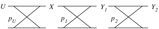
Figure 2: The physically degraded BSBC. $p_{U}$, $p_{1}$ and $p_{2}$ are the transition probabilities at the left, middle and right segments respectively.

For this channel, theorem 1 implies that $||\mathcal{U}||=2$. Due to the symmetry of the channel, the probability distribution of $U$ which maximizes the rates, is a symmetric binary distribution, $\Pr(U=0)=\Pr(U=1)=\frac{1}{2}$. The resulting capacity region for this case is depicted in figure 3 for the case where $R_{0}=0$. In the figure, the bottom line (dash) is the non-cooperative capacity region, and the top line (dash-dot) is the maximum possible sum rate, which requires that $C_{12}\geq h(p_{12})-h(p_{1})$, where

$$h(p) = -p\log_{2}(p)-(1-p)\log_{2}(1-p),$$

$$p_{12} = p_{1}(1-p_{2})+p_{2}(1-p_{1}).$$

This maximum sum-rate of $I(X;Y_{1})$ is obtained by summing the rate to $R_{x1}$ given by (23) and the maximum possible rate for $R_{x2}$ given by (25), and using the Markov chain relation $U-X-Y_{1}$.

Figure 3: The capacity region for the physically degraded BSBC. Top, middle and bottom lines correspond to maximum possible cooperation, partial cooperation and no-cooperation scenarios respectively.

The middle line (solid) is the capacity region for the partial cooperation case where $0<C_{12}<h(p_{12})-h(p_{1})$.

As can be seen from this example, the capacity region derived in this section is strictly larger than the capacity region for the non-cooperation case. Indeed, summing the constraints on $R_{0}$, $R_{1}$ and $R_{2}$ without cooperation (equations (5), (6)), results in a maximum achievable sum-rate of

$$R_{0}+R_{1}+R_{2}\leq I(X;Y_{1})-(I(U;Y_{1})-I(U;Y_{2})),$$ (26)

where the second term is always positive due to the Markov chain $U-X-Y_{1}-Y_{2}$ (assuming the degrading channel is non-invertible). In this setup, the maximum possible sum-rate, $I(X;Y_{1})$, is achieved only when $U$ is a constant, and thus no information is sent to $R_{x2}$. When $R_{0}+R_{2}>0$, because of the relationship $R_{0}+R_{2}\leq I(U;Y_{2})<I(U;Y_{1})$, we cannot achieve the maximum sum-rate of $I(X;Y_{1})$ to $R_{x1}$. However, summing (24) or (25) with (23), results in a maximum achievable sum-rate with cooperating receivers of

$$R_{0}+R_{1}+R_{2}\leq I(X;Y_{1})$$

$$\phantom{xxxxxxx}+\min\left\{0,C_{12}-(I(U;Y_{1})-I(U;Y_{2}))\right\}.$$ (27)

Comparing this to non-cooperative sum-rate given by (26), it is clear that cooperation allows a net increase in the sum-rate, by at most $C_{12}$.

IV Achievable Rates for the General Broadcast Channel with Cooperating Receivers

For the classic general BC scenario, the best achievability result was derived by Marton in [14]. This result states that for the general BC, any rate pair $(R_{1},R_{2})$ satisfying

$$R_{1} \leq I(U;Y_{1}),$$ (28)

$$R_{2} \leq I(V;Y_{2}),$$ (29)

$$R_{1}+R_{2} \leq I(U;Y_{1})+I(V;Y_{2})-I(U;V),$$ (30)

for some joint distribution $p(u,v,x,y_{1},y_{2})=p(u,v,x)p(y_{1},y_{2}|x)$, is achievable.

We note that Marton’s largest region contains three auxiliary RVs, $(W,U,V)$, where $W$ represents information decoded by both receivers. Here we use a simplified version, where $W$ is set to a constant.

We now consider cooperation between the receivers. We begin with a statement of the theorem:

Theorem 2

Let $\left(\mathcal{X},p(y_{1},y_{2}|x),\mathcal{Y}_{1}\times\mathcal{Y}_{2}\right)$ be any discrete memoryless broadcast channel, with cooperating receivers having noiseless conference links of finite capacities $C_{12}$ and $C_{21}$, as defined in Section II. Then, for sending independent information, any rate pair $\left(R_{1},R_{2}\right)$ satisfying

$$R_{1} \leq R(U),$$

$$R_{2} \leq R(V),$$

$$R_{1}+R_{2} \leq R(U)+R(V)-I(U;V),$$

subject to,

$$C_{21} \geq I(\hat{U};Y_{2})-I(\hat{U};Y_{1}),$$ (31)

$$C_{12} \geq I(\hat{V};Y_{1})-I(\hat{V};Y_{2}),$$ (32)

where,

$$R(U) = I(U;Y_{1},\hat{U}),$$ (33)

$$R(V) = I(V;Y_{2},\hat{V}),$$ (34)

for some joint distribution $p(u,v,x,y_{1},y_{2},\hat{u},\hat{v})=p(u,v,x)p(y_{1},y_{2}|x)p(\hat{u}|y_{2})p(\hat{v}|y_{1})$, is achievable, with $u\in\mathcal{U},v\in\mathcal{V},\hat{u}\in\mathcal{\hat{U}},\hat{v}\in\mathcal{\hat{V}}$, $||\mathcal{\hat{U}}||\leq||\mathcal{Y}_{2}||+1$ and $||\mathcal{\hat{V}}||\leq||\mathcal{Y}_{1}||+1$.

In the next subsections we provide the proof of this theorem.

IV-A Overview of Coding Strategy

As in the achievability part of theorem 1, the proposed code is a hybrid broadcast-relay code. Here, we combine the relay code construction of [34, theorem 6] and the broadcast code construction of [15]. The fact that in these two theorems the channel encoding and the relay operation are performed independently, allows to easily combine them into a hybrid coding scheme. The encoder generates broadcast codewords, each selected from a codebook constructed similarly to the construction of [15]. This codebook splits the rate between the two users. Next, each relay ($R_{x1}$ acts as a relay for $R_{x2}$ and vice-versa) generates its codebook according to the construction of [34, theorem 6]. In the decoding step, using the received signal ($Y_{1}^{n}$ at $R_{x1}$ and $Y_{2}^{n}$ at $R_{x2}$), each receiver generates a list of the possible transmitted relay messages and uses the conference message from the next time interval to resolve for the relay massage. Then, each receiver uses the decoded relay message and its received channel output to decode its own message.

IV-B Encoding at the Transmitter

1. Let $\epsilon>0$ and $n\geq 1$ be given. Fix $p(u,v,x)$, $p(\hat{u}|y_{2})$ and $p(\hat{v}|y_{1})$, and let $\delta>0$ be a positive number, whose selection is described in the next item. Let $A_{\delta}^{*(n)}(U)$ denote the set of strongly typical i.i.d. sequences of length $n$, ${\bf u}\in\mathcal{U}^{n}$, as defined in [43, Ch. 13.6]. Let $A_{\delta}^{*(n)}(V)$ denote the set of strongly typical i.i.d. sequences of length $n$, ${\bf v}\in\mathcal{V}^{n}$. Let $S_{[U]\delta}^{(n)}$ denote the set of all sequences ${\bf u}\in A_{\delta}^{*(n)}(U)$, such that $A_{\delta}^{*(n)}(V|{\bf u})$ is nonempty as defined in [47, corollary 5.11], and similarly define $S_{[V]\delta}^{(n)}$ for the sequences ${\bf v}\in A_{\delta}^{*(n)}(V)$.

2. Select $2^{n\left(R(U)-\epsilon\right)}$ strongly typical sequences ${\bf u}$ in an i.i.d. manner, according to the probability

   $$p\left({\bf u}\right)=\left\{\begin{array}[]{cl}\frac{1}{||S_{[U]\delta}^{(n)}||}&,{\bf u}\in S_{[U]\delta}^{(n)}\\ 0&,\mbox{otherwise}.\end{array}\right.$$

   Label these sequences by ${\bf u}(k),\;k\in\Big{[}1,2^{n\left(R(U)-\epsilon\right)}\Big{]}$. Select $2^{n\left(R(V)-\epsilon\right)}$ strongly typical sequences ${\bf v}$ in an i.i.d. manner, according to the probability

   $$p\left({\bf v}\right)=\left\{\begin{array}[]{cl}\frac{1}{||S_{[V]\delta}^{(n)}||}&,{\bf v}\in S_{[V]\delta}^{(n)}\\ 0&,\mbox{otherwise}.\end{array}\right.$$

   Label these sequences by ${\bf v}(l),\;l\in\left[1,2^{n\left(R(V)-\epsilon\right)}\right]$. Note that from [47, corollary 5.11] we have that $||S_{[U]\delta}^{(n)}||\geq(1-\delta)2^{n(H(U)-\psi)}$, where $\psi\rightarrow 0$ as $n\rightarrow\infty$ and $\delta\rightarrow 0$, so for any $\epsilon>0$ we can always find $0<\delta\leq\epsilon$ such that for $n$ large enough we obtain $||S_{[U]\delta}^{(n)}||>2^{n\left(I\left(U;Y_{1},\hat{U}\right)-\epsilon\right)}$ and $||S_{[V]\delta}^{(n)}||>2^{n\left(I\left(V;Y_{2},\hat{V}\right)-\epsilon\right)}$.

3. Define the cells $B_{i}=\left[(i-1)2^{n\left(R(U)-R_{1}-\epsilon\right)}+1,i2^{n\left(R(U)-R_{1}-\epsilon\right)}\right]$, $i\in\left[1,2^{nR_{1}}\right]$. This is a partition of the ${\bf u}$ sequences into $2^{nR_{1}}$ sets. Define the cells
   $C_{j}=\left[(j-1)2^{n\left(R(V)-R_{2}-\epsilon\right)}+1,j2^{n\left(R(V)-R_{2}-\epsilon\right)}\right]$, $j\in\left[1,2^{nR_{2}}\right]$, which form a partition of the ${\bf v}$ sequences into $2^{nR_{2}}$ sets.

4. For every pair of integers $(w_{1},w_{2})\in\left[1,2^{nR_{1}}\right]\times\left[1,2^{nR_{2}}\right]$, define the set $\mathcal{D}_{w_{1},w_{2}}=\Big{\{}\left({\bf u}(k),{\bf v}(l)\right):k\in B_{w_{1}},l\in C_{w_{2}},\left.\left({\bf u}(k),{\bf v}(l)\right)\in A_{\epsilon}^{*(n)}(U,V)\right\}.$ Here, $A_{\epsilon}^{*(n)}(U,V)$ denotes the strongly typical set for the random variables $U$ and $V$ as defined in [43, Ch. 13.6]. In the following we may omit the random variables when referring to the strongly typical set, when these variables are clear from the context. We now have the following (slightly modified) lemma from [15]:

   Lemma 1

   For any 2-D cell $B_{i}\times C_{j}$, $\epsilon>0$, and $n$ large enough, we have that $\mbox{Pr}\left(||\mathcal{D}_{ij}||=0\right)\leq\epsilon$, provided that

   $$\!\!\!\!\!\!\!\!\!\!R_{1}+R_{2} < R(U)+R(V)-I(U;V)-2\epsilon-\epsilon_{1},$$ (37)

   where $\epsilon_{1}\rightarrow 0$ as $\epsilon\rightarrow 0$ and $n\rightarrow\infty$.

   Proof:

   The proof of this lemma is obtained by direct application of the technique used to prove [15, Lemma in pg. 121], and therefore will not be repeated here. ∎

5. For each message pair $(w_{1},w_{2})$, select one pair $({\bf u}(k_{w_{1},w_{2}}),{\bf v}(l_{w_{1},w_{2}}))\in\mathcal{D}_{w_{1},w_{2}}$. For each of the selected pairs (one pair for each message pair), generate a codeword according to ${\bf x}(w_{1},w_{2})\sim\prod_{i=1}^{n}p\left(x_{i}|u_{i}(k_{w_{1},w_{2}}),v_{i}(l_{w_{1},w_{2}})\right)$.

6. To transmit the message pair $(w_{1},w_{2})$ the transmitter outputs ${\bf x}(w_{1},w_{2})$.

IV-C Encoding the Relay Messages

Consider first the relay encoding at $R_{x2}$, which acts as a relay for $R_{x1}$.

1. $R_{x2}$-relay has a set of $2^{nC_{21}}$ relay messages indexed by $s^{\prime}\in\left[1,2^{nC_{21}}\right]$. For each index $s^{\prime}$, generate $2^{nR^{\prime}}$ i.i.d. sequences $\hat{{\bf u}}$, each with probability $p(\hat{{\bf u}})=\prod_{i=1}^{n}p(\hat{u}_{i})$,
   $p(\hat{u})=\sum_{\mathcal{X},\mathcal{Y}_{1},\mathcal{Y}_{2}}p(\hat{u}|y_{2})p(y_{1},y_{2}|x)p(x)$, and $p(x)=\sum_{\mathcal{U},\mathcal{V}}p(u,v,x)$. Label these codewords $\hat{{\bf u}}(z^{\prime}|s^{\prime})$, $s^{\prime}\in\left[1,2^{nC_{21}}\right]$, $z^{\prime}\in[1,2^{nR^{\prime}}]$.

2. Randomly and uniformly partition the message set $[1,2^{nR^{\prime}}]$ into $2^{nC_{21}}$ sets $S^{\prime}_{s^{\prime}}$, $s^{\prime}\in\left[1,2^{nC_{21}}\right]$.

3. Encoding: Assume that after receiving ${\bf y}_{2}(i-1)$ we have at $R_{x2}$ that $\left(\hat{{\bf u}}(z_{i-1}^{\prime}|s_{i-1}^{\prime}),{\bf y}_{2}(i-1)\right)\in A_{\epsilon}^{*(n)}$, and that $z_{i-1}^{\prime}\in S^{\prime}_{s_{i}^{\prime}}$ ($s_{i-1}^{\prime}$ is known from the previous transmission of $z_{i-2}^{\prime}$). Then, at the $i$’th transmission interval the relay transmits the index $s_{i}^{\prime}$ to $R_{x1}$.

Relay encoding at $R_{x1}$ is performed in a symmetric manner to the relay encoding at $R_{x2}$. The corresponding variables for $R_{x1}$ are $S^{\prime\prime}_{s^{\prime\prime}}$ and $\hat{{\bf v}}(z^{\prime\prime}|s^{\prime\prime})$, $s^{\prime\prime}\in\left[1,2^{nC_{12}}\right]$, $z^{\prime\prime}\in[1,2^{nR^{\prime\prime}}]$.

IV-D Decoding the Relay Messages at the Relays

Consider decoding the relay message at $R_{x2}$. The relay decoder at $R_{x2}$ uses its channel input ${\bf y}_{2}(i)$, and its previously decoded $s_{i}^{\prime}$ to generate the relay message $z_{i}^{\prime}$ as follows: upon receiving ${\bf y}_{2}(i)$, the relay $R_{x2}$ decides that the message $z_{i}^{\prime}$ was received at time $i$ if $\left(\hat{{\bf u}}\left(z_{i}^{\prime}|s_{i}^{\prime}\right),{\bf y}_{2}(i)\right)\in A_{\epsilon}^{*(n)}$. Following the argument in [34, theorem 6] (see also the proof in [43, Ch. 13.6]), there exists such $z_{i}^{\prime}$ with probability that is arbitrarily close to one as long as

$$R^{\prime}\geq I\left(\hat{U};Y_{2}\right),$$ (38)

and $n$ is sufficiently large. Relay decoding at $R_{x1}$ is done in a symmetric manner to the relay decoding at $R_{x2}$.

IV-E Decoding at the Receivers

We first find the rate constraint for decoding at $R_{x1}$. $R_{x1}$ decodes its message $w_{1,i-1}$ based on its channel input ${\bf y}_{1}(i-1)$ and the relay indices $s_{i}^{\prime}$ and $s_{i-1}^{\prime}$:

1. From knowledge of $s_{i-1}^{\prime}$ and ${\bf y}_{1}(i-1)$, $R_{x1}$ calculates the set $\mathcal{L}_{1}(i-1)$ such that

   $$\mathcal{L}_{1}(i-1) = \Big{\{}z^{\prime}\in[1,2^{nR^{\prime}}]:$$

   $$\qquad\left(\hat{{\bf u}}\left(z^{\prime}|s_{i-1}^{\prime}\right),{\bf y}_{1}(i-1)\right)\in A_{\epsilon}^{*(n)}\Big{\}}.$$

2. At the time interval of the $i$’th codeword, $R_{x1}$ receives the relayed $s_{i}^{\prime}$. Since $s_{i}^{\prime}$ is selected from a set of $2^{nC_{21}}$ possible messages, it can be transmitted over the noiseless conference link without error.

3. $R_{x1}$ now chooses $\hat{z}_{i-1}^{\prime}$ as the relay message at time $i-1$ if and only if there exists a unique $\hat{z}_{i-1}^{\prime}\in S^{\prime}_{s_{i}^{\prime}}\bigcap\mathcal{L}_{1}(i-1)$. Again, following the reasoning in [34, theorem 6], this can be done with an arbitrarily small probability of error as long as

   $$R^{\prime}\leq I(\hat{U};Y_{1})+C_{21},$$ (39)

   and $n$ is large enough. Combining this with inequality (38) we get the constraint on the relay information rate:

   $$C_{21}\geq I(\hat{U};Y_{2})-I(\hat{U};Y_{1}).$$ (40)

   This expression is similar to the Wyner-Ziv expression for the rate required to transmit $Y_{2}$ to receiver $R_{x1}$ up to a given distortion, determined by $p(\hat{u}|y_{2})$ and a decoder. Here the performance of the decoder are implied in the mutual information $I(U;Y_{1},\hat{U})$. The compressed $Y_{2}^{n}$ is then used by $R_{x1}$ to assist in decoding $W_{1}$.

4. Lastly, $R_{x1}$ decodes $w_{1,i-1}$ (or, equivalently ${\bf u}(k_{w_{1,i-1},w_{2,i-1}})$) by choosing ${\bf u}(k_{\hat{w}_{1,i-1},\hat{w}_{2,i-1}})$ such that $\left({\bf u}(k_{\hat{w}_{1,i-1},\hat{w}_{2,i-1}}),{\bf y}_{1}(i-1),\hat{{\bf u}}\left(\hat{z}_{i-1}^{\prime}|s_{i-1}^{\prime}\right)\right)\in A_{\epsilon}^{*(n)}$. From the point-to-point channel coding theorem (see [15]) we have that $\hat{w}_{1,i-1}=w_{1,i-1}$ with probability that is arbitrarily close to one, as long as $z_{i-1}^{\prime}$ was correctly decoded at $R_{x1}$ and

   $$R_{1}\leq R(U)\triangleq I\left(U;Y_{1},\hat{U}\right),$$ (41)

   for sufficiently large $n$. Combining this with equation (40) yields the rate constraint on $R_{1}$:

   $$R_{1} \leq R(U),$$ (43)

   $$\mbox{as long as }C_{21}\geq I(\hat{U};Y_{2})-I(\hat{U};Y_{1}).$$

Using symmetric arguments to those presented for decoding at $R_{x1}$ we find the rate constraint for $R_{x2}$ to be

$$R_{2} \leq R(V),$$ (45)

$$\mbox{as long as }C_{12}\geq I(\hat{V};Y_{1})-I(\hat{V};Y_{2}).$$

Combining equations (37), (43), (43), (45) and (45), gives the conditions in theorem 2.

IV-F Error Events

In the scheme described above we have to account for the following error events for decoding $(w_{1,i-1},w_{2,i-1})$:

1. Encoding at the transmitter fails:
   $E_{D,i}=\left\{||\mathcal{D}_{w_{1,i-1},w_{2,i-1}}||=0\right\}$.

2. Joint typicality decoding fails:
   $E_{0,i}=\Big{\{}\big{(}{\bf u}(k_{w_{1,i-1},w_{2,i-1}}),{\bf v}(l_{w_{1,i-1},w_{2,i-1}}),$xxxxxxxx
   xxxxx${\bf x}(w_{1,i-1},w_{2,i-1}),{\bf y}_{1}(i-1),{\bf y}_{2}(i-1)\big{)}\notin A_{\epsilon}^{*(n)}\Big{\}}$.

3. Decoding at the relays fails: $E_{1,i}=E_{11,i}\bigcup E_{12,i}$,
   $E_{11,i}=\Big{\{}\nexists z^{\prime}\in[1,2^{nR^{\prime}}]\;\mbox{s.t.}$ xxxxxxxxxxxxxxxx
   xxxxxxxxxxx $\;\left(\hat{{\bf u}}\left(z^{\prime}|s_{i-1}^{\prime}\right),{\bf y}_{2}(i-1)\right)\in A_{\epsilon}^{*(n)}\Big{\}}$,
   $E_{12,i}=\Big{\{}\nexists z^{\prime\prime}\in[1,2^{nR^{\prime\prime}}]\;\mbox{s.t.}$ xxxxxxxxxxxxxxxx
   xxxxxxxxxxx $\;\left(\hat{{\bf v}}\left(z^{\prime\prime}|s_{i-1}^{\prime\prime}\right),{\bf y}_{1}(i-1)\right)\in A_{\epsilon}^{*(n)}\Big{\}}$.

4. Decoding the relay message at the receivers fails: $E_{2,i}=E_{21,i}\bigcup E_{22,i}$, where $E_{21,i}=E_{21,i}^{\prime}\bigcup E_{21,i}^{\prime\prime}$ and $E_{22,i}=E_{22,i}^{\prime}\bigcup E_{22,i}^{\prime\prime}$,
   $E_{21,i}^{\prime}=\left\{z_{i-1}^{\prime}\notin S^{\prime}_{s_{i}^{\prime}}\bigcap\mathcal{L}_{1}(i-1)\right\}$,
   $E_{21,i}^{\prime\prime}=\left\{\exists\tilde{z}^{\prime}\neq z_{i-1}^{\prime}\;\mbox{s.t.}\;\tilde{z}^{\prime}\in S^{\prime}_{s_{i}^{\prime}}\bigcap\mathcal{L}_{1}(i-1)\right\}$,
   $E_{22,i}^{\prime}=\left\{z_{i-1}^{\prime\prime}\notin S^{\prime\prime}_{s_{i}^{\prime\prime}}\bigcap\mathcal{L}_{2}(i-1)\right\}$,
   $E_{22,i}^{\prime\prime}=\left\{\exists\tilde{z}^{\prime\prime}\neq z_{i-1}^{\prime\prime}\;\mbox{s.t.}\;\tilde{z}^{\prime\prime}\in S^{\prime\prime}_{s_{i}^{\prime\prime}}\bigcap\mathcal{L}_{2}(i-1)\right\}$,
   $\mathcal{L}_{2}(i-1)\triangleq\Big{\{}z^{\prime\prime}\in[1,2^{nR^{\prime\prime}}]:$xxxxxxxxxxxxxxxx
   xxxxxxxxxxxxx $\left(\hat{{\bf v}}\left(z^{\prime\prime}|s_{i-1}^{\prime\prime}\right),{\bf y}_{2}(i-1)\right)\in A_{\epsilon}^{*(n)}\Big{\}}$.

5. Final decoding at the receivers fails:
   $E_{3,i}=E_{31,i}\bigcup E_{32,i}$, where,
   $E_{31,i}=\Big{\{}\big{(}{\bf u}(k_{w_{1,i-1},w_{2,i-1}}),{\bf y}_{1}(i-1),$xxxxxxxxx $\hat{{\bf u}}(z_{i-1}^{\prime}|s_{i-1}^{\prime})\big{)}\notin A_{\epsilon}^{*(n)}\Big{\}}$ $\!\!\!\bigcup\Big{\{}\exists w_{1}\neq w_{1,i-1}\;\mbox{s.t.}$ $\phantom{XXX}\left({\bf u}(k_{w_{1},w_{2}}),{\bf y}_{1}(i-1),\hat{{\bf u}}(z_{i-1}^{\prime}|s_{i-1}^{\prime})\right)\in A_{\epsilon}^{*(n)}\Big{\}}$,
   $E_{32,i}=\Big{\{}\big{(}{\bf v}(l_{w_{1,i-1},w_{2,i-1}}),{\bf y}_{2}(i-1),$xxxxxxxxx $\hat{{\bf v}}(z_{i-1}^{\prime\prime}|s_{i-1}^{\prime\prime})\big{)}\notin A_{\epsilon}^{*(n)}\Big{\}}$ $\!\!\!\bigcup\Big{\{}\exists w_{2}\neq w_{2,i-1}\;\mbox{s.t.}$ $\phantom{XXX}\left({\bf v}(l_{w_{1},w_{2}}),{\bf y}_{2}(i-1),\hat{{\bf v}}(z_{i-1}^{\prime\prime}|s_{i-1}^{\prime\prime})\right)\in A_{\epsilon}^{*(n)}\Big{\}}$.

We now bound the probability of the error events at time $i$. Note that at time $i$ both $R_{x1}$ and $R_{x2}$ share the same $s_{i-1}^{\prime}$ and $s_{i-1}^{\prime\prime}$ irrespective whether the decoding at the relays was correct at time $i-1$. Hence, a decoding error at time $i-1$ does not affect the decoding at time $i$. Now, from lemma 1 it follows that by taking $n$ large enough the probability of $E_{D,i}$ can be made arbitrarily small, as long as (37) is satisfied. Additionally, by taking $n$ large enough, the probability $\Pr(E_{0,i}\bigcap E_{D,i}^{c})$ can be made arbitrarily small by the properties of strongly typical sequences, see [43, lemma 13.6.2]. The probability $\Pr(E_{1,i})$ can be made arbitrarily small as long as (43) and (45) are satisfied, as explained is section IV-D. Next, the Markov lemma [50, lemma 4.2] and the Markov chains $Y_{1}-Y_{2}-\hat{U}$ and $Y_{2}-Y_{1}-\hat{V}$, imply that $\Pr(E_{21,i}^{\prime}\bigcap E_{1,i}^{c}\bigcap E_{0,i}^{c})$ and $\Pr(E_{22,i}^{\prime}\bigcap E_{1,i}^{c}\bigcap E_{0,i}^{c})$ can be made arbitrarily small by taking $n$ large enough, and $\Pr(E_{21,i}^{\prime\prime}\bigcap E_{i,1}^{c})$ and $\Pr(E_{22,i}^{\prime\prime}\bigcap E_{i,1}^{c})$ can be made arbitrarily small by taking $n$ large enough as long as (43) and (45) are satisfied. Finally, $\Pr(E_{31,i}\bigcap E_{2,i}^{c}\bigcap E_{1,i}^{c}\bigcap E_{0,i}^{c}\bigcap E_{D,i}^{c})$ and $\Pr(E_{32,i}\bigcap E_{2,i}^{c}\bigcap E_{1,i}^{c}\bigcap E_{0,i}^{c}\bigcap E_{D,i}^{c})$ can be made arbitrarily small by taking $n$ large enough by the Markov lemma and the chains $U,Y_{1}-Y_{2}-\hat{U}$ and $V,Y_{2}-Y_{1}-\hat{V}$, and as long as (43) and (45) are satisfied.

This concludes the proof of theorem 2. $\blacksquare$

IV-G An Upper Bound

Proposition 1

Assume the broadcast channel setup of theorem 2. Then, for sending independent information, any achievable rate pair $(R_{1},R_{2})$ must satisfy

$$R_{1} \leq I(X;Y_{1})+C_{21},$$

$$R_{2} \leq I(X;Y_{2})+C_{12},$$

$$R_{1}+R_{2} \leq I(X;Y_{1},Y_{2}),$$

for some distribution $p(x)$ on $\mathcal{X}$.

Proof:

The proof uses the cut-set bound [43, theorem 14.10.1]. First we define an equivalent system by introducing two orthogonal channels $X_{2}^{\prime}-Y_{1}^{\prime}$ from $R_{x2}$ to $R_{x1}$ and $X_{1}^{\prime}-Y_{2}^{\prime}$ from $R_{x1}$ to $R_{x2}$. The joint probability distribution function then becomes

$$p\left((y_{1},y_{1}^{\prime}),(y_{2},y_{2}^{\prime})|x,x_{1}^{\prime},x_{2}^{\prime}\right)=p(y_{1},y_{2}|x)p(y_{1}^{\prime}|x_{2}^{\prime})p(y_{2}^{\prime}|x_{1}^{\prime}),$$

where the signal received at $R_{x1}$ is $(Y_{1},Y_{1}^{\prime})$ and the signal received at $R_{x2}$ is $(Y_{2},Y_{2}^{\prime})$. As in the proof in section III-A3, we select $\mathcal{X}_{1}^{\prime}$, $\mathcal{X}_{2}^{\prime}$, $\mathcal{Y}_{1}^{\prime}$, $\mathcal{Y}_{2}^{\prime}$, $p(x_{1}^{\prime})$, $p(x_{2}^{\prime})$, $p(y_{1}^{\prime}|x_{2}^{\prime})$ and $p(y_{2}^{\prime}|x_{1}^{\prime})$ such that the capacities of the channels $X_{2}^{\prime}-Y_{1}^{\prime}$ and $X_{1}^{\prime}-Y_{2}^{\prime}$ are $C_{21}$ and $C_{12}$ respectively. Additionally, the codewords for the conference transmissions are determined independently from the source codebook so we set $p(x,x_{1}^{\prime},x_{2}^{\prime})=p(x)p(x_{1}^{\prime})p(x_{2}^{\prime})$. Now, from the cut-set bound, letting the transmitter and $R_{x2}$ form one group and $R_{x1}$ the second group, we have

$$R_{1} \leq I(X,X_{2}^{\prime};Y_{1},Y_{1}^{\prime}|X_{1}^{\prime})$$

$$= I(X_{2}^{\prime};Y_{1},Y_{1}^{\prime}|X_{1}^{\prime})+I(X;Y_{1},Y_{1}^{\prime}|X_{1}^{\prime},X_{2}^{\prime})$$

$$= I(X_{2}^{\prime};Y_{1}^{\prime}|X_{1}^{\prime})+I(X_{2}^{\prime};Y_{1}|X_{1}^{\prime},Y_{1}^{\prime})$$

$$\phantom{xxxxxx}+I(X;Y_{1}^{\prime}|X_{1}^{\prime},X_{2}^{\prime})+I(X;Y_{1}|X_{1}^{\prime},X_{2}^{\prime},Y_{1}^{\prime})$$

$$= I(X_{2}^{\prime};Y_{1}^{\prime})+I(X;Y_{1})$$

$$= C_{21}+I(X;Y_{1}),$$

where $I(X_{2}^{\prime};Y_{1}|X_{1}^{\prime},Y_{1}^{\prime})=I(X;Y_{1}^{\prime}|X_{1}^{\prime},X_{2}^{\prime})=0$ follows from direct application of the distribution function. Similarly we obtain the rate constraint on $R_{2}$. Lastly, for the sum-rate consider the transmitter in one group and the receivers in the second. Then, the cut-set bound results in

$$R_{1}+R_{2} \leq I(X;Y_{1},Y_{2},Y_{1}^{\prime},Y_{2}^{\prime}|X_{1}^{\prime},X_{2}^{\prime})$$

$$= I(X;Y_{1},Y_{2}|X_{1}^{\prime},X_{2}^{\prime})$$

$$\phantom{xxxxxxxx}+I(X;Y_{1}^{\prime},Y_{2}^{\prime}|X_{1}^{\prime},X_{2}^{\prime},Y_{1},Y_{2})$$

$$= I(X;Y_{1},Y_{2}),$$

yielding the last constraint in the proposition. ∎

IV-H Remarks

Comment IV.1

Observing the rate constraints in theorem 2 we can see that when (31) and (32) are satisfied then the cooperative rates are greater than the non-cooperative rates due to the (generally) positive terms adding to $I(U;Y_{1})$ and $I(V;Y_{2})$.

Comment IV.2

We note that although we present a single letter characterization of the rates, we are not able to apply standard cardinality bounding techniques such as those used in [48] or [49] for bounding $||\mathcal{U}||$ and $||\mathcal{V}||$. The method of [48] cannot be applied since it relies on the fact that the auxiliary random variables are independent, which is not the case here. The method of [49] cannot be applied as explained in the comment for theorem 2 in [20]. The cardinality bounds on $||\mathcal{\hat{U}}||$ and $||\mathcal{\hat{V}}||$ are trivial since they are transmitted over noiseless links.

Comment IV.3

The relay strategies can be divided into two general classes. The first class is referred to as decode-and-forward (DAF). In this strategy, the relay first decodes the message intended for the destination and then generates a relay message based on the decoded information. The second class is referred to as estimate-and-forward (EAF). In this class the relay does not decode the message intended for the destination but transmits an estimate of its channel input to the destination. For the physically degraded BC we used DAF, based on [34, theorem 1], to derive theorem 1, and for the general BC we used the EAF scheme of [34, theorem 6], to derive theorem 2. Of course, one can also combine both strategies and perform partial decoding at each receiver of the other receiver’s message before conferencing, following [34, theorem 7]. This combination will, in general, result in an increased achievable rate region.

IV-I Special Cases

IV-I1 No Cooperation: $C_{12}=C_{21}=0$

Consider first cooperation from $R_{x2}$ to $R_{x1}$. Setting $C_{21}=0$ in theorem 2 implies that

$$H(\hat{U}|Y_{1})=H(\hat{U}|Y_{2}).$$ (46)

From equation (33), the constraint on $R_{1}$ can be written in the form

$$R_{1} \leq I(U;Y_{1})+I(U;\hat{U}|Y_{1}).$$

Now we find $I(U;\hat{U}|Y_{1})$:

$$I(U;\hat{U}|Y_{1}) = H(\hat{U}|Y_{1})-H(\hat{U}|Y_{1},U)$$

$$\stackrel{{\scriptstyle(a)}}{{=}} H(\hat{U}|Y_{2})-H(\hat{U}|Y_{1},U)$$

$$\stackrel{{\scriptstyle(b)}}{{=}} H(\hat{U}|Y_{2},Y_{1},U)-H(\hat{U}|Y_{1},U)$$

$$= -I(\hat{U};Y_{2}|Y_{1},U).$$

where (a) is due to (46), and (b) is due to the Markov chain $U-(U,V)-X-(Y_{1},Y_{2})-Y_{2}-\hat{U}$, which implies that given $Y_{2}$, $\hat{U}$ is independent of $Y_{1}$ and $U$. Now, since mutual information is non-negative, we conclude that $I(U;\hat{U}|Y_{1})=0$. Hence, the rate constraint on $R_{1}$ becomes

$$R_{1}\leq I(U;Y_{1}).$$

Similarly, the maximum rate $R_{2}$ is given by $I(V;Y_{2})$, and in conclusion when $C_{12}=C_{21}=0$ we resort back to the rate region without cooperation derived in [14] (with a constant $W$).

IV-I2 Full Cooperation: $C_{12}=H(Y_{1}|Y_{2})$, $C_{21}=H(Y_{2}|Y_{1})$

When $C_{12}=H(Y_{1}|Y_{2})$, we get from (32) that

$$H(Y_{1}|Y_{2})=C_{12} \geq I(\hat{V};Y_{1})-I(\hat{V};Y_{2})$$

$$= H(\hat{V}|Y_{2})-H(\hat{V}|Y_{1}),$$

which is satisfied when $\hat{V}=Y_{1}$. Plugging this into (34), we get that when full cooperation from $R_{x1}$ to $R_{x2}$ is available, the rate constraint for $R_{x2}$ becomes

$$R_{2}\leq I(V;Y_{2},Y_{1}).$$

Using the same reasoning we conclude that when full cooperation from $R_{x2}$ to $R_{x1}$ is available, the rate constraint for $R_{x1}$ becomes $R_{1}\leq I(U;Y_{1},Y_{2})$.

IV-I3 Partial Cooperation

When $0<C_{12}<H(Y_{1}|Y_{2})$ and $0<C_{21}<H(Y_{2}|Y_{1})$, we get that

$$C_{21} \geq H(\hat{U}|Y_{1})-H(\hat{U}|Y_{2})$$

$$\Rightarrow H(\hat{U}|Y_{1}) \leq C_{21}+H(\hat{U}|Y_{2}).$$ (48)

Hence, the achievable rate to $R_{x1}$ is upper bounded by

$$R_{1} \leq I(U;Y_{1},\hat{U})$$

$$= I(U;Y_{1})+I(U;\hat{U}|Y_{1})$$

$$= I(U;Y_{1})+H(\hat{U}|Y_{1})-H(\hat{U}|U,Y_{1})$$

$$\stackrel{{\scriptstyle(a)}}{{\leq}} I(U;Y_{1})+H(\hat{U}|Y_{2})-H(\hat{U}|U,Y_{1})+C_{21}$$

$$\stackrel{{\scriptstyle(b)}}{{=}} I(U;Y_{1})+H(\hat{U}|Y_{2},Y_{1},U)-H(\hat{U}|U,Y_{1})+C_{21}$$

$$R_{1} \leq I(U;Y_{1})+C_{21}-I(\hat{U};Y_{2}|U,Y_{1}).$$ (49)

where (a) is due to (48) and (b) follow from the same reasoning leading to equation (IV-I1). Similarly, $R_{2}\leq I(V;Y_{2})+C_{12}-I(\hat{V};Y_{1}|V,Y_{2})$.

Note that there exist negative terms $-I(\hat{U};Y_{2}|U,Y_{1})$ and $-I(\hat{V};Y_{1}|V,Y_{2})$ in the achievable rate upper bounds. This can be explained as follows: the mutual information $I(\hat{U};Y_{2}|U,Y_{1})$ can be considered as a type of “ancillary” information that $\hat{U}$ contains, since this information is contained in $\hat{U}$ while $U$ and $Y_{1}$ are already known - therefore, this information is a “noise” part of $Y_{2}$ which does not include any helpful information for decoding $U$ at $R_{x1}$. Thus, for cooperating in the optimal way, $\hat{U}$ has to be a type of “sufficient and complete” cooperation information.

V The General Broadcast Channel with a Single Common Message

We now consider the case where only a single message, rather than two independent messages, is transmitted to both receivers. The main motivation for considering this case is that in the two independent messages case it is difficult to specify an explicit cooperation scheme, and we therefore have to represent cooperation through auxiliary random variables. Hence, we cannot identify directly the gain from cooperation, except in the case of full cooperation, and we also cannot evaluate the achievable region. For the single common message case, we are able to derive results for partial cooperation without auxiliary variables, which make this region explicitly computable. This scenario is depicted in figure 4.

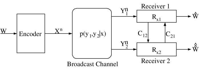
Figure 4: The single message broadcast channel with cooperating receivers. $\hat{W}$ and $\hat{\hat{W}}$ are the estimates of $W$ at $R_{x1}$ and $R_{x2}$ respectively.

For this scenario we need to specialize the definitions of a code and the average probability of error as follows:

• A $\left(2^{nR},n,(C_{12},C_{21})\right)$ code for sending a common message over the broadcast channel with cooperating receivers having conference links of capacities $C_{12}$ and $C_{21}$ between them, is defined in a similar manner to definition 6 with $\mathcal{W}_{1}$, $\mathcal{W}_{2}$ and $\mathcal{W}_{1}\times\mathcal{W}_{2}$ all replaced with $\mathcal{W}=\left\{1,2,...,2^{nR}\right\}$.

• The average probability of error is defined similarly to definition 7 with $W_{1}$ and $W_{2}$ replaced with $W$.

The capacity for the non-cooperative single message scenario is given in [5] by

$$C=\sup_{p(x)}\Big{\{}\min\big{(}I(X;Y_{1}),I(X;Y_{2})\big{)}\Big{\}}.$$ (50)

In the following we consider two cooperation schemes, referred to as a single-step scheme and a two-step scheme. These schemes are described in figure 5. In the single-step scheme, after reception each receiver generates a single cooperation message based on its channel input. In the two-step scheme, after reception one receiver generates a cooperation message based only on its channel input, as in the previous case, but the second receiver generates its cooperation message only after decoding (which is done with the help of the conference message from the first receiver). In both cases each receiver generates a single conference message, however in the single-step conference the emphasis is on low delay, while in the two-step conference we sacrifice delay in order to gain rate.

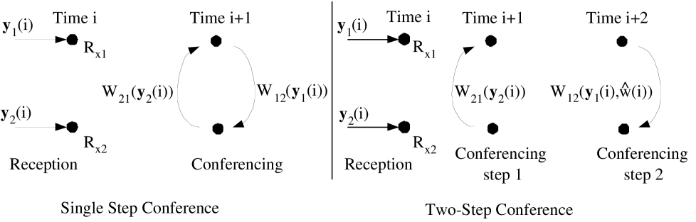
Figure 5: Schematic description of the single-step and the two-step conference schemes.

V-A Decoding with a Single-Step Cooperation

In this section we constrain both decoders to output their decoded messages after a conference that consists of a single message from each receiver, based only on its received channel input. For this case, we can specialize the derivation of theorem 2 and get the following achievable rate for the broadcast channel with partially cooperating receivers:

Theorem 3

Let $\left(\mathcal{X},p(y_{1},y_{2}|x),\mathcal{Y}_{1}\times\mathcal{Y}_{2}\right)$ be any discrete memoryless broadcast channel, with cooperating receivers having noiseless conference links of finite capacities $C_{12}$ and $C_{21}$, as defined in section II. Then, for sending a common message to both receivers, any rate $R$ satisfying

$$R \leq \sup_{p(x)}\Big{\{}\min\big{\{}I(X;Y_{1},\hat{U}),I(X;Y_{2},\hat{V})\big{\}}\Big{\}},$$

subject to

$$C_{21} \geq I(\hat{U};Y_{2})-I(\hat{U};Y_{1}),$$

$$C_{12} \geq I(\hat{V};Y_{1})-I(\hat{V};Y_{2}),$$

for some joint distribution $p(x,y_{1},y_{2},\hat{u},\hat{v})=p(x)p(y_{1},y_{2}|x)p(\hat{u}|y_{2})p(\hat{v}|y_{1})$ is achievable, with $||\mathcal{\hat{U}}||\leq||\mathcal{Y}_{2}||+1$ and $||\mathcal{\hat{V}}||\leq||\mathcal{Y}_{1}||+1$.

The proof of theorem 3 follows the same lines of the proof of theorem 2 and will not be repeated here. We next show how we can increase the rates by introducing the two-step conference.

V-B Decoding with a Two-Step Cooperation

We consider a two-step conference: at the first step only one receiver decodes the message. The second receiver decodes after the second step. Therefore, after the first receiver decodes the message, relaying to the second receiver reduces to the decode-and-forward relay situation of [34, theorem 1]. The rates achievable with a two step conference are given in the following theorem:

Theorem 4

Assume the broadcast channel setup of theorem 3. Then, for sending a common message to both receivers, any rate $R$ satisfying

$$R \leq \sup_{p(x)}\Bigg{[}\max\Big{\{}R^{12}(p(x)),R^{21}(p(x))\Big{\}}\Bigg{]}$$

$$R^{12}(p(x)) \triangleq \min\bigg{(}I(X;Y_{1})+C_{21},$$

$$\qquad I(X;Y_{2})-I(\hat{V};Y_{1}|Y_{2},X)$$

$$\qquad+\min\big{(}C_{12},H(\hat{V}|Y_{2})-H(\hat{V}|Y_{1})\big{)}\bigg{)},$$

$$R^{21}(p(x)) \triangleq \min\bigg{(}I(X;Y_{2})+C_{12},$$

$$\qquad I(X;Y_{1})-I(\hat{U};Y_{2}|Y_{1},X)$$

$$\qquad+\min\big{(}C_{21},H(\hat{U}|Y_{1})-H(\hat{U}|Y_{2})\big{)}\bigg{)},$$

for some joint distribution $p(x,y_{1},y_{2},\hat{u},\hat{v})=p(x)p(y_{1},y_{2}|x)p(\hat{u}|y_{2})p(\hat{v}|y_{1})$ is achievable, with $||\mathcal{\hat{U}}||\leq||\mathcal{Y}_{2}||+1$ and $||\mathcal{\hat{V}}||\leq||\mathcal{Y}_{1}||+1$, and with the appropriate $C_{12}\geq I(\hat{V};Y_{1}|Y_{2},X)$ or $C_{21}\geq I(\hat{U};Y_{2}|Y_{1},X)$ (the one used for the first cooperation step).

Proof:

V-B1 Overview of Coding Strategy

The scheme described in theorem 3 uses a single-step conference for both decoders. However, if we let one receiver use a two-step conference, then that receiver, instead of using conference information derived from the raw input of the other receiver, can use information generated by the second receiver after it already decoded the message. This conference information is less noisy, and thus the rate to the first receiver can be increased.

To put this in more concrete terms, assume that at time $i+1$, $R_{x1}$ sends to $R_{x2}$ the index $s^{\prime}_{i+1}$ of the partition into which its relay message at time $i$, denoted $z_{\hat{v},i}$, belongs. In appendix B we show that $R_{x2}$ can decode the message $w_{0,i}$ with an arbitrarily small probability of error as long as

$$R \leq I(X;Y_{2})-I(\hat{V};Y_{1}|Y_{2},X)$$ (51)

$$\qquad+\min\left(C_{12},H(\hat{V}|Y_{2})-H(\hat{V}|Y_{1})\right),$$

and

$$C_{12}\geq I(\hat{V};Y_{1}|Y_{2},X).$$ (52)

We now introduce the following modifications to the scheme used in theorem 3:

V-B2 Relay Sets Generation at $R_{x2}$

$R_{x2}$ partitions the message set $\mathcal{W}$ into $2^{nC_{21}}$ subsets in a uniform and independent manner. Denote these subsets with $\widetilde{S}^{\prime\prime}_{\widetilde{s}^{\prime\prime}},\>\widetilde{s}^{\prime\prime}\in\left[1,2^{nC_{21}}\right]$.

V-B3 Relay Encoding at $R_{x2}$

$R_{x2}$ has an estimate $\hat{\hat{w}}_{0,i}$ of the message $w_{0,i}$. Now, $R_{x2}$ looks for the partition into which $\hat{\hat{w}}_{0,i}$ belongs and sends the index of this partition, denoted $\widetilde{s}^{\prime\prime}_{i+2}$, to $R_{x1}$ at time $i+2$.

V-B4 Decoding at $R_{x1}$

Upon reception of ${\bf y}_{1}(i)$, $R_{x1}$ generates the set $\mathcal{L}_{1}(i)=\left\{w\in\mathcal{W}:\left({\bf x}(w),{\bf y}_{1}(i)\right)\in A_{\epsilon}^{*(n)}(X,Y_{1})\right\}$. At time $i+2$, upon reception of $\widetilde{s}^{\prime\prime}_{i+2}$, $R_{x1}$ looks for an index $w$ such that $w\in\mathcal{L}_{1}(i)\bigcap\widetilde{S}^{\prime\prime}_{\widetilde{s}^{\prime\prime}_{i+2}}$. If a unique such $w$ exists then $R_{x1}$ sets $\hat{w}_{0,i}=w$, otherwise an error is declared.

V-B5 Bounding the Probability of Error

Using the proof technique in [34, theorem 1], it can be easily shown that assuming correct decoding at $R_{x2}$, then any rate $R\leq I(X;Y_{1})+C_{21}$ is achievable to $R_{x1}$.

Combining the bounds derived above, we conclude that with a two-step conference at $R_{x1}$, any rate satisfying

$$R \leq \min\bigg{(}I(X;Y_{1})+C_{21},I(X;Y_{2})-I(\hat{V};Y_{1}|Y_{2},X)$$

$$\qquad\qquad+\min\big{(}C_{12},H(\hat{V}|Y_{2})-H(\hat{V}|Y_{1})\big{)}\bigg{)},$$

$$C_{12} \geq I(\hat{V};Y_{1}|Y_{2},X),$$

ia achievable. Repeating the same derivation when $R_{x2}$ uses a two-step conference, and combining with the previous case proves theorem 4. ∎

Setting $\hat{U}=Y_{2}$, $\hat{V}=Y_{1}$ in theorem 4 we obtain the following achievable region:

Corollary 1

Assume the broadcast channel setup of theorem 3. Then, for sending a common message to both receivers, any rate $R$ satisfying

$$R \leq \sup_{p(x)}\Bigg{[}\max\Big{\{}R^{12}(p(x)),R^{21}(p(x))\Big{\}}\Bigg{]}$$

$$R^{12}(p(x))\!\! \triangleq \!\!\min\bigg{(}\!I(X;Y_{1})+C_{21},I(X;Y_{2})-H(Y_{1}|Y_{2},X)$$

$$\phantom{xxxxxxx}+\min\big{(}C_{12},H(Y_{1}|Y_{2})\big{)}\bigg{)},$$

$$R^{21}(p(x))\!\! \triangleq \!\!\min\bigg{(}\!I(X;Y_{2})+C_{12},I(X;Y_{1})-H(Y_{2}|Y_{1},X)$$

$$\phantom{xxxxxxx}+\min\big{(}C_{21},H(Y_{2}|Y_{1})\big{)}\bigg{)},$$

with the appropriate $C_{12}>H(Y_{1}|Y_{2},X)$ or $C_{21}>H(Y_{2}|Y_{1},X)$ (the one used for the first cooperation step), is achievable.

This gives a partial cooperation result without auxiliary random variables.

V-C An Example for Corollary 1

Consider two independent, identical, BSBCs with transition probability $p$, and cooperation links of capacities $C_{12}=C_{21}=C$. For this case, corollary 1 gives the following maximum achievable rate:

$$R = \sup_{p_{0}}\bigg{\{}\min\Big{[}H(Y_{1})-h(p)+C,$$

$$\qquad\qquad\quad\min\left(H(Y_{1})+C,H(Y_{1},Y_{2})\right)-2h(p)\Big{]}\bigg{\}},$$

$$= \sup_{p_{0}}\bigg{\{}\min\Big{[}H(Y_{1})-2h(p)+C,H(Y_{1},Y_{2})-2h(p)\Big{]}\bigg{\}},$$

for $C\geq h(p)$, where $\mathcal{Y}_{1}=\mathcal{Y}_{2}=\mathcal{X}=\left\{0,1\right\}$, $p_{0}=\Pr(X=0)$, and

$$\Pr(y_{1},y_{2}) = \left\{\begin{array}[]{cl}(1-p)^{2}p_{0}+p^{2}(1-p_{0}),&y_{1}=y_{2}=0\\ p(1-p),&y_{1}\neq y_{2}\\ p^{2}p_{0}+(1-p)^{2}(1-p_{0}),&y_{1}=y_{2}=1\end{array}\right.$$

$$\Pr(y_{1}) = \left\{\begin{array}[]{cl}(1-p)p_{0}+p(1-p_{0}),&y_{1}=0\\ pp_{0}+(1-p)(1-p_{0}),&y_{1}=1.\end{array}\right.$$

Solving for the supremum for each value of $C$, we get the achievable rates depicted in figure 6.

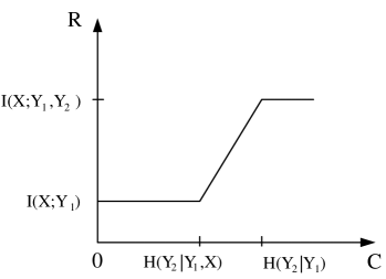
Figure 6: Achievable rate vs. C, for the two independent, identical, BSBCs with a single common message, resulting from corollary 1.

Note the linear increase in the achievable rate for $H(Y_{2}|Y_{1},X)<C<H(Y_{2}|Y_{1})$.

V-D An Upper Bound

The upper bound for the single common message case can be obtained from the bound for the two independent messages case in proposition 1:

Corollary 2

Let $\left(\mathcal{X},p(y_{1},y_{2}|x),\mathcal{Y}_{1}\times\mathcal{Y}_{2}\right)$ be any discrete memoryless broadcast channel, with cooperating receivers having noiseless conference links of finite capacities $C_{12}$ and $C_{21}$, as defined in section II. Then, for sending a common message to both receivers, any rate $R$ must satisfy

$$R \leq \sup_{p(x)}\Big{\{}\min\big{(}I(X;Y_{1})+C_{21},I(X;Y_{2})+C_{12},$$

$$\qquad\qquad\qquad I(X;Y_{1},Y_{2})\big{)}\Big{\}}.$$

Proof:

Follows directly from proposition 1 by noting that the common rate has to satisfy all three constraints: the individual rates and the sum rate. ∎

V-E Remarks

Comment V.1

Note that there are special cases where the lower bound of corollary 1 coincides with the upper bound of corollary 2, yielding the capacity for these cases. For example, assume a strong version of the “more capable” condition of [5]: $I(X;Y_{1})>>I(X;Y_{2})$ for all input distributions $p(x)$ on $\mathcal{X}$ . Assume also that $H(Y_{2}|Y_{1},X)<C_{21}<H(Y_{2}|Y_{1})$ and $H(Y_{1}|Y_{2},X)<C_{12}<H(Y_{1}|Y_{2})$. Under these conditions, we have that $I(X;Y_{1})+C_{21}>I(X;Y_{2})+C_{12}-H(Y_{1}|Y_{2},X)$. Thus, if $R_{x1}$ is helping $R_{x2}$ first, the achievable rate is $I(X;Y_{2})+C_{12}-H(Y_{1}|Y_{2},X)$. If $R_{x2}$ is helping $R_{x1}$ first, then the achievable rate is $I(X;Y_{2})+C_{12}$. Since $C_{12}-H(Y_{1}|Y_{2},X)<C_{12}$, this cooperation scheme achieves the upper bound $R=\sup_{p(x)}\left\{I(X;Y_{2})+C_{12}\right\}$.

Comment V.2

Note that the capacity region for the deterministic broadcast channel with cooperating receivers follows from corollary 1 and corollary 2. This region was derived in [51]. For this case we have that $H(Y_{1}|X)=H(Y_{2}|X)=0$ hence $I(X;Y_{i})=H(Y_{i})$, $i=1,2$. The achievable rate (from corollary 1) is given by

$$R \leq \min\left\{H(Y_{2})+C_{12},H(Y_{1})+\min\left(C_{21},H(Y_{2}|Y_{1})\right)\right\}$$

$$= \min\left\{H(Y_{2})+C_{12},H(Y_{1})+C_{21},H(Y_{1},Y_{2})\right\},$$

and the same from corollary 2.

Comment V.3

We note that although the expressions in (51) and (52) seem different from the EAF expression of [34, theorem 6], given in theorem 3 (cf. $R\leq I(X;Y_{2},\hat{V}),\mbox{ subject to }C_{12}\geq I(\hat{V};Y_{1})-I(\hat{V};Y_{2})$), this does not improve on the achievable rate of the standard EAF. The reason is that every rate achievable according to (51)-(52) can also be achieved with the standard EAF using the same mapping of the auxiliary RV and an appropriate time-sharing. However, when considering a specific, fixed assignment of the auxiliary random variable (such as in corollary 1) then the rate achievable with (51)-(52) is indeed greater than the classic EAF with the same assignment.

VI Conclusions

In this paper we investigated the effect of cooperation between receivers on the rates for the broadcast channel. As communication networks evolve, it can be expected that in future networks, nodes that are close enough to be able to communicate directly, will use this ability to help each other in reception. Accommodating this characteristic, we extended the traditional broadcast scenario, in which each decoder is assumed to operate independently, into a scenario where the receivers have finite capacity links used for cooperation. We analyzed three related scenarios: the physically degraded BC - for which we derived the capacity region, the general BC for which we presented an achievability result, and the single common message case. For the last case we identified a special case where capacity can be achieved. We note that it is not trivial to extend these results to more than two steps, since the intermediate steps need to extract information from partial relay information. Although this can be done by introducing additional auxiliary variables, obtaining a computable region is not a simple task. This study is an initial step in this investigation and future work includes several extensions: a natural first extension is to consider a fully wireless system, and extend the analysis to the Gaussian case. Another extension is to consider the interaction between the Wyner-Ziv compression and the achievable rates for the general channel.

Appendix A Background Results

Consider the construction in section III-A. Let $\mathcal{L}(i-1)=\left\{w_{2}:\left({\bf y}_{2}(i-1),{\bf u}(w_{2}|s_{i-1})\right)\in A_{\epsilon}^{(n)}\right\}$. We bound $E_{{\bf y}_{2}}\left\{||\mathcal{L}(i-1)||\right\}$. Let,

$$\psi\left(w_{2}\left|{\bf y}_{2}(i-1)\right.\right)=\left\{\begin{array}[]{cc}1,&\left({\bf u}(w_{2}|s_{i-1}),{\bf y}_{2}(i-1)\right)\in A_{\epsilon}^{(n)}\\ 0,&\mbox{otherwise.}\end{array}\right.$$

Hence, as in [34, theorem 1], we can write the random variable $||\mathcal{L}(i-1)||$ as a sum of random variables:

$$||\mathcal{L}(i-1)||=\sum_{w_{2}=1}^{2^{nR_{2}}}\psi\left(w_{2}\left|{\bf y}_{2}(i-1)\right.\right),$$

and therefore

$$E_{{\bf y}_{2}}\Big{\{}||\mathcal{L}(i-1)||\Big{\}} = E_{{\bf y}_{2}}\left\{\psi\left(w_{2,i-1}\left|{\bf y}_{2}(i-1)\right.\right)\right\}$$

$$\phantom{x}+\!\!\!\sum_{\begin{subarray}{c}w_{2}=1\\ w_{2}\neq w_{2,i-1}\end{subarray}}^{2^{nR_{2}}}E_{{\bf y}_{2}}\left\{\psi\left(w_{2}\left|{\bf y}_{2}(i-1)\right.\right)\right\}.$$

When $w_{2}\neq w_{2,i-1}$ we get from the properties of independent sequence ([43, theorem 8.6.1]) that

$$E_{{\bf y}_{2}}\left\{\psi\left(w_{2}\left|{\bf y}_{2}(i-1)\right.\right)\right\} = \Pr\left\{\psi\left(w_{2}\left|{\bf y}_{2}(i-1)\right.\right)=1\right\}$$

$$\leq 2^{-n\left(I(U;Y_{2})-3\epsilon\right)},$$

thus,

$$E_{{\bf y}_{2}}\Big{\{}||\mathcal{L}(i-1)||\Big{\}}\leq 1+2^{nR_{2}}2^{-n\left(I(U;Y_{2})-3\epsilon\right)}.$$ (A.1)

Note that this result holds also when considering the strongly typical set rather than the weakly typical set.

Appendix B Proof of the Achievable Rate to the First Decoder in Theorem 4 (equations (51) and (52))

B-A Overview of Coding Strategy

The encoder generates a single codebook in a random and independent manner. Next, the first relay partitions its collection of relay codewords ($\mathcal{Z}(\hat{V})$ for $R_{x1}$) into disjoint sets. When a channel input is received, the first relay finds the index of the partition set which contains a relay codeword jointly typical with its channel input, and transmits it over the noiseless conference link to the second receiver. Then, the second receiver looks for a unique source codeword that is jointly typical with its channel input, and with at least one of the relay codewords in the set of possible codewords received from the first relay.

In the following analysis we assume that $R_{x1}$ is the first relay and $R_{x2}$ decodes first.

B-B Codebook Generation and Encoding at the Transmitter

Fix $p(x)$ and generate $2^{nR}$ i.i.d. codewords ${\bf x}$, with $p({\bf x}(w))=\prod_{i=1}^{n}p(x_{i}(w))$, $w\in\mathcal{W}=\left\{1,2,...,2^{nR}\right\}$. For transmitting the message $w_{0,i}$ at time $i$, the transmitter outputs ${\bf x}(w_{0,i})$ to the channel.

B-C Relay Sets Generation

Fix $p(\hat{v}|y_{1})$.

• Consider the p.d.f. $p(\hat{v})=\sum_{\mathcal{X},\mathcal{Y}_{1},\mathcal{Y}_{2}}p(\hat{v}|y_{1})p(y_{1},y_{2}|x)p(x)$ on $\mathcal{\hat{V}}$.

• $R_{x1}$ generates $2^{nR_{1}^{\prime}}$ $\hat{{\bf v}}$ sequences in an i.i.d. manner according to $p(\hat{{\bf v}}(z_{\hat{v}}))=\prod_{i=1}^{n}p(\hat{v}_{i}(z_{\hat{v}}))$, $z_{\hat{v}}\in\mathcal{Z}(\hat{V})=\left\{1,2,...,2^{nR_{1}^{\prime}}\right\}$.

• $R_{x1}$ partitions the message set $\mathcal{Z}(\hat{V})$ into $2^{nC_{12}}$ sets, by assigning an index between $\left[1,2^{nC_{12}}\right]$ to each $z_{\hat{v}}\in\mathcal{Z}(\hat{V})$, in a random, independent and uniform manner over $\left[1,2^{nC_{12}}\right]$. Denote these sets by $S^{\prime}_{s^{\prime}}$, $s^{\prime}\in\left[1,2^{nC_{12}}\right]$.

B-D Decoding and Encoding at the Relay ($R_{x1}$)

• Upon reception of ${\bf y}_{1}(i)$, the relay $R_{x1}$ decides that $z_{\hat{v},i}\in\mathcal{Z}(\hat{V})$ was received if $\left(\hat{{\bf v}}(z_{\hat{v},i}),{\bf y}_{1}(i)\right)\in A_{\epsilon}^{*(n)}(\hat{V},Y_{1})$. Now, $R_{x1}$ finds the index $s_{i+1}^{\prime}$ of the set $S_{s_{i+1}^{\prime}}^{\prime}$ s.t. $z_{\hat{v},i}\in S_{s_{i+1}^{\prime}}^{\prime}$. Then, at time $i+1$, $R_{x1}$ transmits $s_{i+1}^{\prime}$ to $R_{x2}$ through the finite capacity noiseless conference link. If there is no $z_{\hat{v}}\in\mathcal{Z}(\hat{V})$ such that $\hat{{\bf v}}(z_{\hat{v}})$ is jointly typical with ${\bf y}_{1}(i)$, an error is declared.

B-E Decoding the Source Message at $R_{x2}$

At the $i$’th transmission interval $R_{x2}$ generates the set $\mathcal{L}_{2}(i)=\left\{w\in\mathcal{W}:\left({\bf x}(w),{\bf y}_{2}(i)\right)\in A_{\epsilon}^{*(n)}(X,Y_{2})\right\}$. At the $(i+1)$’th transmission interval, $R_{x2}$ receives $s^{\prime}_{i+1}$ from $R_{x1}$ through the noiseless conference link. $R_{x2}$ then looks for a unique $\hat{w}_{0}$ s.t. $\hat{w}_{0}\in\mathcal{L}_{2}(i)$ and $\exists z_{\hat{v}}\in S^{\prime}_{s^{\prime}_{i+1}}$, for which $\left({\bf x}(\hat{w}_{0}),{\bf y}_{2}(i),\hat{{\bf v}}(z_{\hat{v}})\right)\in A_{\epsilon}^{*(n)}(X,Y_{2},\hat{V})$. If such unique $\hat{w}_{0}$ exists, then $\hat{w}_{0}$ is the decoded message at time $i$. If there is none, or there is more than one, an error is declared.

B-F Analysis of the Probability of Error

B-F1 Error Events

The error events for the scheme described above, for decoding the message $w_{0,i}$, are:

1. Relay decoding fails:
   $E_{0,i}=\Big{\{}\nexists z_{\hat{v}}\in\mathcal{Z}(\hat{V})\mbox{ s.t. }$ xxxxxxxxxxx
   xxxxxxxxxxxxxx $(\hat{{\bf v}}(z_{\hat{v}}),{\bf y}_{1}(i))\in A_{\epsilon}^{*(n)}(\hat{V},Y_{1})\Big{\}}$.

2. Joint typicality decoding fails: Let $E_{1,i}=E^{\prime}_{1,i}\bigcup E^{\prime\prime}_{1,i}$, where
   $E^{\prime}_{1,i}=\left\{\left({\bf x}(w_{0,i}),{\bf y}_{1}(i),{\bf y}_{2}(i)\right)\notin A_{\epsilon}^{*(n)}(X,Y_{1},Y_{2})\right\}$,
   $E^{\prime\prime}_{1,i}=\left\{\left({\bf x}(w_{0,i}),\hat{{\bf v}}(z_{\hat{v},i}),{\bf y}_{2}(i)\right)\notin A_{\epsilon}^{*(n)}(X,\hat{V},Y_{2})\right\}$.

3. Decoding at $R_{x2}$ fails: $E_{2,i}=E_{2,i}^{\prime}\bigcup E_{2,i}^{\prime\prime}$,
   $E_{2,i}^{\prime}=\Big{\{}\nexists z_{\hat{v}}\in S^{\prime}_{s^{\prime}_{i+1}}\;\mbox{for which}$xxxxxxxxxxxxxx
   xxxxxxxx $\;\left({\bf x}(w_{0,i}),\hat{{\bf v}}(z_{\hat{v}}),{\bf y}_{2}(i)\right)\in A_{\epsilon}^{*(n)}(X,\hat{V},Y_{2})\Big{\}},$
   $E_{2,i}^{\prime\prime}=\Big{\{}\exists w\neq w_{0,i},w\in\mathcal{L}_{2}(i)\;\mbox{s.t.}\;\exists z_{\hat{v}}\in S^{\prime}_{s^{\prime}_{i+1}},$xxxxx
   xxxxxxxxxx $\left({\bf x}(w),\hat{{\bf v}}(z_{\hat{v}}),{\bf y}_{2}(i)\right)\in A_{\epsilon}^{*(n)}(X,\hat{V},Y_{2})\Big{\}}$.

Next, applying the union bound we get that

$$P_{e}^{(n)} = \Pr\left(\bigcup_{k=0}^{2}E_{k,i}\right)$$

$$= \Pr(E_{0,i})+\Pr\left(E_{1,i}\bigcap E_{0,i}^{c}\right)$$

$$\phantom{xxxxxxxxx}+\Pr\left(E_{2,i}\bigcap E_{1,i}^{c}\bigcap E_{0,i}^{c}\right).$$

B-F2 Bounding the Probabilities of the Error Events

Following the same argument as in section IV-D, $R_{1}^{\prime}\geq I(\hat{V};Y_{1})$ implies that taking $n$ large enough, we can make $\Pr(E_{0,i})\leq\epsilon$. Next, from the properties of strongly typical sequences (see [43, lemma 13.6.1]), by taking $n$ large enough, we can make $\Pr(E^{\prime}_{1,i})\leq\frac{\epsilon}{2}$. Additionally, the Markov lemma, [50, lemma 4.2] implies that we can make $\Pr(E^{\prime\prime}_{1,i}\bigcap E_{1,i}^{\prime c}\bigcap E_{0,i}^{c})\leq\frac{\epsilon}{2}$ for any arbitrary $\epsilon>0$ by taking $n$ large enough. Therefore, by the union bound, $\Pr(E_{1,i}\bigcap E_{0,i}^{c})\leq\epsilon$. We also have that $\Pr(E^{\prime}_{2,i}\bigcap E_{1,i}^{c}\bigcap E_{0,i}^{c})=0$ because under $E_{1,i}^{c}\bigcap E_{0,i}^{c}$ we have that ${\bf x}(w_{0,i}),{\bf y}_{2}(i)$ and $\hat{{\bf v}}(z_{\hat{v},i})$ are jointly typical, and by construction, $z_{\hat{v},i}\in S^{\prime}_{s^{\prime}_{i+1}}$. Hence, we need to show that the probability $\Pr(E^{\prime\prime}_{2,i}\bigcap E_{1,i}^{c}\bigcap E_{0,i}^{c})$ can be made arbitrarily small. Note that due to the symmetry of the construction, the probability of error does not depend on the specific message $w_{0,i}$ transmitted.

B-F3 Bounding $\Pr(E^{\prime\prime}_{2,i}\bigcap E_{1,i}^{c}\bigcap E_{0,i}^{c})$

The probability of $E^{\prime\prime}_{2,i}\bigcap E_{1,i}^{c}\bigcap E_{0,i}^{c}$ can be written as

$$\Pr(E^{\prime\prime}_{2,i}\bigcap E_{1,i}^{c}\bigcap E_{0,i}^{c})$$

$$\;=\Pr\Big{(}\Big{\{}\exists z_{\hat{v}}\in S^{\prime}_{s^{\prime}_{i+1}},\exists w\neq w_{0,i},w\in\mathcal{L}_{2}(i),$$

$$\phantom{llll}\left({\bf x}(w),{\bf y}_{2}(i),\hat{{\bf v}}(z_{\hat{v}})\right)\in A_{\epsilon}^{*(n)}(X,Y_{2},\hat{V})\Big{\}}\bigcap E_{1,i}^{c}\bigcap E_{0,i}^{c}\Big{)}$$

$$\;\stackrel{{\scriptstyle(a)}}{{=}}\Pr\Big{(}\Big{\{}\exists w\neq w_{0,i},w\in\mathcal{L}_{2}(i),$$

$$\phantom{lll}\left({\bf x}(w),{\bf y}_{2}(i),\hat{{\bf v}}(z_{\hat{v},i})\right)\in A_{\epsilon}^{*(n)}(X,Y_{2},\hat{V})\Big{\}}\bigcap E_{1,i}^{c}\bigcap E_{0,i}^{c}\Big{)}$$

$$\phantom{xxx}+\Pr\Big{(}\Big{\{}\exists w\neq w_{0,i},w\in\mathcal{L}_{2}(i),\exists z_{\hat{v}}\in S^{\prime}_{s^{\prime}_{i+1}},z_{\hat{v}}\neq z_{\hat{v},i},$$

$$\phantom{xlll}\left({\bf x}(w),{\bf y}_{2}(i),\hat{{\bf v}}(z_{\hat{v}})\right)\in A_{\epsilon}^{*(n)}(X,Y_{2},\hat{V})\Big{\}}\bigcap E_{1,i}^{c}\bigcap E_{0,i}^{c}\Big{)}$$

$$\;\triangleq\Pr(E^{\prime\prime}_{2,1,i})+\Pr(E^{\prime\prime}_{2,2,i}),$$

where (a) is because the elements of $S^{\prime}_{s^{\prime}_{i+1}}$ are selected in an independent manner.

We first bound $\Pr\left(E_{2,1,i}^{\prime\prime}\right)$ as follows:

$$\Pr(E^{\prime\prime}_{2,1,i})=$$

$$\;\sum_{\mathcal{L}_{2}(i)}\Pr\Big{(}\Big{\{}\exists w\neq w_{0,i},w\in\mathcal{L}_{2}(i),\left({\bf x}(w),{\bf y}_{2}(i),\hat{{\bf v}}(z_{\hat{v},i})\right)$$

$$\qquad\quad\in A_{\epsilon}^{*(n)}(X,Y_{2},\hat{V})\Big{\}}\bigcap E_{1,i}^{c}\bigcap E_{0,i}^{c}\Big{|}\mathcal{L}_{2}(i)\Big{)}\Pr\left(\mathcal{L}_{2}(i)\right)$$

$$\stackrel{{\scriptstyle(a)}}{{\leq}}\;E_{{\bf y}_{2}}\Bigg{\{}\sum_{\begin{subarray}{c}w\in\mathcal{L}_{2}(i)\\ w\neq w_{0,i}\end{subarray}}\Pr\Big{(}\Big{\{}\left({\bf x}(w),{\bf y}_{2}(i),\hat{{\bf v}}(z_{\hat{v},i})\right)\in$$

$$\qquad\qquad\qquad\qquad A_{\epsilon}^{*(n)}(X,Y_{2},\hat{V})\Big{\}}\bigcap E_{1,i}^{c}\bigcap E_{0,i}^{c}\Big{|}{\bf y}_{2}(i)\Big{)}\Bigg{\}}$$

$$=E_{{\bf y}_{2}}\left\{\sum_{\begin{subarray}{c}w\in\mathcal{L}_{2}(i)\\ w\neq w_{0,i}\end{subarray}}\sum_{\begin{subarray}{c}\hat{{\bf v}}\in\\ A_{\epsilon}^{*(n)}(\hat{V}|{\bf y}_{2}(i),{\bf x}(w))\end{subarray}}\Pr\left(\hat{{\bf v}}|{\bf y}_{2}(i),{\bf x}(w)\right)\right\}$$

$$\stackrel{{\scriptstyle(b)}}{{=}}E_{{\bf y}_{2}}\left\{\sum_{\begin{subarray}{c}w\in\mathcal{L}_{2}(i)\\ w\neq w_{0,i}\end{subarray}}\sum_{\hat{{\bf v}}\in A_{\epsilon}^{*(n)}(\hat{V}|{\bf y}_{2}(i),{\bf x}(w))}\Pr\left(\hat{{\bf v}}|{\bf y}_{2}(i)\right)\right\}$$

$$\leq E_{{\bf y}_{2}}\Bigg{\{}\sum_{\begin{subarray}{c}w\in\mathcal{L}_{2}(i)\\ w\neq w_{0,i}\end{subarray}}||A_{\epsilon}^{*(n)}(\hat{V}|{\bf y}_{2}(i),{\bf x}(w))||\times$$

$$\qquad\qquad\qquad\qquad\max_{\begin{subarray}{c}\hat{{\bf v}}:\\ \left({\bf y}_{2}(i),\hat{{\bf v}}\right)\in A_{\epsilon}^{*(n)}(Y_{2},\hat{V})\end{subarray}}\Big{\{}\Pr\left(\hat{{\bf v}}|{\bf y}_{2}(i)\right)\Big{\}}\Bigg{\}}$$

$$\stackrel{{\scriptstyle(c)}}{{\leq}}E_{{\bf y}_{2}}\left\{\sum_{\begin{subarray}{c}w\in\mathcal{L}_{2}(i)\\ w\neq w_{0,i}\end{subarray}}2^{n(H(\hat{V}|Y_{2},X)+2\eta)}2^{-n\left(H(\hat{V}|Y_{2})-2\eta\right)}\right\}$$

$$\leq E_{{\bf y}_{2}}\left\{||\mathcal{L}_{2}(i)||\right\}2^{-n\left(H(\hat{V}|Y_{2})-H(\hat{V}|Y_{2},X)-4\eta\right)},$$

where (a) is because $\mathcal{L}_{2}(i)$ is a deterministic function of ${\bf y}_{2}(i)$ and we also applied the union bound and (b) is because $\hat{{\bf v}}(z_{\hat{v},i})$ is independent of ${\bf x}(w)$ for $w\neq w_{0,i}$. The bounds in (c) on the size of the conditionally typical set and the maximum conditional probability follow from [47, theorem 5.2] with $\eta\rightarrow 0$ as $\epsilon\rightarrow 0$, assuming that $n$ is large enough. Lastly we note that here

$$\Pr({\bf y}_{2}(i))\triangleq\Pr\left({\bf y}_{2}(i)\;\mbox{received}\;\big{|}\;{\bf x}(w_{0,i})\;\mbox{transmitted}\right).$$

Next, applying the same technique to bound the expectation of $||\mathcal{L}_{2}(i)||$ as in [34, theorem 1] (see also derivation of equation (A.1)), we get that for $n$ large enough,

$$E_{{\bf y}_{2}}\left\{||\mathcal{L}_{2}(i)||\right\}\leq 1+2^{n\left(R-I(X;Y_{2})+3\eta\right)}.$$ (B.1)

Plugging this back into the bound on $\Pr\left(E^{\prime\prime}_{2,1,i}\right)$ we get that

$$\!\!\!\!\!\!\!\!\!\!\!\!\Pr\left(E^{\prime\prime}_{2,1,i}\right) \leq 2^{-n\left(I\left(X;\hat{V}|Y_{2}\right)-4\eta\right)}$$ (B.2)

$$+2^{n\left(R-I(X;Y_{2})-H(\hat{V}|Y_{2})+H(\hat{V}|Y_{2},X)+7\eta\right)},$$

which can be made less than any arbitrary $\epsilon>0$ by taking $n$ large enough, as long as

$$R\leq I(X;Y_{2})-H(\hat{V}|Y_{2},X)+H(\hat{V}|Y_{2}).$$ (B.3)

For bounding $\Pr(E^{\prime\prime}_{2,2,i})$ we begin essentially in the same manner and get that

$$\!\!\!\!\!\!\!\!\Pr(E^{\prime\prime}_{2,2,i})$$

$$\stackrel{{\scriptstyle(a)}}{{\leq}} E_{{\bf y}_{2},\hat{{\bf v}}}\Bigg{\{}\Pr\left(\Big{\{}\exists w\neq w_{0,i},w\in\mathcal{L}_{2}(i),\exists z_{\hat{v}}\in S^{\prime}_{s^{\prime}_{i+1}},\right.$$

$$\qquad\qquad\qquad z_{\hat{v}}\neq z_{\hat{v},i},\left({\bf x}(w),{\bf y}_{2}(i),\hat{{\bf v}}(z_{\hat{v}})\right)\in$$

$$\qquad\qquad\qquad\qquad A_{\epsilon}^{*(n)}(X,Y_{2},\hat{V})\Big{\}}\Big{|}{\bf y}_{2}(i),\hat{{\bf v}}(z_{\hat{v},i})\Big{)}\Bigg{\}}$$

$$\stackrel{{\scriptstyle(b)}}{{\leq}} E_{{\bf y}_{2},\hat{{\bf v}}}\Bigg{\{}\sum_{\begin{subarray}{c}z_{\hat{v}}\in S^{\prime}_{s^{\prime}_{i+1}}\\ z_{\hat{v}}\neq z_{\hat{v},i}\end{subarray}}\sum_{\begin{subarray}{c}w\in\mathcal{L}_{2}(i)\\ w\neq w_{0,i}\end{subarray}}\Pr\Big{(}\left({\bf x}(w),{\bf y}_{2}(i),\hat{{\bf v}}(z_{\hat{v}})\right)\in$$

$$\qquad\qquad\qquad\qquad\quad A_{\epsilon}^{*(n)}(X,Y_{2},\hat{V})\Big{|}{\bf y}_{2}(i),\hat{{\bf v}}(z_{\hat{v},i})\Big{)}\Bigg{\}}$$

$$\stackrel{{\scriptstyle(c)}}{{=}} E_{{\bf y}_{2},\hat{{\bf v}}}\Bigg{\{}\sum_{\begin{subarray}{c}z_{\hat{v}}\in S^{\prime}_{s^{\prime}_{i+1}}\\ z_{\hat{v}}\neq z_{\hat{v},i}\end{subarray}}\sum_{\begin{subarray}{c}w\in\mathcal{L}_{2}(i)\\ w\neq w_{0,i}\end{subarray}}\sum_{\hat{{\bf v}}\in A_{\epsilon}^{*(n)}(\hat{V}|{\bf y}_{2}(i),{\bf x}(w))}\Pr\left(\hat{{\bf v}}\right)\Bigg{\}}$$

$$\stackrel{{\scriptstyle(d)}}{{\leq}} E_{\hat{{\bf v}}}\left\{||S^{\prime}_{s^{\prime}_{i+1}}||\right\}E_{{\bf y}_{2}}\left\{||\mathcal{L}_{2}(i)||\right\}2^{-n\left(H(\hat{V})-H(\hat{V}|Y_{2},X)-3\eta\right)}$$

$$\stackrel{{\scriptstyle(e)}}{{\leq}} \left(1+2^{n\left(R_{1}^{\prime}-C_{12}\right)}\right)\left(1+2^{n\left(R-I(X;Y_{2})+3\eta\right)}\right)\times$$

$$\qquad\qquad\qquad\qquad\qquad\quad\quad 2^{-n\left(H(\hat{V})-H(\hat{V}|Y_{2},X)-3\eta\right)}$$

$$\leq 2^{-n\left(C_{12}+H(\hat{V})-R_{1}^{\prime}-H(\hat{V}|Y_{2},X)-3\eta\right)}$$

$$\phantom{xx}+2^{n\left(R-I(X;Y_{2})-I(\hat{V};Y_{2},X)+6\eta\right)}+2^{-n\left(I(\hat{V};Y_{2},X)-3\eta\right)}$$

$$\;\phantom{XX}+2^{n\left(R-I(X;Y_{2})-C_{12}+R_{1}^{\prime}-H(\hat{V})+H(\hat{V}|Y_{2},X)+6\eta\right)},$$

where (a) is because we dropped the intersection with $E_{1,i}^{c}\bigcap E_{0,i}^{c}$, (b) is due to the union bound, (c) is because $\hat{{\bf v}}(z_{\hat{v}})$ is independent of ${\bf x}(w)$ and ${\bf y}_{2}(i)$ when $z_{\hat{v}}\neq z_{\hat{v},i}$, and (d) is because

$$E_{{\bf y}_{2},\hat{{\bf v}}}\big{\{}||\mathcal{L}_{2}(i)||\cdot||S^{\prime}_{s^{\prime}_{i+1}}||\big{\}}$$

$$\phantom{xxxxxxxxxxxx}=E_{{\bf y}_{2}}\Big{\{}E_{\hat{{\bf v}}|{\bf y}_{2}}\big{\{}||\mathcal{L}_{2}(i)||\cdot||S^{\prime}_{s^{\prime}_{i+1}}||\big{\}}\Big{\}}$$

$$\phantom{xxxxxxxxxxxx}\stackrel{{\scriptstyle(f)}}{{=}}E_{{\bf y}_{2}}\Big{\{}||\mathcal{L}_{2}(i)||E_{\hat{{\bf v}}|{\bf y}_{2}}\big{\{}||S^{\prime}_{s^{\prime}_{i+1}}||\big{\}}\Big{\}}$$

$$\phantom{xxxxxxxxxxxx}\stackrel{{\scriptstyle(g)}}{{=}}E_{{\bf y}_{2}}\Big{\{}||\mathcal{L}_{2}(i)||E_{\hat{{\bf v}}}\big{\{}||S^{\prime}_{s^{\prime}_{i+1}}||\big{\}}\Big{\}}$$

$$\phantom{xxxxxxxxxxxx}=E_{{\bf y}_{2}}\Big{\{}||\mathcal{L}_{2}(i)||\Big{\}}E_{\hat{{\bf v}}}\Big{\{}||S^{\prime}_{s^{\prime}_{i+1}}||\Big{\}},$$

where (f) is because the average size of $\mathcal{L}_{2}(i)$ does not depend on $\hat{{\bf v}}(z_{\hat{v},i})$ when ${\bf y}_{2}(i)$ is given, and (g) is because the average size of $S^{\prime}_{s^{\prime}_{i+1}}$ does not depend of ${\bf y}_{2}(i)$. The bounds on $\Pr(\hat{{\bf v}})$ and $||A_{\epsilon}^{*(n)}(\hat{V}|{\bf y}_{2},{\bf x})||$ in (d) follow from [47, Ch. 5]. The bound on $E_{{\bf y}_{2}}\left\{||\mathcal{L}_{2}(i)||\right\}$ in (e) follows from equation (B.1). We note that here

$$\!\!\!\!\!\Pr({\bf y}_{2}(i),\hat{{\bf v}}(z_{\hat{v},i}))\triangleq\Pr\Big{(}\left({\bf y}_{2}(i),\hat{{\bf v}}(z_{\hat{v},i})\right)\;\mbox{received}\;\big{|}\;{\bf x}(w_{0,i})$$

$$\phantom{xxxxxxxxxxxxxxxxxxxxxxxxxxxxxxxxx}\;\mbox{transmitted}\Big{)}.$$

We conclude that $\Pr\left(E_{2,2,i}^{\prime\prime}\right)$ can be made smaller than any $\epsilon>0$ by taking $n$ large enough, as long as

$$\!\!\!\!\!\!\!\!\!R \leq I(X;Y_{2})-H(\hat{V}|Y_{2},X)+C_{12}-R_{1}^{\prime}+H(\hat{V})$$ (B.4)

$$\!\!\!\!\!\!\!\!\!R_{1}^{\prime} \leq C_{12}-H(\hat{V}|Y_{2},X)+H(\hat{V})$$ (B.5)

$$\!\!\!\!\!\!\!\!\!R \leq I(X;Y_{2})+I(\hat{V};Y_{2},X)$$ (B.6)

$$\!\!\!\!\!\!\!\!\!R_{1}^{\prime} \geq I(\hat{V};Y_{1}),$$ (B.7)

where (B.7) follows from appendix B-F2.

Now note that making $\Pr(E^{\prime\prime}_{2,i}\bigcap E_{1,i}^{c}\bigcap E_{0,i}^{c})$ arbitrarily small requires making both $\Pr(E^{\prime\prime}_{2,1,i})$ and $\Pr(E^{\prime\prime}_{2,2,i})$ arbitrarily small. Thus we also need to satisfy (B.3). Combining with (B.6) we see that (B.3) guarantees (B.6) and we are left with (B.3), (B.4), (B.5) and (B.7).

The maximum rate is achieved for the minimal $R_{1}^{\prime}$, therefore we plug $R_{1}^{\prime}=I(\hat{V};Y_{1})$ in (B.4) and combining with (B.3) we obtain the following achievable rate

$$R \leq I(X;Y_{2})-H(\hat{V}|Y_{2},X)$$ (B.8)

$$\qquad\quad+\min\left(C_{12}+H(\hat{V}|Y_{1}),H(\hat{V}|Y_{2})\right).$$

From the combination of (B.5) and (B.7), we conclude that this is achievable as long as

$$C_{12} \geq I(\hat{V};Y_{1})+H(\hat{V}|Y_{2},X)-H(\hat{V})$$ (B.9)

$$= H(\hat{V}|Y_{2},X)-H(\hat{V}|Y_{1})$$

$$= I(\hat{V};Y_{1}|X,Y_{2}).$$

Equations (B.8) and (B.9) give the conditions for the message $W$ to be decoded at $R_{x2}$ with an arbitrarily small probability of error by taking $n$ large enough. Note that the requirement in (B.9) implies that when $C_{12}<I(\hat{V};Y_{1}|Y_{2},X)$, $R_{x1}$ cannot use this cooperation scheme, and the rate to $R_{x2}$ is simply $I(X;Y_{2})$. Combining this with equation (B.8) yields the rate expression in (51) and (52).

Ron Dabora received his B.Sc. and M.Sc. degrees in electrical engineering in 1994 and 2000 respectively, from Tel-Aviv University, Tel-Aviv, Israel. From 1994 to 2000, he was with the Signal Corps of Israel Defense Forces, and from 2000 to 2003, he was a member of the Algorithms Development Group, Millimetrix Broadband Networks, Israel. Since 2003 he is a Ph.D. student at Cornell University, Ithaca, NY.

Sergio D. Servetto was born in Argentina, on January 18, 1968. He received a Licenciatura en Informática from Universidad Nacional de La Plata (UNLP, Argentina) in 1992, and the M.Sc. degree in Electrical Engineering and the Ph.D. degree in Computer Science from the University of Illinois at Urbana-Champaign (UIUC), in 1996 and 1999. Between 1999 and 2001, he worked at the École Polytechnique Fédérale de Lausanne (EPFL), Lausanne, Switzerland. Since Fall 2001, he has been an Assistant Professor in the School of Electrical and Computer Engineering at Cornell University, and a member of the fields of Applied Mathematics and Computer Science. He was the recipient of the 1998 Ray Ozzie Fellowship, given to “outstanding graduate students in Computer Science,” and of the 1999 David J. Kuck Outstanding Thesis Award, for the best doctoral dissertation of the year, both from the Dept. of Computer Science at UIUC. He was also the recipient of a 2003 NSF CAREER Award. His research interests are centered around information theoretic aspects of networked systems, with a current emphasis on problems that arise in the context of large-scale sensor networks.

References

- [1] T. M. Cover. “Broadcast Channels”. IEEE Trans. Inform. Theory, IT-18(1):2–14, 1972.
- [2] P. P. Bergmans. “Random Coding Theorem for Broadcast Channels with Degraded Components”. IEEE Trans. Inform. Theory, IT-19(2):197–207, 1973.
- [3] P. P. Bergmans. “A Simple Converse for Broadcast Channels with Additive White Gaussian Noise”. IEEE Trans. Inform. Theory, IT-20(2):279–280, 1974.
- [4] R. G. Gallager. “Capacity and Coding for Degraded Broadcast Channels”. Problemy Peredachi Informatsii, vol. 10(3):3–14, 1974.
- [5] A. A. El Gamal. “The Capacity of a Class of Broadcast Channels”. IEEE Trans. Inform. Theory, IT-25(2):166–169, 1979.
- [6] A. A. El Gamal. “Broadcast Channels with and without Feedback”. Proc. 11th Annual Conf. on Circuits Systems and Computers, Pacific Grove, CA, 1978, pp. 180–183.
- [7] A. A. El Gamal. “The Capacity of the Physically Degraded Gaussian Broadcast Channel with Feedback”. IEEE Trans. Inform. Theory, IT-27(4):508–511, 1981.
- [8] A. A. El Gamal. “The Capacity of the Product and Sum of Two Unmatched Broadcast Channels”. Problemy Peredachi Informatsii, vol. 16(1):3–23, 1980.
- [9] T. S. Han. “The Capacity Region of the Deterministic Broadcast Channel with a Common Message”. IEEE Trans. Inform. Theory, IT-27(1):122–125, 1981.
- [10] M. Pinsker. “Capacity of Noiseless Broadcast Channels”. Problemy Peredachi Informatsii, vol. 14(2):28–34, 1978.
- [11] S. I. Gelfand. “Capacity of One Broadcast Channel”. Problemy Peredachi Informatsii, vol. 13(3):106–108, 1978.
- [12] T. M. Cover. “An Achievable Rate Region for the Broadcast Channel”. IEEE Trans. Inform. Theory, IT-21(4):399–404, 1975.
- [13] J. Korner and K. Marton. “General Broadcast Channels with Degraded Message Sets”. IEEE Trans. Inform. Theory, IT-23(1):60–64, 1977.
- [14] K. Marton. “A Coding Theorem for the Discrete Memoryless Broadcast Channel”. IEEE Trans. Inform. Theory, IT-25(3):306–311, 1979.
- [15] A. A. El Gamal and E. C. van der Meulen. “A Proof of Marton’s Coding Theorem for the Discrete Memoryless Broadcast Channel”. IEEE Trans. Inform. Theory, IT-27(1):120–122, 1981.
- [16] S. Vishwanath, G. Kramer, S. Shamai, S. Jafar, and A. Goldsmith. “Capacity Bounds for Gaussian Vector Broadcast Channels”. DIMACS Series in Multiantenna Channels: Capacity, Coding and Signal Processing, eds. G. J. Foschini and S. Verdu , vol. 62, pp. 107–122, 2003.
- [17] H. Sato. “An Outer Bound to the Capacity Region of Broadcast Channels”. IEEE Trans. Inform. Theory, IT-24(3):374–377, 1978.
- [18] L. H. Ozarow and S.K. Leung-Yan-Cheong. “An Achievable Region and Outer Bound for the Gaussian Broadcast Channel with Feedback”. IEEE Trans. Inform. Theory, IT-30(4):667–671, 1984.
- [19] N. Elia. “When Bode Meets Shannon: Control-Oriented Feedback Communication Schemes”. IEEE Trans. Autom. Control AC-49(9):1477–1487, 2004.
- [20] T. S. Han and M. H. M. Costa. “Broadcast Channels with Arbitrarily Correlated Sources”. IEEE Trans. Inform. Theory, IT-33(5):641–650, 1987.
- [21] T. M. Cover. “Comments on Broadcast Channels”. IEEE Trans. Inform. Theory, IT-44(6):2524–2530, 1998.
- [22] G. Caire and S. Shamai. “On the Achievable Throughtput of a Multiantenna Gaussian Broadcast Channel”. IEEE Trans. Inform. Theory, IT-49(7):1691–1705, 2003.
- [23] P. Viswanath and D.N.C. Tse. “Sum Capacity of the Vector Gaussian Broadcast Channel”. IEEE Trans. Inform. Theory, IT-49(8):1691–1705, 2003.
- [24] S. Vishwanath, N. Jindal and A. Goldsmith. “Duality, Achievable Rates, and Sum-Rate Capacity of Gaussian MIMO Broadcast Channels”. IEEE Trans. Inform. Theory, IT-49(10):2658–2668, 2003.
- [25] W. Yu and J. M. Cioffi. “Sum Capacity of Gaussian Vector Broadcast Channels”. IEEE Trans. Inform. Theory, IT-50(9):1875–1892, 2004.
- [26] H. Weingarten, Y. Steinberg, and S. Shamai. “The Capacity Region of the Gaussian MIMO Broadcast Channel”. Proc. IEEE Int. Symp. Inform. Theory (ISIT), Chicago, IL, 2004, p. 174.
- [27] S. C. Draper, B. J. Frey, and F. R. Kschischang. “Interactive Decoding of a Broadcast Message”. Proc. 41st Allerton Conf. on Communication, Control and Computing, Monticello, IL, 2003.
- [28] T. L. Willke and N. T. Maxemchuk. “Relieble Collaborative Decision Making in Moble Ad Hoc Networks”. Proc. 7th IFIP/IEEE Int. Conf. Management of Multimedia Networks and Services (MMNS), San Diego, CA, 2004.
- [29] E. C. van der Meulen. “Transmission of Information in a T-Terminal Discrete Memoryless Channel”. Ph.D. dissertation, Univ. California, Berkeley, 1968.
- [30] P. Gupta and P. R. Kumar. “The Capacity of Wireless Networks”. IEEE Trans. Inform. Theory, IT-46(2):388–404, 2000.
- [31] M. Gastpar and M. Vetterli. “On the Capacity of Large Gaussian Relay Networks”. IEEE Trans. Inform. Theory, IT-51(3):765–779, 2005.
- [32] P. Gupta and P. R. Kumar. “Towards an Information Theory of Large Networks: An Achievable Rate Region”. IEEE Trans. Inform. Theory, IT-49(8):1877–1894, 2003.
- [33] L. L. Xie and P. R. Kumar. “A Network Information Theory for Wireless Communication: Scaling Laws and Optimal Operation”. IEEE Trans. Inform. Theory, IT-50(5):748–767, 2004.
- [34] T. M. Cover and A. A. El Gamal. “Capacity Theorems for the Relay Channel”. IEEE Trans. Inform. Theory, IT-25(5):572–584, 1979.
- [35] B. Wang, J. Zhang and A. Host-Madsen. “On the Capacity of MIMO Relay Channels”. IEEE Trans. Inform. Theory, IT-51(1):29–43, 2005.
- [36] L. L. Xie and P. R. Kumar. “An Achievable Rate for the Multiple-Level Relay Channel”. IEEE Trans. Inform. Theory, IT-51(4):1348–1358, 2005.
- [37] G. Kramer, M. Gastpar and P. Gupta. “Cooperative Strategies and Capacity Theorems for Relay Networks”. IEEE Trans. Inform. Theory, IT-51(9):3037–3063, 2005.
- [38] H. F. Chong, M. Motani, and H. K. Garg. “New Coding Strategies for the Relay Channel”. In Proc. IEEE Int. Symp. Inform. Theory (ISIT), Adelaide, Australia, 2005, pp. 1086–1090.
- [39] R. Ahlswede, N. Cai, S.-Y. R. Li and R. W. Yeung. “Network Information Flow”. IEEE Trans. Inform. Theory, IT-46(4):1204–1216, 2000.
- [40] Z. Zhang. “Partial Converse for a Relay Channel”. IEEE Trans. Inform. Theory, IT-34(5):1106–1110, 1988.
- [41] A. D. Wyner and J. Ziv. “The Rate-Distortion Function for Source Coding with Side Information at the Decoder”. IEEE Trans. Inform. Theory, IT-22(1):1–10, 1976.
- [42] Y. Liang and V. V. Veeravalli. “The Impact of Relaying on the Capacity of Broadcast Channels”. Proc. IEEE Int. Symp. Inform. Theory (ISIT), Chicago, IL, 2004, p. 403.
- [43] T. M. Cover and J. Thomas. Elements of Information Theory. John Wiley and Sons Inc., 1991.
- [44] A. H. Kaspi. “Two-Way Source Coding with a Fidelity Criterion”. IEEE Trans. Inform. Theory, IT-31(6):735–740, 1985.
- [45] F. M. J. Willems. “The Discrete Memoryless Multiple Access Channel with Partially Cooperating Encoders”. IEEE Trans. Inform. Theory, IT-29(3):441–445, 1983.
- [46] R. Dabora and S. Servetto. “Broadcast Channels with Cooperating Receivers: a Downlink for the Sensor Reachback Problem”. Proc. IEEE Int. Symp. Inform. Theory (ISIT), Chicago, IL, 2004, p. 176.
- [47] R. W. Yeung. A First Course in Information Theory. Springer, 2002.
- [48] B. E. Hajek and M. B. Pursley. “Evaluation of an Achievable Rate Region for the Broadcast Channel”. IEEE Trans. Inform. Theory, IT-25(1):36–46, 1979.
- [49] M. Salehi. “Cardinality Bounds on Auxiliary Variables in Multiple-User Theory via the Method of Ahlswede and Korner”. Technical Report No. 33, Dept. Statistics, Stanford Univ., Stanford, CA, 1978.
- [50] T. Berger. Multiterminal Source Coding. The Information Theory Approach to Communictions, ed. G. Longo, Springer-Verlag, 1978.
- [51] S. C. Draper, B. J. Frey, and F. R. Kschischang. “On Interacting Encoders and Decoders in Multiuser Settings”. Proc. IEEE Int. Symp. Inform. Theory (ISIT), Chicago, IL, 2004, p. 118.