Defragmenting the Module Layout of a Partially Reconfigurable Device

Abstract

Modern generations of field-programmable gate arrays (FPGAs) allow for partial reconfiguration. In an online context, where the sequence of modules to be loaded on the FPGA is unknown beforehand, repeated insertion and deletion of modules leads to progressive fragmentation of the available space, making defragmentation an important issue. We address this problem by propose an online and an offline component for the defragmentation of the available space.

We consider defragmenting the module layout on a reconfigurable device. This corresponds to solving a two-dimensional strip packing problem. Problems of this type are NP-hard in the strong sense, and previous algorithmic results are rather limited. Based on a graph-theoretic characterization of feasible packings, we develop a method that can solve two-dimensional defragmentation instances of practical size to optimality. Our approach is validated for a set of benchmark instances.

Keywords: Reconfigurable computing, partial reconfiguration, defragmentation, two-dimensional packing, NP-hard problems, exact algorithms.

I Introduction

One of the cutting-edge aspects of modern reconfigurable computing is the possibility of partial reconfiguration of a device: Ideally, a new module can be placed on a reconfigurable chip whithout interfering with the processing of other running tasks. (See the end of this subsection for some pratical restrictions in current generations of FPGAs.) Clearly, this approach has many advantages over a full reconfiguration of the whole chip. Predominantly it lessens the bottleneck of reconfigurable computing: reconfiguration time.

On the other hand, partial reconfiguration introduces a new complexity: management of the free space on the FPGA. In the 2D model this is an NP-hard optimization problem. There has been a considerable amount of work to solve this problem computationally. However, due to its computational complexity most recent work has focused on the online setting or on the 1D area model (see [1] for a recent survey).

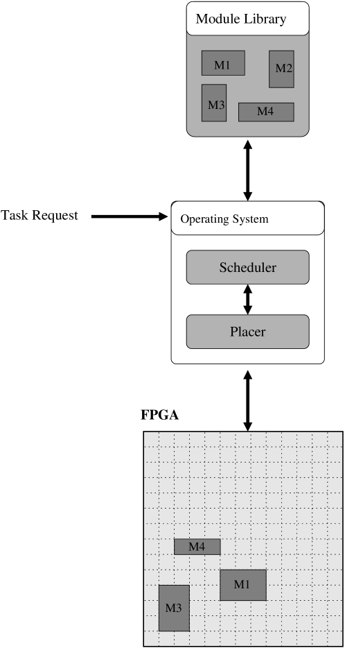
Figure 1: A schematic overview of an operating system for reconfigurable computers. Relocatable, presynthesized modules that are constrained to a rectangular layout are stored in a module library. As requests for tasks arrive, a module capable of running the task is selected, scheduled and eventually placed on the FPGA.

Management of free space and scheduling of arriving tasks are the core components of an operating system for reconfigurable platforms (see Figure 1). In all previous work these components use simple online strategies for the placement problem. The use of these strategies leads to fragmentation of the free space, as modules are placed on and removed from the chip area. This leads to situations where a new module has to be rejected by the placer because there is no free rectangle that could accomodate the new module even though the total free space available would be more than sufficient (see [2] for a discussion).

In this paper we propose a different placer module. Instead of just relying on online strategies our placer has an additional offline component: the defragmenter. Consider the following scenario: A car is equipped with a multimedia device that contains a partially reconfigurable FPGA. This multimedia device is responsible for audio, video, telephony and WLAN. While the car is in use, the device is busy and tasks must be scheduled and modules must be placed as they arrive. However, the recurring idle times of the car (i.e., over night) can be utilized to optimally defragment the FPGA chip area.

This optimal defragmentation follows two goals. One is to maximize the available contiguous free space. The other comes from the FPGA device we use. The current XILINX Virtex-II series does not admit full two-dimensional partial reconfiguration [3]. Instead, configuration can only be performed columnwise: While a column is reconfigured, all other modules that use this column have to be stopped, because reconfiguration interferes with the running tasks in a non-trivial way. So the other goal of the offline defragmenter is to free as many columns as possible. This way the next modules placed by an online placer will not interfere with other modules.

The rest of the paper is organized as follows. In the next section we describe our FPGA model and conclude that the offline optimization problem that is to be solved is the two-dimensional strip packing problem. In sections III and IV we describe our algorithm for solving this problem to optimality. Then we will report on computational results. In our conclusion we hint at possible extensions of our model.

II Column-oriented cost function

Due to its wide-spread use, our device model closely resembles that of a XILINX Virtex-II FPGA. In our model the FPGA consists of a certain number of reconfigurable units called configurable logic blocks (CLBs). These CLBs are organized in $W$ columns and $H$ rows. There is no way to reconfigure CLBs individually: Reconfiguration takes place on the column level. We assume that it takes $c$ units of time to configure one column of CLBs.

On this FPGA we execute a certain set of tasks $T=\{t_{1},t_{2},\ldots\}$. In an offline setting we would assume that for each task $i$ its arrival time $a_{i}$ is known in advance. Some tasks may carry a deadline $d_{i}$. A deadline is the time when task $i$ is required to have finished its execution. If a task has no deadline this is indicated by setting $d_{i}=\infty$. Inter-task dependencies are modeled by $p:T\rightarrow 2^{T}$, describing the predecessors of any task.

Tasks can be executed in hardware or in software. We assume that for each task there is at least one hard- or software module. A hardware module is a relocatable presynthesized digitial circuit that has been constrained to a rectangular area. In the following $w_{j}$ and $h_{j}$ denote the width and the height of the $j$-th module. As a consequence, placing module $j$ on the FPGA takes time $cw_{j}$. A software module is a precompiled executable that can be executed, e.g., on a soft-core IP such as the MicroBlaze soft-cores for the XILINX devices. For ease of notation we assume that a software module $j$ requires the width and height of its processor IP core. The set of all modules is given by $M=\{m_{1},m_{2},\ldots\}$ including possible processor cores. If a task $i$ is executed on module $j$, its execution time is given by $e_{i}^{j}$. In addition, each module $j$ has a usage count $u_{j}$ that will be explained later.

Currently, communication between modules is still an issue. But as chip size and complexity increases circuit as well as packet-based on-chip communication networks, such as DyNoC [4] become more and more realistic. Here we assume the availability of a fine-grained underlying communication infrastructure supporting intermodule communication requests.

In an offline setting we simultaneously seek for:

• A feasible schedule for the tasks. In other words, each task $i$ is assigned a starting time $s_{i}$.

• An assignment $m:T\rightarrow M$ of tasks to modules. By $m(t_{i})$ we denote the module task on which $i$ will be executed.

• A configuration schedule for the modules. Each module $j$ is assigned a configuration time $c_{j}$. Of course configuration and starting time are related through $s_{i}\geq c_{m(t_{i})}+cw_{m(t_{i})}$.

• A feasible placement of the modules on the FPGA. For each module $j$ its location $x_{i}\in[0,W-w_{i})$ and $y_{i}\in[0,H-h_{i})$ has to be determined.

Among all feasible solutions we select one that minimizes the makespan, i.e., the completion time of the last task. This alone is an NP-hard optimization problem, as it contains two-dimensional packing as a subproblem. At the same time, this problem is closely related to scheduling problems. (See [5] for an overview of classical “one-dimensional” scheduling problems.)

In the two-dimensional placement model, columnwise reconfiguration has the drawback that reconfiguring a column of the FPGA affects all modules using this column in a non-trivial way. In our model we assume that the reconfiguration of one column interrupts all modules using this column for the reconfiguration time $c$. Therefore, a task running on a module $j$ is interrupted for $c|[x_{j},x_{j}+w_{j})\cap[x,x+w_{i})|$ time units, if module $i$ is placed starting at column $x$.

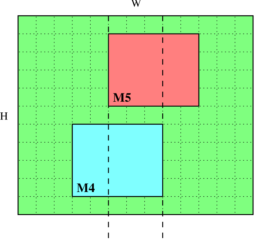
Figure 2: An FPGA of width $W=13$ and height $H=11$. Assume that module M4 of width $w_{4}=5$ and height $h_{4}=4$ is located at position $(3,1)$. If module M5 of same width and height is placed at position $(5,6)$ the resulting overlap is $3$ columns as indicated by the dashed lines. Consequently M4 is interrupted for $3c$ time units.

There is some experimental evidence that an online placement strategy should take this interference into account. As we showed in [6], the least interference fit (LIF) online strategy is quite useful in this setting: New modules are placed in consecutive columns that are used by as few other modules as possible. But in the long term LIF faces two problems:

1. Free space fragmentation: Even though the free space available on the FPGA would allow executing a task on a hardware module (resulting in better quality and/or faster execution), the largest free space fragment available may not be able to accomodate the respective module.

2. Interference: Even though respecting the number of interrupted modules, LIF still has to interrupt modules in the long run.

In this paper we propose a strategy that can increase the long-term quality of the LIF strategy. As described above, our scenario gives rise to times where the system is rather busy. On the other hand, there also are times when the system is more or less offline or unused. These are times when the FPGA could be defragmented. By defragmentation we mean removing modules that have a low usage count and then moving all modules so that a maximal number of columns is unused. This increases the effectiveness of online strategies like LIF.

Defragmentation as described in the paragraph above can be regarded as the two-dimensional strip packing problem. In the next section we will take a closer look at this classic NP-complete optimization problem. As it turns out, for currently relevant numbers of modules, optimal placements can still be computed, using a cutting-edge algorithm for higher-dimensional packing.

III Two-Dimensional Strip Packing

Packing rectangles into a container arises in many industries, whenever steel, glass, wood, or textile materials are to be cut, but it also occurs in less obvious contexts, such as machine scheduling or optimizing the layout of advertisements in newspapers. The three-dimensional problem is important for practical applications such as container loading or scheduling with partitionable resources. For many of these problems, objects must be positioned with a fixed orientation; this requirement also arises when configuring modules on a chip area.

Different types of objective functions for multi-dimensional packing problems have been considered. The Strip Packing Problem (SPP) is to minimize the width $W$ of a strip of fixed height $H$ such that all rectangles fit into a rectangle of size $W\times H$. The orthogonal knapsack problem (OKP) requires selecting a most valuable subset $S$ from a given set of rectangles, such that $S$ can be packed into the large rectangle. The orthogonal bin packing problem (OBPP) considers the scenario in which a supply of containers of a given size is given and the objective is to minimize the number of containers that are needed for packing a set of boxes.

Crucial for all those optimization problems is the corresponding decision problem: The Orthogonal Packing Problem (OPP) is to decide whether a given set of rectangles can be placed within a given rectangle of size $W\times H$. As all of the above problems can be generalized to arbitrary dimensions, we denote by SPP-$d$, OKP-$d$, OBPP-$d$, and OPP-$d$ the strip-packing problem, the orthogonal knapsack problem, the orthogonal bin packing problem, and the orthogonal packing problem, respectively, in $d$ dimensions. (E.g., when considering scheduling problems on an FPGA implies considering two space and one time dimension, yielding $d=3$.) Being a generalization of the one-dimensional problem 3-Partition, the OKP-$d$ is NP-complete in the strict sense, and so the corresponding optimization problems are NP-hard [7].

Dealing with an NP-hard problem (often dubbed “intractable”) does not mean that it is impossible to find provably optimal solutions. While the time for this task may be quite long in the worst case, a good understanding of the underlying mathematical structure may allow it to find an optimal solution (and prove its optimality) in reasonable time for a large number of instances. A good example of this type can be found in [8], where the exact solution of a 120-city instance of the Traveling Salesman Problem is described. In the meantime, benchmark instances of size up to 13509 and 15112 cities have been solved to optimality [9], showing that the right mathematical tools and sufficient computing power may combine to explore search spaces of tremendous size. In this sense, “intractable” problems may turn out to be quite tractable.

Higher-dimensional packing problems have been considered by a great number of authors, but only few of them have dealt with the exact solution of general two-dimensional problems. See [10, 11] for an overview. It should be stressed that unlike one-dimensional packing problems, higher-dimensional packing problems allow no straightforward formulation as integer programs: After placing one box in a container, the remaining feasible space will in general not be convex. Moreover, checking whether a given set of boxes fits into a particular container is trivial in one-dimensional space, but NP-hard in higher dimensions.

Nevertheless, attempts have been made to use standard approaches of mathematical programming. Beasley [12] and Hadjiconstantinou and Christofides [13] have used a discretization of the available positions to an underlying grid to get a 0-1 program with a pseudopolynomial number of variables and constraints. Not surprisingly, this approach becomes impractical beyond instances of rather moderate size.

To our knowledge there is only one work that tries to solve SPP to optimality. In [14] the authors derive improved lower and upper bounds for the two-dimensional strip-packing problem. These bounds are based on a continuous relaxation of the one-dimensional contiguous bin-packing problem (1CBP). These bounds are used in a branch-and-bound type algorithm to solve 27 benchmark instances from the literature.

In [10, 11, 15, 16, 17], a different approach to characterizing feasible packings and constructing optimal solutions is described. A graph-theoretic characterization of the relative position of the boxes in a feasible packing (by so-called packing classes) is used, representing $d$-dimensional packings by a $d$-tuple of interval graphs (called component graphs) that satisfy two extra conditions. This factors out a great deal of symmetries between different feasible packings, it allows to make use of a number of elegant graph-theoretic tools, and it reduces the geometric problem to a purely combinatorial one without using brute-force methods like introducing an underlying coordinate grid. Combined with good heuristics for dismissing infeasible sets of boxes [18], a tree search for constructing feasible packings was developed. This exact algorithm has been implemented; it outperforms previous methods by a clear margin. This approach has been extended to strip-packing problems in the presence of order constraints; see [19]. (Note that in that paper, the emphasis is on the mathematical aspects of dealing with order constraints, not on solving pure strip-packing instances efficiently, as is the case in this paper.)

For the benefit of the reader, a concise description of this approach is contained in the following Section IV.

IV Solving Unconstrained Orthogonal Packing Problems

IV-A A General Framework

If we have an efficient method for solving OPPs, we can also solve SPPs by using a binary search. However, deciding the existence of a feasible packing is a hard problem in higher dimensions, and proposed methods suggested by other authors [12, 13] have been of limited success.

Our framework uses a combination of different approaches to overcome these problems, see Figure 3:

1. Try to disprove the existence of a packing by classes of lower bounds on the necessary size.

2. In case of failure, try to find a feasible packing by using fast heuristics.

3. If the existence of a packing is still unsettled, start an enumeration scheme in form of a branch-and-bound tree search.

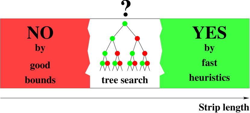
Figure 3: The basic idea of our binary search.

By developing good new bounds for the first stage, we have been able to achieve a considerable reduction of the number of cases where a tree search needs to be performed. (Mathematical details for this step are described in [18, 15].) However, it is clear that the efficiency of the third stage is crucial for the overall running time when considering difficult problems. Using a purely geometric enumeration scheme for this step by trying to build a partial arrangement of boxes is easily seen to be immensely time-consuming. In the following, we describe a purely combinatorial characterization of feasible packings that allows to perform this step more efficiently.

IV-B Packing Classes

Consider a feasible packing in $d$-dimensional space, and project the boxes onto the $d$ coordinate axes. This converts the one $d$-dimensional arrangement into $d$ one-dimensional ones (see Figure 4 for an example in $d=2$). By disregarding the exact coordinates of the resulting intervals in direction $i$ and only considering their intersection properties, we get the component graph $G_{i}=(V,E_{i})$: Two boxes $u$ and $v$ are connected by an edge in $G_{i}$, iff their projected intervals in direction $x_{i}$ have a non-empty intersection. By definition, these graphs are interval graphs. This class of graphs has been studied intensively in graph theory (see [20, 21]), and it has a number of very useful algorithmic properties.

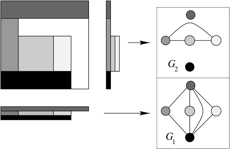
Figure 4: The projections of the boxes onto the coordinate axes define interval graphs (here in 2D: $G_{1}$ and $G_{2}$).

Considering sets of $d$ component graphs $G_{i}$ instead of complicated geometric arrangements has some clear advantages (algorithmic implications for our specific purposes are discussed further down). It is not hard to check that the following three conditions must be satisfied by all $d$-tuples of graphs $G_{i}$ that are constructed from a feasible packing:

1. $G_{i}$ is an interval graph, $\forall i\in\{1,\cdots,d\}$.

2. Any independent set $S$ of $G_{i}$ is $i$-admissible, $\forall i\in\{1,\cdots,d\}$, i.e., $w_{i}(S)=\sum_{v\in S}w_{i}(v)\leq h_{i}$, because all boxes in $S$ must fit into the container in the $i$th dimension.

3. $\cap_{i=1}^{d}E_{i}=\emptyset$. In other words, there must be at least one dimension in which the corresponding boxes do not overlap.

A $d$-tuple of component graphs satisfying these necessary conditions is called a packing class. The remarkable property (proven in [22, 11]) is that these three conditions are also sufficient for the existence of a feasible packing.

Theorem IV.1 (Fekete, Schepers)

A set of boxes allows a feasible packing, iff there is a a packing class, i. e., a $d$-tuple of graphs $G_{i}=(V,E_{i})$ that satisfies the conditions C1, C2, C3.

This allows it to consider only packing classes in order to decide the existence of a feasible packing, and to disregard most of the geometric information. See Figure 5 to see how a packing class gives rise to a feasible packing; note that this packing is not identical to the one in Figure 4. (In fact, there are many possible packings for a packing class, see the following subsection and Figure 5.)

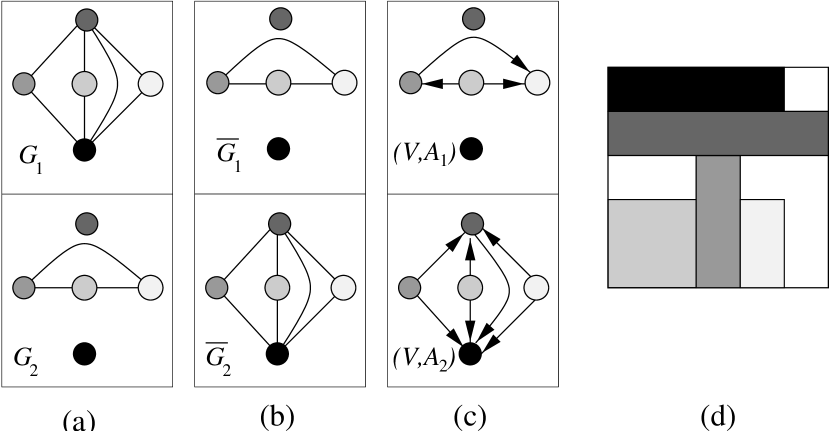
Figure 5: (a) A two-dimensional packing class. (b) The corresponding comparability graphs. (c) The transitive orientations. (d) A feasible packing corresponding to the orientation.

IV-C Solving OPPs

Our search procedure works on packing classes, i.e., $d$-tuples of component graphs with the properties C1, C2, C3. Because each packing class represents not only a single packing but a whole family of equivalent packings, we are effectively dealing with more than one possible candidate for an optimal packing at a time. (The reader may check for the example in Figure 4 that there are 36 different feasible packings that correspond to the same packing class.)

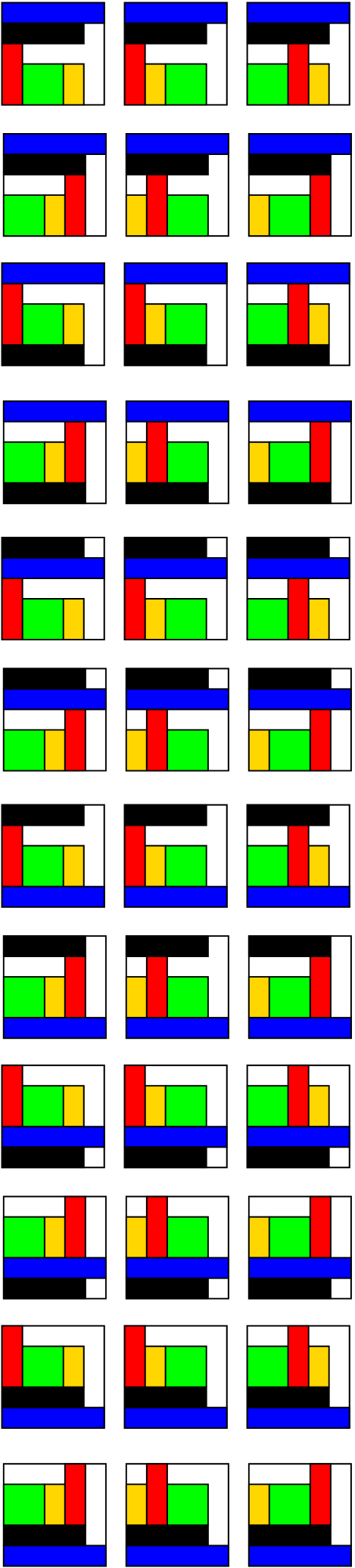
Figure 6: All shown 36 packings correspond to the component graphs $G_{1}$ and $G_{2}$ that are shown in Figure 4.

For finding an optimal packing, we use a branch-and-bound approach. The search tree is traversed by depth first search, see [16, 22] for details. Branching is done by fixing an edge $\{b,c\}\in E_{i}$ or $\{b,c\}\notin E_{i}$. After each branching step, it is checked whether one of the three conditions C1, C2, C3 is violated; furthermore it is checked, whether a violation can only be avoided by fixing further edges. Testing for two of the conditions C1–C3 is easy: enforcing C3 is obvious; property C2 is hereditary, so adding edges to $E_{i}$ later will keep it satisfied. (Note that computing maximum weighted cliques on comparability graphs can be done efficiently, see [20].) In order to ensure that property C1 is not violated, we use some graph-theoretic characterizations of interval graphs and comparability graphs. These characterizations are based on two forbidden substructures (again, see [20] for details; the first condition is based on the classical characterizations by [23, 24]: a graph is an interval graph iff its complement has a transitive orientation, and it does not contain any induced chordless cycle of length 4.) In particular, the following configurations have to be avoided:

1. induced chordless cycles of length 4 in $E_{i}$;

2. so-called 2-chordless odd cycles in the set $\overline{E_{i}}$ of edges excluded from $E_{i}$ (see [16, 20] for details);

3. infeasible stable sets in $E_{i}$.

Each time we detect such a fixed subgraph, we can abandon the search on this node. Furthermore, if we detect a fixed subgraph, except for one unfixed edge, we can fix this edge, such that the forbidden subgraph is avoided.

Our experience shows that in the considered examples these conditions are already useful when only small subsets of edges have been fixed, because by excluding small sub-configurations, like induced chordless cycles of length 4, each branching step triggers a cascade of more fixed edges.

V Computational Results

• $\textnormal{DefragmentModuleLayout}()$
     1$LB\leftarrow\textnormal{CalculateLowerBound()}$ 2$UB\leftarrow\textnormal{CalculateUpperBound()}$ 3while $LB\neq UB$ do 4 $W\leftarrow LB+\left\lfloor\frac{LB+UB}{2}\right\rfloor$ 5 if SolveOPP(W) then 6 $LB\leftarrow W$ 7 else 8 $UB\leftarrow W$

Figure 7: The binary search algorithm for determining an optimal module layout. In this algorithm the OPP as described in section IV is solved repeatedly to determine if all modules fit in a strip of width $W$. This search is iterated until an optimal solution is found.

We have used our implementation for the OPP (as described in the previous section) as a building block for our new strip-packing code. To allow for a later implementation of the strip-packing code on the MicroBlaze cores we have used very simple lower and upper bounds to restrict the binary search interval: Let $I$ denote the indices of the modules present on the FPGA. Then the lower bound for the number of columns $W_{L}$ we used is given by

$$W_{L}=\left\lceil\frac{\sum_{i\in I}w_{i}h_{i}}{H}\right\rceil.$$

The upper bound is computed as the minimum of the three shelf-packing heuristics next-fit-decreasing, first-fit-decreasing and best-fit-decreasing [25]. These heuristics partition the strip into shelves. A new shelf of height $h_{j}$ is created if there is no shelf in which the module $j$ can be placed. If the module can be placed in more than one shelf the shelf is picked according to the next-fit, first-fit, or best-fit strategy respectively.

Based on these bounds the algorithm performs a binary search until an optimal soution is found. The algorithm is outlined in Figure 7.

We have benchmarked our code against a set of 10 instances. Considering our multimedia scenario, we have constrained different IP cores like MPEG2 decoders, MP3 decoders, MicroBlaze core, interface modules like CAN, CardBus, etc. to rectangular shape. We consider one busy time, where many modules are placed and removed from the FPGA. The placement strategy we used was LIF. For the removal of the FPGAs we used the least-recently-used (LRU) strategy. The result is shown in Figure 8. This is followed by the removal of some randomly selected modules. For these instances we report the maximal free rectangle and the number of free columns before and after defragmentation. On an Intel Pentium IV clocked at 3GHz the running time was less than 0.5 s for each scenario.

As shown in Table I defragmentation increases the area of the maximal free rectangle and the number of free columns in all of the 10 scenarios. The smallest increase in area can be seen in scenarios E and J. Here a factor of 1.4 is obtained. In scenarios A and C an increase of area of the maximal rectangle reaches its maximum with a factor of 3.1. On average, the area of the maximal free rectangle is increased by a factor of 2.2. The number of free columns grows at least two and by at most six. The average increase of free columns is 4.2.

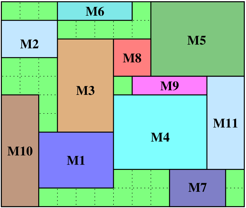
Figure 8: The FPGA before defragmentation. Even though the remaining free space is 30 reconfigurable units (RFUs), the maximal free rectangle of dimension $7\times 1$ has only 7 RFUs. Note that there is no free column.

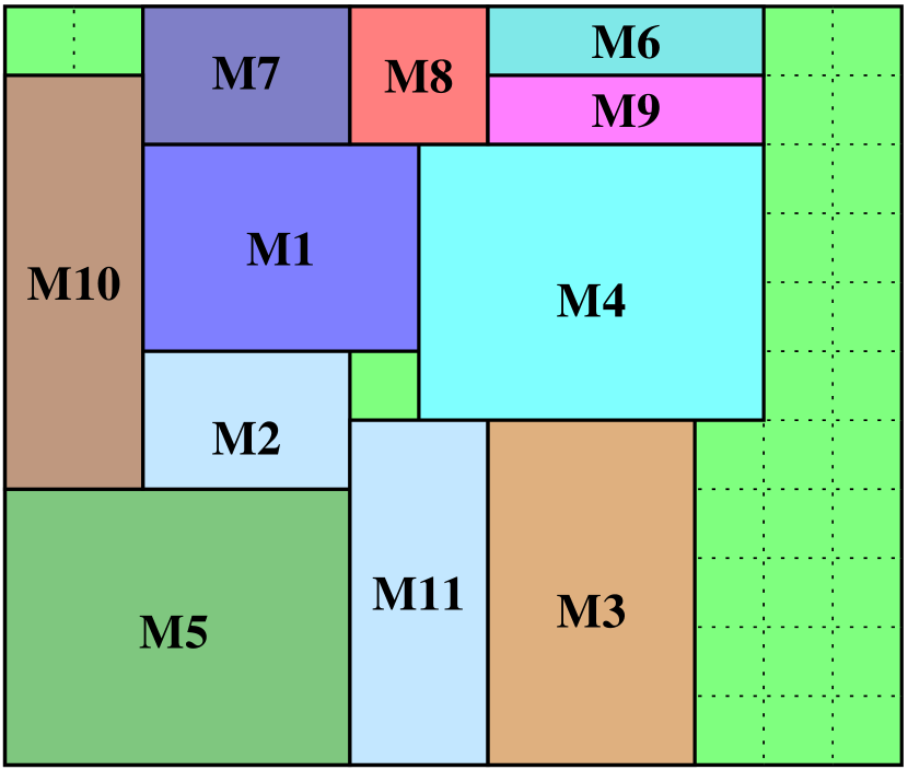
Figure 9: The same FPGA as in Figure 8 after defragmentation. The remaining free space is 30 reconfigurable units (RFUs). Now the maximal free rectangle is of dimension $2\times 11$ has 22 RFUs. The number of free columns is 2.

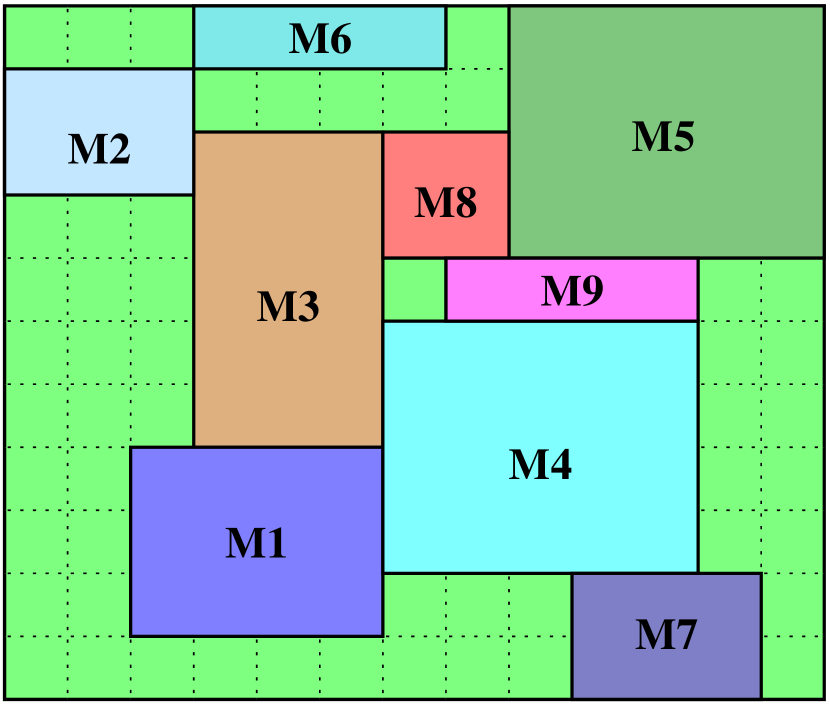
Figure 10: The same FPGA as in Figure 8. Modules M10 and M11 have been removed due to a low usage count. The remaining free space is now 52 RFUs. The largest free rectangle has dimension $2\times 8$ and 16 RFUs. There still is no free column.

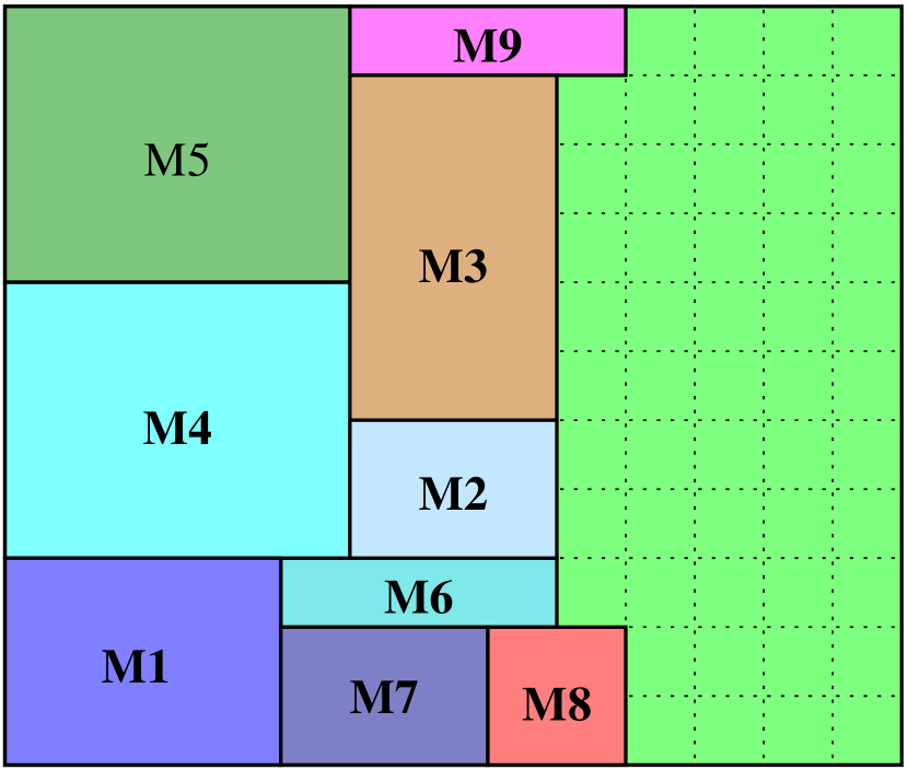
Figure 11: The same FPGA as in Figure 9 after succesful defragmentation. The free space of 52 RFUs is the same as before. The largest free rectangle has grown to dimension $4\times 11$ and contains 44 RFUs. Now there are 4 free columns.

			Before defragmentation		After defragmentation
Scenario	$|I|$	Free space	Max. rectangle	Free columns	Max. rectangle	Free columns
A	11	30	$7\times 1$	0	$2\times 11$	2
B	9	52	$2\times 8$	0	$4\times 11$	4
C	9	70	$3\times 7$	0	$6\times 11$	6
D	9	42	$4\times 4$	0	$3\times 11$	3
E	6	83	$6\times 8$	0	$6\times 11$	6
F	6	54	$8\times 2$	0	$4\times 11$	4
G	5	76	$6\times 4$	2	$6\times 11$	6
H	6	53	$3\times 11$	3	$4\times 11$	7
I	5	87	$9\times 6$	1	$7\times 11$	7
J	6	42	$3\times 8$	0	$3\times 11$	3

TABLE I: Results for ten different scenarios, based on Figure 8. The solution for scenario A is shown in Figure 9, the others have modules removed from the FPGA. Scenario B is shown in Figure 10, its solution in Figure 11. The next columns show the number of placed modules, the total free space, the maximal free rectangle, and the number of free columns before defragmentation. The final columns show results after defragmentation.

VI Conclusions

We have shown that mixing online and offline strategies can improve the overall reconfiguration process in partial reconfiguration. Especially for FPGAs with partial reconfiguration restricted to columnwise reconfiguration, a defragmentation strategy as proposed in this paper helps to reduce the interference with other modules.

There are many possible extensions to our approach. We list two of them explicitly:

1. Malleable modules: Tools for automatic synthesis normally do not create modules with rectangular shape. Instead, width and height of the modules can be chosen freely within certain technical bounds. This gives more room for the optimization in the defragmentation process. In a mathematical context this model would be called a class strip packing problem: Given a set of modules that has to be placed on a chip as to minimize the total number of columns used, choose for each module from a certain set of module realizations and try to find a placement.

   If the width and height of the modules can be chosen freely this problem is known as strip packing with modifiable boxes. In an offline setting this problem can be trivially solved by applying once the volume lower bound as described above and then setting the height of each box to this value. In [26] the author gives a 4-competitive online algorithm for the problem and shows that no online algorithm can do better than 1.73.

2. Fixed modules: In most FPGA designs, pins of the FPGA are hard-wired. In this setting it may be unavoidable to fix a placement of the respective interface modules in close proximity to their IO pins. When this is the case, the defragmentation problem is no longer a strip-packing problem. Freeing as many columns as possible can be achieved by placing other modules above or below the interface modules and not just as far as possible to the left.

We are optimistic that our general approach will allow some progress on these problem classes.

References

- [1] C. Steiger, H. Walder, and M. Platzner, “Operating systems for reconfigurable embedded platforms: Online scheduling of real-time tasks,” IEEE Transaction on Computers, vol. 53, no. 11, pp. 1393–1407, 2004.
- [2] O. Diessel, H. ElGindy, M. Middendorf, H. Schmeck, and B. Schmidt, “Dynamic scheduling of tasks on partially reconfigurable FPGAs,” IEE Proceedings – Computers and Digital Techniques, vol. 147, no. 3, pp. 181–188, May 2000.
- [3] Virtex-II platform FPGAs: Complete data sheet, XILINX Inc., June 2004.
- [4] C. Bobda, M. Majer, D. Koch, A. Ahmadinia, and J. Teich, “A dynamic NoC approach for communication in reconfigurable devices,” in Proceedings of International Conference on Field-Programmable Logic and Applications (FPL), ser. Lecture Notes in Computer Science (LNCS), vol. 3203. Antwerp, Belgium: Springer, Aug. 2004, pp. 1032–1036.
- [5] E. L. Lawler, J. K. Lenstra, A. H. G. Rinooy Kan, and D. B. Shmoys, “Sequencing and scheduling: Algorithms and complexity,” in Logistics of Production and Inventory, ser. Handbooks in Operations Research and Management, vol. 4, S. C. Graves, A. H. G. Rinnooy Kan, and P. H. Zipkin, Eds. North–Holland, Amsterdam, 1993, pp. 445–522.
- [6] A. Ahmadinia and J. Teich, “Speeding up online placement for XILINX FPGAs by reducing configuration overhead,” in Proceedings of the IFIP International Conference on VLSI-SOC. Darmstadt, Germany: IFIP, Dec. 2003, pp. 118–122.
- [7] M. R. Garey and D. S. Johnson, Computers and Intractability: A Guide to the Theory of NP-Completeness. New York: Freeman, 1979.
- [8] M. Grötschel, “On the symmetric travelling salesman problem: solution of a 120-city problem,” Mathematical Programming Study, vol. 12, pp. 61–77, 1980.
- [9] D. Applegate, R. Bixby, V. Chvátal, and W. Cook, “On the solution of traveling salesman problems,” Documenta Mathematica Journal der Deutschen Mathematiker-Vereinigung, vol. ICM III, pp. 645–656, 1998.
- [10] S. P. Fekete and J. Schepers, “A new exact algorithm for general orthogonal d-dimensional knapsack problems,” in Algorithms – ESA ’97, vol. 1284, Springer Lecture Notes in Computer Science, 1997, pp. 144–156.
- [11] ——, “A combinatorial characterization of higher-dimensional orthogonal packing,” Mathematics of Operations Research, vol. 29, pp. 353–368, 2004.
- [12] J. E. Beasley, “An exact two-dimensional non-guillotine cutting tree search procedure,” Operations Research, vol. 33, pp. 49–64, 1985.
- [13] E. Hadjiconstantinou and N. Christofides, “An exact algorithm for general, orthogonal, two-dimensional knapsack problems,” European Journal of Operations Research, vol. 83, pp. 39–56, 1995.
- [14] S. Martello, M. Monaci, and D. Vigo, “An exact approach to the strip-packing problem,” INFORMS Journal on Computing, vol. 15, no. 3, pp. 310–319, 2003.
- [15] S. P. Fekete and J. Schepers, “A general framework for bounds for higher-dimensional orthogonal packing problems,” Mathematical Methods of Operations Research, vol. 60, pp. 311–329, 2004.
- [16] ——, “An exact algorithm for higher-dimensional packing,” Operations Research, to appear.
- [17] J. Teich, S. P. Fekete, and J. Schepers, “Optimal hardware reconfiguration techniques,” Journal of Supercomputing, vol. 19, pp. 57–75, 2001.
- [18] S. P. Fekete and J. Schepers, “New classes of lower bounds for bin packing problems,” in Integer Programming and Combinatorial Optimization (IPCO’98), ser. Springer Lecture Notes in Computer Science, vol. 1412, 1998, pp. 257–270.
- [19] S. P. Fekete, E. Köhler, and J. Teich, “Multi-dimensional packing with order constraints,” in Proceedings 7th International Workshop on Algorithms and Data Structures, ser. Lecture Notes in Computer Science, vol. 2125. Springer-Verlag, 2001, pp. 300–312.
- [20] M. C. Golumbic, Algorithmic graph theory and perfect graphs. New York: Academic Press, 1980.
- [21] R. H. Möhring, “Algorithmic aspects of comparability graphs and interval graphs,” in Graphs and Order, I. Rival, Ed. D. Reidel Publishing Company, Dordrecht, 1985, pp. 41–101.
- [22] J. Schepers, “Exakte Algorithmen für orthogonale Packungsprobleme,” Universität Köln, Tech. Rep. 97-302, Doctoral thesis, 1997.
- [23] A. Ghouilà-Houri, “Caractérization des graphes non orientés dont on peut orienter les arrêtes de manière à obtenir le graphe d’une relation d’ordre,” C.R. Acad. Sci. Paris, vol. 254, pp. 1370–1371, 1962.
- [24] P. C. Gilmore and A. J. Hoffmann, “A characterization of comparability graphs and of interval graphs,” Canadian Journal of Mathematics, vol. 16, pp. 539–548, 1964.
- [25] B. S. Baker and J. S. Schwarz, “Shelf algorithms for two-dimensional packing problems,” SIAM Journal on Computing, vol. 12, no. 3, pp. 508–525, 1983.
- [26] C. Imreh, “Online strip packing with modifiable boxes,” Operations Research Letters, vol. 29, no. 2, pp. 79–85, 2001.