Abstract

Ever since entanglement was identified as a computational and cryptographic resource, effort has been made to find an efficient way to tell whether a given density matrix represents an unentangled, or separable, state. Essentially, this is the quantum separability problem.

In Chapter 1, I begin with a brief introduction to quantum states, entanglement, and a basic formal definition of the quantum separability problem. I conclude the first chapter with a summary of one-sided tests for separability, including those involving semidefinite programming.

In Chapter 2, I apply polyhedral theory to prove easily that the set of separable states is not a polytope; for the sake of completeness, I then review the role of polytopes in nonlocality. Next, I give a novel treatment of entanglement witnesses and define a new class of entanglement witnesses, which may prove to be useful beyond the examples given. In the last section, I briefly review the five basic convex body problems given in [1], and their application to the quantum separability problem.

In Chapter 3, I treat the separability problem as a computational decision problem and motivate its approximate formulations. After a review of basic complexity-theoretic notions, I discuss the computational complexity of the separability problem: I discuss the issue of NP-completeness, giving an alternative definition of the separability problem as an NP-hard problem in NP. I finish the chapter with a comprehensive survey of deterministic algorithmic solutions to the separability problem, including one that follows from a second NP formulation.

Chapters 1 to 3 motivate a new interior-point algorithm which, given the expected values of a subset of an orthogonal basis of observables of an otherwise unknown quantum state, searches for an entanglement witness in the span of the subset of observables. When all the expected values are known, the algorithm solves the separability problem. In Chapter 4, I give the motivation for the algorithm and show how it can be used in a particular physical scenario to detect entanglement (or decide separability) of an unknown quantum state using as few quantum resources as possible. I then explain the intuitive idea behind the algorithm and relate it to the standard algorithms of its kind. I end the chapter with a comparison of the complexities of the algorithms surveyed in Chapter 3. Finally, in Chapter 5, I present the details of the algorithm and discuss its performance relative to standard methods.

Preface

This work attempts to give a comprehensive treatment of the state of the art in deterministic algorithms for the quantum separability problem in the finite-dimensional and bipartite case. The need for such a treatment stems from the very recent (2003 and later) proposals for separability algorithms – all quite different from one another. It is likely that these recent papers emerged when they did because of the (disheartening) result of Gurvits (2001) showing the problem to be computationally intractable: given that the problem is hard, what is the best we can do to solve it? Among these proposals is my algorithm (done in collaboration), which will be shown to compare favorably to the others, complexity-theoretically.

Gurvits’ result, that the separability problem is NP-hard, raised a question among the quantum information community: “…but then isn’t it NP-complete?” After hearing many people ask this question, I set out to clarify the issue and show that the separability problem is NP-complete in the usual sense (that is, with respect to Karp reductions). The latter part of this mission is as yet unsuccessful, but the partial results are presented, including a redefining of the separability problem as an NP-hard problem in NP (previous definitions could not place the problem in NP, rather only in a modified version of NP).

Entanglement witnesses have been around since 1996, and had been extensively studied up until recently, especially by the Innsbruck-Hannover group, which produced interesting characterisations of entanglement witnesses and showed how to construct optimal entanglement witnesses. I approached entanglement witnesses from the viewpoint of polyhedral theory, rather than linear-operator theory. The result was the immediate solution of an open problem of whether the separable states form a polytope. Under a slightly different definition of “entanglement witness”, I discover a new class of entanglement witnesses which I call “ambidextrous entanglement witnesses”. These correspond to observables whose expected values can indicate that a state is entangled on opposite sides of the set of separable states.

Acknowledgements

I am utterly grateful to my supervisor, Artur Ekert, for his support and encouragement; his liberal approach to supervision, which allowed me to pursue my own interests; and for his prophetic suggestion of my thesis title on the day I arrived in Cambridge.

I am also grateful to the GCHQ for funding this PhD. Much travel was also funded by project RESQ (IST-2001-37559) of the IST-FET programme of the EC.

The main result in this thesis came out of my collaboration with my main co-authors, Ben Travaglione and Donny Cheung. I would especially like to thank Ben for essentially co-supervising me during the first two years of my degree. Discussions with Daniel Gottesman formed the basis of the NP-formulation of the quantum separability problem.

Tom Stace has been extremely generous with his time, always willing to engage in a discussion about the various elements of my work around which I was having trouble wrapping my head. He was very helpful during early stages of the development of the algorithm.

Coralia Cartis introduced me to logarithmic barriers, analytic centres, and self-concordance; and confirmed my intuition that the analytic centre in Chapter 5 was indeed a conic combination of the normal vectors, where I was too inept to calculate $\nabla F$ correctly the first time around.

Matthias Christandl taught me about entanglement measures and pointed me to the work of König and Renner on the finite quantum de Finetti theorem. Other colleagues who have been helpful are Carolina Moura Alves, Garry Bowen, and Daniel Oi.

My examiners made many comments and suggestions which greatly improved this thesis.

My parents, Art and Josie Ioannou, and brother, John Ioannou, have been incredibly loving and supportive throughout my studies.

It was absolutely wonderful to marry Sarah Tait in 2005! She has been a pillar of support. She took a risk in coming to Cambridge with me; I am happy that she is happy here. I love her.

List of Publications

The following is a list of papers that have resulted from the work presented in this thesis.

1. L. M. Ioannou and B. C. Travaglione, A note on quantum separability, quant-ph/0311184.

2. L. M. Ioannou, B. C. Travaglione, D. Cheung, A. K. Ekert, Improved algorithm for quantum separability and entanglement detection, Physical Review A, 70 060303(R) (2004).

3. L. M. Ioannou, B. C. Travaglione, D. Cheung, Separation from optimization using analytic centers, cs.DS/0504110.

4. L. M. Ioannou and B. C. Travaglione, Quantum separability and entanglement detection via entanglement-witness search (in preparation).

List of Figures

1. 3.1 Surface on boundary of $\mathcal{S}_{M,N}$
2. 4.1 The sets $M_{p}$ and $K_{p}$ in $\mathbb{R}^{2}$
3. 4.2 Illustration of intuitive heuristic behind Lemma 14
4. 4.3 Relationship between convex separation methods
5. 5.1 The solid angle $\theta_{1}+\theta_{2}$ of the hypercircular-based cone
6. 5.2 Derivation of solid angle $2\theta$ of hypercircular-based cone in terms of $R$ and $\delta$.
7. 5.3 Derivation of radius $r$ as a function of $\theta$.
8. 5.4 Schematic diagram of density operators

Contents

1. Abstract
2. Preface
   1. Acknowledgements
3. 1 Introduction
   1. 1.1 Quantum physics
   2. 1.2 One-sided tests and restrictions
   3. 1.3 One-sided tests based on semidefinite programming
      1. 1.3.1 A test based on symmetric extensions
      2. 1.3.2 A test based on semidefinite relaxations
      3. 1.3.3 Entanglement Measures
      4. 1.3.4 Other tests
4. 2 Convexity
   1. 2.1 Polyhedra and $\mathcal{S}_{M,N}$
   2. 2.2 Entanglement witnesses
      1. 2.2.1 Experimental separability
      2. 2.2.2 Polytopes in separability and nonlocality
      3. 2.2.3 Ambidextrous entanglement witnesses
   3. 2.3 Convex body problems
5. 3 Separability as a Computable Decision Problem
   1. 3.1 Formulating the quantum separability problem
      1. 3.1.1 Exact formulations
      2. 3.1.2 Approximate formulations
   2. 3.2 Computational complexity
      1. 3.2.1 Review of NP-completeness
      2. 3.2.2 Quantum separability problem in NP
      3. 3.2.3 NP-Hardness
      4. 3.2.4 Towards a Karp Reduction
      5. 3.2.5 Nonmembership in co-NP
   3. 3.3 Survey of algorithms for the quantum separability problem
      1. 3.3.1 Search for separable decompositions
      2. 3.3.2 Bounded search for symmetric extensions
      3. 3.3.3 Cross-norm criterion via linear programming
      4. 3.3.4 Fixed-point iterative method
6. 4 Reduction to Entanglement Witness Search
   1. 4.1 Overview
   2. 4.2 Reduction to optimisation
   3. 4.3 Detecting Entanglement of an Unknown State Using Partial Information
   4. 4.4 New method to solve separation with optimisation
   5. 4.5 Connection to standard method
   6. 4.6 Cutting-plane algorithms for convex feasibility for $K^{\prime}$
   7. 4.7 A new quantum separability algorithm
   8. 4.8 Complexity comparison of algorithms
7. 5 New polynomial-time reduction from WSEP to WOPT
   1. 5.1 The Main Idea of the Algorithm
   2. 5.2 The Algorithm
   3. 5.3 Proof of Correctness of the Algorithm
      1. 5.3.1 Convergence
      2. 5.3.2 Producing Good Cutting Planes
      3. 5.3.3 Derivation of $r$
      4. 5.3.4 Newton Iterates
      5. 5.3.5 Selecting the Constants
      6. 5.3.6 Tighter Stopping Conditions
   4. 5.4 Complexity and Discussion
   5. 5.5 Application to Quantum Separability Problem
   6. 5.6 Closing remarks
8. A Convergence proofs

Chapter 1 Introduction

“Just because it’s hard, it doesn’t mean you don’t try.” When my mother said these words to me way back when I was a Master’s student, I had no idea they would open my PhD thesis.

Ever since quantum-mechanical phenomena were identified as computational and cryptographic resources, researchers have become even more interested in precisely characterising the features of quantum theory that set it apart from classical physical theory. Two of these features are nonlocality and entanglement, both of which are “provably hard” to characterise; that is, deciding whether a quantum state exhibits nonlocality or entanglement is as hard as some of the hardest and most important problems in complexity theory.

This thesis concentrates on the latter problem of deciding whether a quantum state is unentangled, or, separable. I review all of the deterministic algorithms proposed for the separability problem, including two of my own, in an attempt to discover which has the best asymptotic complexity. Along the way, I look at entanglement witnesses in a new light and discuss the computational complexity of the separability problem.

In Section 1.1, I review some elements of quantum mechanics and define and give the significance of separable states. The remainder of the chapter discusses partial solutions to the separability problem.

1.1 Quantum physics

The pure state of a $d$-dimensional quantum physical system is represented mathematically by a complex unit-vector $\left|\psi\right>\in\mathbb{C}^{d}$, where the “global phase” of $\left|\psi\right>$ is irrelevant; that is, for any real $\phi$, $e^{i\phi}\left|\psi\right>$ represents the same physical state as $\left|\psi\right>$. If the system can be physically partitioned into two subsystems (denoted by superscripts $\mathrm{A}$ and $\mathrm{B}$) of dimensions $M$ and $N$, such that $d=MN$, then $\left|\psi\right>$ may be separable, which means $\left|\psi\right>=\left|\psi^{\mathrm{A}}\right>\otimes\left|\psi^{\mathrm{B}}\right>$, for $\left|\psi^{\mathrm{A}}\right>\in\mathbf{C}^{M}$ and $\left|\psi^{\mathrm{B}}\right>\in\mathbf{C}^{N}$ and where “$\otimes$” denotes the Kronecker (tensor) product. Without loss of generality, assume $M\leq N$ unless otherwise stated. If $\left|\psi\right>$ is not separable, then it is entangled (with respect to that particular partition).

More generally, the state of the system may be a mixed state, which is a statistical distribution of pure states. A mixed state $\rho$ is usually represented as the density operator $\rho=\sum_{i=1}^{k}p_{i}\left|\psi_{i}\right>\left<\psi_{i}\right|$, where $\left|\psi_{i}\right>\in\mathbf{C}^{d}$, $\sum_{i=1}^{k}p_{i}=1$, $p_{i}\geq 0$, and $\left<\psi_{i}\right|$ is the dual vector of $\left|\psi_{i}\right>$. A mixed state is thus a positive semidefinite (and hence Hermitian, or self-adjoint) operator with unit trace: $\rho\geq 0$ and $\textrm{tr}(\rho)=1$. Denote the set of all density operators mapping complex vector space $V$ to itself by $\mathcal{D}(V)$; let $\mathcal{D}_{M,N}:=\mathcal{D}(\mathbb{C}^{M}\otimes\mathbb{C}^{N})$. The maximally mixed state is $I_{M,N}:=I/MN$, where $I$ denotes the identity operator. A density operator $\rho$ satisfies $0\leq\textrm{tr}(\rho^{2})\leq 1$ and represents a pure state if and only if $\textrm{tr}(\rho^{2})=1$. A pure state $\left|\psi\right>$ is separable if and only if $\textrm{tr}_{\mathrm{B}}(|\psi\rangle\langle\psi|)$ is a pure state, where “$\textrm{tr}_{\mathrm{B}}$” denotes the partial trace with respect to subsystem $\mathrm{B}$ (e.g. see Exercise 2.78 in [2]); a pure state is called maximally entangled if $\textrm{tr}_{\mathrm{B}}(|\psi\rangle\langle\psi|)$ is the maximally mixed state $I/M$ in the space of density operators on the $\mathrm{A}$-subsystem $\mathcal{D}(\mathbb{C}^{M})$. Thus, the mixedness of $\textrm{tr}_{\mathrm{B}}(|\psi\rangle\langle\psi|)$ is some “measure” of the entanglement of $\left|\psi\right>$ (see Section 1.3.3).

A mixed state $\rho\in\mathcal{D}_{M,N}$ is separable if and only if it may be written $\rho=\sum_{i=1}^{k}p_{i}\rho^{\mathrm{A}}_{i}\otimes\rho^{\mathrm{B}}_{i}$ with $p_{i}\geq 0$ and $\sum_{i}p_{i}=1$, and where $\rho^{\mathrm{A}}_{i}\in\mathcal{D}(\mathbb{C}^{M})$ is a (mixed or pure) state of the $A$-subsystem (and similarly for $\rho^{\mathrm{B}}_{i}\in\mathcal{D}(\mathbb{C}^{N})$); when $k=1$, $\rho$ is a product state. Let $\mathcal{S}_{M,N}\subset\mathcal{D}_{M,N}$ denote the separable states; let $\mathcal{E}_{M,N}:=\mathcal{D}_{M,N}\setminus\mathcal{S}_{M,N}$ denote the entangled states. The following fact will be used several times throughout this thesis:

Fact 1 ([3]).

If $\sigma\in\mathcal{S}_{M,N}$, then $\sigma$ may be written as a convex combination of $M^{2}N^{2}$ pure product states, that is,

$$\sigma=\sum_{i=1}^{M^{2}N^{2}}p_{i}|\psi^{\mathrm{A}}_{i}\rangle\langle\psi^{\mathrm{A}}_{i}|\otimes|\psi^{\mathrm{B}}_{i}\rangle\langle\psi^{\mathrm{B}}_{i}|,$$ (1.1)

where $\sum_{i=1}^{M^{2}N^{2}}p_{i}=1$ and $0\leq p_{i}\leq 1$ for all $i=1,2,\ldots,M^{2}N^{2}$.

Recall that a set of points $\{x_{1},\ldots,x_{j}\}\subset\mathbb{R}^{n}$ is affinely independent if and only if the set $\{x_{2}-x_{1},x_{3}-x_{1},\ldots,x_{j}-x_{1}\}$ is linearly independent in $\mathbb{R}^{n}$. Recall also that the dimension of $X\subset\mathbb{R}^{n}$ is defined as the size of the largest affinely-independent subset of $X$ minus 1. Fact 1 is based on the well-known theorem of Carathéodory that any point in a compact convex set $X\subset\mathbb{R}^{n}$ of dimension $k$ can be written as a convex combination of $k+1$ affinely-independent extreme points of $X$.

Definition 1 (Formal quantum separability problem).

Let $\rho\in\mathcal{D}_{M,N}$ be a mixed state. Given the matrix $[\rho]$ (with respect to the standard basis of $\mathbb{C}^{M}\otimes\mathbb{C}^{N}$) representing $\rho$, decide whether $\rho$ is separable.

What is the significance of a separable state? For a pure state $\left|\psi\right>=\left|\psi^{\mathrm{A}}\right>\otimes\left|\psi^{\mathrm{B}}\right>$, we can imagine two spatially separated people (laboratories) – called “Alice” (“A”) and “Bob” (“B”) – who each have one part of $\left|\psi\right>$: Alice has $\left|\psi^{\mathrm{A}}\right>$ and Bob has $\left|\psi^{\mathrm{B}}\right>$. We can further imagine that Alice and Bob each prepared their respective part of the state $\left|\psi\right>$; i.e. Alice prepared a pure state $\left|\psi^{\mathrm{A}}\right>$ and Bob prepared a pure state $\left|\psi^{\mathrm{B}}\right>$, and $\left|\psi\right>$ describes the state of the union of Alice’s system and Bob’s system.

In preparing their systems, Alice and Bob could use classical randomness. Thus, instead of preparing the pure state $\left|\psi^{\mathrm{A}}\right>$ with probability 1, Alice prepares the state $\left|\psi^{\mathrm{A}}_{i}\right>$ with probability $p^{\mathrm{A}}_{i}$. By imagining infinitely many repeated trials of this whole scenario, this means Alice prepares the mixed state $\rho^{\mathrm{A}}=\sum_{i}p^{\mathrm{A}}_{i}|\psi^{\mathrm{A}}_{i}\rangle\langle\psi^{\mathrm{A}}_{i}|$. Similarly, Bob could prepare his subsystem in the mixed state $\rho^{\mathrm{B}}$. The state of the total system is then represented by $\rho^{\mathrm{A}}\otimes\rho^{\mathrm{B}}$. States of this form can thus be prepared with local (randomised) operations.

Now suppose that Alice and Bob can telephone each other. Then they could coordinate their subsystem-preparations: when Alice (through her local randomness) decides (with probability $p_{i}$) to prepare $\left|\psi^{\mathrm{A}}_{i}\right>$, she tells Bob to prepare $\left|\psi^{\mathrm{B}}_{i}\right>$. The state of the total system is now represented by

$$\rho=\sum_{i}p_{i}|\psi^{\mathrm{A}}_{i}\rangle\langle\psi^{\mathrm{A}}_{i}|\otimes|\psi^{\mathrm{B}}_{i}\rangle\langle\psi^{\mathrm{B}}_{i}|,$$ (1.2)

which may not have a representation of the form $\rho^{\mathrm{A}}\otimes\rho^{\mathrm{B}}$. States of the form (1.2) can thus be prepared with local operations and classical communication (abbreviated “LOCC”). These are the separable states. Instead of a telephone (two-way classical channel), it suffices that Alice and Bob share a source of randomness in order to create a separable state.

If Alice and Bob share an entangled state (perhaps Alice prepared the total system and then sent the B-subsystem to Bob), then they share something that they could not have made with LOCC. Perhaps unsurprisingly, it turns out that sharing certain types of entangled states (see Section 2.2.2) allows Alice and Bob to communicate in ways that they could not have with just a telephone [4, 2].

1.2 One-sided tests and restrictions

Shortly after the importance of the quantum separability problem was recognised in the quantum information community, efforts were made to solve it reasonably efficiently. In this vein, many one-sided tests have been discovered. A one-sided test (for separability) is a computational procedure (with input $[\rho]$) whose output can only every imply one of the following (with certainty):

• $\rho$ is entangled (in the case of a necessary test)

• $\rho$ is separable (in the case of a sufficient test).

There have been many good articles (e.g. [5, 6, 7]) which review the one-sided (necessary) tests. As this thesis is concerned with algorithms that are both necessary and sufficient tests for separability for all $M$ and $N$ – and whose computer-implementations have a hope of being useful in low dimensions – I only review in detail the one-sided tests which give rise to such algorithms (see Section 1.3). But here is a list of popular conditions on $\rho$ giving rise to efficient one-sided tests for finite-dimensional bipartite separability:

Necessary conditions for $\rho$ to be separable

• PPT test [8]: $\rho^{T_{\mathrm{B}}}\geq 0$, where “$T_{\mathrm{B}}$” denotes partial transposition

• Reduction criterion [9]: $\rho^{\mathrm{A}}\otimes I-\rho\geq 0$ and $I\otimes\rho^{\mathrm{B}}-\rho\geq 0$, where $\rho_{\mathrm{A}}:=\textrm{tr}_{\mathrm{B}}(\rho)$ and “$\textrm{tr}_{\mathrm{B}}$” denotes partial trace (and similarly for $\rho_{\mathrm{B}}$)

• Entropic criterion for $\alpha=2$ and in the limit $\alpha\rightarrow 1$ [10]: $S_{\alpha}(\rho)\geq\max\{S_{\alpha}(\rho_{\mathrm{A}}),S_{\alpha}(\rho_{\mathrm{B}})\}$; where, for $\alpha>1$, $S_{\alpha}(\rho):=\frac{1}{1-\alpha}\textrm{ln}(\textrm{tr}(\rho^{\alpha}))$

• Majorisation criterion [11]: $\lambda_{\rho}^{\downarrow}\prec\lambda_{\rho^{\mathrm{A}}}^{\downarrow}$ and $\lambda_{\rho}^{\downarrow}\prec\lambda_{\rho^{\mathrm{B}}}^{\downarrow}$, where $\lambda_{\tau}^{\downarrow}$ is the list of eigenvalues of $\tau$ in nonincreasing order (padded with zeros if necessary), and $x\prec y$ for two lists of size $s$ if and only if the sum of the first $k$ elements of list $x$ is less than or equal to that of list $y$ for $k=1,2,...,s$; the majorisation condition implies $\max\{\textrm{rank}(\rho^{\mathrm{A}}),\textrm{rank}(\rho^{\mathrm{B}})\}\leq\textrm{rank}(\rho)$.

• Computable cross-norm/reshuffling criterion [12, 13]: $||\mathcal{U}(\rho)||_{1}\leq 1$, where $||X||_{1}:=\textrm{tr}(\sqrt{X^{\dagger}X})$ is the trace norm; and $\mathcal{U}(\rho)$, an $M^{2}\times N^{2}$ matrix, is defined on product states as $\mathcal{U}(A\otimes B):=v(A)v(B)^{T}$, where, relative to a fixed basis, $[v(A)]=(\mathrm{col}_{1}([A])^{T},\ldots,\mathrm{col}_{M}([A])^{T})^{T}$ (and similarly for $v(B)$), where $\mathrm{col}_{i}([A])$ is the $i$th column of matrix $[A]$; more generally [14], any linear map $\mathcal{U}$ that does not increase the trace norm of product states may be used.

Sufficient conditions for $\rho$ to be separable

• Distance from maximally mixed state (see also [15]):

  • [16]: e.g. $\textrm{tr}(\rho-I_{M,N})^{2}\leq 1/MN(MN-1)$

  • [17, 18] $\lambda_{\min}(\rho)\geq(2+MN)^{-1}$, where $\lambda_{\min}(\rho)$ denotes the smallest eigenvalue of $\rho$

• When $M=2$ [19]: $\rho=\rho^{T_{A}}$.

When $\rho$ is of a particular form, the PPT test is necessary and sufficient for separability. This happens when

• $MN\leq 6$ [20]; or

• $\textrm{rank}(\rho)\leq N$ [19, 21], see also [22].

The criteria not based on eigenvalues are obviously efficiently computed i.e. computing the natural logarithm can be done with a truncated Taylor series, and the rank can be computed by Gaussian elimination. That the tests based on the remaining criteria are efficiently computable follows from the efficiency of algorithms for calculating the spectrum of a Hermitian operator. The method of choice for computing the entire spectra is the QR algorithm (see any of [23, 24, 25]), which has been shown to have good convergence properties [26].

In a series of articles ([27], [19], [21]), various conditions for separability were obtained which involve product vectors in the ranges of $\rho$ and $\rho^{T_{A}}$. Any constructive separability checks given therein involve computing these product vectors, but no general bounds were obtained by the authors on the complexity of such computations.

1.3 One-sided tests based on semidefinite programming

Let $\mathbb{H}_{M,N}$ denote the set of all Hermitian operators mapping $\mathbb{C}^{M}\otimes\mathbb{C}^{N}$ to $\mathbb{C}^{M}\otimes\mathbb{C}^{N}$; thus, $\mathcal{D}_{M,N}\subset\mathbb{H}_{M,N}$. This vector space is endowed with the Hilbert-Schmidt inner product $\langle X,Y\rangle\equiv\textrm{tr}(AB)$, which induces the corresponding norm $||X||\equiv\sqrt{\textrm{tr}(X^{2})}$ and distance measure $||X-Y||$. By fixing an orthogonal Hermitian basis for $\mathbb{H}_{M,N}$, the elements of $\mathbb{H}_{M,N}$ are in one-to-one correspondence with the elements of the real Euclidean space $\mathbb{R}^{M^{2}N^{2}}$. If the Hermitian basis is orthonormal, then the Hilbert-Schmidt inner product in $\mathbb{H}_{M,N}$ corresponds exactly to the Euclidean dot product in $\mathbb{R}^{M^{2}N^{2}}$.

Thus $\mathcal{D}_{M,N}$ and $\mathcal{S}_{M,N}$ may be viewed as subsets of the Euclidean space $\mathbb{R}^{M^{2}N^{2}}$; actually, because all density operators have unit trace, $\mathcal{D}_{M,N}$ and $\mathcal{S}_{M,N}$ are full-dimensional subsets of $\mathbb{R}^{M^{2}N^{2}-1}$. This observation aids in solving the quantum separability problem, allowing us to easily apply well-studied mathematical-programming tools. Below, I follow the popular review article of semidefinite programming in [28].

Definition 2 (Semidefinite program (SDP)).

Given the vector $c\in\mathbb{R}^{m}$ and Hermitian matrices $F_{i}\in\mathbb{C}^{n\times n}$, $i=0,1,\ldots,m$,

minimise $$c^{T}x$$ (1.3)

subject to: $$F(x)\geq 0,$$ (1.4)

where $F(x):=F_{0}+\sum_{i=1}^{m}x_{i}F_{i}$.

Call $x$ (primal) feasible when $F(x)\geq 0$. When $c=0$, the SDP reduces to the semidefinite feasibility problem, which is to find an $x$ such that $F(x)\geq 0$ or assert that no such $x$ exists. Semidefinite programs can be solved efficiently, in time $O(m^{2}n^{2.5})$. Most algorithms are iterative. Each iteration can be performed in time $O(m^{2}n^{2})$. The number of required iterations has an analytical bound of $O(\sqrt{n})$, but in practice is more like $O(\log(n))$ or constant.

Let $\mathbb{H}_{M}$ ($\mathbb{H}_{N}$) denote the set of all Hermitian operators mapping $\mathbb{C}^{M}$ to $\mathbb{C}^{M}$ ($\mathbb{C}^{N}$ to $\mathbb{C}^{N}$). The real variables of the following SDPs will be the real coefficients of some quantum state with respect to a fixed Hermitian basis of $\mathbb{H}_{M,N}$. The basis will be separable, that is, made from bases of $\mathbb{H}_{M}$ and $\mathbb{H}_{N}$. It is usual to take the generators of $SU(M)$ (the generalised Pauli matrices) as a basis for $\mathbb{H}_{M}$ (see e.g. [29]).

1.3.1 A test based on symmetric extensions

Consider a separable state $\sigma=\sum_{i}p_{i}|\psi^{\mathrm{A}}_{i}\rangle\langle\psi^{\mathrm{A}}_{i}|\otimes|\psi^{\mathrm{B}}_{i}\rangle\langle\psi^{\mathrm{B}}_{i}|$, and consider the following symmetric extension of $\sigma$ to $k$ copies of subsystem $\mathrm{A}$ ($k\geq 2$):

$$\tilde{\sigma}_{k}=\sum_{i}p_{i}(|\psi^{\mathrm{A}}_{i}\rangle\langle\psi^{\mathrm{A}}_{i}|)^{\otimes k}\otimes|\psi^{\mathrm{B}}_{i}\rangle\langle\psi^{\mathrm{B}}_{i}|.$$ (1.5)

The state $\tilde{\sigma}_{k}$ is so called because it satisfies two properties: (i) it is symmetric (unchanged) under permutations (swaps) of any two copies of subsystem $\mathrm{A}$; and (ii) it is an extension of $\sigma$ in that tracing out any of its $(k-1)$ copies of subsystem $\mathrm{A}$ gives back $\sigma$. For an arbitrary density operator $\rho\in\mathcal{D}(\mathbb{C}^{M}\otimes\mathbb{C}^{N})$, define a symmetric extension of $\rho$ to $k$ copies of subsystem $\mathrm{A}$ ($\mathbb{C}^{M}$) as any density operator $\rho^{\prime}\in\mathcal{D}((\mathbb{C}^{M})^{\otimes k}\otimes\mathbb{C}^{N})$ that satisfies (i) and (ii) with $\rho$ in place of $\sigma$. It follows that if an arbitrary state $\rho$ does not have a symmetric extension to $k_{0}$ copies of subsystem $\mathrm{A}$ for some $k_{0}$, then $\rho\notin\mathcal{S}_{M,N}$ (else we could construct $\tilde{\rho}_{k_{0}}$). Thus a method for searching for symmetric extensions of $\rho$ to $k$ copies of subsystem $\mathrm{A}$ gives a sufficient test for separability.

Doherty et al. [30, 31] showed that the search for a symmetric extension to $k$ copies of $\rho$ (for any fixed $k$) can be phrased as a SDP. This result, combined with the “quantum de Finetti theorem” [32, 33] that $\rho\in\mathcal{S}_{M,N}$ if and only if, for all $k$, $\rho$ has a symmetric extension to $k$ copies of subsystem $\mathrm{A}$, gives an infinite hierarchy (indexed by $k=2,3,\ldots$) of SDPs with the property that, for each entangled state $\rho$, there exists a SDP in the hierarchy whose solution will imply that $\rho$ is entangled.

Actually, Doherty et al. develop a stronger test, inspired by Peres’ PPT test. The state $\tilde{\sigma}_{k}$, which is positive semidefinite, satisfies a third property: (iii) it remains positive semidefinite under all possible partial transpositions. Thus $\tilde{\sigma}_{k}$ is more precisely called a PPT symmetric extension. The SDP can be easily modified to perform a search for PPT symmetric extensions without any significant increase in computational complexity (one just needs to add constraints that force the partial transpositions to be positive semidefinite). This strengthens the separability test, because a given (entangled) state $\rho$ may have a symmetric extension to $k_{0}$ copies of subsystem $\mathrm{A}$ but may not have a PPT symmetric extension to $k_{0}$ copies of subsystem $\mathrm{A}$ (Doherty et al. also show that the $(k+1)$st test in this stronger hierarchy subsumes the $k$th test).

The final SDP has the following form:

$$\begin{array}[]{rlrcl}&\text{minimise}&0&&\\ &\text{subject to:}&\tilde{X}_{k}&\geq&0\\ &&(\tilde{X}_{k})^{T_{j}}&\geq&0,\hskip 5.69054ptj\in J,\end{array}$$ (1.6)

where $\tilde{X}_{k}$ is a parametrisation of a symmetric extension of $\rho$ to $k$ copies of subsystem $\mathrm{A}$, and $J$ is the set of all subsets of the $(k+1)$ subsystems that give rise to inequivalent partial transposes $(\tilde{X}_{k})^{T_{j}}$ of $\tilde{X}_{k}$. By exploiting the symmetry property, the number of variables of the SDP is $m=(d_{S_{k}}^{2}-M^{2})N^{2}$, where $d_{S_{k}}=\begin{pmatrix}M+k-1\\ k\end{pmatrix}$ is the dimension of the symmetric subspace of $(\mathbb{C}^{M})^{\otimes k}$. The size of the matrix $\tilde{X}_{k}$ for the first constraint is $d_{S_{k}}^{2}N^{2}$. The number of inequivalent partial transpositions is $|J|=k$. The constraint corresponding to the transposition of $l$ copies of $\mathrm{A}$, $l=1,2,...,k-1$, has a matrix of size $d_{S_{l}}^{2}d_{S_{(k-l)}}^{2}N^{2}$ [31]. I will estimate the total complexity of this approach to the quantum separability problem in Section 3.3.2.

1.3.2 A test based on semidefinite relaxations

Doherty et al. formulate a hierarchy of necessary criteria for separability in terms of semidefinite programming – each separability criterion in the hierarchy may be checked by a SDP. As it stands, their approach is manifestly a one-sided test for separability, in that at no point in the hierarchy can one conclude that the given $[\rho]$ corresponds to a separable state (happily, recent results show that this is, practically, not the case; see Section 3.3.2).

Soon after, Eisert et al. [34] had the idea of formulating a necessary and sufficient criterion for separability as a hierarchy of SDPs. Define the function

$$E_{d^{2}_{2}}(\rho):=\min_{x\in\mathcal{S}_{M,N}}\textrm{tr}((\rho-x)^{2})$$ (1.7)

for $\rho\in\mathcal{D}_{M,N}$. As $\textrm{tr}((\rho-x)^{2})$ is the square of the Euclidean distance from $\rho$ to $x$, $\rho$ is separable if and only if $E_{d^{2}_{2}}(\rho)=0$. The problem of computing $E_{d^{2}_{2}}(\rho)$ (to check whether it is zero) is already formulated as a constrained optimisation. The following observation helps to rewrite these constraints as low-degree polynomials in the variables of the problem:

Fact 2 ([34]).

Let $O$ be a Hermitian operator and let $\alpha\in\mathbb{R}$ satisfy $0<\alpha\leq 1$. If $\textrm{tr}(O^{2})=\alpha^{2}$ and $\textrm{tr}(O^{3})=\alpha^{3}$, then $\textrm{tr}(O)=\alpha$ and $\textrm{rank}(O)=1$ (i.e. $O$ corresponds to an unnormalised pure state).

Combining Fact 2 with Fact 1, the problem is equivalent to

$$\begin{array}[]{rlrcl}&\text{minimise}&\textrm{tr}((\rho-\sum_{i=1}^{M^{2}N^{2}}X_{i})^{2})&&\\ &\text{subject to: }&\textrm{tr}(\sum_{i=1}^{M^{2}N^{2}}X_{i})&=&1\\ &&\textrm{tr}((\textrm{tr}_{j}(X_{i}))^{2})&=&(\textrm{tr}(X_{i}))^{2},\\ &&&&\text{for $i=1,2,\ldots,M^{2}N^{2}$ and $j\in\{\mathrm{A},\mathrm{B}\}$}\\ &&\textrm{tr}((\textrm{tr}_{j}(X_{i}))^{3})&=&(\textrm{tr}(X_{i}))^{3},\\ &&&&\text{for $i=1,2,\ldots,M^{2}N^{2}$ and $j\in\{\mathrm{A},\mathrm{B}\}$},\end{array}$$ (1.8)

where the new variables are Hermitian matrices $X_{i}$ for $i=1,2,\ldots,M^{2}N^{2}$. The constraints do not require $X_{i}$ to be tensor products of unit-trace pure density operators, because the positive coefficients (probabilities summing to 1) that would normally appear in the expression $\sum_{i=1}^{M^{2}N^{2}}X_{i}$ are absorbed into the $X_{i}$, in order to have fewer variables (i.e. the $X_{i}$ are constrained to be density operators corresponding to unnormalised pure product states). Once an appropriate Hermitian basis is chosen for $\mathbb{H}_{M,N}$, the matrices $X_{i}$ can be parametrised by the real coefficients with respect to the basis; these coefficients form the real variables of the feasibility problem. The constraints in (1.8) are polynomials in these variables of degree less than or equal to 3.

Polynomially-constrained optimisation problems can be approximated by, or relaxed to, semidefinite programs, via a number of different approaches (see references in [34]). Some approaches even give an asymptotically complete hierarchy of SDPs, indexed on, say, $i=1,2,\ldots$. The SDP at level $i+1$ in the hierarchy gives a better approximation to the original problem than the SDP at level $i$; but, as expected, the size of the SDPs grows with $i$ so that better approximations are more costly to compute. The hierarchy is asymptotically complete because, under certain conditions, the optimal values of the relaxations converge to the optimal value of the original problem as $i\rightarrow\infty$. Of these approaches, the method of Lasserre [35] is appealing because a computational package [36] written in MATLAB is freely available. Moreover, this package has built into it a method for recognising when the optimal solution to the original problem has been found (see [36] and references therein). Because of this feature, the one-sided test becomes, in practice, a full algorithm for the quantum separability problem. However, no analytical worst-case upper bounds on the running time of the algorithm for arbitrary $\rho\in\mathcal{D}_{M,N}$ are available.

1.3.3 Entanglement Measures

The function $E_{d^{2}_{2}}(\rho)$ defined in Eqn. (1.7), but first defined in [37], is also known as an entanglement measure, which, at the very least, is a nonnegative real function defined on $\mathcal{D}_{M,N}$. If an entanglement measure $E(\rho)$ satisfies

$$E(\rho)=0\hskip 5.69054pt\Leftrightarrow\hskip 5.69054pt\rho\in\mathcal{S}_{M,N},$$ (1.10)

then, in principle, any algorithm for computing $E(\rho)$ gives an algorithm for the quantum separability problem. Note that most entanglement measures $E$ do not satisfy (1.10); most just satisfy $E(\rho)=0\Leftarrow\rho\in\mathcal{S}_{M,N}$.

A class of entanglement measures that do satisfy (1.10) are the so-called “distance measures” $E_{d}(\rho):=\min_{\sigma\in\mathcal{S}_{M,N}}d(\rho,\sigma)$, for any reasonable measure of “distance” $d(x,y)$ satisfying $d(x,y)\geq 0$ and $(d(x,y)=0)\Leftrightarrow(x=y)$. If $d$ is the square of the Euclidean distance, we get $E_{d^{2}_{2}}(\rho)$. Another “distance measure” is the von Neumann relative entropy $S(x,y):=\textrm{tr}(x(\log x-\log y))$.

In Eisert et al.’s approach, we could replace $E_{d^{2}_{2}}$ by $E_{d}$ for any “distance function” $d(\rho,\sigma)$ that is expressible as a polynomial in the variables of $\sigma$. What dominates the running time of Eisert et al.’s approach is the implicit minimisation over $\mathcal{S}_{M,N}$, so using a different “distance measure” (i.e. only changing the first constraint in (1.8)) like $(\textrm{tr}(\rho-\sigma))^{2}$ would not improve the analytic runtime (because the degree of the polynomial in the constraint is still 2), but may help in practice.

Another entanglement measure $E$ that satisfies (1.10) is the entanglement of formation [39]

$$E_{F}(\rho):=\min_{\{p_{i},|\psi_{i}\rangle\langle\psi_{i}|\}_{i}:\hskip 5.69054pt\rho=\sum_{i}p_{i}|\psi_{i}\rangle\langle\psi_{i}|}\sum_{i}p_{i}S(\textrm{tr}_{\mathrm{B}}(|\psi_{i}\rangle\langle\psi_{i}|)),$$ (1.11)

where $S(\rho):=-\textrm{tr}(\rho\log(\rho))$ is the von Neumann entropy. This gives another strategy for a separability algorithm: search through all decompositions of the given $\rho$ to find one that is separable. We can implement this strategy using the same relaxation technique of Eisert et al., but first we have to formulate the strategy as a polynomially-constrained optimisation problem. The role of the function $S$ is to measure the entanglement of $|\psi_{i}\rangle\langle\psi_{i}|$ by measuring the mixedness of the reduced state $\textrm{tr}_{\mathrm{B}}(|\psi_{i}\rangle\langle\psi_{i}|)$. For our purposes, we can replace $S$ with any other function $T$ that measures mixedness such that, for all $\rho\in\mathcal{D}_{M,N}$, $T(\rho)\geq 0$ and $T(\rho)=0$ if and only if $\rho$ is pure. Recalling that, for any $\rho\in\mathcal{D}_{M,N}$, $\textrm{tr}(\rho^{2})\leq 1$ with equality if and only if $\rho$ is pure, the following function $T(\rho):=1-\textrm{tr}(\rho^{2})$ suffices; this function $T$ may be written as a (finite-degree) polynomial in the real variables of $\rho$, whereas $S$ could not. Defining

$$E^{\prime}_{F}(\rho):=\min_{\{p_{i},|\psi_{i}\rangle\langle\psi_{i}|\}_{i}:\hskip 5.69054pt\rho=\sum_{i}p_{i}|\psi_{i}\rangle\langle\psi_{i}|}\sum_{i}p_{i}T(\textrm{tr}_{\mathrm{B}}(|\psi_{i}\rangle\langle\psi_{i}|)),$$ (1.12)

we have that $E^{\prime}_{F}$ satisfies (1.10). Using an argument similar to the proof of Lemma 1 in [40], we can show that the minimum in (1.12) is attained by a finite decomposition of $\rho$ into $M^{2}N^{2}+1$ pure states. Thus, the following polynomially-constrained optimisation problem can be approximated by semidefinite relaxations:

$$\begin{array}[]{rlrcl}&\text{minimise}&\sum_{i=1}^{M^{2}N^{2}+1}\textrm{tr}(X_{i})T(\textrm{tr}_{\mathrm{B}}(X_{i}))&&\\ &\text{subject to: }&\textrm{tr}(\sum_{i=1}^{M^{2}N^{2}+1}X_{i}-[\rho])^{2}&=&0\\ &&\textrm{tr}(\sum_{i=1}^{M^{2}N^{2}+1}X_{i})&=&1\\ &&\textrm{tr}(X_{i}^{2})&=&(\textrm{tr}(X_{i}))^{2},\\ &&&&\text{for $i=1,2,\ldots,M^{2}N^{2}+1$}\\ &&\textrm{tr}(X_{i}^{3})&=&(\textrm{tr}(X_{i}))^{3},\\ &&&&\text{for $i=1,2,\ldots,M^{2}N^{2}+1$}.\end{array}$$ (1.13)

The above has about half as many constraints as (1.8), so it would be interesting to compare the performance of the two approaches.

1.3.4 Other tests

There are several one-sided tests which do not lead to full algorithms for the quantum separability problem for $\mathcal{S}_{M,N}$. Brandão and Vianna [41] have a set of one-sided necessary tests based on deterministic relaxations of a robust semidefinite program, but this set is not an asymptotically complete hierarchy. The same authors also have a related randomised quantum separability algorithm which uses probabilistic relaxations of the same robust semidefinite program [42]. Randomised algorithms for the quantum separability problem are outside the scope of this thesis.

Woerdeman [43] has a set of one-sided tests for the case where $M=2$. His approach might be described as the mirror-image of Doherty et al.’s: Instead of using an infinite hierarchy of necessary criteria for separability, he uses an infinite hierarchy of sufficient criteria. Each criterion in the hierarchy can be checked with a SDP.

Chapter 2 Convexity

The set of bipartite separable quantum states $\mathcal{S}_{M,N}$ in $\mathbb{H}_{M,N}$ is defined as the closed convex hull of the separable pure states:

$$\mathcal{S}_{M,N}:=\mathrm{conv}\{|\psi^{\mathrm{A}}_{i}\rangle\langle\psi^{\mathrm{A}}_{i}|\otimes|\psi^{\mathrm{B}}_{i}\rangle\langle\psi^{\mathrm{B}}_{i}|\in\mathbb{H}_{M,N}\}.$$ (2.1)

$\mathcal{S}_{M,N}$ is also compact (see e.g. [3]). Since the separable states form a convex and compact subset of $\mathbb{R}^{M^{2}N^{2}}$, a plethora of well-studied mathematical and computational tools are available for the separability problem, as we shall see.

First, I apply polyhedral theory to show that $\mathcal{S}_{M,N}$ is not a polytope, easily settling an open problem. I then review the concept of an entanglement witness and define a new class of entanglement witnesses which have some advantage over conventional entanglement witnesses in the detection of entanglement. I finish the chapter with a review of the five basic convex body problems and their relation to the separability problem.

2.1 Polyhedra and $\mathcal{S}_{M,N}$

The following definitions may be found in [44] (but I use operator notation in keeping with the spirit of quantum physics). If $A\in\mathbb{H}_{M,N}$ and $A\neq 0$ and $a\in\mathbb{R}$, then $\{x\in\mathbb{H}_{M,N}:\hskip 5.69054pt\textrm{tr}(Ax)\leq a\}$ is called the halfspace $H_{A,a}$. The boundary $\{x\in\mathbb{H}_{M,N}:\hskip 5.69054pt\textrm{tr}(Ax)=a\}$ of $H_{A,a}$ is the hyperplane $\pi_{A,a}$ with normal $A$. Call two hyperplanes parallel if they share the same normal. Let $H^{\circ}_{A,a}$ denote the interior $H_{A,a}\setminus\pi_{A,a}$ of $H_{A,a}$. Note that $H^{\circ}_{-A,-a}$ is just the complement of $H_{A,a}$. The density operators of an $M$ by $N$ quantum system lie on the hyperplane $\pi_{I,1}$: $\mathcal{D}_{M,N}=\{\rho\in\mathbb{H}_{M,N}:\hskip 5.69054pt\rho\geq 0\}\cap\pi_{I,1}\subset\mathbb{R}^{M^{2}N^{2}-1}$.

The intersection of finitely many halfspaces is called a polyhedron. Every polyhedron is a convex set. Let $D$ be a polyhedron. A set $F\subseteq D$ is a face of $D$ if there exists a halfspace $H_{A,a}$ containing $D$ such that $F=D\cap\pi_{A,a}$. If $v$ is a point in $D$ such that the set $\{v\}$ is a face of $D$, then $v$ is called a vertex of $D$. A facet of $D$ is a nonempty face of $D$ having dimension one less than the dimension of $D$. A polyhedron that is contained in a hypersphere $\{x\in\mathbb{H}_{M,N}:\hskip 5.69054pt\textrm{tr}(x^{2})=r^{2}\}$ of finite radius $r$ is called a polytope.

What is the shape of $\mathcal{S}_{M,N}$ in $\mathbb{R}^{M^{2}N^{2}-1}$ (with respect to the Euclidean norm)? Is it a polytope? This is an interesting question which arises when considering separability in an experimental setting and comparing it to nonlocality (Section 2.2).

Minkowski’s theorem [44] says that every polytope in $\mathbb{R}^{n}$ is the convex hull of its finitely many vertices (extreme points). Recall that an extreme point of a convex set is one that cannot be written as a nontrivial convex combination of other elements of the set. To show that $\mathcal{S}_{M,N}$ is not a polytope, it suffices to show that it has infinitely many extreme points. The extreme points of $\mathcal{S}_{M,N}$ are precisely the product states, as we now show (see also [3]). A mixed state is not extreme, by definition. Conversely, we have that

$$|\psi\rangle\langle\psi|=\sum_{i}p_{i}|\psi_{i}\rangle\langle\psi_{i}|$$ (2.2)

implies

$$1=\sum_{i}p_{i}\left<\psi\right||\psi_{i}\rangle\langle\psi_{i}|\left|\psi\right>=\sum_{i}p_{i}|\left<\psi_{i}|\psi\right>|^{2},$$ (2.3)

which implies that $|\left<\psi_{i}|\psi\right>|=1$ for all $i$; thus, a pure state is extreme. Since $\mathcal{S}_{M,N}$ has infinitely many pure product states, we have the following fact, which settles an open problem posed in [5].

Fact 3.

$\mathcal{S}_{M,N}$ is not a polytope in $\mathbb{R}^{M^{2}N^{2}-1}$.

2.2 Entanglement witnesses

The compactness of $\mathcal{S}_{M,N}$ and the fact that any point not in a convex set in $\mathbb{R}^{n}$ can be separated from the set by a hyperplane imply that for each entangled state $\rho$ there exists a halfspace $H_{A,a}$ whose interior $H^{\circ}_{A,a}$ contains $\rho$ but contains no member of $\mathcal{S}_{M,N}$ [20]. Call $A\in\mathbb{H}_{M,N}$ an entanglement witness [45] if for some $a\in\mathbb{R}$

$$\mathcal{S}_{M,N}\cap H^{\circ}_{A,a}=\varnothing\hskip 8.53581pt\text{and}\hskip 8.53581pt\mathcal{E}_{M,N}\cap H^{\circ}_{A,a}\neq\varnothing.$$ (2.4)

Entanglement witnesses $A$ with $a=0$ in (2.4) correspond to the conventional definition of “entanglement witness” found in the literature, e.g. [46].

2.2.1 Experimental separability

Suppose that a physical property $A$ of a state $\rho$ may be measured or observed. The result of such a measurement is a real number (in practice having finite representation dictated by the precision of the measurement apparatus). An axiom of quantum mechanics is that all possible real outcomes of measuring property $A$ form the spectrum of a Hermitian operator (which we also denote by “$A$”). We assume that in principle all such physical properties $A$ are in one-to-one correspondence with the Hermitian operators acting on the Hilbert space, so that any Hermitian operator defines a physical property that can be measured. When property $A$ of $\rho$ is measured in the laboratory, the measurement axiom dictates that the expected value of the measurement is

$$\langle A\rangle_{\rho}:=\textrm{tr}(A\rho).$$

Such physical properties or Hermitian operators, $A$, are also called observables.

Entanglement witnesses can be used to determine that a physical quantum state is entangled. Suppose $A$ is an EW as in (2.4) and that a state $\rho$ that is produced in the lab is not known to be separable. If sufficiently many copies of $\rho$ may be produced, then measuring the observable $A$ (once) on each copy of $\rho$ gives a good estimate of $\langle A\rangle_{\rho}$ which, if less than $a$, indicates that $\rho\in H^{\circ}_{A,a}$ and hence that $\rho$ is entangled. Otherwise, if $\langle A\rangle_{\rho}\geq a$, then $\rho$ may be entangled or separable. The best value of $a$ to use in (2.4) is $a^{*}=\min_{|\psi\rangle\langle\psi|\in\mathcal{S}_{M,N}}\{\left<\psi\right|A\left|\psi\right>\}$ since, with this value of $a$, the hyperplane $\pi_{A,a}$ is tangent to $\mathcal{S}_{M,N}$ and thus the volume of entangled states that can be detected by measuring observable $A$ is maximised. With this in mind, define

$$a^{*}(A):=\min_{|\psi\rangle\langle\psi|\in\mathcal{S}_{M,N}}\{\left<\psi\right|A\left|\psi\right>\}$$

if $A$ is an entanglement witness.

Much work has been done on entanglement witnesses and their utility in investigating the separability of quantum states, e.g. [47, 48]. Entanglement witnesses have been found to be particularly useful for experimentally detecting the entanglement of states of the particular form $p|\psi\rangle\langle\psi|+(1-p)\sigma$, where $\left|\psi\right>$ is an entangled state and $\sigma$ is a mixed state close to the maximally mixed state and $0\leq p\leq 1$ [46, 49].

2.2.2 Polytopes in separability and nonlocality

Detection of the entanglement of reproducible physical states in the lab would be straightforward if there were a relatively small number $K$ of entanglement witnesses $A_{i}$ such that $\mathcal{E}_{M,N}$ is contained in

$$\bigcup_{i=1}^{K}H_{A_{i},a_{i}},$$

where $a_{i}:=a^{*}(A_{i})$. This would imply that $\mathcal{S}_{M,N}$ is

$$\bigcap_{i=1}^{K}H_{-A_{i},-a_{i}},$$

that is, that $\mathcal{S}_{M,N}$ is a polytope. Alas, it is not (see Section 2.1). But this raises an interesting question:

Problem 1.

Given $k\geq M^{2}N^{2}$, find the $k$-facet polytope $\Pi$ containing $\mathcal{S}_{M,N}$ such that the volume of $\Pi\setminus\mathcal{S}_{M,N}$ is minimal.

Polytope enthusiasts will be happy to know, however, that their favorite convex set plays a role in the confounding issue of nonlocality, which I now explain. We know that for any entangled state there is always an observable (entanglement witness) acting on the total system whose statistics will imply that the state of the system is entangled. We also noted earlier that entangled states could not be prepared by Alice and Bob with just LOCC. It turns out that the total statistics of some set of local observables on an entangled state can also imply that the state is entangled, by revealing the inconsistency with LOCC.

Alice and Bob share the bipartite system and want to probe its properties by each performing some local tests independently of each other (for a statistical interpretation, we again assume that Alice and Bob will repeat this procedure with identically prepared systems infinitely many times). After performing the tests, they will communicate their results to a common location to be analysed. They will want to see if the results of their tests violate an assumption that their subsystems are correlated in a way no stronger that what is allowed by LOCC. Suppose Alice will choose one of $N^{\mathrm{A}}$ tests (labelled by $A_{i}$) to perform, with the $i^{\mathrm{A}}$th test having one of $N^{\mathrm{A}}_{i}$ mutually exclusive outcomes (labelled by $A_{i}(j)$). If Alice’s subsystem were totally independent of Bob’s, then the outcomes of her tests may be thought to be governed by a local variable $\lambda^{\mathrm{A}}$ which – while possibly uncontrollable or inaccessible – may indeed exist (local realism assumption); the possible values that $\lambda^{\mathrm{A}}$ may assume are in one-to-one correspondence with the possible states of Alice’s subsystem. A particular setting of $\lambda^{\mathrm{A}}$ dictates which outcome each test will have. Thus, for a given set of tests, we can view each $\lambda^{\mathrm{A}}$ as a Boolean vector of length $\sum_{i}N^{\mathrm{A}}_{i}$ that is the concatenation of $N^{\mathrm{A}}$ Boolean vectors each of length $N^{\mathrm{A}}_{i}$ and each having exactly 1 nonzero entry. For example, for $N^{\mathrm{A}}=2$ and $N^{\mathrm{A}}_{1}=2$ and $N^{\mathrm{A}}_{2}=3$, a possible $\lambda^{\mathrm{A}}$ is $\lambda^{\mathrm{A}}=(0,1;0,1,0)$, which says that test $A_{1}$ will have outcome $A_{1}(2)$ and test $A_{2}$ will have outcome $A_{2}(2)$. We assume a similar setup on Bob’s side. The total hidden variable is then $\lambda=(\lambda^{\mathrm{A}},\lambda^{\mathrm{B}})$ which dictates Alice’s and Bob’s results. Now $B_{\lambda}:=\lambda^{\mathrm{A}}\otimes\lambda^{\mathrm{B}}$ is the vector whose entries are probabilities of getting pairs of outcomes (conditioned on performing the tests which can give rise to such outcomes).

Suppose Alice and Bob carry out their experiment which consists of repeated trials, the measurements in each trial done simultaneously to prevent Alice’s outcome from influencing Bob’s and vice versa. Let $P$ be the vector of measured (conditional) probabilities of pairs of outcomes. Then the statistics are consistent with a LOCC state if and only if

$$P\in\mathrm{conv}(\{B_{\lambda}\}_{\lambda}),$$ (2.5)

where $\mathrm{conv}(\{B_{\lambda}\}_{\lambda})$ is called the correlation polytope. Note that there is a different correlation polytope for every different experimental setup.

A hyperplane which separates $P$ from the correlation polytope (corresponding to some experimental setup) corresponds to a “violation of a generalised Bell inequality” [53, 54, 55], which indicates that the state of the system is not separable. However, to show that a state is consistent with a local hidden variables theory would require examining all possible correlation polytopes and corresponding statistical vectors $P$ i.e. all possible experiments. Experiments can also be done on pairs (or triples, etc.) of subsystems at a time, or Alice and Bob could perform sequences of tests rather than just single tests. In the case of some “Werner states” [56], this more general type of experimental setup gives rise to a violation of a Bell inequality, where the simple setup above does not [57]. The strange thing about quantum mechanics is that there may exist states whose statistics are consistent with LOCC but which cannot be prepared with LOCC; entangled states which pass the PPT test are conjectured to be such states.

2.2.3 Ambidextrous entanglement witnesses

Suppose that $A$ is not an entanglement witness but that $-A$ is. In this case, an estimate of $\textrm{tr}(A\rho)$ is just as useful in testing whether $\rho$ is entangled. We extend the definition of “entanglement witness” to reflect this fact: Call $A\in\mathbb{H}_{M,N}$ a left (entanglement) witness if (2.4) holds for some $a\in\mathbb{R}$, and a right (entanglement) witness if

$$\mathcal{S}_{M,N}\cap H^{\circ}_{-A,-b}=\varnothing\hskip 8.53581pt\text{and}\hskip 8.53581pt\mathcal{E}_{M,N}\cap H^{\circ}_{-A,-b}\neq\varnothing$$ (2.6)

for some $b\in\mathbb{R}$. As well, for $A$ a right witness, define

$$b^{*}(A):=\max_{|\psi\rangle\langle\psi|\in\mathcal{S}_{M,N}}\{\left<\psi\right|A\left|\psi\right>\}.$$

Note that $A$ is a left witness if and only if $-A$ is a right witness.

The operator $A\in\mathbb{H}_{M,N}$ defines the family $\{\pi_{A,a}\}_{a\in\mathbb{R}}$ of parallel hyperplanes in $\mathbb{R}^{M^{2}N^{2}}$. Consider the hyperplane $\pi_{A}:=\pi_{A,\frac{\textrm{tr}(A)}{MN}}$ which cuts through $\mathcal{S}_{M,N}$ at the maximally mixed state $I_{MN}$. When can $\pi_{A}$ be shifted parallel to its normal so that it separates $\mathcal{S}_{M,N}$ from some entangled states? If $A$ is both a left and right witness, then $\pi_{A}$ can be shifted either in the positive or negative directions of the normal. In this case, the two parallel hyperplanes $\pi_{A,a^{*}(A)}$ and $\pi_{A,b^{*}(A)}$ sandwich $\mathcal{S}_{M,N}$ with some entangled states outside of the sandwich, which we will denote by $W(A):=H_{-A,-a^{*}(A)}\cap H_{-A,-b^{*}(A)}$.

Definition 3 (Ambidextrous entanglement witness).

An operator $A\in\mathbb{H}_{M,N}$ is an ambidextrous (entanglement) witness if it is both a left witness and a right witness.

If $A$ is an ambidextrous witness, then $\rho$ is entangled if $\langle A\rangle_{\rho}<a^{*}(A)$ or if $\langle A\rangle_{\rho}>b^{*}(A)$. We can further define a left-handed witness to be an entanglement witness that is left but not right. Say that two entangled states $\rho_{1}$ and $\rho_{2}$ are on opposite sides of $\mathcal{S}_{M,N}$ if there does not exist a halfspace $H_{A,a}$ such that $H^{\circ}_{A,a}$ contains $\rho_{1}$ and $\rho_{2}$ but contains no separable states. Ambidextrous witnesses have the potential advantage over conventional (left-handed) entanglement witnesses that they can detect entangled states on opposite sides of $\mathcal{S}_{M,N}$ with the same physical measurement.

Entanglement witnesses can be simply characterised by their spectral decomposition. In the following, suppose $A\in\mathbb{H}_{M,N}$ has spectral decomposition $A=\sum_{i=0}^{MN-1}\lambda_{i}|\lambda_{i}\rangle\langle\lambda_{i}|$ with $\lambda_{0}\leq\lambda_{1}\leq\ldots\leq\lambda_{MN-1}$.

Fact 4.

The operator $A$ is a left witness if and only if there exists $k\in[0,1,\ldots,MN-2]$ such that $\textrm{span}(\{\left|\lambda_{0}\right>,\left|\lambda_{1}\right>,\ldots,\left|\lambda_{k}\right>\})$ contains no separable pure states and $\lambda_{k+1}>\lambda_{k}$.

Proof.

Suppose first that there exists no such $k$. Then $\left|\lambda_{0}\right>$ is, without loss of generality, a separable pure state (because the eigenspace corresponding to $\lambda_{0}$ must contain a product state), so $A$ cannot be a left witness. To prove the converse, suppose that such a $k$ does exist and that $\lambda_{k+1}>\lambda_{k}$. Define the real function $f(\sigma):=\textrm{tr}(A\sigma)$ on $\mathcal{S}_{M,N}$. Since $\textrm{span}(\{\left|\lambda_{0}\right>,\left|\lambda_{1}\right>,\ldots,\left|\lambda_{k}\right>\})$ contains no separable states and $\lambda_{k+1}>\lambda_{k}$, the function satisfies $f(\sigma)>\lambda_{0}$. Since the set of separable states is compact, there exists a separable state $\sigma^{\prime}$ that minimises $f(\sigma)$. Thus, setting $a:=f(\sigma^{\prime})$ gives $\mathcal{S}_{M,N}\cap H^{\circ}_{A,a}=\varnothing$. As well, $\mathcal{E}_{M,N}\cap H^{\circ}_{A,a}\neq\varnothing$ since $\textrm{tr}(A|\lambda_{0}\rangle\langle\lambda_{0}|)=\lambda_{0}<a$, and so $A$ is a left witness. ∎

Theorem 5.

The operator $A$ is a left or right entanglement witness if and only if (i) there exists $k\in[0,1,\ldots,MN-2]$ such that $\textrm{span}\{\left|\lambda_{0}\right>,\left|\lambda_{1}\right>,\ldots,\left|\lambda_{k}\right>\}$ contains no separable pure states and $\lambda_{k+1}>\lambda_{k}$, or (ii) there exists $l\in[1,2,\ldots,MN-1]$ such that
$\textrm{span}\{\left|\lambda_{l}\right>,\left|\lambda_{l+1}\right>,\ldots,\left|\lambda_{MN-1}\right>\}$ contains no separable pure states and $\lambda_{l}>\lambda_{l-1}$.

Theorem 5 immediately gives a method for identifying and constructing entanglement witnesses.

Definition 4 (Partial Product Basis, Unextendible Product Basis [58]).

A partial product basis of $\mathbb{C}^{M}\otimes\mathbb{C}^{N}$ is a set $S$ of mutually orthonormal pure product states spanning a proper subspace of $\mathbb{C}^{M}\otimes\mathbb{C}^{N}$. An unextendible product basis of $\mathbb{C}^{M}\otimes\mathbb{C}^{N}$ is a partial product basis $S$ of $\mathbb{C}^{M}\otimes\mathbb{C}^{N}$ whose complementary subspace $(\textrm{span}S)^{\perp}$ contains no product state.

We can use unextendible product bases to construct ambidextrous witnesses. Suppose $B$ is an unextendible product basis of $\mathbb{C}^{M}\otimes\mathbb{C}^{N}$, and let $B^{\prime}$ be disjoint from $B$ such that $B\cup B^{\prime}$ is an orthonormal basis of $\mathbb{C}^{M}\otimes\mathbb{C}^{N}$. One possibility is the left witness defined by $A^{\prime}$ as

$$A^{\prime}=-\sum_{\left|\lambda\right>\in B^{\prime}}|\lambda\rangle\langle\lambda|$$ (2.7)

As well, we could split $B^{\prime}$ into $B^{\prime}_{L}$ and $B^{\prime}_{R}$ and define an ambidextrous witness $A^{\prime\prime}$ as

$$A^{\prime\prime}=-\sum_{\left|\lambda_{L}\right>\in B^{\prime}_{L}}|\lambda_{L}\rangle\langle\lambda_{L}|+\sum_{\left|\lambda_{R}\right>\in B^{\prime}_{R}}|\lambda_{R}\rangle\langle\lambda_{R}|.$$ (2.8)

Another thing to realise is that $\textrm{span}B$ may contain an entangled pure state, which can be pulled out and put into a $(+1)$-eigenvalue eigenspace of $A^{\prime}$. Depending on $B$ (and the dimensions $M$, $N$), there may be several mutually orthogonal pure entangled states in $\textrm{span}B$ whose span contains no product state; let $B^{\prime\prime}$ be a set of such pure states. Define the ambidextrous witness as

$$A^{\prime\prime\prime}=-\sum_{\left|\lambda\right>\in B^{\prime}}|\lambda\rangle\langle\lambda|+\sum_{\left|\lambda\right>\in B^{\prime\prime}}|\lambda\rangle\langle\lambda|.$$ (2.9)

This suggests the following problem, related to the combinatorial [59] problem of finding unextendible product bases:

Problem 2.

Given $M$ and $N$, find all orthonormal bases $B$ for $\mathbb{C}^{M}\otimes\mathbb{C}^{N}$ such that

• $B$ is the disjoint union of $\Lambda_{L}$, $\tilde{B}$, $\Lambda_{R}$,

• $\textrm{span}\Lambda_{L}$ and $\textrm{span}\Lambda_{R}$ contain no product state,

• $\textrm{span}(\Lambda_{L}\cup\Lambda_{R})$ contains a product state, and

• $\min\{|\Lambda_{L}|,|\Lambda_{R}|\}$ is maximal.

Such bases may give “optimal” ambidextrous witnesses, which detect the largest volume of entangled states on opposite sides of $\mathcal{S}_{M,N}$.

We will see in Chapter 4 that the functions $a^{*}(A)$ and $b^{*}(A)$ are difficult (NP-hard) to compute. Thus a criticism of constructing witnesses via the spectral decomposition is that even if you can construct the corresponding observable, you still have to perform a difficult computation to make them useful. However, most experimental applications of entanglement witnesses are in very low dimensions, where computing $a^{*}(A)$ and $b^{*}(A)$ deterministically is not a problem – it may even be done analytically, as in the example below.

Example: Noisy Bell states

A simple illustration of how AEWs may be used involves detecting and distinguishing noisy Bell states. Define the four Bell states in $\mathbb{C}^{2}\otimes\mathbb{C}^{2}$:

$$\left|\psi^{\pm}\right> := \left(\left|00\right>\pm\left|11\right>\right)/\sqrt{2}$$

$$\left|\phi^{\pm}\right> := \left(\left|01\right>\pm\left|10\right>\right)/\sqrt{2}.$$

It is straightforward to show that the Bell states are, pairwise, on opposite sides of $\mathcal{S}_{2,2}$. Define the operators

$$A_{\psi} := -|\psi^{-}\rangle\langle\psi^{-}|+|\psi^{+}\rangle\langle\psi^{+}|$$

$$A_{\phi} := -|\phi^{-}\rangle\langle\phi^{-}|+|\phi^{+}\rangle\langle\phi^{+}|.$$

Both $A_{\psi}$ and $A_{\phi}$ are easily seen to be AEWs. It is also straightforward to compute the values

$$a^{*}(A_{\psi})=a^{*}(A_{\phi})=-1/2$$

and

$$b^{*}(A_{\psi})=b^{*}(A_{\phi})=+1/2.$$

Suppose that there is a source that repeatedly emits the same noisy Bell state $\rho$ and that we want to decide whether $\rho$ is entangled. Define the Pauli operators:

$$\begin{array}[]{ccrccrl}\sigma_{0}&:=&\frac{1}{\sqrt{2}}(|0\rangle\langle 0|+|1\rangle\langle 1|)&\\ \sigma_{1}&:=&\frac{1}{\sqrt{2}}(|0\rangle\langle 1|+|1\rangle\langle 0|)&\\ \sigma_{2}&:=&-\frac{i}{\sqrt{2}}(|0\rangle\langle 1|-|1\rangle\langle 0|)&\\ \sigma_{3}&:=&\frac{1}{\sqrt{2}}(|0\rangle\langle 0|-|1\rangle\langle 1|)&,\end{array}$$

where $\{\left|0\right>,\left|1\right>\}$ is the standard orthonormal basis for $\mathbb{C}^{2}$. Noting that

$$A_{\psi} = \sigma_{1}\otimes\sigma_{1}-\sigma_{2}\otimes\sigma_{2}$$

$$A_{\phi} = \sigma_{1}\otimes\sigma_{1}+\sigma_{2}\otimes\sigma_{2},$$

measuring the expected value of the two observables $\sigma_{1}\otimes\sigma_{1}$ and $\sigma_{2}\otimes\sigma_{2}$ may be sufficient to decide that $\rho$ is entangled because $\rho\in\mathcal{E}_{2,2}$ if one of the following four inequalities is true:

$$\langle\sigma_{1}\otimes\sigma_{1}\rangle_{\rho}\pm\langle\sigma_{2}\otimes\sigma_{2}\rangle_{\rho} > 1/2$$ (2.11)

$$\langle\sigma_{1}\otimes\sigma_{1}\rangle_{\rho}\pm\langle\sigma_{2}\otimes\sigma_{2}\rangle_{\rho} < -1/2.$$

If the noise is known to be of a particular form, then we can also determine which noisy Bell state was being produced. Let $\left|B\right>$ be a Bell state. Suppose $\rho$ is known to be of the form $p|B\rangle\langle B|+(1-p)\sigma$ for some $\sigma$ inside both sandwiches $W(A_{\psi})$ and $W(A_{\phi})$. With $\sigma$ so defined, one of the four inequalities (2.11) holds only if exactly one of them holds, so that $\left|B\right>$ is determined by which inequality is satisfied. We remark that, if $\sigma$ and $\left|B\right>$ are known, knowledge of the expected value of any single observable $A$ may allow one to compute $p$ and hence an upper bound on the $l_{2}$ distance between $\rho$ and the maximally mixed state $I/4$. This distance may be enough information to conclude that $\rho$ is separable by checking if $\rho$ is inside the largest separable ball centered at $I/4$ [16].

2.3 Convex body problems

I end this chapter with a brief review of some basic problems for a convex subset $K$ of $\mathbb{R}^{n}$ and their meaning in terms of the separability problem when $K=\mathcal{S}_{M,N}$. In Chapter 4, the relationship among these problems will be exploited to solve the quantum separability problem.

We have already noted that $\mathcal{S}_{M,N}$ may be viewed as a subset of $\mathbb{R}^{M^{2}N^{2}-1}$. Let us be more precise. Let $\mathcal{B}=\{X_{i}:i=0,1,\ldots,M^{2}N^{2}-1\}$ be an orthonormal, Hermitian basis for $\mathbb{H}_{M,N}$, where $X_{0}\equiv\frac{1}{\sqrt{MN}}I$. For concreteness, we can assume that the elements of $\mathcal{B}$ are tensor-products of the (suitably normalised) canonical generators of SU(M) and SU(N), given e.g. in [29]. Note $\textrm{tr}(X_{i})=0$ for all $i>0$. Define $v:\mathbb{H}_{M,N}\rightarrow\mathbb{R}^{M^{2}N^{2}-1}$ as

$$v(A):=\begin{bmatrix}\textrm{tr}(X_{1}A)\\ \textrm{tr}(X_{2}A)\\ \vdots\\ \textrm{tr}(X_{M^{2}N^{2}-1}A)\end{bmatrix}.$$ (2.12)

Via the mapping $v$, the set of separable states $\mathcal{S}_{M,N}$ can be viewed as a full-dimensional convex subset of $\mathbb{R}^{M^{2}N^{2}-1}$

$$\{v(\sigma)\in\mathbb{R}^{M^{2}N^{2}-1}:\sigma\in\mathcal{S}_{M,N}\},$$ (2.13)

which properly contains the origin $v(I_{M,N})=\overline{0}\in\mathbb{R}^{M^{2}N^{2}-1}$ (recall that there is a ball of separable states of nonzero radius centred at the maximally mixed state $I_{M,N}$). For traceless $A_{1},A_{2}\in\mathbb{H}_{M,N}$, we clearly have $\textrm{tr}(A_{1}A_{2})\equiv v(A_{1})^{T}v(A_{2})$. For $A\in\mathbb{H}_{M,N}$ and $\rho\in\mathcal{D}_{M,N}$, where $A:=\sum_{i=0}^{M^{2}N^{2}-1}\alpha_{i}X_{i}$ and $\rho:=\sum_{i=0}^{M^{2}N^{2}-1}\rho_{i}X_{i}$, we have $\textrm{tr}(A\rho)=\alpha_{0}\rho_{0}+v(A)^{T}v(\rho)$. But $\rho_{0}$ is fixed at $1/\sqrt{MN}$ for all $\rho\in\mathcal{D}_{M,N}$. Thus, in terms of entanglement witnesses $A$, we might as well restrict to those $A$ that have $\alpha_{0}=0$; that is, we may restrict to traceless entanglement witnesses without loss of generality. In the definitions below, the vector $c$ corresponds to a traceless right entanglement witness when $K=\mathcal{S}_{M,N}$.

The following definitions can be found in [1].

Definition 5 (Strong Membership Problem (SMEM)).

Given a point $p\in\mathbb{R}^{n}$, decide whether $p\in K$.

Definition 6 (Strong Separation Problem (SSEP)).

Given a point $p\in\mathbb{R}^{n}$, either assert that $p\in K$, or find a vector $c\in\mathbb{R}^{n}$ such that $c^{T}p>\max\{c^{T}x|x\in K\}$.

For $K=\mathcal{S}_{M,N}$, SMEM corresponds exactly to the formal quantum separability problem in Definition 1. SSEP also solves SMEM, but, in the case where $p$ represents an entangled state, also provides a right entanglement witness (note how the unconventional definition of “entanglement witness” fits nicely here).

Definition 7 (Strong Optimisation Problem (SOPT)).

Given a vector $c\in\mathbb{R}^{n}$, either find a point $k\in K$ that maximises $c^{T}x$ on $K$, or assert that $K$ is empty.

SOPT corresponds to the problem of calculating $b^{*}(A)$ for a potential right entanglement witness $A$. The optimisation problem over $\mathcal{S}_{M,N}$ will continue to play a major role throughout this thesis.

Definition 8 (Strong Validity Problem (SVAL)).

Given a vector $c\in\mathbb{R}^{n}$ and a number $\gamma\in\mathbb{R}$, decide whether $c^{T}x\leq\gamma$ holds for all $x\in K$.

For $K=\mathcal{S}_{M,N}$, SVAL asks, “Given a potential right entanglement witness $A$ and a number $b$, is $b^{*}(A)\leq b$?”

Let $K^{\prime}$ be a convex subset of $\mathbb{R}^{n}$.

Definition 9 (Strong Violation Problem (SVIOL)).

Given a vector $d\in\mathbb{R}^{n}$ and a number $\gamma\in\mathbb{R}$, decide whether $d^{T}x\leq\gamma$ holds for all $x\in K^{\prime}$, and, if not, find a vector $y\in K^{\prime}$ with $d^{T}y>\gamma$.

Note that taking $d=0$ and $\gamma=-1$, the strong violation problem reduces to the problem of checking whether $K^{\prime}$ is empty, and if not, finding a point in $K^{\prime}$. This problem is called the Feasibility Problem and will arise in Chapters 4 and 5 (but not for $K^{\prime}$ equal to $\mathcal{S}_{M,N}$, which is why I switched notation from “$K$” to “$K^{\prime}$” to define this problem).

Chapter 3 Separability as a Computable Decision Problem

Definition 1 gave us a concrete definition of the quantum separability problem that we could use to explore some important results. Now we step back from that definition and consider more carefully how we might define the quantum separability problem for the purposes of computing it.

For a number of reasons, we settle on approximate formulations of the problem and give a few examples that are, in a sense, equivalent. I then formulate the quantum separability problem as an NP-hard problem in NP. I end the chapter with a survey of algorithms for the approximate quantum separability problem; one of the algorithms comes directly from a second NP-formulation and can be considered as the weakening of a recent algorithm by Hulpke and Bruß [60].

3.1 Formulating the quantum separability problem

The nature of the quantum separability problem and the possibility for quantum computers allows a number of approaches, depending on whether the input to the problem is classical (a matrix representing $\rho$) or quantum ($T$ copies of a physical system prepared in state $\rho$) and whether the processing of the input will be done on a classical computer or on a quantum computer. In Chapter 2, we dealt with the case of a quantum input and very limited quantum processing in the form of measurement of each copy of $\rho$; we will deal with this case in more detail in Chapter 4. The case of more-sophisticated quantum processing on either a quantum or classical input is not well studied (see [61] for an instance of more-sophisticated quantum processing on a quantum input). For the remainder of this chapter, I focus on the case where input and processing are classical.

3.1.1 Exact formulations

Let us examine Definition 1 (or, equivalently, Definition 5) from a computational viewpoint. The matrix $[\rho]$ is allowed to have real entries. Certainly there are real numbers that are uncomputable (e.g. a number whose $n$th binary digit is 1 if and only if the $n$th Turing machine halts on input $n$); we disallow such inputs. However, the real numbers $e$, $\pi$, and $\sqrt{2}$ are computable to any degree of approximation, so in principle they should be allowed to appear in $[\rho]$. In general, we should allow any real number that can be approximated arbitrarily well by a computer subroutine. If $[\rho]$ consists of such real numbers (subroutines), say that “$\rho$ is given as an approximation algorithm for $[\rho]$.” In this case, we have a procedure to which we can give an accuracy parameter $\delta>0$ and out of which will be returned a matrix $[\rho]_{\delta}$ that is (in some norm) at most $\delta$ away from $[\rho]$. Because $\mathcal{S}_{M,N}$ is closed, the sequence $([\rho]_{1/n})_{n=1,2,\ldots}$ may converge to a point on the boundary of $\mathcal{S}_{M,N}$ (when $\rho$ is on the boundary of $\mathcal{S}_{M,N}$). For such $\rho$, the formal quantum separability problem may be “undecidable” because the $\delta$-radius ball centred at $[\rho]_{\delta}$ may contain both separable and entangled states for all $\delta>0$ [62] (more generally, see “Type II computability” in [63]).

If we really want to determine the complexity of deciding membership in $\mathcal{S}_{M,N}$, it makes sense not to confuse this with the complexity of specifying the input. To give the computer a fighting chance, it makes more sense to restrict to inputs that have finite exact representations that can be readily subjected to elementary arithmetic operations begetting exact answers. For this reason, we might restrict the formal quantum separability problem to instances where $[\rho]$ consists of rational entries:

Definition 10 (Rational quantum separability problem (EXACT QSEP)).

Let $\rho\in\mathcal{D}_{M,N}$ be a mixed state such that the matrix $[\rho]$ (with respect to the standard basis of $\mathbb{C}^{M}\otimes\mathbb{C}^{N}$) representing $\rho$ consists of rational entries. Given $[\rho]$, is $\rho$ separable?

As pointed out in [31], Tarski’s algorithm [65] can be used to solve EXACT QSEP exactly. The Tarski-approach is as follows. Note that the following first-order logical formula is true if and only if $\rho$ is separable:

$$\forall A[(\forall\Psi(\textrm{tr}(A\Psi)\geq 0))\rightarrow(\textrm{tr}A\rho\geq 0)],$$ (3.1)

where $A\in\mathbb{H}_{M,N}$ and $\Psi$ is a pure product state. To see this, note that the subformula enclosed in square brackets means “$A$ is not a (left) entanglement witness for $\rho$”, so that if this statement is true for all $A$ then there exists no entanglement witness detecting $\rho$. When $[\rho]$ is rational, our experience in Section 1.3.2 with polynomial constraints tells us that the formula in (3.1) can be written in terms of “quantified polynomial inequalities” with rational coefficients:

$$\forall X\{(\forall Y\left[Q(Y)\rightarrow(r(X,Y)\geq 0)\right])\rightarrow(s(X)\geq 0)\},$$ (3.2)

where

• $X$ is a block of real variables parametrising the matrix $A\in\mathbb{H}_{M,N}$ (with respect to an orthogonal rational Hermitian basis of $\mathbb{H}_{M,N}$); the “Hermiticity” of $X$ is hard-wired by the parametrisation;

• $Y$ is a block of real variables parametrising the matrix $\Psi$;

• $Q(Y)$ is a conjunction of four polynomial equations that are equivalent to the four constraints $\textrm{tr}((\textrm{tr}_{j}(\Psi))^{2})=1$ and $\textrm{tr}((\textrm{tr}_{j}(\Psi))^{3})=1$ for $j\in\{\mathrm{A},\mathrm{B}\}$;

• $r(X,Y)$ is a polynomial representing the expression $\textrm{tr}(A\Psi)$;

• $s(X)$ is a polynomial representing the expression $\textrm{tr}(A[\rho])$.

The main point of Tarski’s result is that the quantifiers (and variables) in the above sentence can be eliminated so that what is left is just a formula of elementary algebra involving Boolean connections of atomic formula of the form $(\alpha\diamond 0)$ involving terms $\alpha$ consisting of rational numbers, where $\diamond$ stands for any of $<,>,=,\neq$; the truth of the remaining (very long) formula can be computed in a straightforward manner. The best algorithms for deciding (3.2) require a number of arithmetic operations roughly equal to $(PD)^{O(|X|)\times O(|Y|)}$, where $P$ is the number of polynomials in the input, $D$ is the maximum degree of the polynomials, and $|X|$ ($|Y|$) denotes the number of variables in block $X$ ($Y$) [66]. Since $P=6$ and $D=3$, the running time is roughly $18^{O(M^{2}N^{2})\times O(M^{2}N^{2})}$ (times the length of the encoding of the rational inputs).

3.1.2 Approximate formulations

The benefit of EXACT QSEP is that, compared to Definition 1, it eliminated any uncertainty in the input by disallowing irrational matrix entries. Consider the following motivation for an alternative to EXACT QSEP, where, roughly, we only ask whether the input $[\rho]$ corresponds to something close to separable:

• Suppose we really want to determine the separability of a density operator $\rho$ such that $[\rho]$ has irrational entries. If we use the EXACT QSEP formulation (so far, we have no decidable alternative), we must first find a rational approximation to $[\rho]$. Suppose the (Euclidean) distance from $[\rho]$ to the approximation is $\delta$. The answer that the Tarski-style algorithm gives us might be wrong, if $\rho$ is not more than $\delta$ away from the boundary of $\mathcal{S}_{M,N}$.

• Suppose the input matrix came from measurements of many copies of a physical state $\rho$. Then we only know $[\rho]$ to some degree of approximation.

• The best known Tarski-style algorithms for EXACT QSEP have gigantic running times. Surely, we can achieve better asymptotic running times if use an approximate formulation.

Thus, in many cases of interest, insisting that an algorithm says exactly whether the input matrix corresponds to a separable state is a waste of time. In Section 3.2.2, we will see that there is another reason to use an approximate formulation, if we would like the problem to fit nicely in the theory of NP-completeness.

Gurvits was the first to use the weak membership formulation of the quantum separability problem [1, 67]. For $x\in\mathbb{R}^{n}$ and $\delta>0$, let $B(x,\delta):=\{y\in\mathbb{R}^{n}:||x-y||\leq\delta\}$. For a convex subset $K\subset\mathbb{R}^{n}$, let $S(K,\delta):=\cup_{x\in K}B(x,\delta)$ and $S(K,-\delta):=\{x:B(x,\delta)\subseteq K\}$.

Definition 11 (Weak membership problem (WMEM)).

Given a rational vector $p\in\mathbb{R}^{n}$ and rational $\delta>0$, assert either that

$$p \in S(K,\delta),\hskip 5.69054pt\text{or}$$ (3.3)

$$p \notin S(K,-\delta).$$ (3.4)

Denote by WMEM($\mathcal{S}_{M,N}$) the quantum separability problem formulated as the weak membership problem. An algorithm solving WMEM($\mathcal{S}_{M,N}$) is a separability test with two-sided “error” in the sense that it may assert (3.3) when $p$ represents an entangled state and may assert (3.4) when $p$ represents a separable state. Any formulation of the quantum separability problem will have (at least) two possible answers – one corresponding to “$p$ approximately represents a separable state” and the other corresponding to “$p$ approximately represents an entangled state”. Like in WMEM($\mathcal{S}_{M,N}$), there may be a region of $p$ where both answers are valid. We can use a different formulation where this region is shifted to be either completely outside $\mathcal{S}_{M,N}$ or completely inside $\mathcal{S}_{M,N}$:

Definition 12 (In-biased weak membership problem (WMEM${}_{\text{In}}$)).

Given a rational vector $p\in\mathbb{R}^{n}$ and rational $\delta>0$, assert either that

$$p \in S(K,\delta),\hskip 5.69054pt\text{or}$$ (3.5)

$$p \notin K.$$ (3.6)

Definition 13 (Out-biased weak membership problem (WMEM${}_{\text{Out}}$)).

Given a rational vector $p\in\mathbb{R}^{n}$ and rational $\delta>0$, assert either that

$$p \in K,\hskip 5.69054pt\text{or}$$ (3.7)

$$p \notin S(K,-\delta).$$ (3.8)

We can also formulate a “zero-error” version such that when $p$ is in such a region, then any algorithm for the problem has the option of saying so, but otherwise must answer exactly:

Definition 14 (Zero-error weak membership problem (WMEM⁰)).

Given a rational vector $p\in\mathbb{R}^{n}$ and rational $\delta>0$, assert either that

$$p \in K,\hskip 5.69054pt\text{or}$$ (3.9)

$$p \notin K,\hskip 5.69054pt\text{or}$$ (3.10)

$$p \in S(K,\delta)\setminus S(K,-\delta)$$ (3.11)

All the above formulations of the quantum separability problem are based on the Euclidean norm and use the isomorphism between $\mathbb{H}_{M,N}$ and $\mathbb{R}^{M^{2}N^{2}}$. We could also make similar formulations based on other operator norms in $\mathbb{H}_{M,N}$. In the next section, we will see yet another formulation of an entirely different flavour. While each formulation is slightly different, they all have the property that in the limit as the error parameter approaches 0, the problem coincides with EXACT QSEP. Thus, despite the apparent inequivalence of these formulations, we recognise that they all basically do the same job. In fact, WMEM$(\mathcal{S}_{M,N})$, WMEM${}_{\text{In}}(\mathcal{S}_{M,N})$, WMEM${}_{\text{Out}}(\mathcal{S}_{M,N})$, and WMEM$(\mathcal{S}_{M,N})^{0}$ are equivalent: given an algorithm for one of the problems, one can solve an instance $(\rho,\delta)$ of any of the other three problems by just calling the given algorithm at most twice (with various parameters).

3.2 Computational complexity

This section addresses how the quantum separability problem fits into the framework of complexity theory. I assume the reader is familiar with concepts such as problem, instance (of a problem), (reasonable, binary) encodings, polynomially relatedness, size (of an instance), (deterministic and nondeterministic) Turing machine, and polynomial-time algorithm; all of which can be found in any of [70, 69, 2].

Generally, the weak membership problem is defined for a class $\mathcal{K}$ of convex sets. For example, in the case of WMEM($\mathcal{S}_{M,N}$), this class is $\{\mathcal{S}_{M,N}\}_{M,N}$ for all integers $M$ and $N$ such that $2\leq M\leq N$. An instance of WMEM thus includes the specification of a member $K$ of $\mathcal{K}$. The size of an instance must take into account the size $\langle K\rangle$ of the encoding of $K$. It is reasonable that $\langle K\rangle\geq n$ when $K\in\mathbb{R}^{n}$, because an algorithm for the problem should be able to work efficiently with points in $\mathbb{R}^{n}$. But the complexity of $K$ matters, too. For example, if $K$ extends (doubly-exponentially) far from the origin (but contains the origin) then $K$ may contain points that require large amounts of precision to represent; again, an algorithm for the problem should be able to work with such points efficiently (for example, it should be able to add such a point and a point close to the origin, and store the result efficiently). In the case of WMEM($\mathcal{S}_{M,N}$), the size of the encoding of $\mathcal{S}_{M,N}$ may be taken as $N$ (assuming $M\leq N$), as $\mathcal{S}_{M,N}$ is not unreasonably long or unreasonably thin: it is contained in the unit sphere in $\mathbb{R}^{M^{2}N^{2}-1}$ and contains a ball of separable states of radius $\Omega(1/\text{poly}(N))$ (see Section 1.2). Thus, the total size of an instance of WMEM($\mathcal{S}_{M,N}$), or any formulation of the quantum separability problem, may also be taken to be $N$ plus the size of the encoding of $(\rho,\delta)$.

3.2.1 Review of NP-completeness

Complexity theory, and, particularly, the theory of NP-completeness, pertains to decision problems – problems that pose a yes/no question. Let $\Pi$ be a decision problem. Denote by $\mathrm{D}_{\Pi}$ the set of instances of $\Pi$, and denote the yes-instances of $\Pi$ by $\mathrm{Y}_{\Pi}$. Recall that the complexity class P (respectively, NP) is the set of all problems the can be decided by a deterministic Turing machine (respectively, nondeterministic Turing machine) in polynomial time. The following equivalent definition of NP is perhaps more intuitive:

Definition 15 (NP).

A decision problem $\Pi$ is in NP if there exists a deterministic Turing machine $T_{\Pi}$ such that for every instance $I\in\mathrm{Y}_{\Pi}$ there exists a string $C_{I}$ of length $|C_{I}|\in O(\text{poly}(|I|))$ such that $T_{\Pi}$, with input $C_{I}$, can check that $I$ is in $\mathrm{Y}_{\Pi}$ in time $O(\text{poly}(|I|))$.

The string $C_{I}$ is called a (succinct) certificate. Let $\Pi^{c}$ be the complementary problem of $\Pi$, i.e. $\mathrm{D}_{\Pi^{c}}\equiv\mathrm{D}_{\Pi}$ and $\mathrm{Y}_{\Pi^{c}}:=\mathrm{D}_{\Pi}\setminus\mathrm{Y}_{\Pi}$. The class co-NP is thus defined as $\{\Pi^{c}:\hskip 5.69054pt\Pi\in\mathrm{NP}\}$.

Let us briefly review the different notions of “polynomial-time reduction” from one problem $\Pi^{\prime}$ to another $\Pi$. Let $\mathcal{O}_{\Pi}$ be an oracle, or black-boxed subroutine, for solving $\Pi$, to which we assign unit complexity cost. A (polynomial-time) Turing reduction from $\Pi^{\prime}$ to $\Pi$ is any polynomial-time algorithm for $\Pi^{\prime}$ that makes calls to $\mathcal{O}_{\Pi}$. Write $\Pi^{\prime}\leq_{\mathrm{T}}\Pi$ if $\Pi^{\prime}$ is Turing-reducible to $\Pi$. A polynomial-time transformation, or Karp reduction, from $\Pi^{\prime}$ to $\Pi$ is a Turing reduction from $\Pi^{\prime}$ to $\Pi$ in which $\mathcal{O}_{\Pi}$ is called at most once and at the end of the reduction algorithm, so that the answer given by $\mathcal{O}_{\Pi}$ is the answer to the given instance of $\Pi^{\prime}$. Write $\Pi^{\prime}\leq_{\mathrm{K}}\Pi$ if $\Pi^{\prime}$ is Karp-reducible to $\Pi$. Karp and Turing reductions are on the extreme ends of a spectrum of polynomial-time reductions; see [71] for a comparison of several of them.

Reductions between problems are a way of determining how hard one problem is relative to another. The notion of NP-completeness is meant to define the hardest problems in NP. We can define NP-completeness with respect to any polynomial-time reduction; we define Karp-NP-completeness and Turing-NP-completeness:

$$\mathrm{NPC_{\mathrm{K}}} := \{\Pi\in\mathrm{NP}:\hskip 5.69054pt\Pi^{\prime}\leq_{\mathrm{K}}\Pi\text{ for all $\Pi^{\prime}\in\mathrm{NP}$ }\}$$ (3.12)

$$\mathrm{NPC_{\mathrm{T}}} := \{\Pi\in\mathrm{NP}:\hskip 5.69054pt\Pi^{\prime}\leq_{\mathrm{T}}\Pi\text{ for all $\Pi^{\prime}\in\mathrm{NP}$ }\}.$$ (3.13)

We have $\mathrm{NPC_{\mathrm{K}}}\subseteq\mathrm{NPC_{\mathrm{T}}}$. Let $\Pi$, $\Pi^{\prime}$, and $\Pi^{\prime\prime}$ be problems in NP, and, furthermore, suppose $\Pi^{\prime}$ is in $\mathrm{NPC_{\mathrm{K}}}$. If $\Pi^{\prime}\leq_{\mathrm{T}}\Pi$, then, in a sense, $\Pi$ is at least as hard as $\Pi^{\prime}$ (which gives an interpretation of the symbol “$\leq_{\mathrm{T}}$”). Suppose $\Pi^{\prime}\leq_{\mathrm{T}}\Pi$ but suppose also that $\Pi^{\prime}\nleq_{\mathrm{K}}\Pi$. If $\Pi^{\prime}\leq_{\mathrm{K}}\Pi^{\prime\prime}$, then we can say that “$\Pi^{\prime\prime}$ is at least as hard as $\Pi$”, because, to solve $\Pi^{\prime}$ (and thus any other problem in NP), $\mathcal{O}_{\Pi}$ has to be used at least as many times as $\mathcal{O}_{\Pi^{\prime\prime}}$; if any Turing reduction proving $\Pi^{\prime}\leq_{\mathrm{T}}\Pi$ requires more than one call to $\mathcal{O}_{\Pi}$, then we can say “$\Pi^{\prime\prime}$ is harder than $\Pi$”. Therefore, if $\mathrm{NPC_{\mathrm{K}}}\neq\mathrm{NPC_{\mathrm{T}}}$, then the problems in $\mathrm{NPC_{\mathrm{K}}}$ are harder than the problems in $\mathrm{NPC_{\mathrm{T}}}\setminus\mathrm{NPC_{\mathrm{K}}}$; thus $\mathrm{NPC_{\mathrm{K}}}$ are the hardest problems in NP (with respect to polynomial-time reductions).

A problem $\Pi$ is NP-hard when $\Pi^{\prime}\leq_{T}\Pi$ for some Karp-NP-complete problem $\Pi^{\prime}\in\mathrm{NPC_{\mathrm{K}}}$. The term “NP-hard” is also used for problems other than decision problems. For example, let $\Pi^{\prime}\in\mathrm{NPC_{\mathrm{K}}}$; then WMEM($\mathcal{S}_{M,N}$) is NP-hard if there exists a polynomial-time algorithm for $\Pi^{\prime}$ that calls $\mathcal{O}_{\mathrm{WMEM}(\mathcal{S}_{M,N})}$.

3.2.2 Quantum separability problem in NP

Fact 1 suggests that the quantum separability problem is ostensibly in NP: a nondeterministic Turing machine guesses $\{(p_{i},[\left|\psi^{\mathrm{A}}_{i}\right>],[\left|\psi^{\mathrm{B}}_{i}\right>])\}_{i=1}^{M^{2}N^{2}}$, and then easily checks that

$$[\rho]=\sum_{i=1}^{M^{2}N^{2}}p_{i}[\left|\psi^{\mathrm{A}}_{i}\right>][\left<\psi^{\mathrm{A}}_{i}\right|]\otimes[\left|\psi^{\mathrm{B}}_{i}\right>][\left<\psi^{\mathrm{B}}_{i}\right|].$$ (3.14)

Hulpke and Bruß [60] have demonstrated another hypothetical guess-and-check procedure that does not involve the numbers $p_{i}$. They noticed that, given the vectors $\{[\left|\psi^{\mathrm{A}}_{i}\right>],[\left|\psi^{\mathrm{B}}_{i}\right>]\}_{i=1}^{M^{2}N^{2}}$, one can check that

$$\{[\left|\psi^{\mathrm{A}}_{i}\right>][\left<\psi^{\mathrm{A}}_{i}\right|]\otimes[\left|\psi^{\mathrm{B}}_{i}\right>][\left<\psi^{\mathrm{B}}_{i}\right|]\}_{i=1}^{M^{2}N^{2}}$$ is affinely independent; and (3.15)

$$[\rho]\in\mathrm{conv}\{[\left|\psi^{\mathrm{A}}_{i}\right>][\left<\psi^{\mathrm{A}}_{i}\right|]\otimes[\left|\psi^{\mathrm{B}}_{i}\right>][\left<\psi^{\mathrm{B}}_{i}\right|]\}_{i=1}^{M^{2}N^{2}}$$ (3.16)

in polynomially many arithmetic operations.

Membership in NP is only defined for decision problems. Since none of the weak membership formulations of the quantum separability problem can be rephrased as decision problems (because problem instances corresponding to states near the boundary of $\mathcal{S}_{M,N}$ can satisfy both possible answers), we cannot consider their membership in NP. However, EXACT QSEP is a decision problem.

Problem 3.

Is EXACT QSEP in NP?

Hulpke and Bruß have formalised some important notions related to this problem. They show that if $\rho\in S(\mathcal{S}_{M,N},-\delta)$, for some $\delta>0$, then each of the extreme points $x_{i}\in\mathcal{S}_{M,N}$ in the expression $\rho=\sum_{i=1}^{M^{2}N^{2}}p_{i}x_{i}$ can be replaced by $\tilde{x}_{i}$, where $[\tilde{x}_{i}]$ has rational entries. This is possible because the extreme points (pure product states) of $\mathcal{S}_{M,N}$ with rational entries are dense in the set of all extreme points of $\mathcal{S}_{M,N}$. However, when $\rho\notin S(\mathcal{S}_{M,N},-\delta)$, then this argument breaks down. For example, when $\rho$ has full rank and is on the boundary of $\mathcal{S}_{M,N}$, then “sliding” $x_{i}$ to a rational position $\tilde{x}_{i}$ might cause $\tilde{x}_{i}$ to be outside of the affine space generated by $\{x_{i}\}_{i=1,\ldots,k}$. Figure 3.1 illustrates this in $\mathbb{R}^{3}$.

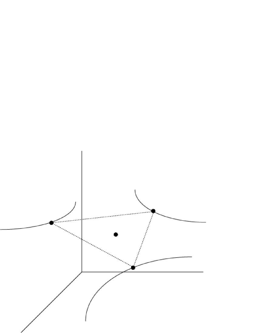
Figure 3.1: The dashed triangle outlines the convex hull of $x_{1}$, $x_{2}$, and $x_{3}$, shown as dots at the triangle’s vertices. This convex hull contains $\rho$, shown as a dot inside the triangle, and forms a (schematic) facet of $\mathcal{S}_{M,N}$. The curves represent the allowable choices for the $\tilde{x}_{i}$. Sliding any of the $x_{i}$ takes $\mathrm{conv}\{x_{1},x_{2},x_{3}\}$ outside of the facet.

Furthermore, even if $x_{i}$ can be nudged comfortably to a rational $\tilde{x}_{i}$, one would have to prove that $<\tilde{x}_{i}>\in O(\text{poly}(<[\rho]>))$, where $<X>$ is the size of the encoding of $X$.

So, either the definition of NP does not apply (for weak membership formulations), or we possibly run into problems near the boundary of $\mathcal{S}_{M,N}$ (for exact formulations). Below we give an alternative formulation that is in NP; we will refer to this problem as QSEP. The definition of QSEP is just a precise formulation of the question “Given a density operator $\rho$, does there exist a separable density operator $\hat{\sigma}$ that is close to $\rho$?” We must choose a guess-and-check procedure on which to base QSEP. Because I want to prove that QSEP is NP-hard, it is easier to choose the procedure which has the less complex check (but the larger guess).

Definition 16 (QSEP).

Given a rational density matrix $[\rho]$ of dimension $MN$-by-$MN$, and positive rational numbers $\delta_{p}$, $\epsilon^{\prime}$ and $\delta^{\prime}$; does there exist a distribution $\{(\tilde{p}_{i};\tilde{\alpha}_{i},\tilde{\beta}_{i})\}_{i=1,2,...,M^{2}N^{2}}$ of unnormalised pure states $\tilde{\alpha}_{i}\in\mathbb{C}^{M}$, $\tilde{\beta}_{i}\in\mathbb{C}^{N}$ where $\tilde{p}_{i}\geq 0$, and $\tilde{p}_{i}$ and all elements of $\tilde{\alpha}_{i}$ and $\tilde{\beta}_{i}$ are $\lceil\log_{2}(1/\delta_{p})\rceil$-bit numbers (complex elements are $x+iy$, $x,y\in\mathbb{R}$; where $x$ and $y$ are $\lceil\log_{2}(1/\delta_{p})\rceil$-bit numbers) such that

$$|1-||\tilde{\alpha}_{i}||^{2}||\tilde{\beta}_{i}||^{2}\sum_{j=1}^{M^{2}N^{2}}\tilde{p}_{j}|<\epsilon^{\prime}\hskip 14.22636pt\textrm{for all $i$}$$ (3.17)

and

$$||[\rho]-\tilde{\sigma}||^{2}_{2}:=\textrm{tr}(([\rho]-\tilde{\sigma})^{2})<\delta^{\prime 2},$$ (3.18)

where $\tilde{\sigma}:=\sum_{i=1}^{M^{2}N^{2}}\tilde{p}_{i}\tilde{\alpha}_{i}\tilde{\alpha}_{i}^{\dagger}\otimes\tilde{\beta}_{i}\tilde{\beta}_{i}^{\dagger}$?

Note that these checks can be done exactly in polynomial-time, as they only involve elementary arithmetic operations on rational numbers. To reconcile this definition with the above intuition, we define $\hat{\sigma}$ as the separable density matrix that is the “normalised version” of $\tilde{\sigma}$:

$$\hat{\sigma}:=\sum_{i=1}^{M^{2}N^{2}}\hat{p}_{i}\hat{\alpha}_{i}\hat{\alpha}_{i}^{\dagger}\otimes\hat{\beta}_{i}\hat{\beta}_{i}^{\dagger},$$ (3.19)

where $\hat{p}_{i}:=\tilde{p}_{i}/\sum_{i}\tilde{p}_{i}$, $\hat{\alpha}_{i}:=\tilde{\alpha}_{i}/||\tilde{\alpha}_{i}||$, and $\hat{\beta}_{i}:=\tilde{\beta}_{i}/||\tilde{\beta}_{i}||$. Using the triangle inequality, we can derive that

$$||\hat{\sigma}-\tilde{\sigma}||_{2}\leq\sum_{i}\hat{p}_{i}|1-||\tilde{\alpha}_{i}||^{2}||\tilde{\beta}_{i}||^{2}\sum_{j}\tilde{p}_{j}|,$$ (3.20)

where the righthand side is less than $\epsilon^{\prime}$ when (3.17) is satisfied. If (3.18) is also satisfied, then we have

$$||[\rho]-\hat{\sigma}||_{2}\leq||[\rho]-\tilde{\sigma}||_{2}+||\hat{\sigma}-\tilde{\sigma}||_{2}\leq\delta^{\prime}+\epsilon^{\prime},$$ (3.21)

which says that the given $[\rho]$ is no further than $\delta^{\prime}+\epsilon^{\prime}$ away from a separable density matrix (in Euclidean norm).

The decision problem QSEP is trivially in NP, as a nondeterministic Turing machine need only guess the $\lceil\log_{2}(1/\delta_{p})\rceil$-bit distribution $\{(\tilde{p}_{i};\tilde{\alpha}_{i},\tilde{\beta}_{i})\}_{i=1,2,...,M^{2}N^{2}}$ and verify (in polytime) that (3.17) and (3.18) are satisfied.

3.2.3 NP-Hardness

Gurvits [67] has shown the weak membership problem for $\mathcal{S}_{M,N}$ to be NP-hard with respect to the complexity-measure $(N+<[\rho]>+<\delta>)$. He demonstrates a Turing-reduction from PARTITION and makes use of the very powerful Yudin-Nemirovskii theorem (Theorem 4.3.2 in [1]).

We check now that QSEP is NP-hard, by way of a Karp-reduction from WMEM($\mathcal{S}_{M,N}$). We assume we are given an instance $I:=([\rho],\delta)$ of WMEM($\mathcal{S}_{M,N}$) and we seek an instance $I^{\prime}:=([\rho^{\prime}],\delta_{p},\epsilon^{\prime},\delta^{\prime})$ of QSEP such that if $I^{\prime}$ is a “yes”-instance of QSEP, then $I$ satisfies (3.3); otherwise $I$ satisfies (3.4). It suffices to use $[\rho^{\prime}]=[\rho]$. It is clear that if $\delta^{\prime}$ and $\epsilon^{\prime}$ are chosen such that $\delta\geq\delta^{\prime}+\epsilon^{\prime}$, then $I^{\prime}$ is a “yes”-instance only if $I$ satisfies (3.3). For the other implication, we need to bound the propagation of some truncation-errors. Let $p:=\lceil\log_{2}(1/\delta_{p})\rceil$.

Recall how absolute errors accumulate when multiplying and adding numbers. Let $x=\tilde{x}+\Delta_{x}$ and $y=\tilde{y}+\Delta_{y}$ where $x$, $y$, $\tilde{x}$, $\tilde{y}$, $\Delta_{x}$, and $\Delta_{y}$ are all real numbers. Then we have

$$xy = \tilde{x}\tilde{y}+\tilde{x}\Delta_{y}+\tilde{y}\Delta_{x}+\Delta_{x}\Delta_{y}$$ (3.22)

$$x+y = \tilde{x}+\tilde{y}+\Delta_{x}+\Delta_{y}.$$ (3.23)

For $|\tilde{x}|,|\tilde{y}|<1$, because we will be dealing with summations of products with errors, it is sometimes convenient just to use

$$|xy-\tilde{x}\tilde{y}| \leq |\Delta_{y}|+|\Delta_{x}|+\textrm{max}\{|\Delta_{x}|,|\Delta_{y}|\}$$ (3.24)

to obtain our cumulative errors (which do not need to be tight to show NP-hardness). For example, if $\tilde{x}$ and $\tilde{y}$ are the $p$-bit truncations of $x$ and $y$, where $|x|,|y|<1$, then $|\Delta_{x}|,|\Delta_{y}|<2^{-p}$; thus a conservative bound on the error of $\tilde{x}\tilde{y}$ is

$$|xy-\tilde{x}\tilde{y}|<|\Delta_{y}|+|\Delta_{x}|+|\Delta_{x}|=3|\Delta_{x}|<2^{2}|\Delta_{x}|=2^{-(p-2)}.$$

Proposition 6.

Let $\sigma\in\mathcal{S}_{M,N}$ be such that $\sigma=\sum_{i=1}^{M^{2}N^{2}}p_{i}\alpha_{i}\alpha_{i}^{\dagger}\otimes\beta_{i}\beta_{i}^{\dagger}$, and let
$\{(\tilde{p}_{i};\tilde{\alpha}_{i},\tilde{\beta}_{i})\}_{i=1,2,...,M^{2}N^{2}}$ be the $p$-bit truncation of $\{({p}_{i};{\alpha}_{i},{\beta}_{i})\}_{i=1,2,...,M^{2}N^{2}}$.
Then $||\sigma-\tilde{\sigma}||_{2}<M^{3}N^{3}2^{-(p-7.5)}$, where

$$\tilde{\sigma}:=\sum_{i=1}^{M^{2}N^{2}}\tilde{p}_{i}\tilde{\alpha}_{i}\tilde{\alpha}_{i}^{\dagger}\otimes\tilde{\beta}_{i}\tilde{\beta}_{i}^{\dagger}.$$ (3.25)

Proof.

Letting $\gamma_{i}:=p_{i}\alpha_{i}\alpha_{i}^{\dagger}\otimes\beta_{i}\beta_{i}^{\dagger}-\tilde{p}_{i}\tilde{\alpha}_{i}\tilde{\alpha}_{i}^{\dagger}\otimes\tilde{\beta}_{i}\tilde{\beta}_{i}^{\dagger}$, we use the triangle inequality to get

$$||\sigma-\tilde{\sigma}||_{2} \leq \sum_{i}||\gamma_{i}||_{2}=\sum_{i}\sqrt{\textrm{tr}(\gamma_{i}^{2})}.$$ (3.26)

It suffices to bound the absolute error on the elements of $[\tilde{p}_{i}\tilde{\alpha}_{i}\tilde{\alpha}_{i}^{\dagger}\otimes\tilde{\beta}_{i}\tilde{\beta}_{i}^{\dagger}]$; using our conservative rule (3.24), these elements have absolute error less than $2^{-(p-7)}$. Thus $[\gamma_{i}]$ is an $MN$-by-$MN$ matrix with elements no larger than $2^{-(p-7)}$ in absolute value. It follows that $(\textrm{tr}(\gamma_{i}^{2}))^{1/2}$ is no larger than $\sqrt{MN}2^{-(p-7.5)}$ in absolute value. Finally, we get

$$||\sigma-\tilde{\sigma}||_{2}\leq\sum_{i}\sqrt{\textrm{tr}(\gamma_{i}^{2})}\leq M^{3}N^{3}2^{-(p-7.5)}.$$ (3.27)

∎

Proposition 7.

Let $\tilde{\sigma}$ be as in Proposition 6. Then for all $i=1,2,\ldots M^{2}N^{2}$

$$|1-||\tilde{\alpha}_{i}||^{2}||\tilde{\beta}_{i}||^{2}\sum_{j=1}^{M^{2}N^{2}}\tilde{p}_{j}|<M^{3}N^{3}2^{-(p-5)}.$$ (3.28)

Proof.

The absolute error on $\sum_{j}\tilde{p}_{j}$ is $M^{2}N^{2}2^{-p}$. The absolute error on $||\tilde{\alpha}_{i}||^{2}$ (resp. $||\tilde{\beta}_{i}||^{2}$) is no more than $M2^{-(p-3)}$ (resp. $N2^{-(p-3)}$). This gives total absolute error of

$$|1-{||\tilde{\alpha}_{i}||^{2}||\tilde{\beta}_{i}||^{2}}\sum_{j}\tilde{p}_{j}|<M^{3}N^{3}2^{-(p-5)}.$$ (3.29)

∎

Let $\delta^{\prime}:=M^{3}N^{3}2^{-(p-8)}$ and $\epsilon^{\prime}:=M^{3}N^{3}2^{-(p-5)}$ and set $p$ such that $\epsilon^{\prime}+\delta^{\prime}\leq\delta$. Suppose there exists a separable density matrix $\sigma$ such that $||[\rho]-\sigma||_{2}=0$. Then Propositions 6 and 7 say that there exists a certificate $\tilde{\sigma}$ such that (3.17) and (3.18) are satisfied. Therefore, if $I^{\prime}$ is a “no”-instance, then for all separable density matrices $\sigma$, $||[\rho]-\sigma||_{2}>0$; which implies that $I$ satisfies (3.4). I have exhibited a polytime Karp-reduction from WMEM($\mathcal{S}_{M,N}$) to QSEP (actually, from $\text{WMEM}_{\text{In}}(\mathcal{S}_{M,N})$ to QSEP).

Fact 8.

QSEP is in $\mathrm{NPC_{\mathrm{T}}}$.

3.2.4 Towards a Karp Reduction

To date, every decision problem (except for QSEP) that is in $\mathrm{NPC_{\mathrm{T}}}$ is also known to be in $\mathrm{NPC_{\mathrm{K}}}$ [72]. While it is strongly suspected that Karp and Turing reductions are inequivalent within NP, it would be very strange if QSEP, or some other formulation of the quantum separability problem, is the first example that proves this inequivalence. We have an interesting open problem:

Problem 4.

Is QSEP in $\mathrm{NPC_{\mathrm{K}}}$?

Note that, because of Fact 8, a negative answer to this problem implies that $\mathrm{P}\neq\mathrm{NP}$. Thus it might be safer to work under the assumption that the answer is positive, and look for a Karp reduction from some Karp-NP-complete problem to some formulation $\Pi_{\mathrm{QSEP}}$ of the quantum separability problem.

Technically, WMEM($\mathcal{S}_{M,N}$) is not in NP because it is not a decision problem. But the definition of “NP” can be modified to accommodate such weakened problems having overlapping decisions [1]. According to this different definition, WMEM($\mathcal{S}_{M,N}$) is in “NP”. We can pose the following open problem, related to the one above.

Problem 5.

Does there exist a Karp reduction from some Karp-NP-complete problem to WMEM($\mathcal{S}_{M,N}$)?

Finding a positive answer to this problem implies a positive answer for Problem 4. Alternatively, finding a negative answer to this problem does not, technically, imply that $\mathrm{P}\neq\mathrm{NP}$, so may not win the million-dollar prize.

3.2.5 Nonmembership in co-NP

Is either EXACT QSEP or QSEP in co-NP? To avoid possible technicalities, we might first consider the presumably easier question of whether WMEM($\mathcal{S}_{M,N}$) is in “co-NP”: Does every entangled state $\rho\notin S(\mathcal{S}_{M,N},\delta)$ have a succinct certificate of not being in $S(\mathcal{S}_{M,N},-\delta)$? It may or may not be the case that P equals NP$\cap$co-NP, but a problem’s membership in NP$\cap$co-NP can be “regarded as suggesting” that the problem is in P [70]. Thus, we might believe that WMEM($\mathcal{S}_{M,N}$) is not in “co-NP” (since WMEM($\mathcal{S}_{M,N}$) is NP-hard).

Let us consider this with regard to entanglement witnesses (which are candidates for succinct certificates of entanglement). We know that every entangled state has a (right) entanglement witness $A\in\mathbb{H}_{M,N}$ that detects it. However, it follows from the NP-hardness of WMEM($\mathcal{S}_{M,N}$) and Theorem 4.4.4 in [1] that the weak validity problem for $K=\mathcal{S}_{M,N}$ (WVAL($\mathcal{S}_{M,N}$)) is NP-hard:

Definition 17 (Weak validity problem (WVAL)).

Given a rational vector $c\in\mathbb{R}^{n}$, a rational number $\gamma$, and rational $\epsilon>0$, assert either that

$$c^{T}x \leq \gamma+\epsilon\text{ for all }x\in K,\hskip 5.69054pt\text{or}$$ (3.30)

$$c^{T}x \geq \gamma-\epsilon\text{ for some }x\in K.$$ (3.31)

So there is no known way to check efficiently that a hyperplane $\pi_{A,b}$ separates $\rho$ from $\mathcal{S}_{M,N}$ (given just the hyperplane); thus, an entanglement witness alone does not serve as a succinct certificate of a state’s entanglement unless WVAL($\mathcal{S}_{M,N}$) is in P. However, one could imagine that there is a succinct certificate of the fact that a hyperplane $\pi_{A,b}$ separates $\rho$ from $\mathcal{S}_{M,N}$. If such a certificate exists, then WVAL($\mathcal{S}_{M,N}$) is in “NP” and WMEM($\mathcal{S}_{M,N}$) is in “co-NP”.

With regard to QSEP, we can prove the following:

Fact 9.

QSEP is not in co-NP, unless NP equals co-NP.

This fact follows from the general theorem below [73]:

Theorem 10.

If $\Pi$ is in $\mathrm{NPC_{\mathrm{T}}}$ and $\Pi$ is in co-NP, then NP equals co-NP.

Proof.

Since $\Pi$ is in co-NP, $\Pi^{c}$ is in NP. Let $\Pi^{\prime}$ be any problem in co-NP. To show that co-NP equals NP, it suffices to show that co-NP is contained in NP; thus, it suffices to show that $\Pi^{\prime}$ is in NP. The following reduction chain holds, since $\Pi^{\prime c}$ is in NP: $\Pi^{\prime}\leq_{\mathrm{T}}\Pi^{\prime c}\leq_{\mathrm{T}}\Pi$. Because both $\Pi$ and $\Pi^{c}$ are in NP, the reduction $\Pi^{\prime}\leq_{\mathrm{T}}\Pi$ can be carried out by a polytime nondeterministic Turing machine, which can “solve” any query to $\mathcal{O}_{\Pi}$ by nondeterministically guessing and checking in polynomial-time the “yes”-certificate (if the query is a “yes”-instance of $\Pi$) or the “no”-certificate (if the query is a “no”-instance of $\Pi)$. Thus $\Pi^{\prime}$ is in NP. ∎

It is strongly conjectured that NP and co-NP are different [69], thus we might believe that QSEP is not in co-NP.

3.3 Survey of algorithms for the quantum separability problem

I concentrate on proposed algorithms that solve an approximate formulation of the quantum separability problem and have (currently known) asymptotic analytic bounds on their running times. For this reason, the SDP relaxation algorithm of Eisert et al. is not mentioned here (see Section 1.3.2); though, I do not mean to suggest that in practice it could not outperform the following algorithms on typical instances. As well, I do not analyse the complexity of the naive implementation of every necessary and sufficient criterion for separability, as it is assumed that this would yield algorithms of higher complexity than the following algorithms.

The main purpose below is to get a time-complexity estimate in terms of the parameters $M$, $N$, and $\delta$, where $\delta$ is the accuracy parameter in WMEM($\mathcal{S}_{M,N}$). In the following, the only way precision and error are dealt with is similar to the above discussion, where we have a truncation-error resulting from approximating the continuum of pure product states by a finite set of finitely precise product vectors. The running-time estimates are based on the number of elementary arithmetic operations and do not attempt to deal with computer round-off error; I do not give estimates on the total amount of machine precision required. Instead, where rounding is necessary in order to avoid exponential blow-up of the representation of numbers during the computation, I assume that the working precision can be set large enough that the overall effect of the round-off error on the final answer is either much smaller than $\delta$ or no larger than, say, $\delta/2$ (so that doubling $\delta$ takes care of the error due to round-off).

3.3.1 Search for separable decompositions

The most naive algorithm for any problem in NP consists of a search through all potential succinct certificates that the given problem instance is a “yes”-instance. Thus QSEP immediately gives an algorithm for the quantum separability problem. However, we can, in principle, reformulate QSEP to incorporate the ideas of Hulpke and Bruß [60] in order to get a better algorithm.

The algorithm of Hulpke and Bruß

First, let us see how to perform the checks in lines (3.15) and (3.16). Using simpler notation, suppose we are given $\{x_{i}:\hskip 5.69054pti=1,2,\ldots,k\}\subset\mathbb{R}^{n}$. This set is affinely independent if and only if $\{x_{i}-x_{1}:\hskip 5.69054pti=2,\ldots,k\}$ is linearly independent. Thus Gaussian elimination can be used to test for affine independence. Suppose $\{x_{i}:\hskip 5.69054pti=1,2,\ldots,n+1\}$ is affinely independent. Then the $x_{i}$ form the extreme points of the polytope $\mathrm{conv}\{x_{i}:\hskip 5.69054pti=1,2,\ldots,n+1\}$. Consider the facet of this polytope that does not contain $x_{j}$, and choose some $x_{l}\neq x_{j}$ in the facet. The normal $\nu_{j}$ to this facet is orthogonal to $x_{i}-x_{l}$, for all $i\neq j,l$, and is thus the generator of the nullspace of the matrix whose $n-1$ rows are the vectors $x_{i}-x_{l}$. Again, Gaussian elimination can be used to solve for $\nu_{j}$. A point $\rho$ is in the polytope if and only if, for all $j=1,2,\ldots,n+1$, the halfspace $\{x:\nu_{j}^{T}x\leq\nu_{j}^{T}x_{l}\}$ contains both or neither of $\rho$ and $x_{j}$; that is, both $\rho$ and $x_{j}$ are on the “same side” of the hyperplane $\{x:\nu_{j}^{T}x=\nu_{j}^{T}x_{l}\}$ corresponding to the facet not containing $x_{j}$.

The algorithm of Hulpke and Bruß is basically a loop through all possible affinely independent sets $X$ of pure product states, with the check for whether $\mathrm{conv}X$ contains the given state $\rho$. However, the algorithm uses unbounded precision and performs its calculations to arbitrarily high precision so that it attempts to find such (arbitrarily precise) $X$ for $\rho\in\mathcal{S}_{M,N}$ that are arbitrarily close to the boundary of $\mathcal{S}_{M,N}$; it may even find such $X$ for $\rho\in\mathcal{S}_{M,N}$ that are on the boundary of the “cone” of positive Hermitian operators and hence on the boundary of $\mathcal{S}_{M,N}$. The algorithm only relaxes and solves the weak membership problem for states $\rho\in\mathcal{S}_{M,N}$ that are on the boundary between separable and entangled states. As argued at the beginning of this chapter, we are satisfied with an algorithm for the weak membership problem for all states. Thus we will formulate an approximate version of this algorithm whose precision requirements for the $X$ are bounded by $M$, $N$, and $\delta$.

Reformulation of QSEP

Recall the mapping $v:\mathbb{H}_{M,N}\rightarrow\mathbb{R}^{M^{2}N^{2}-1}$ defined in (2.12) on page 2.12.

Definition 18 (QSEP’).

Given a rational density matrix $[\rho]$ of dimension $MN$-by-$MN$, and positive rational numbers $\delta_{p}$ and $\epsilon^{\prime}$; does there exist a set $\{(\tilde{\alpha}_{i},\tilde{\beta}_{i})\}_{i=1,2,...,M^{2}N^{2}}$ of unnormalised pure states $\tilde{\alpha}_{i}\in\mathbb{C}^{M}$, $\tilde{\beta}_{i}\in\mathbb{C}^{N}$ where all elements of $\tilde{\alpha}_{i}$ and $\tilde{\beta}_{i}$ are $\lceil\log_{2}(1/\delta_{p})\rceil$-bit numbers (complex elements are $x+iy$, $x,y\in\mathbb{R}$; where $x$ and $y$ are $\lceil\log_{2}(1/\delta_{p})\rceil$-bit numbers) such that

$$|1-||\tilde{\alpha}_{i}||^{2}||\tilde{\beta}_{i}||^{2}|<\epsilon^{\prime}\hskip 14.22636pt\textrm{for all $i$}$$ (3.32)

and

$$\{v(\tilde{\alpha}_{i}\tilde{\alpha}_{i}^{\dagger}\otimes\tilde{\beta}_{i}\tilde{\beta}_{i}^{\dagger})\}_{i}\text{ is affinely independent}$$ (3.33)

and

$$[\rho]\in S(\mathrm{conv}\{v(\tilde{\alpha}_{i}\tilde{\alpha}_{i}^{\dagger}\otimes\tilde{\beta}_{i}\tilde{\beta}_{i}^{\dagger})\}_{i},\epsilon^{\prime})?$$ (3.34)

Note that (3.32) ensures that $\tilde{\alpha}_{i}\tilde{\alpha}_{i}^{\dagger}\otimes\tilde{\beta}_{i}\tilde{\beta}_{i}^{\dagger}$ is $\epsilon^{\prime}$-close to an actual state $\hat{\alpha}_{i}\hat{\alpha}_{i}^{\dagger}\otimes\hat{\beta}_{i}\hat{\beta}_{i}^{\dagger}$, where $\hat{\alpha}_{i}:=\tilde{\alpha}_{i}/||\tilde{\alpha}||$ and $\hat{\beta}_{i}:=\tilde{\beta}_{i}/||\tilde{\beta}||$. The check in line (3.34) is an easy modification of the check described in the previous subsection. Let $p:=\lceil\log_{2}(1/\delta_{p})\rceil$.

Suppose that, for some $\sigma\in\mathcal{S}_{M,N}$, $\sigma\in\mathrm{conv}\{\alpha_{i}\alpha_{i}^{\dagger}\otimes\beta_{i}\beta_{i}^{\dagger}\}_{i=1}^{M^{2}N^{2}-1}$ for normalised pure states $\alpha_{i}\in\mathbb{C}^{M}$ and $\beta_{i}\in\mathbb{C}^{N}$. Let $\tilde{\alpha}_{i}$ and $\tilde{\beta}_{i}$ be the $p$-bit truncations of $\alpha_{i}$ and $\beta_{i}$, and let $\gamma_{i}:=\alpha_{i}\alpha_{i}^{\dagger}\otimes\beta_{i}\beta_{i}^{\dagger}-\tilde{\alpha}_{i}\tilde{\alpha}_{i}^{\dagger}\otimes\tilde{\beta}_{i}\tilde{\beta}_{i}^{\dagger}$. The rectangular coordinates of the entries in $[\gamma_{i}]$ are no bigger than $2^{-(p-6)}$. It follows that $\sqrt{\textrm{tr}(\gamma_{i}^{2})}$ is not larger than $MN2^{-(p-6.5)}$:

$$||\alpha_{i}\alpha_{i}^{\dagger}\otimes\beta_{i}\beta_{i}^{\dagger}-\tilde{\alpha}_{i}\tilde{\alpha}_{i}^{\dagger}\otimes\tilde{\beta}_{i}\tilde{\beta}_{i}^{\dagger}||\leq MN2^{-(p-6.5)}.$$ (3.35)

Thus, setting $\epsilon^{\prime}:=MN2^{-(p-7)}$ and setting $p$ such that $2\epsilon^{\prime}<\delta$, it follows that QSEP’ solves WMEM($\mathcal{S}_{M,N}$) with accuracy parameter $\delta$. This gives

$$p>\log_{2}(2MN/\delta)+7.$$ (3.36)

Therefore, to solve WMEM($\mathcal{S}_{M,N}$), it suffices to loop through all $(M^{2}N^{2})$-subsets of $\lceil\log_{2}(2MN/\delta)+7\rceil$-bit unnormalised pure product states, checking the three conditions in QSEP’. Define $\Omega_{p}$ as the number of $p$-bit unnormalised pure product states resulting from the truncation (to $p$ bits) of all normalised pure product states. The complexity of this algorithm is

$$\left(\!\begin{array}[]{c}\Omega_{\lceil\log_{2}(2MN/\delta)+7\rceil}\\ M^{2}N^{2}\end{array}\!\right)\text{poly}(M,N,\log(1/\delta)).$$ (3.39)

Since the pure product states can be parametrised by $2(M+N)-4$ real parameters, we have the estimate

$$\Omega_{p}\gtrsim 2^{p(2(M+N)-4)}.$$ (3.40)

Combined with the estimate $\left(\!\begin{array}[]{c}n\\ k\end{array}\!\right)\sim n^{k}$, we get a rough asymptotic complexity estimate for the algorithm of

$$\left(\frac{2^{6.5}MN}{\delta}\right)^{2(M^{3}N^{2}+M^{2}N^{3})-4M^{2}N^{2}}\text{poly}(M,N,\log(1/\delta)).$$ (3.41)

In the interest of getting a rough lower bound on the complexity of this algorithm, I have underestimated $\Omega_{p}$. The number $2^{p(2(M+N)-4)}$ corresponds to the number of different $p$-bit settings of the $2(M+N)-4$ angles (phases and amplitudes) that parametrise the normalised pure product states. The truncation-error analysis was done with respect to rectangular coordinates, so this method of generating the elements $\tilde{\alpha}_{j}\otimes\tilde{\beta}_{j}$ may miss some elements that would have resulted from a $p$-bit truncation of rectangular coordinates of normalised pure product states. On the other hand, if we use all $p$-bit settings of the $2(M+N)$ rectangular coordinates to generate elements $\tilde{\alpha}_{j}\otimes\tilde{\beta}_{j}$, then many of the elements generated will not satisfy $|1-||\tilde{\alpha}_{j}||^{2}||\tilde{\beta}_{j}||^{2}|<\epsilon^{\prime}$. The most efficient way to systematically generate the elements $\tilde{\alpha}_{j}\otimes\tilde{\beta}_{j}$ is left as an open problem:

Problem 6.

What is the most efficient way to generate the $j$th element $\tilde{\alpha}_{j}\otimes\tilde{\beta}_{j}$ of the set of $\Omega_{p}$ unnormalised pure product states resulting from the $p$-bit truncation of all normalised pure product states?

We take the algorithm of this section as the best exhaustive search approach to solving the approximate quantum separability problem. For example, it is better than searching all of $\mathcal{S}_{M,N}$ in order to calculate $E_{d^{2}_{2}}(\rho)$ of Section 1.3.2; and it is better than searching all pure decompositions of $\rho$ in order to calculate $E^{\prime}_{F}(\rho)$ of Section 1.3.3.

3.3.2 Bounded search for symmetric extensions

In Section 1.3.1, we considered two tests – one that searches for symmetric extensions of $\rho$, and a stronger one that searches for PPT symmetric extensions. Now we continue that exposition, showing that recent results can put an upper bound on the number $k$ of copies of subsystem $\mathrm{A}$ when solving an approximate formulation of the separability problem. The bound only assumes symmetric extensions, not PPT symmetric extensions, so it is possible that a better bound may be found for the stronger test.

If a symmetric state $\varrho\in\mathcal{D}((\mathbb{C}^{d})^{\otimes n})$ has a symmetric extension to $\mathcal{D}((\mathbb{C}^{d})^{\otimes(n+m)})$ for all $m>0$, then it is called (infinitely) exchangeable. The quantum de Finetti theorem says that the infinitely exchangeable state $\varrho$ is separable. Recalling the terminology of Section 1.3.1, it is also possible to derive that, for $\rho\in\mathcal{D}(\mathbb{C}^{M}\otimes\mathbb{C}^{N})$, if there exists a symmetric extension of $\rho$ to $k$ copies of subsystem $\mathrm{A}$ for all $k>0$, then $\rho\in\mathcal{S}_{M,N}$. This is the result that proves that Doherty et al.’s hierarchy of tests is complete: if $\rho$ is entangled, then the SDP at some level $k_{0}$ of the hierarchy will not be feasible (i.e. will not find a symmetric extension of $\rho$ to $k_{0}$ copies of subsystem $\mathrm{A}$). König and Renner [75] derived quite general results about states $\rho$ that have symmetric extensions to $k$ copies of subsystem $\mathrm{A}$. Their results give us our upper bound on $k$.

The upper bound follows directly from the main theorem in [75]. The result is too technical to summarise meaningfully without diverging from the aim of this thesis. We require the following corollary:

Theorem 11 (Corollary of Theorem 6.1 in [75]).

Suppose $\rho\in\mathcal{D}_{M,N}$ and there exists a symmetric extension of $\rho$ to $k\geq 2$ copies of subsystem $\mathrm{A}$. Then

$$\textrm{tr}|\rho-\sigma|\leq\frac{4M^{6}}{\sqrt{k-1}},$$ (3.42)

for some $\sigma\in\mathcal{S}_{M,N}$.

The proof of this theorem is similar to the proof of Corollary 6.2 in [75]. Note that the result uses the trace distance, $\textrm{tr}|X-Y|$, between two operators $X$ and $Y$. Let us assume we are solving the weak membership formulation of the quantum separability problem with respect to the trace distance, and with accuracy parameter $\delta$. Then, setting $\delta={4M^{6}}/{\sqrt{k-1}}$, we get the following upper bound for $k$:

Corollary 12.

To solve WMEM($\mathcal{S}_{M,N}$) (with respect to the trace distance) with accuracy parameter $\delta$ by searching for symmetric extensions (as described in Section 1.3.1), it suffices to look for symmetric extensions to

$$\bar{k}:=\lceil 16M^{12}/\delta^{2}+1\rceil$$ (3.43)

copies of subsystem A.

To estimate the total complexity of the algorithm, note that

$$d_{S_{k}}=\frac{[(M-1)+k][(M-2)+k]\cdots[(1)+k]}{(M-1)!}>k^{M-1}/(M-1)!.$$ (3.44)

Substituting $\bar{k}$ for $k$, we get

$$d_{S_{\bar{k}}}>\left(\frac{16M^{11}}{\delta^{2}}\right)^{M-1}.$$ (3.45)

Just to solve the first constraint in (1.6) requires $\sqrt{n}$ (but usually far fewer) iterations of a procedure that requires $O(m^{2}n^{2})$ arithmetic operations, for $m=(d_{S_{\bar{k}}}^{2}-M^{2})N^{2}$ and $n=d_{S_{\bar{k}}}^{2}N^{2}$.

Problem 7.

Can the upper bound $\bar{k}$ be improved by taking into consideration the PPT constraints in (1.6)?

Despite this unattractive worst-case bound, the hierarchy of tests has proved to be efficient in practice for confirming that certain states are entangled (i.e. small $k$ suffices).

3.3.3 Cross-norm criterion via linear programming

Rudolph [76] derived a simple characterisation of separable states in terms of a computationally complex operator norm $||\cdot||_{\gamma}$. For a finite-dimensional vector space $V$, let $\mathcal{T}(V)$ be the class of all linear operators on $V$. The norm is defined on $\mathcal{T}(\mathbb{C}^{M})\otimes\mathcal{T}(\mathbb{C}^{N})$ as

$$||t||_{\gamma}:=\inf\{\sum_{i=1}^{k}||u_{i}||_{1}||v_{i}||_{1}:\hskip 2.84526ptt=\sum_{i=1}^{k}u_{i}\otimes v_{i}\},$$ (3.46)

where the infimum is taken over all decompositions of $t$ into finite summations of elementary tensors, and $||X||_{1}:=\textrm{tr}(\sqrt{X^{\dagger}X})$. Rudolph showed that $||\rho||_{\gamma}\leq 1$ if and only if $||\rho||_{\gamma}=1$, and that a state $\rho$ is separable if and only if $||\rho||_{\gamma}=1$.

Pérez-Garcia [77] showed that approximately computing this norm can be reduced to a linear program (which is a special case of a semidefinite program): $\min\{c^{T}x:\hskip 5.69054ptAx=b,x\geq 0\}$, where $A\in\mathbb{R}^{n\times m}$, $b\in\mathbb{R}^{n}$, $c\in\mathbb{R}^{m}$, and $x$ is a vector of $m$ real variables; here, $x\geq 0$ means that all entries in the vector are nonnegative. An LP can be solved in $O(m^{3}L^{\prime})$ arithmetic operations, where $L^{\prime}$ is the length of the binary encoding of the LP [78]. The linear program has on the order of $M^{2}N^{2}$ variables and $M^{2M}N^{2N}(2k)^{2(M+N)}$ constraints, where $k$ is an integer that determines the relative error $(k/(k-1))^{4}-1$ on the computation of the norm. Thus it may be solved in

$$O(M^{2M+2}N^{2N+2}(2k)^{2(M+N)})$$ (3.47)

arithmetic operations.

Suppose $||\rho||_{\gamma}$ is found to be no greater than $1+\eta$. Then, we would like to use $\eta$ to upper-bound the distance, with respect to either trace or Euclidean norm, from $\rho$ to $\mathcal{S}_{M,N}$. Unfortunately, we do not know how to do this. This drawback, along with the fact that the error on the computed norm is relative as opposed to absolute, does not allow this algorithm to be easily compared to the other algorithms I consider. Still, there may be a way to overcome this problem, as follows.

Following Rudolph [12], a norm closely related to $||\cdot||_{\gamma}$ is

$$||t||_{\mathcal{S}}:=\inf\{\sum_{i=1}^{k}||u_{i}||_{1}||v_{i}||_{1}:\hskip 2.84526ptt=\sum_{i=1}^{k}u_{i}\otimes v_{i}\},$$ (3.48)

where the infimum is taken over all decompositions of $t$ into finite summations of elementary Hermitian tensors. This restriction on the decomposition implies that $||t||_{\gamma}\leq||t||_{\mathcal{S}}$; thus, if $||\rho||_{\mathcal{S}}\leq 1$, then $\rho\in\mathcal{S}_{M,N}$. Conversely, if $\rho\in\mathcal{S}_{M,N}$, then $\rho=\sum_{i}(p_{i}\rho^{\mathrm{A}}_{i})\otimes\rho^{\mathrm{B}}_{i}$; and this decomposition ensures $||\rho||_{\mathcal{S}}\leq 1$. Thus $||\rho||_{\mathcal{S}}\leq 1$ if and only if $\rho\in\mathcal{S}_{M,N}$. The norm $||\cdot||_{\mathcal{S}}$ is related to an entanglement measure called “robustness”.

The robustness of entanglement [18] of $\rho\in\mathcal{D}_{M,N}$ is defined as

$$R(\rho):=\inf\{a^{-}:\hskip 5.69054pt\rho=a^{+}\sigma^{+}-a^{-}\sigma^{-},\hskip 2.84526pta^{\pm}\geq 0,\sigma^{\pm}\in\mathcal{S}_{M,N}\}.$$ (3.49)

In other words, the robustness is (a simple function of) the minimal $p$, $0\leq p\leq 1$, such that

$$\sigma^{+}=p\sigma^{-}+(1-p)\rho$$ (3.50)

for separable states $\sigma^{\pm}$; the minimal $p$ is $p_{R(\rho)}:=R(\rho)/(R(\rho)+1)$. Thus, $R(\rho)$ corresponds to the minimal amount of separable “noise” ($\sigma^{-}$) that must be added to $\rho$ in order to eliminate all the entanglement in $\rho$.

Using properties of “subcross norms” (see references in [12]), Rudolph shows [12] that for $\rho\in\mathcal{D}_{M,N}$

$$R(\rho)\equiv\frac{1}{2}(||\rho||_{\mathcal{S}}-1);$$ (3.51)

the proof is based on the ideas of “base norm” used in [79].

The point is that if we could modify Pérez-Garcia’s algorithm so that it approximately computes $||\cdot||_{\mathcal{S}}$, then we could relate the result to a standard norm, as follows. Suppose the algorithm allows us to assert that $||\rho||_{\mathcal{S}}\leq 1+2\eta$. Then $R(\rho)\leq\eta$. Now, we have

$$||\rho-\sigma^{+}|| = ||p_{R(\rho)}(\rho-\sigma^{-})||$$ (3.52)

$$= p_{R(\rho)}||\rho-\sigma^{-}||$$ (3.53)

$$= \frac{R(\rho)}{1+R(\rho)}||\rho-\sigma^{-}||$$ (3.54)

$$\leq \frac{2\eta}{1+\eta},$$ (3.55)

where 2 is a an upper bound on the Euclidean diameter of the set of (normalised) density operators (see Figure 5.4 on page 5.4).

Problem 8.

Can the algorithm of Pérez-Garcia be modified so that it approximately computes the norm $||\cdot||_{\mathcal{S}}$?

Continuing with our hypothetical run-time analysis, how would we assert $||\rho||_{\mathcal{S}}\leq 1+2\eta$? The actual algorithm returns an approximation $x$ such that $||\rho||_{\gamma}\leq x\leq(k/(k-1))^{4}||\rho||_{\gamma}$. Let us assume that a modification of the algorithm which computes $||\rho||_{\mathcal{S}}$ would do the same. If the modified algorithm returns a number that is less than 1, then we know that $||\rho||_{\mathcal{S}}\leq 1$. Otherwise, all that we need is an upper bound $\mathrm{Abs}$ on the absolute error of the computation of $||\rho||_{\mathcal{S}}$, since, if $\mathrm{Abs}\leq\eta$, then we can comfortably conclude that either $||\rho||_{\mathcal{S}}\leq 1+2\eta$, or $||\rho||_{\mathcal{S}}>1$. Using the canonical basis $\mathcal{B}$ of $\mathbb{H}_{M,N}$ described in Section 2.3, we have $\mathrm{Max}:=\max_{\rho\in\mathcal{D}_{M,N}}||\rho||_{\mathcal{S}}\in O(\text{poly}(M,N))$, which says the absolute error $||\rho||_{\mathcal{S}}((k/(k-1))^{4}-1)$ is upper-bounded by $\mathrm{Abs}\in O(((k/(k-1))^{4}-1)\text{poly}(M,N))$. The requirement $\mathrm{Abs}<\eta$ leads to a lower bound for $k$ of

$$k>\frac{\mathrm{Max}^{1/4}}{(\eta+\mathrm{Max})^{1/4}-\mathrm{Max}^{1/4}}.$$ (3.56)

Rudolph [12] has also shown that, for $\rho\in\mathcal{D}_{M,N}$,

$$R(\rho)\geq||\rho||_{\gamma}-1.$$ (3.57)

If equality holds in equation (3.57), then an argument similar to the one above could be used. Rudolph notes that equality holds for pure states and “Werner” and “isotropic” states (see [79]).

3.3.4 Fixed-point iterative method

Zapatrin [80] suggests an iterative method that solves the separability problem. He defines the function $\Phi:\mathbb{H}_{M,N}\rightarrow\mathbb{H}_{M,N}$:

$$\Phi(X):=X+\lambda\left(\rho-\int\int e^{\left<\psi^{\mathrm{A}}\right|\otimes\left<\psi^{\mathrm{B}}\right|X\left|\psi^{\mathrm{A}}\right>\otimes\left|\psi^{\mathrm{B}}\right>}|\psi^{\mathrm{A}}\rangle\langle\psi^{\mathrm{A}}|\otimes|\psi^{\mathrm{B}}\rangle\langle\psi^{\mathrm{B}}|d\mathbf{S}_{M}d\mathbf{S}_{N}\right),$$ (3.60)

where $\mathbf{S}_{M}$ and $\mathbf{S}_{N}$ are the complex origin-centred unit spheres (containing, respectively, $\left|\psi^{\mathrm{A}}\right>$ and $\left|\psi^{\mathrm{B}}\right>$), and $\lambda$ is a constant dependent on the derivative (with respect to $X$) of the quantity in parentheses ($\lambda$ is chosen so that $\Phi$ is a contraction mapping). In earlier work [81, 82, 83], Zapatrin proves that any state $\sigma$ in the interior $\mathcal{S}_{M,N}^{\circ}$ of $\mathcal{S}_{M,N}$ may be expressed

$$\sigma=\int\int e^{\left<\psi^{\mathrm{A}}\right|\otimes\left<\psi^{\mathrm{B}}\right|X_{\sigma}\left|\psi^{\mathrm{A}}\right>\otimes\left|\psi^{\mathrm{B}}\right>}|\psi^{\mathrm{A}}\rangle\langle\psi^{\mathrm{A}}|\otimes|\psi^{\mathrm{B}}\rangle\langle\psi^{\mathrm{B}}|d\mathbf{S}_{M}d\mathbf{S}_{N}\in\mathcal{S}_{M,N},$$ (3.61)

for some Hermitian $X_{\sigma}$. Thus the function $\Phi$ has a fixed point $X_{\rho}=\Phi(X_{\rho})$ if and only if $\rho\in\mathcal{S}_{M,N}^{\circ}$. When $\rho\in\mathcal{S}_{M,N}^{\circ}$, then a neighbourhood (containing $0$) in the domain of $\Phi$ can be found where iterating $X_{i+1}:=\Phi(X_{i})$, starting at $X_{0}:=0$, will produce a sequence $(X_{i})_{i}$ that converges to $X_{\rho}$ when $\rho\in\mathcal{S}_{M,N}^{\circ}$, but diverges otherwise.

Each evaluation of $\Phi(X)$ requires $M^{2}N^{2}/2+MN$ integrations of the form

$$\int\int e^{\left<\psi^{\mathrm{A}}\right|\otimes\left<\psi^{\mathrm{B}}\right|X\left|\psi^{\mathrm{A}}\right>\otimes\left|\psi^{\mathrm{B}}\right>}\left<\textbf{e}^{\mathrm{A}}_{j}|\psi^{\mathrm{A}}\right>\left<\textbf{e}^{\mathrm{B}}_{j^{\prime}}|\psi^{\mathrm{B}}\right>\left<\psi^{\mathrm{A}}|\textbf{e}^{\mathrm{A}}_{k}\right>\left<\psi^{\mathrm{B}}|\textbf{e}^{\mathrm{B}}_{k^{\prime}}\right>d\mathbf{S}_{M}d\mathbf{S}_{N},$$ (3.62)

where $\{\textbf{e}^{\mathrm{A}}_{j}\}_{j}$ and $\{\textbf{e}^{\mathrm{B}}_{k}\}_{k}$ are the standard bases for $\mathbb{C}^{M}$ and $\mathbb{C}^{N}$. However, the off-diagonal ($j\neq k$, $j^{\prime}\neq k^{\prime}$) integrals have a complex integrand so are each really two real integrals; thus the total number of real integrations is $M^{2}N^{2}$. Let $\Xi_{\delta}$ represent the number of pure states at which the integrand needs to be evaluated in order to perform each real numerical integration, in order to solve the overall separability problem with accuracy parameter $\delta$. Zapatrin shows that the approximate number of iterations required is upper-bounded by $2N(N+1)L(\log(1/\delta),\log(N))$, where $L$ is a bilinear function of its arguments. The complexity of the entire algorithm is roughly (ignoring $\log(N)$ factors)

$$\Xi_{\delta}\text{poly}(M,N,\log(1/\delta)).$$ (3.63)

In numerical integration, the final result of the integration depends on the truncation-error at each point at which the integrand is numerically evaluated. This is detrimental to the complexity of Zapatrin’s algorithm and I just make the reasonable presumption that $\Xi_{\delta}$, whatever it is, is far greater than $\Omega_{p}$ in the other algorithms analysed in this thesis (for the same values of $M$, $N$, and $\delta$). I do not consider Monte-Carlo integration methods (i.e. methods based on random sampling), because randomised algorithms for the separability problem are outside our scope.

Chapter 4 Reduction to Entanglement Witness Search

In Section 3.3, we saw four proposed algorithms for solving an approximate formulation of the quantum separability problem, all of which have analytically bounded running times. This chapter introduces a fifth, which is based on the simple idea of searching for an entanglement witness for the given state. In the language of convex body problems set up in Chapter 3, it solves the in-biased weak separation problem for $K=\mathcal{S}_{M,N}$:

Definition 19 (In-biased weak separation problem ($\text{WSEP}_{\text{In}}$)).

Given a rational vector $p\in\mathbb{R}^{n}$ and rational $\delta>0$, either

• assert $p\in S(K,\delta)$,   or

• find a rational vector $c\in\mathbb{R}^{n}$ with $||c||_{\infty}=1$ such that $c^{T}x\leq c^{T}p$ for every $x\in K$.

Of the algorithms of the previous chapter, this fifth algorithm is most closely related, in spirit, to Zapatrin’s algorithm of Section 3.3.4. This is because both algorithms reduce the quantum separability problem to $\text{poly}(M,N,\log(1/\delta))$ iterations of a difficult function evaluation: in Zapatrin’s case, the difficulty is a numerical integration; in the following algorithm, the difficulty is the computation of a global maximum.

4.1 Overview

In Section 4.2, I explain that the quantum separability problem can be reduced to the computation of $b^{*}(A):=\max_{\sigma\in\mathcal{S}_{M,N}}\{\textrm{tr}(A\sigma)\}$ from Chapter 2. Recall that exactly computing $b^{*}(A)$ corresponds precisely to the strong optimisation problem for $K=\mathcal{S}_{M,N}$ (see Definition 7 on page 7). The main algorithm of this thesis (henceforth referred to as “the new algorithm”) is a new polynomial-time reduction from $\text{WSEP}_{\text{In}}(K)$ to the (weak) optimisation problem for $K$; the algorithm works for any convex set $K$ that satisfies certain conditions – not just $\mathcal{S}_{M,N}$. Section 4.3 explains how such an algorithm can be utilised in an experimental setting when faced with the problem of deciding whether an unknown state, of which many copies are available, is entangled; such an algorithm can be applied to give a one-sided test for separability even when only partial information about the state is available.

Recall that to solve $\text{WSEP}_{\text{In}}(\mathcal{S}_{M,N})$, in the case where the given state $\rho$ is entangled, means to provide a right entanglement witness that detects $\rho$. The new algorithm can be viewed as an exhaustive search for an entanglement witness for the given $\rho$; and if no entanglement witness is found, then the algorithm concludes that $\rho$ is close to separable. In Section 4.4, I give the basic idea behind the search method employed by the new algorithm. This search method is a variant of a well-known method in convex analysis, which I explain in Section 4.5. Both search methods yield oracle-polynomial-time reductions of the same asymptotic complexity. I discuss the general form of such reductions in Section 4.6. Indeed, the new algorithm is not an improvement on known reductions of its kind. The novelty of the work in this chapter, with regard to the quantum information processing community, is the discovery that the best known algorithm for the quantum separability problem (in the case $M=N$) is obtained by a reduction to the weak optimisation problem over $\mathcal{S}_{M,N}$: Section 4.7 gives an upper bound on the complexity of the weak optimisation problem over $\mathcal{S}_{M,N}$ and Section 4.8 contains the comparison of the complexities of the new algorithm and the algorithms of Sections 3.3.1 and 3.3.2. With regard to the convex programming community, the new algorithm (whose details are presented in Chapter 5) is a variant of well-known algorithms which, while perhaps not offering any computational advantage, arguably holds intrinsic beauty because it is based on a simple, intuitive heuristic (explained in Section 4.4).

4.2 Reduction to optimisation

Recall the function $b^{*}(A):=\max_{\sigma\in\mathcal{S}_{M,N}}\{\textrm{tr}(A\sigma)\}$ from Chapter 2. This function leads naturally to an algorithm for quantum separability as follows. For $A\in\mathbb{H}_{M,N}$ such that $tr(A^{2})=1$, define the function $d_{\rho}(A)$ as

$$d_{\rho}(A):=b^{*}(A)-tr(A\rho).$$ (4.1)

Geometrically, $d_{\rho}(A)$ is the signed distance from the state $\rho$ to the hyperplane $\pi_{A,b^{*}(A)}$. It follows that $\rho$ is entangled if and only if there exists an $A$ such that $d_{\rho}(A)<0$. Any algorithm that determines whether the global minimum (over the unit sphere $\{x\in\mathbb{H}_{M,N}:\textrm{tr}(x^{2})=1\}$) of $d_{\rho}(A)$ is negative thus solves the separability problem. Any such algorithm would need a subroutine that approximately computes $b^{*}(A)$ for any $A$. Since $b^{*}(A)$ is just the global maximum of a linear functional $\textrm{tr}(A\sigma)$ over all $\sigma\in\mathcal{S}_{M,N}$, we have reduced the approximate quantum separability problem to the weak optimisation problem for $K=\mathcal{S}_{M,N}$:

Definition 20 (Weak optimisation problem (WOPT)).

Given a rational vector $c\in\mathbb{R}^{n}$ and rational $\epsilon>0$, either

• find a rational vector $y\in\mathbb{R}^{n}$ such that $y\in S(K,\epsilon)$ and $c^{T}x\leq c^{T}y+\epsilon$ for every $x\in K$; or

• assert that $S(K,-\epsilon)$ is empty.

Theorem 4.4.7 from [1] says that $\text{WSEP}(\mathcal{S}_{M,N})\leq_{\mathrm{T}}\text{WOPT}(\mathcal{S}_{M,N})$. Thus, the NP-hardness of the quantum separability problem is contained in the hardness of $b^{*}(A)$; that is, WOPT($\mathcal{S}_{M,N}$) is NP-hard.

The rest of this thesis develops an oracle-polynomial-time algorithm for $\text{WSEP}_{\text{In}}(\mathcal{S}_{M,N})$ assuming an oracle for WOPT($\mathcal{S}_{M,N}$), which differs from those already in the literature (as fully explained in Section 4.5). In terms of attempting to find a practical algorithm for $\text{WSEP}_{\text{In}}(\mathcal{S}_{M,N})$, the skeptic notices that such an algorithm may not offer any advantage over more direct or naive approaches to solving $\text{WSEP}_{\text{In}}(\mathcal{S}_{M,N})$: instead of having to solve one instance of an NP-hard problem, we now have to solve many! We will see at the end of this chapter that the theoretical complexity of such an algorithm compares favourably with the others. This is, in part, because the optimisation in $b^{*}(A)$ need only be carried out over the extreme points of $\mathcal{S}_{M,N}$, which are parametrised by only $2(M+N)-4$ (free) variables; the entire $\mathcal{S}_{M,N}$ is parametrised by $M^{2}N^{2}-1$ (constrained) variables. From a practical point of view, there are many algorithms available for optimising functions – far more than for computing the separation problem. Options for computing WOPT($\mathcal{S}_{M,N}$) include the SDP-relaxation method of Lasserre, as in Section 1.3.2; Lipschitz optimisation [84]; and Hansen’s global optimisation algorithm using interval analysis [85]. I discuss the complexity of computing WOPT($\mathcal{S}_{M,N}$) in more detail in Section 4.7.

4.3 Detecting Entanglement of an Unknown State Using Partial Information

I now consider the task of trying to decide whether a completely unknown physical state $\rho$, of which many copies are available, is entangled. For simplicity, we restrict to $\rho\in\mathcal{H}_{2,2}$ but the discussion can be applied to a bipartite system of any dimension, replacing Pauli operators with canonical generators of SU(M) and SU(N) or any orthonormal Hermitian product basis. For such $\rho$, this problem has already been addressed in [61], where the so-called “structural physical approximation of an unphysical map” [86] was used to implement the Peres-Horodecki positive partial transpose (PPT) test [8, 20]. While the structural physical approximation is experimentally viable in principle, it is very difficult to do so. Thus, the easiest way to test for entanglement at present is to perform “state tomography” in order to get good estimates of 15 real parameters that define $\rho$, then reconstruct the density matrix for $\rho$ and carry out the PPT test on this matrix.

An experimentalist has many choices of which 15 parameters to estimate: the expectations of any 15 linearly independent observables qualify, as do the probability distributions of any 5 mutually unbiased (four-outcome) measurements [87, 88]. Whatever 15 parameters are chosen, we assume that the basic tool of the experimentalist is the ability to perform local two-outcome measurements on each qubit, e.g. measuring $\sigma_{1}$ on the first qubit and $\sigma_{2}$ on the second. Under this assumption, the scenario where the two qubits of $\rho$ are far apart is easily handled if classical communication is allowed between the two labs. We further assume, for simplicity, that the set of these local two-outcome measurements is the set of Pauli operators $\{\sigma_{i}\}_{i=0,1,2,3}$ (defined on page 2.2.3). If $\sigma_{i}$ is measured on the first qubit and $\sigma_{j}$ on the second, repeating this procedure on many copies of $\rho$ gives good estimations of the three expectations $\langle\sigma_{i}\otimes\sigma_{0}\rangle$, $\langle\sigma_{0}\otimes\sigma_{j}\rangle$, and $\langle\sigma_{i}\otimes\sigma_{j}\rangle$ (where the subscript “$\rho$” is omitted for readability). Let us call this procedure measuring $\sigma_{i}\sigma_{j}$.

Suppose the experimentalist sets out to solve our problem and begins the data collection by measuring $\sigma_{1}\sigma_{1}$ and then $\sigma_{2}\sigma_{2}$. Even though only 6 of the 15 independent parameters defining $\rho$ have been found, the example in Section 2.2.3 shows that $\rho$ is entangled if one of the four inequalities (2.11) is true. It is straightforward to show that if none of these inequalities is true, then no entanglement witness in the span of $\{\sigma_{1}\otimes\sigma_{1},\sigma_{2}\otimes\sigma_{2}\}$ can detect $\rho$ if it is entangled. However, there may be an entanglement witness in the span of

$$\{\sigma_{0}\otimes\sigma_{1},\sigma_{0}\otimes\sigma_{2},\sigma_{1}\otimes\sigma_{1},\sigma_{2}\otimes\sigma_{2},\sigma_{1}\otimes\sigma_{0},\sigma_{1}\otimes\sigma_{0}\}$$

that does detect $\rho$.

More generally, at any stage of the data-gathering process, if we have the set of expectations $\{\langle\sigma_{i}\otimes\sigma_{j}\rangle:(i,j)\in T\}$, then $\rho$ is entangled if there is an entanglement witness in the span of $\{\sigma_{i}\otimes\sigma_{j}:(i,j)\in T\}$ that detects $\rho$ ($T\subset\{(k,l):k,l\in\{0,1,2,3\}\}\setminus(0,0)$). If the experimentalist has access to a computer program that can quickly discover such an entanglement witness (if it exists), then the data-gathering process can be terminated early and no more qubits have to be used to detect that $\rho$ is entangled. The new algorithm is just such a program. To see this, note that the projection $\overline{\mathcal{S}_{2,2}}$ of $\mathcal{S}_{2,2}$ onto $\textrm{span}\{\sigma_{i}\otimes\sigma_{j}:(i,j)\in T\}$ is a full-dimensional convex subset of $\mathbb{R}^{|T|}$, and the projection $\overline{\rho}$ of $\rho$ onto $\textrm{span}\{\sigma_{i}\otimes\sigma_{j}:(i,j)\in T\}$ is a point in $\mathbb{R}^{|T|}$ such that $\overline{\rho}\notin\overline{\mathcal{S}_{2,2}}$ if and only if there is an entanglement witness in the span of $\{\sigma_{i}\otimes\sigma_{j}:(i,j)\in T\}$ that detects $\rho$. Since the new algorithm can be applied to any full-dimensional convex set (satisfying certain conditions), we can apply it to $\overline{\mathcal{S}_{2,2}}$.

We view the new algorithm as an extra tool that an experimentalist can use to facilitate entanglement detection and minimise the number of copies of $\rho$ that must be measured – essentially, trading classical resources for quantum resources. In Section 5.5, I detail how the new algorithm is applied to this experimental scenario.

4.4 New method to solve separation with optimisation

Now we shed the quantum physical notation, in favour of the simpler and more general convex analysis notation. To reconcile the two notations, recall the discussion at the beginning of Section 2.3 that relates the trace inner product in $\mathbb{H}_{M,N}$ to the dot product in $\mathbb{R}^{M^{2}N^{2}-1}$ and explains that $\mathcal{S}_{M,N}$ may be viewed as a convex subset of $\mathbb{R}^{M^{2}N^{2}-1}$ that properly contains the origin (which corresponds to the maximally mixed state $I_{M,N}$).

So, assume we have a full-dimensional convex set $K\subset\mathbb{R}^{n}$ that properly contains the origin. The ultimate goal is to develop a new algorithm for $\text{WSEP}_{\text{In}}$, given an oracle for WOPT($K$). Until Chapter 5, we ignore the weakness of the separation and optimisation problems, as it obfuscates the main idea; that is, we assume we are solving SSEP($K$) with an oracle for SOPT($K$).

Suppose we have an oracle $\mathcal{O}_{\text{SOPT}(K)}$ for the optimisation problem over $K$ such that, given a nonzero input vector $c$, $\mathcal{O}_{\text{SOPT}(K)}$ outputs a point $\mathcal{O}_{\text{SOPT}(K)}(c)\equiv k_{c}\in K$ that maximises $c^{T}x$ for all $x\in K$. An important step in developing the algorithm is noting that, given $\mathcal{O}_{\text{SOPT}(K)}$, the search for a separating hyperplane reduces to the search for a region on the $(n-1)$-dimensional surface of the unit hypersphere $S_{n}$ (embedded in $\mathbf{R}^{n}$) centered at the origin. For $p\notin K$, this region $M_{p}$ is simply $\{c\in S_{n}:\hskip 5.69054ptc^{T}k_{c}<c^{T}p\}$ (see Figure 4.1).

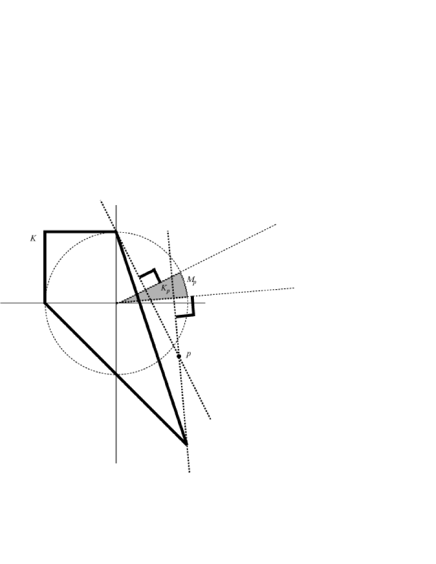
Figure 4.1: The sets $M_{p}$ and $K_{p}$ in $\mathbb{R}^{2}$. Pictured in heavy outline is a set $K$ in $\mathbb{R}^{2}$, where $K:=\mathrm{conv}\{(0,1),(-1,1),(-1,0),(1,-2)\}$. A point $p=(-7/8,-3/4)$ is shown as a heavy dot. The unit circle is drawn in a dashed line. The set $M_{p}$ is the arc of the unit circle that the shaded pie-slice subtends; the set $K_{p}$ is the shaded pie-slice. In two dimensions, the set $M_{p}$ ($K_{p}$) is easy to construct. This construction has been illustrated: draw the two distinct lines through $p$ that are tangent to $K$; the lines that determine the pie-slice are the two straight lines that are perpendicular to the lines through $p$. The idea behind this geometrical construction easily generalises to $\mathbb{R}^{3}$.

The first observation is that, since $K$ properly contains the origin, $M_{p}$ is contained in the hemisphere defined by $\{x:p^{T}x\geq 0\}$:

Fact 13.

For all $m\in M_{p}$, $m^{T}p>0$.

Proof.

Let $m\in M_{p}$. Then $m^{T}p>m^{T}k$ for all $k\in K$. But the fact that the 0-vector is properly contained in $K$ implies that there exists $k\in K$ such that $m^{T}k>0$.∎

The second observation, Lemma 14, is based on the following heuristic, which can be pictured in $\mathbb{R}^{2}$ and $\mathbb{R}^{3}$. Suppose $c$, $||c||=1$, is not in $M_{p}$ (but is reasonably close to $M_{p}$) and that the oracle returns $k_{c}$. What is a natural way to modify the vector $c$, so that it gets closer to $M_{p}$? Intuition dictates moving $c$ away from $k_{c}$ and towards $p$, that is, add a small component of the vector $(p-k_{c})$ to $c$, in order to generate a new guess $c^{\prime}=c+\lambda(p-k_{c})/||p-k_{c}||$, for some $\lambda>0$, which we could then give to the oracle again (see Figure 4.2). Incidentally, I have found that this heuristic actually works: the following little program, in the context of the quantum separability problem, always found entanglement witnesses for entangled states in $\mathbb{H}_{2,2}$, even with very tiny entanglement concurrence [90] (the value of $N^{\prime}$ required depends on the concurrence):

$c:=p/||p||;\hskip 5.69054ptd:=1;\hskip 5.69054pti:=0;$ while  $(d>0$  and  $i<N^{\prime})$  do  $\{$ $k_{c}:=\mathcal{O}_{\text{SOPT}(K)}(c);$ $d:=c^{T}k_{c}-c^{T}p;$ if$\hskip 5.69054pt(d<0)$  then  $\{$ return $c$ $\}$ else  $\{$ $c:=c+d(p-k_{c})/||p-k_{c}||$;  $c:=c/||c||$;  $i:=i+1\}\};$ return “INCONCLUSIVE”

Notice the connection of the above program to the function $d_{\rho}(A)$ of Section 4.2. This program can be regarded as an extremely simple heuristic algorithm for the separation problem when given an optimisation oracle and promised that $p\notin K$ (of course, it may give inconclusive results; in practice, one should set $N^{\prime}$ as large as is practically feasible).

Interestingly, the above heuristic can be formalised as follows. If $c$ is not in $M_{p}$ but is sufficiently close to $M_{p}$, then $c$, $p$, and $k_{c}$ can be used to define a hemisphere which contains $M_{p}$ and whose great circle cuts through $c$. More precisely:

Lemma 14.

Suppose $m\in M_{p}$, $c\notin M_{p}$, and let $\bar{a}:=(p-k_{c})-\mathrm{Proj}_{c}(p-k_{c})$. If $m^{T}c\geq 0$ then $m^{T}\bar{a}>0$.

Proof.

Note that $m^{T}\bar{a}=m^{T}(p-k_{c})-[c^{T}(p-k_{c})](m^{T}c)$. The hypotheses of the lemma immediately imply that $m^{T}(p-k_{c})>0$ and $c^{T}(p-k_{c})\leq 0$. Thus, if $m^{T}c\geq 0$, then $m^{T}\bar{a}>0$. ∎

The lemma gives a method for reducing the search space after each query to $\mathcal{O}_{\text{SOPT}(K)}$ by giving a cutting plane, $\{x:\bar{a}^{T}x=0\}$, that slices off a portion of the search space. The idea is that at each iteration a vector $c\in S_{n}$ is chosen that is approximately in the centre of the remaining search space. Then $c$ is given to the oracle which returns $k_{c}$. If $c^{T}p>c^{T}k_{c}$, then a separating hyperplane for $p$ has been found and the algorithm terminates. Otherwise, as long as $m^{T}c\geq 0$ for all $m\in M_{p}$, the lemma says that the current search space may be sliced through its centre $c$ and the origin, and one half discarded. Because the search space is being approximately halved at each step, the algorithm quickly either finds a separating hyperplane for $p$ or concludes that $p\in K$.

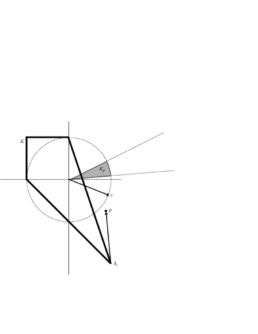
Figure 4.2: Illustration of intuitive heuristic behind Lemma 14. Continuing from Figure 4.1, the unit vector $c$ is a test vector that is close to $M_{p}$ but not in $M_{p}$. Evidently, adding a component of $(p-k_{c})$ to $c$ moves it closer to $M_{p}$.

The above search problem can easily be reduced to an instance of the convex feasibility problem:

Feasibility Problem: Given a convex set $K^{\prime}\subset\mathbf{R}^{n}$, either

1. find a point $k^{\prime}\in K^{\prime}$, or

2. assert that $K^{\prime}$ is empty.

In this case, the convex set $K^{\prime}$ is the set $K_{p}$ which is defined as

$$K_{p}:=\left[\mathrm{ConvexHull}\left(M_{p}\cup\{\bar{0}\}\right)\right]\setminus\{\bar{0}\},$$ (4.2)

where $\bar{0}\in\mathbf{R}^{n}$ denotes the origin. The set $K_{p}$, if not empty, can be viewed as a cone-like object, emanating from the origin and cut off by the unit hypersphere (see Figure 4.1). Several well-known oracle-polynomial-time algorithms exist for the feasibility problem for $K^{\prime}$ in the case where there is a separation oracle for $K^{\prime}$ that, given a test point $y\in\mathbf{R}^{n}$, returns either a hyperplane that separates $y$ from $K^{\prime}$ or asserts that $y\in K^{\prime}$. The oracle $\mathcal{O}_{\text{SOPT}(K)}$, along with Lemma 14, essentially gives a separation oracle for $K_{p}$, as long as the test vectors $c$ given to $\mathcal{O}_{\text{SOPT}(K)}$ satisfy $m^{T}c\geq 0$ for all $m\in M_{p}$. Because of this last requirement, none of the existing algorithms can be applied directly. However, the analytic-center algorithm due to Atkinson and Vaidya [91] beautifully lends itself to a modification that allows the requirement $m^{T}c\geq 0$ for all $m\in M_{p}$ to be satisfied. I will say more about such algorithms in Section 4.6.

Finding a vector in $M_{p}$ and finding a nonzero point in $K_{p}$ are equivalent for our purpose. From now on, we regard the “search space” as the full-dimensional origin-centred hyperball $B_{n}$ in $\mathbf{R}^{n}$; however, to make the analysis more transparent, we will always normalise each test point before giving it to the oracle.

How could we ensure that all our test vectors $c$ satisfy $m^{T}c\geq 0$ for all $m\in M_{p}$? Recall Fact 13, which says that the set $K_{p}$ is contained in the halfspace $\{x:p^{T}x\geq 0\}$. Let $a_{1}:=p/||p||$. Thus, straight away, the search space is reduced to the hemisphere $B_{n}\cap\{x:a_{1}^{T}x\geq 0\}$. The first test vector to give to the oracle $\mathcal{O}_{\text{SOPT}(K)}$ is $p/||p||$, which clearly has nonnegative dot-product with all points in $K_{p}$ and hence all $m\in M_{p}$. By way of induction, assume that, at some later stage in the algorithm, the current search space has been reduced to $P:=B_{n}\bigcap\cap_{i=1}^{h}\{x:a_{i}^{T}x\geq b_{i}\}$ by the generation of cutting planes $\{x:a_{i}^{T}x=b_{i}\}$, where the $a_{i}$, for $i=2,3,\ldots,h$, are the normalised $\bar{a}$ from $h-1$ invocations of Lemma 14. Let $\omega$ be the “centre” of $P$, and suppose that this “centre” is a positive linear combination of the normal vectors $a_{i}$, that is,

$$\omega=\sum_{i=1}^{h}\lambda_{i}a_{i},\hskip 5.69054pt\text{where $\lambda_{i}\geq 0$ for all $i=1,2,\ldots,h$.}$$ (4.3)

Then, by inductive hypothesis, this implies that $m^{T}\omega\geq 0$ for all $m\in M_{p}$. Thus, $c:=\omega/||\omega||$ is a suitable vector to give to the oracle $\mathcal{O}_{\text{SOPT}(K)}$ and use in Lemma 14. Therefore, it suffices to find a definition of “centre $\omega$ of $P$” that satisfies (4.3), in order that all our test vectors $c$ satisfy $m^{T}c\geq 0$ for all $m\in M_{p}$.

Reducing the separation problem for $K$ to the convex feasibility problem for some $K^{\prime}$, while using the optimisation oracle for $K$ as a separation oracle for $K^{\prime}$, is not a new concept in convex analysis. But the precise way that Lemma 14 generates each new cutting plane, incorporating the intuitive correction heuristic, does not appear in the literature. This is likely because there is a well-known, standard way to carry out such a reduction, which I cover in the next section.

4.5 Connection to standard method

The standard way to perform the reduction of the last section may be found in the synthesis of Lemma 4.4.2 and Theorem 4.2.2 in [1].

Definition 21 (Polar of $K$).

The polar $K^{\star}$ of a full-dimensional convex set $K\subset\mathbb{R}^{n}$ that contains the origin is defined as

$$K^{\star}:=\{c\in\mathbb{R}^{n}:c^{T}x\leq 1\hskip 5.69054pt\forall x\in K\}.$$ (4.4)

If $c\in K^{\star}$, then the plane $\pi_{c,1}\equiv\{x:c^{T}x=1\}$ separates $p\in\mathbb{R}^{n}$ from $K$ when $c^{T}p>1$. Thus, the separation problem for $p$ is equivalent to the feasibility problem for $Q_{p}$, defined as

$$Q_{p}:=K^{\star}\cap\{c:p^{T}c\geq 1\}.$$ (4.5)

As mentioned in the previous section (and elaborated on in the next section), to solve the feasibility problem for any $K^{\prime}$, it suffices to have a separation routine for $K^{\prime}$. Because we can easily build a separation routine $\mathcal{O}_{\text{SSEP}(Q_{p})}$ for $Q_{p}$ out of $\mathcal{O}_{\text{SSEP}(K^{\star})}$, it suffices to have a separation routine $\mathcal{O}_{\text{SSEP}(K^{\star})}$ for $K^{\star}$ in order to solve the feasibility problem for $Q_{p}$. Building $\mathcal{O}_{\text{SSEP}(Q_{p})}$ out of $\mathcal{O}_{\text{SSEP}(K^{\star})}$ is done as follows:

Routine $\mathcal{O}_{\text{SSEP}(Q_{p})}(y)$:
case: $p^{T}y<1$
return $-p$
else: $p^{T}y\geq 1$
call $\mathcal{O}_{\text{SSEP}(K^{\star})}(y)$
case: $\mathcal{O}_{\text{SSEP}(K^{\star})}(y)$ returns separating vector $q$
return $q$
else: $\mathcal{O}_{\text{SSEP}(K^{\star})}(y)$ asserts $y\in K^{\star}$
return “$y\in Q$”

It remains to show that the optimisation routine $\mathcal{O}_{\text{SOPT}(K)}$ for $K$ gives a separation routine $\mathcal{O}_{\text{SSEP}(K^{\star})}$ for $K^{\star}$. Suppose $y$ is given to $\mathcal{O}_{\text{SOPT}(K)}$, which returns $k\in K$ such that $y^{T}x\leq y^{T}k=:b$ for all $x\in K$. If $b\leq 1$, then $\mathcal{O}_{\text{SSEP}(K^{\star})}$ may assert $y\in K^{\star}$. Otherwise, $\mathcal{O}_{\text{SSEP}(K^{\star})}$ may return $k$, because $\pi_{k,1}$ (and hence $\pi_{k,b}$) separates $y$ from $K^{\star}$: since $k^{T}y=b>1$, it suffices to note that $k^{T}c=c^{T}k\leq 1$ for all $c\in K^{\star}$ by the definition of $K^{\star}$ and the fact that $k\in K$.

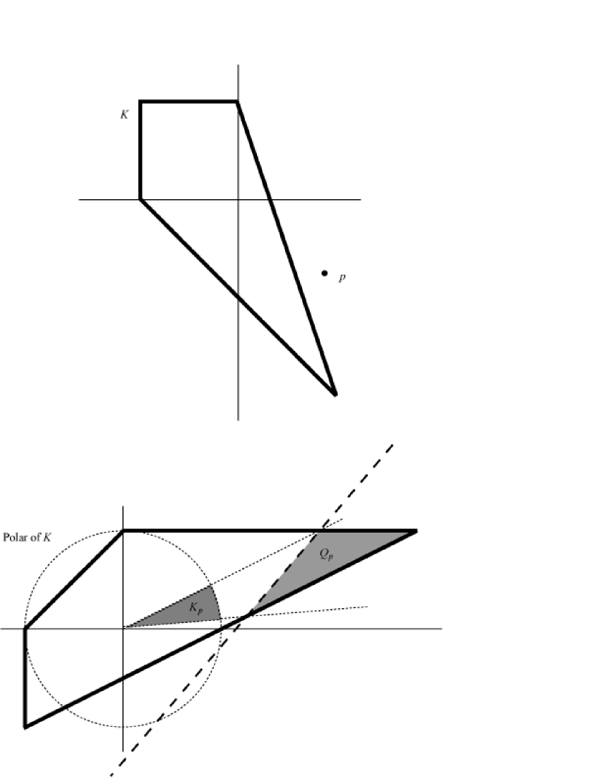
Figure 4.3: The upper picture is a set $K$ in $\mathbb{R}^{2}$, where $K:=\mathrm{conv}\{(0,1),(-1,1),(-1,0),(1,-2)\}$. A point $p=(-7/8,-3/4)$ is shown. The polar $K^{\star}$ of $K$ is shown in heavy outline in the lower picture; $K^{\star}=\mathrm{conv}\{(0,1),(-1,0),(-1,-1),(3,1)\}$. The set $Q_{p}$ is the shaded polytope, bounded by the long-dashed plane $\{c:p^{T}c=1\}$. The set $K_{p}$ is the shaded pie-slice and is the radial projection of $Q_{p}$ onto the origin-centred unit ball (whose boundary is shown as a short-dashed circle). The particular $K$ and $K^{\star}$ are taken from [44].

Figure 4.3 shows the relationship between the method of Section 4.4 and the above method, by illustrating that the set $K_{p}$ (defined in (4.2)) is just the radial projection of $Q_{p}$ onto $B_{n}$. Thus, unsurprisingly, both methods test the feasibility of virtually the same thing. The novelty of the method of Section 4.4 lies in the way the cutting planes are generated.

4.6 Cutting-plane algorithms for convex feasibility for $K^{\prime}$

Some remarks about convex feasibility cutting-plane algorithms for $K^{\prime}\subset\mathbb{R}^{n}$, relative to a separation oracle $\mathcal{O}_{\text{SSEP}(K^{\prime})}$, are in order. All such algorithms have the same basic structure:

1. Define a (possibly very large) regular bounded convex set $P_{0}$ which is guaranteed to contain $K^{\prime}$, such that, for some reasonable definition of “centre”, the centre $\omega_{0}$ of $P_{0}$ is easily computed. The set $P_{0}$ is called an outer approximation to $K^{\prime}$. Common choices for $P_{0}$ are the origin-centred hyperbox, $\{x\in\mathbb{R}^{n}:-2^{L}\leq x_{i}\leq 2^{L},\hskip 5.69054pt1\leq i\leq n\}$ and the origin-centred hyperball, $\{x:x^{T}x\leq 2^{L}\}$ (where $2^{L}$ is a trivially large bound).

2. Give the centre $\omega$ of the current outer approximation $P$ to $\mathcal{O}_{\text{SSEP}(K^{\prime})}$.

3. If $\mathcal{O}_{\text{SSEP}(K^{\prime})}$ asserts “$\omega\in K^{\prime}$”, then HALT.

4. Otherwise, say $\mathcal{O}_{\text{SSEP}(K^{\prime})}$ returns the hyperplane $\pi_{c,b}$ such that $K^{\prime}\subset\{x:c^{T}x\leq b\}$. Update (shrink) the outer approximation $P:=P\cap\{x:c^{T}x\leq b^{\prime}\}$ for some $b^{\prime}\geq b$. Possibly perform other computations to further update $P$. Check stopping conditions; if they are met, then HALT. Otherwise, go to step (ii).

The difficulty with such algorithms is knowing when to halt in step (iv). Generally, the stopping conditions are related to the size of the current outer approximation. Because it is always an approximate (weak) feasibility problem that is solved, the associated accuracy parameter $\delta$ can be exploited to get a “lower bound” $V$ on the “size” of $K^{\prime}$, with the understanding that if $K^{\prime}$ is smaller than this bound, then the algorithm can correctly assert that $S(K^{\prime},-\delta)$ is empty. Thus the algorithm stops in step (iv) when the current outer approximation is smaller than $V$.

The cutting-plane algorithm is called (oracle-) polynomial-time if it runs in time
$O(\text{poly}(n,\log(1/\delta)))$ with unit cost for the oracle. It is called (oracle-) fully polynomial if it runs in time $O(\text{poly}(n,1/\delta))$. This thesis is concerned primarily with polynomial-time cutting-plane algorithms.

Using the standard cut-generation rule, there are a number of polynomial-time convex feasibility algorithms that can be applied (see [91] for a discussion of all of them). The three most important are the ellipsoid method, the volumetric centre method, and the analytic centre method. The ellipsoid method has $P_{0}=\{x:x^{T}x\leq 2^{L}\}$ and is the only one which requires “further update” of the outer approximation $P$ in step (iv) after a cut has been made – a new minimal-volume ellipse is drawn around $P:=P\cap\{x:c^{T}x\leq b^{\prime}\}$. The ellipsoid method, unfortunately, suffers badly from gigantic precision requirements, making it unusable in practice. The volumetric centre and analytic centre algorithms are more efficient than the ellipsoid algorithm and are very similar to each other in complexity and precision requirements, with the analytic centre algorithm having some supposed practical advantages.

The cutting plane $\{x:c^{T}x=b^{\prime}\}$ requires further definition:

$$\text{If }\left\{\begin{array}[]{rcl}b^{\prime}&<&c^{T}\omega\\ b^{\prime}&=&c^{T}\omega\\ b^{\prime}&>&c^{T}\omega\end{array}\right\}\text{ then the above is a }\left\{\begin{array}[]{c}\text{\emph{deep-cut}}\\ \text{\emph{central-cut}}\\ \text{\emph{shallow-cut}}\end{array}\right\}\text{ algorithm.}$$ (4.6)

Intuitively, deep-cut algorithms should be fastest. Ironically, though, except for the case of ellipsoidal algorithms (which are practically inefficient), the algorithms that are provably polynomial-time are central- or even shallow-cut algorithms. For instance, even though $\mathcal{O}_{\text{SSEP}(K^{\star})}$, built on $\mathcal{O}_{\text{SOPT}(K)}$, gives deep cuts $\pi_{k,1}$, it is not known how to utilise the deep cuts to get a polynomial-time algorithm using analytic or volumetric centers. Note that the new cut-generation method in Section 4.4 is capable only of giving central cuts; but this does not, a priori, put it at any disadvantage (relative to the standard cut-generation method) with regard to polynomial-time analytic or volumetric centre algorithms. We will see in Chapter 5 that this new cut-generation rule indeed yields a polynomial-time algorithm.

4.7 A new quantum separability algorithm

The algorithm in Chapter 5, which is based on analytic centres, gives a new method for solving the quantum separability problem by solving $\text{WSEP}_{\text{In}}(\mathcal{S}_{M,N})$. As we will see, the number of arithmetic operations required by the algorithm is

$$O((T+M^{6}N^{6}\log(1/\delta))M^{2}N^{2}\log^{2}(M^{2}N^{2}/\delta)),$$ (4.7)

where $T$ is the cost of one call to the WOPT($\mathcal{S}_{M,N}$) routine.

Now consider the complexity of computing an instance $(A,\epsilon)$ of WOPT($\mathcal{S}_{M,N}$). The only way to get an upper bound on this complexity is to assume the most naive way to carry out this computation, which is to one-by-one calculate $\textrm{tr}(A\sigma)$ for each of the pure separable states $\sigma$ to a sufficiently high precision, and then return the $\sigma$ that produced the largest value of $\textrm{tr}(A\sigma)$.

I use the same framework and notation of Section 3.3.1. Suppose $\sigma=\alpha\alpha^{\dagger}\otimes\beta\beta^{\dagger}$ maximises $\textrm{tr}(A\sigma)$, and, as before, let $\tilde{\alpha}$ and $\tilde{\beta}$ be the $p^{\prime}$-bit truncations of $\alpha$ and $\beta$. Let $\gamma:=\alpha\alpha^{\dagger}\otimes\beta\beta^{\dagger}-\tilde{\alpha}\tilde{\alpha}^{\dagger}\otimes\tilde{\beta}\tilde{\beta}^{\dagger}$. The real coordinates of the entries of $[\gamma]$ have absolute value no greater than $2^{-(p^{\prime}-6)}$. Since we give to the WOPT($\mathcal{S}_{M,N}$) routine an $A$ such that $||A||_{2}=1$, we have $||A||_{1}\leq\sqrt{MN}||A||_{2}=\sqrt{MN}$ which, since $A$ is normal, is equivalent to $\sum_{ij}|A_{ij}|\leq\sqrt{MN}$ [92], where $A_{ij}$ are the entries of $[A]$. This gives a bound of $|A_{ij}|\leq\sqrt{MN}$. It follows that

$$\textrm{tr}(A(\alpha\alpha^{\dagger}\otimes\beta\beta^{\dagger}))-\textrm{tr}(A(\tilde{\alpha}\tilde{\alpha}^{\dagger}\otimes\tilde{\beta}\tilde{\beta}^{\dagger})) = \textrm{tr}(A\gamma)$$ (4.8)

$$\leq M^{2.5}N^{2.5}2^{-(p^{\prime}-7)}.$$ (4.9)

We set $p^{\prime}$ such that $M^{2.5}N^{2.5}2^{-(p^{\prime}-7)}<\epsilon$, which gives

$$p^{\prime}>\log_{2}\left(\frac{M^{2.5}N^{2.5}}{\epsilon}\right)+7.$$ (4.10)

This gives

$$T \backsim \Omega_{p^{\prime}}\text{poly}(M,N,1/\delta)$$ (4.11)

$$\lesssim \left(\frac{2^{7}M^{2.5}N^{2.5}}{\epsilon}\right)^{2(M+N)}\text{poly}(M,N,1/\delta).$$ (4.12)

In practice, however, it need not be so bad. We can formulate the optimisation problem as the (constrained or unconstrained) maximisation of a real function $f(\sigma):=\textrm{tr}(A\sigma)$ of real variables parametrising $\sigma$, and then apply continuous optimization methods to $f$. Denote by $f^{*}$ the global maximum of $f$. As the global optimisation algorithm proceeds, it may give progressively better lower and upper bounds on $f^{*}$. Call these bounds $\underline{f}$ and $\overline{f}$, respectively. A key advantage of the algorithm is that, during any computation of $\mathcal{O}(A)$, the search for $f^{*}$ may be halted early when either (i) $\textrm{tr}(A\rho)\leq\underline{f}$, in which case Lemma 14 can be invoked to generate a new cutting plane, or (ii) $\overline{f}<\textrm{tr}(A\rho)$, in which case the algorithm has found an entanglement witness for $\rho$. Note that lower bounds $\underline{f}$ can be generated very quickly using local optimisation routines seeded at random points in the domain of $f$. Thus, the algorithm’s run time may be significantly shorter than the worst-case complexity of WOPT($\mathcal{S}_{M,N}$) predicts.

4.8 Complexity comparison of algorithms

All of the algorithms considered solve the weak membership problem for $\mathcal{S}_{M,N}$ with accuracy parameter $\delta$. How does the new separability algorithm of the previous section compare to the others?

Recall the reasonable presumption that the numerical integration in Zapatrin’s algorithm (Section 3.3.4) is far more computationally intensive than the global minimisation of the new algorithm. Recall also that Pérez-Garcia’s algorithm (Section 3.3.3) is not clearly related to the weak membership problem, barring new results about the $||\cdot||_{\gamma}$-norm and robustness of entanglement.

The following table summarises the dominating factors (that are at least factorial in $M$ or $N$) in the run-times of the new algorithm and the algorithms of Sections 3.3.1 and 3.3.2:

Search for separable decomposition (Section 3.3.1)	$(MN/\delta)^{O(M^{3}N^{2}+M^{2}N^{3})}$
Bounded search for symmetric extensions (Section 3.3.2)	$(M/\delta)^{O(M)}$
Search for entanglement witness (Section 4.7)	$(MN/\delta)^{O(M+N)}$

Of the three algorithms in the table, the search for separable decompositions is, as expected, the most complex.

A few remarks are in order regarding the new algorithm and the bounded search for symmetric extensions. Right away, we can see that if $M$ is a constant, then the bounded search for symmetric extensions has a much lower complexity. Note, however, that if $M=N$, then the two complexities, as summarised in the table, become the same. As a related side point, note that Gurvits [67] has actually shown WMEM$(\mathcal{S}_{M,N})_{M,N}$ to be NP-hard when $M\leq N\leq M(M-1)/2$; it is an open problem as to whether, say, WMEM$(\mathcal{S}_{2,N})_{N}$ is NP-hard. So, if we want to be absolutely sure we are solving a hard problem, we can restrict to the case where $M=N$. In this case, it is easy to check that the detailed complexity estimates given previously indicate that the new algorithm has a better complexity, even when we take into account that the bounded search for symmetric extensions uses the trace norm as opposed to the Euclidean norm. Recall that the bounded search for symmetric extensions has complexity on the order of $d^{4}_{S_{k}}$, where we can invoke the lower bound $d_{S_{\bar{k}}}>\left({16M^{11}}/{\delta^{2}}\right)^{M-1}$ from equation (3.45) to get $d^{4}_{S_{k}}>2^{16M-4}M^{44M}/\delta^{8M-8}$. But the algorithm gets a complexity reduction for solving the weak membership problem with respect to the trace distance instead of the Euclidean distance. This reduction corresponds to substituting $M\delta$ for $\delta$ in the above lower bound, which gives the best known lower bound on the complexity of the bounded search for symmetric extensions of

$$2^{16M-4}M^{36M+8}\left(\frac{1}{\delta}\right)^{8M-8}.$$ (4.13)

The dominant factor in the run-time estimate of the new algorithm, which appears in (4.12), is $\left({2^{7}M^{2.5}N^{2.5}}/{\epsilon}\right)^{2(M+N)}$. In Chapter 5, we will see that $\epsilon:=\delta/5$. Making this substitution and setting $N:=M$ gives an upper bound (ignoring polynomial factors) on the run time of the new algorithm of

$$2^{40M}M^{20M}\left(\frac{1}{\delta}\right)^{4M}.$$ (4.14)

The factors in (4.13) and (4.14) that are at least factorial in $M$ are, respectively, $M^{36M+8}$ and $M^{20M}$, the former being larger. As well, the dependence on $\delta$ in (4.13) is worse than that in (4.14). Therefore, the new algorithm has the smaller run-time estimate when $M=N$.

Chapter 5 New polynomial-time reduction from WSEP to WOPT

As promised, I now show that the cut-generation rule of Section 4.4, which is based on an intuitive heuristic, yields an oracle-polynomial-time algorithm for the in-biased weak separation problem for a convex set $K\subset\mathbb{R}^{n}$ relative to an oracle for the weak optimization problem for $K$; we only assume that $K$ contains a ball of finite radius centered at a known point $c_{0}$ and is contained in a ball of finite radius $R$. The algorithm uses $O(\text{poly}(n,\log(R/\delta)))$ calls to the weak optimisation oracle, where $\delta$ is the accuracy parameter that appears in Definition 19. For the remainder of this thesis, $\mathcal{O}$ will denote the oracle for the weak optimisation problem for $K$. One simplifying assumption that we will carry through this chapter, without loss of generality, is that $c_{0}$ is the origin. This new algorithm is based on the analytic centre cutting-plane algorithm of Atkinson and Vaidya [91].

Continuing the discussion in the previous chapter, Section 5.1 gives the main idea behind the new algorithm. Section 5.2 presents the algorithm in terms of parameters that will be given in section 5.3, which contains the proof of correctness of the algorithm. Section 5.4 discusses complexity and relates the algorithm to the standard cut-generation method of Section 4.5. Section 5.5 gives the algorithm’s parameters for the specific case of the quantum separability problem.

5.1 The Main Idea of the Algorithm

The general idea of the algorithm is as follows. Let $P$ be the current outer approximation $P:=B_{n}\bigcap\cap_{i=1}^{h}\{x:a_{i}^{T}x\geq b_{i}\}$, as described in the second-last paragraph of Section 4.4. Recall that we need a definition of “centre $\omega$ of $P$” that satisfies (4.3). Define the analytic centre $\omega$ of $P$ as the unique minimiser of the real convex function

$$F(x):=-\sum_{i=1}^{h}\log(a_{i}^{T}x-b_{i})-\log(1-x^{T}x).$$ (5.1)

The relation $\nabla F(\omega)=0$ gives

$$\omega=\frac{1-\omega^{T}\omega}{2}\sum_{i=1}^{h}\frac{a_{i}}{a_{i}^{T}\omega-b_{i}},$$ (5.2)

which shows that $\omega$, defined as the analytic centre of $P$, indeed satisfies (4.3).

The algorithm stops when the current outer approximation becomes either too small (volume-wise) or too thin to contain $K_{p}$. For this, a lower bound $r>0$ on the radius of the largest ball contained in $K_{p}$ is needed. By exploiting the accuracy parameter $\delta$ of the weak separability problem, such an $r$ exists and is derived in section 5.3.3.

The actual algorithm is not as straightforward. For instance, each time a new cutting plane is added, it is shifted by some amount ($b_{i}<0$) so as to keep the analytic centre of the old $P$ in the new $P$. As well, cutting planes are occasionally discarded so that $h$ does not exceed some prespecified number. This shifting and discarding of hyperplanes is done exactly as in [91]. To facilitate comparison, we use notation that corresponds to the notation used in [91].

5.2 The Algorithm

Following [91], the algorithm utilises three types of quantities ($\sigma_{i}(z)$, $\kappa(a_{i},b_{i})$, and $\mu_{i}(z)$), whose significance we now briefly explain. Suppose that $P=B_{n}\bigcap\cap_{i=1}^{h}\{x:a_{i}^{T}x\geq b_{i}\}$ is the current search space at some stage during the algorithm; that is, suppose a total of $h$ cutting planes have been generated. Denote the hyperplane $\{x:a^{T}_{i}x-b_{i}=0\}$ by the ordered pair $(a_{i},b_{i})$. Recall that for any positive definite matrix $A$, one can define the ellipsoid $E(A,z,r)$ as

$$E(A,z,r):=\{x\in\mathbf{R}^{n}:(x-z)^{T}A(x-z)\leq r^{2}\}.$$ (5.3)

When $A=\nabla^{2}F(z)$, we refer to $E(A,z,r)$ as the Hessian ellipsoid.

We mentioned that one of the stopping conditions is that the volume of $P$ gets too small to contain $K_{p}$. Later we will see that the volume of $P$ can be related to the determinant of $\nabla^{2}F(\omega)$, where $\omega$ is the analytic center of $P$. Define the quantities

$$\sigma_{i}(x):=\frac{a_{i}^{T}(\nabla^{2}F(x))^{-1}a_{i}}{(a_{i}^{T}x-b_{i})^{2}},\hskip 5.69054pt1\leq i\leq h$$ (5.4)

for $x\in P$. The denominator is the square of the distance from $x$ to the hyperplane $(a_{i},b_{i})$. The numerator is the square of the radius of the Hessian ellipsoid $E(\nabla^{2}F(x),x,1)$ in the direction of $a_{i}$. In Lemma 17, we will see that $E(\nabla^{2}F(x),x,1)\subset P$. The smaller the quantity $\sigma_{i}(x)$, the further away the hyperplane $(a_{i},b_{i})$ is from the ellipsoid $E(\nabla^{2}F(x),x,1)$. If $z$ is an approximate analytic center of $P$, then a sufficiently small value of $\sigma_{i}(z)$ will indicate that $(a_{i},b_{i})$ has a small effect on $\det(\nabla^{2}F(z))$ and so it can be discarded because it does not sufficiently affect the volume of $P$.

Computing $\sigma_{i}(z)$ values is relatively computationally expensive, so there is a simple test that can trigger a check of $\sigma_{i}(z)$. When the hyperplane $(a_{i},b_{i})$ is first introduced, the quantity $\kappa(a_{i},b_{i})$ is set to $a_{i}^{T}z-b_{i}$, which is the distance from $(a_{i},b_{i})$ to the approximate analytic center $z$ of $P$. If, at some later step, we find that the distance from the current approximate analytic center $z$ to $(a_{i},b_{i})$ has doubled, then the quantity $\sigma_{i}(z)$ is computed and tested. We denote the ratio of the current distance to the original distance by $\mu_{i}(z):=(a_{i}^{T}z-b_{i})/\kappa(a_{i},b_{i})$. If $\sigma_{i}(z)$ is not sufficiently small, then $\kappa(a_{i},b_{i})$ is reset to the current distance.

To compute approximate analytic centers, we use the Newton method. A useful function that measures the quality of the approximation is

$$\lambda(x):=\sqrt{\nabla F(x)^{T}(\nabla^{2}F(x))^{-1}\nabla F(x)}.$$ (5.5)

As well, define the function $q_{\lambda}:=1-(1-3\lambda)^{1/3}$ for $\lambda\in\mathbf{R}$, and the function $\Psi(x):=(\lambda(x))^{2}$.

The subscripts ‘d’ and ‘a’ in the algorithm mean ‘after a hyperplane is discarded’ or ‘after a hyperplane is added’, respectively.

The algorithm is presented in terms of undefined constants (all variables with the subscript “$0$”, plus $\nu$) and parameters ($r$,$u$,$\tilde{\delta}$). For a list of the definitions of the parameters and suitable values of the constants, the reader may consult subsection 5.3.5.

The stopping conditions in the following algorithm are required for the proof of polynomial-time convergence, but they are not the best conditions to use in practice. In subsection 5.3.6, we give tighter stopping conditions that depend more heavily on $z$ and $\nabla^{2}F(z)$.

The algorithm for the in-biased weak separation problem for $K$, relative to an oracle for the weak optimization problem for $K$, is as follows:

begin
initialise$\{$
$a_{1}:=p/||p||$
$P:=B_{n}\cap\{x:a_{1}^{T}x\geq 0\}$
$z:=a_{1}/\sqrt{3}$
$\kappa(a_{1},b_{1}):=1/\sqrt{3}\}$
do$\{$
if $\max_{i}\mu_{i}(z)>2$ then
Case 1:
if there is an index $j$ such that $\mu_{j}(z)>2$ and $\sigma_{j}(z)<\sigma_{0}$ then
Subcase 1.1:
Discard $(a_{j},b_{j})$ from the set of hyperplanes defining $P$, yielding a new
region $P_{\mathrm{d}}$; $P_{\mathrm{new}}:=P_{\mathrm{d}}$.
Starting at $x_{0}:=z$, iterate Newton steps $x_{i}$ until both
$\lambda(x_{i})<\rho_{0}$ and $q_{\lambda(x_{i})}<\frac{\tilde{\delta}}{1+\tilde{\delta}}\frac{||x_{i}||}{\sqrt{2}}$ to get a new approximation $z_{\mathrm{d}}:=x_{i}$
to the new analytic center $\omega_{\mathrm{d}}$ of $P_{\mathrm{d}}$; $z_{\mathrm{new}}:=z_{\mathrm{d}}$.
else
Subcase 1.2:
Let $(a_{j},b_{j})$ be any hyperplane such that $\mu_{j}(z)>2$.
Reset $\kappa(a_{j},b_{j}):=a_{j}^{T}z-b_{j}$.
endif
else
Case 2:
Call weak optimization oracle on $c:=z/||z||$ with $\epsilon:=\delta/5$.
if oracle outputs $k_{c}\in K$ such that $c^{T}p\geq c^{T}k_{c}+\delta/5$ then
return $c$.
endif
$a:=(p-k_{c})-c^{T}(p-k_{c})c$; $a:=a/||a||$.
Compute $\beta<0$ such that $\gamma^{2}:=(a^{T}[\nabla^{2}F(z)]^{-1}a)/(a^{T}z-\beta)^{2}=\gamma_{0}^{2}$.
Add $(a,\beta)$ to the set of hyperplanes defining $P$, that is,
set $P_{\mathrm{a}}:=P\cap\{x:a^{T}x\geq\beta\}$; $P_{\mathrm{new}}:=P_{\mathrm{a}}$.
Starting at $x_{0}:=z$, iterate Newton steps $x_{i}$ until both
$\lambda(x_{i})<\rho_{0}$ and $q_{\lambda(x_{i})}<\frac{\tilde{\delta}}{1+\tilde{\delta}}\frac{||x_{i}||}{\sqrt{2}}$ to get a new approximation $z_{\mathrm{a}}:=x_{i}$
to the new analytic center $\omega_{\mathrm{a}}$ of $P_{\mathrm{a}}$; $z_{\mathrm{new}}:=z_{\mathrm{a}}$.
Set $\kappa(a,\beta):=a^{T}z_{\mathrm{a}}-\beta$.
endif
$P:=P_{\mathrm{new}}$; $z:=z_{\mathrm{new}}$.$\}$
until$\{$
Stopping Condition 1: $h\geq\nu nu(n,\delta)$, or
Stopping Condition 2: $2r>\frac{[\min_{i}\{a_{i}^{T}z-b_{i}\}]}{1-\zeta_{0}}(3h+4)$$\}$
enddo
return “$p\in S(K,\delta)$”
end

5.3 Proof of Correctness of the Algorithm

To prove that the algorithm is correct, we need to deal with the fact that the algorithm is run on a computer with fixed precision. If the volume and width of $K_{p}$ are to be lower-bounded, then clearly we need to exploit the weakness of the separability problem; that is, we only need to find a separating hyperplane for $p$ when $p$ is outside of $S(K,\delta)$. This would give a lower bound on the volume and width of $K_{p}$ in terms of $n$, $R$, and $\delta$. We present the convergence proofs next, assuming that we have a lower bound $r$ on the maximum radius of a ball contained in $K_{p}$:

$$r<\sup_{x}\{r^{\prime}\in\mathbf{R^{+}}:B(x,r^{\prime})\subset K_{p}\},$$ (5.6)

where $B(x,r):=\{y\in\mathbf{R}^{n}:||y-x||\leq r\}$ and $\mathbf{R}^{+}$ denotes the positive real numbers. In subsection 5.3.2, we will derive a suitable $r=r(n,R,\delta)$. The volume of a hypersphere of radius $r$ in $\mathbf{R}^{n}$ is lower-bounded by $(r/n)^{n}$ [1]. Thus, inequality (5.6) gives

$$\textrm{volume($K_{p}$)}\geq\left(\frac{r}{n}\right)^{n}.$$ (5.7)

We note here expressions for the gradient $\nabla F(x)$ and Hessian $\nabla^{2}F(x)$ of the function $F(x)$ as defined in (5.1):

$$\nabla F(x) = -\sum_{i=1}^{h}\frac{a_{i}}{a_{i}^{T}x-b_{i}}+\frac{2x}{1-x^{T}x}$$

$$\nabla^{2}F(x) = \sum_{i=1}^{h}\frac{a_{i}a_{i}^{T}}{(a_{i}^{T}x-b_{i})^{2}}+\frac{4xx^{T}}{(1-x^{T}x)^{2}}+\frac{2I}{1-x^{T}x},$$

where $I$ denotes the identity operator.

The full proof will be given in stages. In subsection 5.3.1, we will present the results required to prove that the algorithm works with the assumptions that the cutting planes generated do not cut into the set $K_{p}$ and that sufficiently good approximations of the analytic centers are at hand. The proofs (mostly appearing in the Appendix) will be left in terms of parameters including various constants and the inner radius $r$. In subsection 5.3.2, we show that such correct cutting planes can be generated. In subsection 5.3.3, we derive a suitable value for $r$. In subsection 5.3.4, we describe the Newton method used to calculate approximate analytic centers and show that the number of required Newton iterations is small. In subsection 5.3.5, we give concrete values for all constants.

Before diving into the tough stuff, I show that the initialisation of the analytic centre $z:=a_{1}/\sqrt{3}$ is correct. I actually prove something slightly more general, which will come up in the discussion in Section 5.4.

Fact 15.

For $||a_{1}||=1$, the analytic centre $\omega$ of $\{x:x^{T}x\leq R^{\star}\}\cap\{x:a_{1}^{T}x-s\geq 0\}$, for $s\geq 0$, is

$$\omega=\frac{s+\sqrt{s^{2}+3R^{\star}}}{3}a_{1}.$$ (5.8)

Proof.

The equation $\nabla F(\omega)=0$ (for the barrier of radius $R^{\star}$) gives

$$\frac{2\omega}{R^{\star}-\omega^{T}\omega}=\frac{a_{1}}{a_{1}^{T}\omega-s}.$$ (5.9)

This implies that $\omega=\lambda a_{1}$ for some $\lambda>0$. Making this substitution and solving for $\lambda$ gives $3\lambda^{2}-2s\lambda-R^{\star}=0$, which gives the required result. ∎

5.3.1 Convergence

The new algorithm for the feasibility problem for $K_{p}$ differs from the one in [91] in two essential ways:

1. I do not assume that we have an unrestricted, unweakened separation oracle for $K_{p}$. Rather, we assume that we have a weakened separation oracle (built from the weak optimization oracle for $K$ and Lemma 14) which is restricted in that it can only handle queries $c$ satisfying $m^{T}c\geq 0$ for all $m\in K_{p}$.

2. To accommodate the above restriction, I use the $\bar{0}$-centered unit hyperball $B_{n}$ containing $K_{p}$ as the initial search space instead of a $\bar{0}$-centered hyperbox $\{x\in\mathbf{R}^{n}:-2^{L}\leq x_{i}\leq 2^{L},1\leq i\leq n\}$.

The second item above means that the current search space $P$ is never a polytope. Consequently, most of the lemmas of [91] that are properties of the function $F(x)$ cannot be used without modification. Luckily, though, the function $F(x)$ is a self-concordant functional [94] which has all the analogous properties necessary to make the proofs of [91] work for our algorithm. I present these fundamental lemmas below; the corresponding label number in [91] will appear in parentheses after our label number. In the following, assume $P=B_{n}\bigcap\cap_{i=1}^{h}\{x:a_{i}^{T}x\geq b_{i}\}$ and $F(x):=-\sum_{i=1}^{h}\log(a_{i}^{T}x-b_{i})-\log(1-x^{T}x)$ for $h\geq 0$, so that the interior of $P$ is the domain of $F$. As always, $\omega$ denotes the analytic center (unique minimiser) of $P$ ($F(x)$).

Lemma 16 (Line (2) in [91]).

Let $A$ be positive definite. For any fixed vector $w$ in $\mathbf{R}^{n}$,

$$\max_{x\in E(A,z,r)}w^{T}(x-z)=r\sqrt{w^{T}A^{-1}w}.$$

Proof.

See [1], for example. ∎

Lemma 17 (Lemma 1 in [91]).

For every $z\in P$, $E(\nabla^{2}F(z),z,1)\subset P$.

Proof.

Follows from definition of self-concordance; see [94] or [95]. ∎

Lemma 18 (Lemma 3 in [91]).

If $\alpha<1$ and $y\in E(\nabla^{2}F(z),z,\alpha)$, then

$$(1-\alpha)^{2}\xi^{T}\nabla^{2}F(z)\xi\leq\xi^{T}\nabla^{2}F(y)\xi\leq(1-\alpha)^{-2}\xi^{T}\nabla^{2}F(z)\xi$$ (5.10)

for all $\xi\in\mathbf{R}^{n}$.

Proof.

Follows from definition of self-concordance; see [94] or [95]. ∎

Lemma 19 (Corollary 4 in [91]).

Suppose $A$ and $B$ are positive definite $n\times n$ matrices such that $\xi^{T}A\xi\geq\theta\xi^{T}B\xi$ for some $\theta>0$ and for all $\xi\in\mathbf{R}^{n}$. Then $\xi^{T}A^{-1}\xi\leq\theta^{-1}\xi^{T}B^{-1}\xi$ for all $\xi\in\mathbf{R}^{n}$.

Proof.

See proof of Lemma 2 in [96]. ∎

Recall the second-degree Taylor expansion of $F(y)$ about $z\in\mathbf{R}^{n}$:

$$F(y)-F(z)=\nabla F(z)^{T}(y-z)+\frac{1}{2}(y-z)^{T}\nabla^{2}F(z)(y-z)+\mathrm{Error}.$$ (5.11)

Lemma 20 (Lemma 5 in [91]).

If $y\in E(\nabla^{2}F(z),z,\alpha)$ where $\alpha<1$, then the error in using the second-degree Taylor polynomial constructed about $z$ to approximate $F(y)$ satisfies $|\mathrm{Error}|\leq\frac{\alpha^{3}}{3(1-\alpha)}$.

Proof.

See proof of Theorem 2.2.2 in [94]. ∎

Lemma 21 (Lemma 6 in [91]).

If $\lambda(z)<\frac{1}{3}$, then $F(z)-F(\omega)\leq\frac{1}{2}q^{2}_{\lambda(z)}\frac{1+q_{\lambda(z)}}{1-q_{\lambda(z)}}$.

Proof.

See proof of Theorem 2.2.2 (iii) (line 2.2.15) in [95]. ∎

Lemma 22 (Lemma 7 in [91]).

Let $\alpha:=\sqrt{(\omega-z)^{T}\nabla^{2}F(z)(\omega-z)}$. If $\lambda(z)<\frac{1}{3}$, then $\alpha\leq q_{\lambda(z)}$.

Proof.

See proof of Theorem 2.2.2 (iii) (line 2.2.17) in [95]. ∎

The next lemma gives a Hessian ellipsoid centered at the analytic center $\omega$ which contains the current search space $P$. The volume of the ellipsoid gives an upper bound on the volume of $P$ which is useful for knowing when $P$ is too small to contain $K_{p}$.

Lemma 23 (Lemma 9 in [91]).

If $h>31$ then $P\subset E(\nabla^{2}F(\omega),\omega,\sqrt{14}h)$.

Proof.

Since $\omega$ is the unique minimiser of $F(x)$, we have

$$\bar{0}^{T}=(\nabla F(\omega))^{T}=\sum_{i=1}^{h}\frac{-a^{T}_{i}}{a_{i}^{T}\omega-b_{i}}+\frac{2\omega^{T}}{1-\omega^{T}\omega}\Leftrightarrow\frac{2\omega^{T}}{1-\omega^{T}\omega}=\sum_{i=1}^{h}\frac{a_{i}^{T}}{a_{i}^{T}-b_{i}}.$$

Therefore,

$$h = \sum_{i=1}^{h}\frac{a_{i}^{T}\omega-b_{i}}{a_{i}^{T}\omega-b_{i}}=\left(\sum_{i=1}^{h}\frac{a_{i}^{T}}{a_{i}^{T}\omega-b_{i}}\right)(\omega)-\sum_{i=1}^{h}\frac{b_{i}}{a_{i}^{T}\omega-b_{i}}$$

$$= \frac{2\omega^{T}\omega}{1-\omega^{T}\omega}+\sum_{i=1}^{h}\frac{-b_{i}}{a_{i}^{T}\omega-b_{i}}$$

$$= \frac{2\omega^{T}\omega}{1-\omega^{T}\omega}+\sum_{i=1}^{h}\frac{-a^{T}_{i}\omega+a^{T}_{i}\omega-b_{i}}{a_{i}^{T}\omega-b_{i}}+\underbrace{\sum_{i=1}^{h}\frac{a_{i}^{T}x}{a_{i}^{T}\omega-b_{i}}-\frac{2\omega^{T}x}{1-\omega^{T}\omega}}_{=\bar{0}^{T}x=0}$$

$$= \sum_{i=1}^{h}\frac{a^{T}_{i}(x-\omega)+a^{T}_{i}\omega-b_{i}}{a^{T}_{i}\omega-b_{i}}-\frac{2\omega^{T}(x-\omega)}{1-\omega^{T}\omega}$$ (5.13)

$$h^{2} = \left(\sum_{i=1}^{h}\frac{a^{T}_{i}(x-\omega)+a^{T}_{i}\omega-b_{i}}{a^{T}_{i}\omega-b_{i}}\right)^{2}$$

$$+\left(\frac{2\omega^{T}(x-\omega)}{1-\omega^{T}\omega}\right)^{2}-4\left(\sum_{i=1}^{h}\frac{a^{T}_{i}(x-\omega)+a^{T}_{i}\omega-b_{i}}{a^{T}_{i}\omega-b_{i}}\right)\frac{\omega^{T}(x-\omega)}{1-\omega^{T}\omega}.$$

Now, for $x\in P$, we have that $a^{T}_{i}x-b_{i}\geq 0$ and so

$$\left(\sum_{i=1}^{h}\frac{a^{T}_{i}(x-\omega)+a^{T}_{i}\omega-b_{i}}{a^{T}_{i}\omega-b_{i}}\right)^{2} \geq \sum_{i=1}^{h}\left(\frac{a^{T}_{i}(x-\omega)+a^{T}_{i}\omega-b_{i}}{a^{T}_{i}\omega-b_{i}}\right)^{2}.$$

Therefore,

$$h^{2} \geq \sum_{i=1}^{h}\frac{(a^{T}_{i}(x-\omega)+(a^{T}_{i}\omega-b_{i}))^{2}}{(a^{T}_{i}\omega-b_{i})^{2}}$$

$$+\left(\frac{2\omega^{T}(x-\omega)}{1-\omega^{T}\omega}\right)^{2}-4\left(\sum_{i=1}^{h}\frac{a^{T}_{i}(x-\omega)+a^{T}_{i}\omega-b_{i}}{a^{T}_{i}\omega-b_{i}}\right)\frac{\omega^{T}(x-\omega)}{1-\omega^{T}\omega}$$

$$= \sum_{i=1}^{h}\frac{(a^{T}_{i}(x-\omega))^{2}}{(a^{T}_{i}\omega-b_{i})^{2}}+2\sum_{i=1}^{h}\frac{a^{T}_{i}(x-\omega)}{a^{T}_{i}\omega-b_{i}}+h$$

$$+\left(\frac{2\omega^{T}(x-\omega)}{1-\omega^{T}\omega}\right)^{2}-4\left(\sum_{i=1}^{h}\frac{a^{T}_{i}(x-\omega)+a^{T}_{i}\omega-b_{i}}{a^{T}_{i}\omega-b_{i}}\right)\frac{\omega^{T}(x-\omega)}{1-\omega^{T}\omega}$$

$$= \overbrace{\sum_{i=1}^{h}\frac{(a^{T}_{i}(x-\omega))^{2}}{(a^{T}_{i}\omega-b_{i})^{2}}+\left(\frac{2\omega^{T}(x-\omega)}{1-\omega^{T}\omega}\right)^{2}}^{=(x-\omega)^{T}\nabla^{2}F(\omega)(x-\omega)-\frac{2||x-\omega||^{2}}{1-\omega^{T}\omega}}+\underbrace{\left(\frac{2||x-\omega||^{2}}{1-\omega^{T}\omega}-\frac{2||x-\omega||^{2}}{1-\omega^{T}\omega}\right)}_{=0}$$

$$+2\sum_{i=1}^{h}\frac{a^{T}_{i}(x-\omega)}{a^{T}_{i}\omega-b_{i}}+h-4\left(\sum_{i=1}^{h}\frac{a^{T}_{i}(x-\omega)+a^{T}_{i}\omega-b_{i}}{a^{T}_{i}\omega-b_{i}}\right)\frac{\omega^{T}(x-\omega)}{1-\omega^{T}\omega}$$

$$= (x-\omega)^{T}\nabla^{2}F(\omega)(x-\omega)+h-\frac{2||x-\omega||^{2}}{1-\omega^{T}\omega}$$

$$+2\sum_{i=1}^{h}\frac{a^{T}_{i}(x-\omega)}{a^{T}_{i}\omega-b_{i}}-4\left(\sum_{i=1}^{h}\frac{a^{T}_{i}(x-\omega)+a^{T}_{i}\omega-b_{i}}{a^{T}_{i}\omega-b_{i}}\right)\frac{\omega^{T}(x-\omega)}{1-\omega^{T}\omega}$$

$$= (x-\omega)^{T}\nabla^{2}F(\omega)(x-\omega)+h-\frac{2(x-\omega)^{T}(x-\omega)}{1-\omega^{T}\omega}$$

$$+\frac{4\omega^{T}(x-\omega)}{1-\omega^{T}\omega}-4\left(\frac{2\omega^{T}(x-\omega)}{1-\omega^{T}\omega}+h\right)\frac{\omega^{T}(x-\omega)}{1-\omega^{T}\omega}$$

$$= (x-\omega)^{T}\nabla^{2}F(\omega)(x-\omega)+h-\frac{2x^{T}(x-\omega)}{1-\omega^{T}\omega}+\frac{2\omega^{T}(x-\omega)}{1-\omega^{T}\omega}$$

$$+\frac{4\omega^{T}(x-\omega)}{1-\omega^{T}\omega}-4\left(\frac{2\omega^{T}(x-\omega)}{1-\omega^{T}\omega}+h\right)\frac{\omega^{T}(x-\omega)}{1-\omega^{T}\omega}$$

$$= (x-\omega)^{T}\nabla^{2}F(\omega)(x-\omega)+h-\frac{2x^{T}(x-\omega)}{1-\omega^{T}\omega}$$

$$-(2h-3)\frac{2\omega^{T}(x-\omega)}{1-\omega^{T}\omega}-8\left(\frac{\omega^{T}(x-\omega)}{1-\omega^{T}\omega}\right)^{2}.$$

Let $s:=\frac{1}{1-\omega^{T}\omega}$ and $t:=\omega^{T}(x-\omega)$. Thus, $x^{T}\omega=\omega^{T}x=t+\omega^{T}\omega$, $\omega^{T}\omega=\frac{s-1}{s}$, and $|t|<2$ since $x,\omega\in B_{n}$. All this gives

$$h^{2} \geq (x-\omega)^{T}\nabla^{2}F(\omega)(x-\omega)+h-2sx^{T}x+2sx^{T}\omega-(2h-3)2st-8s^{2}t^{2}$$ (5.14)

$$\geq (x-\omega)^{T}\nabla^{2}F(\omega)(x-\omega)+h-2s+2sx^{T}\omega-(2h-3)2st-8s^{2}t^{2}\hskip 5.69054pt[\mathrm{since}\hskip 5.69054ptx\in B_{n}]$$

$$= (x-\omega)^{T}\nabla^{2}F(\omega)(x-\omega)+h-2s+2s(t+\omega^{T}\omega)-(2h-3)2st-8s^{2}t^{2}$$

$$= (x-\omega)^{T}\nabla^{2}F(\omega)(x-\omega)+h-2s+2s\frac{s-1}{s}-(2h-4)2st-8s^{2}t^{2}$$

$$= (x-\omega)^{T}\nabla^{2}F(\omega)(x-\omega)+h-(h-2)4st-8s^{2}t^{2}-2$$

$$\geq (x-\omega)^{T}\nabla^{2}F(\omega)(x-\omega)+h-(h-2)8s-32s^{2}-2.$$

Because in the algorithm $b_{i}<0$ for all $i$, equation (5.3.1) gives

$$s=\frac{1}{1-\omega^{T}\omega}\leq\frac{h+2}{2}.$$ (5.15)

Plugging in this bound gives

$$(x-\omega)^{T}\nabla^{2}F(\omega)(x-\omega) \leq 13h^{2}+31h+18.$$ (5.16)

The right side of the above inequality is less than $14h^{2}$ if $h>31$. ∎

The next lemma is required for the stopping condition based on $P$’s becoming too thin to contain $K_{p}$. Define the width of $P$ in the direction of $a_{i}$ as $\mathrm{width}(a_{i}):=\max_{x,y\in P}a_{i}^{T}(x-y)$.

Lemma 24 (Lemma 10 in [91]).

For every $i$, $\mathrm{width}(a_{i})\leq(a_{i}^{T}\omega-b_{i})(3h+4)$. As well, for every $i$, $\mathrm{width}(a_{i})\leq(a_{i}^{T}\omega-b_{i})(h+4/(1-||\omega||^{2}))$.

Proof.

From equation 5.13, it follows that

$$h=\sum_{i=1}^{h}\frac{a_{i}^{T}x-b_{i}}{a_{i}^{T}\omega-b_{i}}-\frac{2\omega^{T}(x-\omega)}{1-w^{T}\omega}$$

for all $x\in P$. Since for every index $j$ there exists some $x^{j}$ in $P$ satisfying $\mathrm{width}(a_{j})\leq a_{j}^{T}x^{j}-b_{j}$, we have

$$\frac{\mathrm{width}(a_{j})}{a_{j}^{T}\omega-b_{j}} \leq \frac{a_{j}^{T}x^{j}-b_{j}}{a_{j}^{T}\omega-b_{j}}$$

$$\leq \sum_{i=1}^{h}\frac{a_{i}^{T}x^{j}-b_{i}}{a_{i}^{T}\omega-b_{i}}$$

$$= h+\frac{2\omega^{T}(x^{j}-\omega)}{1-\omega^{T}\omega}$$

$$\leq h+\frac{4}{1-\omega^{T}\omega},$$

where the last inequality follows from $x^{j},\omega\in B_{n}$. This proves the second statement of the lemma. Employing the bound $\frac{1}{1-\omega^{T}\omega}\leq\frac{h+2}{2}$, as in the proof of Lemma 23, proves the first statement. ∎

Now we state the main results needed to derive the stopping conditions of the algorithm. At each iteration, we assume that we have an approximate analytic center $z$ that satisfies $\lambda(z)=\sqrt{\Psi(z)}\leq\rho\leq\rho_{0}<\frac{1}{3}$. In section 5.3.4, we will explain how to achieve this approximation using Newton iterates. Lemma 22 gives

$$\omega\in E(\nabla^{2}F(z),z,q_{\rho}).$$ (5.17)

In what follows, we will set $\zeta:=q_{\rho}$ and $\zeta_{0}:=q_{\rho_{0}}$. We also assume the approximation satisfies $\zeta\leq\zeta_{0}<1$. We regard $\rho$ and $\zeta$ as varying parameters with respective tight upper bounds $\rho_{0}$ and $\zeta_{0}$, which are constants, to be selected after the analysis is complete. As such, our $\rho$ and $\zeta$ correspond to those in [91].

The structure of the argument is exactly as in [91] mutatis mutandis. Hence, the proofs are in the appendix; they are included for completeness and to provide justification for the constants we use in the algorithm, since our constants differ from those in [91].

Derivation of Stopping Condition 1: Volume Argument

Lemma 25 (Lemma 17 in [91]).

Let $z$ be an approximation to $\omega$ such that $\omega\in E(\nabla^{2}F(z),z,\zeta)$. Suppose the hyperplane $(a,\beta)$ is added in Case 2 with $\gamma_{0}^{2}=\gamma^{2}=\frac{a^{T}(\nabla^{2}F(z))^{-1}a}{(a^{T}z-\beta)^{2}}$. Then,

$$\mathrm{(a)} \frac{|a^{T}(z-\omega)|}{a^{T}z-\beta}\leq\zeta\gamma,$$

$$\mathrm{(b)} \frac{|a^{T}(z-\omega)|}{a^{T}\omega-\beta}\leq\zeta\gamma/(1-\zeta\gamma),$$

$$\mathrm{(c)} \Psi_{\mathrm{a}}(\omega)\leq\tilde{\gamma}^{2}:=\gamma^{2}\left(\frac{1}{1-\zeta\gamma}\right)^{2}\left(\frac{1}{1-\zeta}\right)^{2}.$$

With $\zeta$ suitably small enough that $\tilde{\gamma}<\frac{1}{3}$, we have by Lemma 22 that

$$\omega_{\mathrm{a}}\in E(\nabla^{2}F_{\mathrm{a}}(\omega),\omega,q_{\tilde{\gamma}}).$$ (5.19)

Lemma 26 (Lemma 18 in [91]).

Suppose a hyperplane is added in Case 2, and the analytic center moves from $\omega$ to $\omega_{\mathrm{a}}$. Let $\gamma=\sqrt{a^{T}(\nabla^{2}F(z))^{-1}a}/(a^{T}z-\beta)^{2}$. If $\tilde{\gamma}<\frac{1}{3}$, then

$$\frac{a^{T}(\nabla^{2}F(z))^{-1}a}{(a^{T}z_{\mathrm{a}}-\beta)^{2}}\geq\gamma^{2}\left(\frac{1-\zeta}{1+\gamma q_{\tilde{\gamma}}/(1-\zeta)+\zeta\gamma}\right)^{2}.$$

Theorem 27 (Approximation version of Theorem 13 in [91]).

Suppose that $\max_{1\leq i\leq h}\mu_{i}(z)\leq 2$ at the beginning of an iteration, i.e. Case 2 is about to occur. If the current search space $P$ is determined by $h$ hyperplanes (in addition to the unit hypersphere), then

$$\mathrm{det}(\nabla^{2}F(z))>2^{-n}(1+C_{2})^{h}=2^{(\log_{2}(1+C_{2}))h-n},$$ (5.20)

for some positive constant $C_{2}$ which depends on the parameters $\sigma_{0}$ and $\gamma_{0}$ of the algorithm and the “minimal goodness” $\zeta_{0}$ of the approximation to the analytic centers. This can be improved to

$$\mathrm{det}(\nabla^{2}F(z))>2^{-n}(2.5)(1+C_{2})^{h-1}.$$ (5.21)

Lemma 28 (Lemma 19 in [91]).

For the approximate analytic center $z$ with $\omega\in E(\nabla^{2}F(z),z,\zeta)$, we have

$$P\subset E(\nabla^{2}F(z),z,\vartheta),$$

where

$$\vartheta := \sqrt{2\left(\frac{14h^{2}}{(1-\zeta)^{2}}+\zeta^{2}\right)},\hskip 14.22636pt\textrm{if $h>31$.}$$

From here on we will assume that $h>31$, that is, that the minimum number of total hyperplanes will be $31$. We will also assume that $\zeta<1/16$, in which case, $\vartheta$ in the above lemma satisfies $\vartheta\leq 6h$.

Theorem 29 (Approximation version of Theorem 14 in [91]).

There exists a constant $\nu$, independent of $h$, $n$, $R$, and $\delta$, and there exists a function $u(n,\delta)\in\Theta(\mathrm{poly}(n,\log(\frac{R}{\delta})))$ such that if $h=\nu nu(n,\delta)$, then the volume of $K_{p}$ is sufficiently small so as to assert that $p\in S(K,\delta)$.

This completes the derivation of Stopping Condition 1.

Derivation of Stopping Condition 2: Width Argument

Lemma 30 (Lemma 16 in [91]).

Let $\zeta<1$. If $\omega\in E(\nabla^{2}F(z),z,\zeta)$, then for all $i$, $1\leq i\leq h$,

$$\sigma_{i}(\omega)\leq\frac{\sigma_{i}(z)}{(1-\zeta)^{4}}.$$ (5.22)

Define

$$N(x):=-\sum_{i=1}^{h}\ln\left(\frac{a_{i}^{T}x-b_{i}}{\kappa(a_{i},b_{i})}\right)-\ln(1-x^{T}x)=F(x)+\sum_{i=1}^{h}\ln(\kappa(a_{i},b_{i})).$$ (5.23)

Note that $N(x)-N(y)=F(x)-F(y)$ in any given iteration.

Theorem 31 (Approximation version of Theorem 11 in [91]).

There exists a positive constant $\theta$, independent of $h$, $n$, $R$, and $\delta$, such that after $\iota$ iterations of the algorithm, $N(\omega)\geq\theta\iota$. The constant $\theta$ will depend on the parameters of the algorithm.

Theorem 32 (Approximation version of Theorem 15 in [91]).

If the algorithm does not first find a separating hyperplane or halt by Stopping Condition 1, then, within $O(nu\log(nuR/\delta))$ iterations, Stopping Condition 2 must be met. If Stopping Condition 2 is met, then the set $K_{p}$ is negligibly small and the algorithm may return “$p\in S(K,\delta)$”.

This completes the derivation of Stopping Condition 2.

5.3.2 Producing Good Cutting Planes

Suppose that $M_{p}$ is large enough that the algorithm must return an element of $M_{p}$. Up until this point, we have assumed that the cutting planes generated by the algorithm do not accidentally slice off any portion of $K_{p}$, that is, that $m^{T}a_{i}>0$ for all $i=1,\ldots,h$ and for all $m\in M_{p}$. With finite-precision computations, this condition is not sufficient. In order to combat the effects of round-off, we would ideally require something stronger: for all $m\in M_{p}$,

$$m^{T}a_{i}>\tilde{\delta},\hskip 14.22636pt\textrm{for all $i=1,\ldots,h$,}$$ (5.24)

for some $\tilde{\delta}>0$. As it stands, this requirement is tricky to achieve. However, if we merely insist that (5.24) holds for all $m$ in the smaller set

$$M_{p}^{\prime}:=\{c\in S_{n}:\hskip 5.69054ptc^{T}k+\delta^{\prime}<c^{T}p\hskip 5.69054pt\forall k\in S(K,\epsilon)\},$$ (5.25)

for some $\delta^{\prime}>0$, then we can ensure that the cutting planes do not accidentally slice off any portion of $K_{p}^{\prime}:=\left[\mathrm{ConvexHull}\left(M_{p}^{\prime}\cup\{\bar{0}\}\right)\right]\setminus\bar{0}$. The size of $K_{p}^{\prime}$ is still large enough to give the asymptotic behaviour we desire from our algorithm.

Lemma 33.

Let $P$ be the current search space, defined by $h$ cutting planes $\{x:a_{i}^{T}x=b_{i}\}$, where $||a_{i}||=1$, for $i=1,\ldots,h$. Assume that $z$ is an approximate analytic center of $P$ satisfying $\lambda(z)\leq\rho$ such that $\zeta:=q_{\rho}<1$. Assume further that

$$\zeta<\frac{\tilde{\delta}}{1+\tilde{\delta}}\frac{||z||}{\sqrt{2}}.$$

Let $c:=z/||z||$. If $m^{T}a_{i}\geq\tilde{\delta}$ for all $i=1,\ldots,h$, then $m^{T}c>\frac{\tilde{\delta}}{2}$.

Proof.

Equation (5.2) says that $c^{\prime}:=\omega/||\omega||$ can be written as $\sum_{i=1}^{h}\eta_{i}a_{i}$ with $\eta_{i}\geq 0$ for all $i$. Thus,

$$\frac{m^{T}\omega}{||\omega||}=m^{T}c^{\prime}=\sum_{i=1}^{h}\eta_{i}(m^{T}a_{i})\geq\tilde{\delta}\sum_{i=1}^{h}\eta_{i}>\tilde{\delta},$$

because

$$1=c^{\prime T}c^{\prime}=\sum_{i=1}^{h}\eta_{i}(a_{i}^{T}c^{\prime})\leq\sum_{i=1}^{h}\eta_{i}|a_{i}^{T}c^{\prime}|<\sum_{i=1}^{h}\eta_{i}.$$

Since $\omega\in E(\nabla^{2}F(z),z,\zeta)$, we have $2||z-\omega||^{2}/(1-||z||^{2})<\zeta^{2}$ which implies

$$||z-\omega||<\zeta/\sqrt{2}.$$ (5.26)

Consider the two cases:
Case A: $m^{T}z\geq m^{T}\omega$
In this case, we have

$$m^{T}c\geq\frac{m^{T}\omega}{||z||}>\tilde{\delta}\frac{||\omega||}{||z||}.$$

Case B: $m^{T}z<m^{T}\omega$
In this case, $0\leq m^{T}\omega-m^{T}z=m^{T}(\omega-z)\leq||\omega-z||<\zeta/\sqrt{2}$ gives

$$m^{T}c\geq\frac{m^{T}\omega-\zeta/\sqrt{2}}{||z||}>\frac{\tilde{\delta}||\omega||-\zeta/\sqrt{2}}{||z||}.$$

Now consider two other cases:
Case I: $||\omega||\geq||z||$
In this case, we have

$$\frac{||\omega||}{||z||}\geq 1.$$

Case II: $||\omega||<||z||$
In this case, (5.26) gives

$$||\omega||>||z||-\zeta/\sqrt{2}.$$

Examining all four combinations of the above cases:
Case AI:

$$m^{T}c>\tilde{\delta}||\omega||/||z||\geq\tilde{\delta}$$

Case AII:

$$m^{T}c>\frac{\tilde{\delta}(||z||-\zeta/\sqrt{2})}{||z||}=\tilde{\delta}-\frac{\tilde{\delta}\zeta/\sqrt{2}}{||z||}$$

so that as long as $\zeta<||z||/\sqrt{2}$, we have $m^{T}c>\tilde{\delta}/2$;
Case BI:

$$m^{T}c>\frac{\tilde{\delta}||\omega||}{||z||}-\frac{\zeta/\sqrt{2}}{||z||}\geq\tilde{\delta}-\frac{\zeta/\sqrt{2}}{||z||}$$

so that as long as $\zeta<||z||\tilde{\delta}/\sqrt{2}$, we have $m^{T}c>\tilde{\delta}/2$;
Case BII:

$$m^{T}c>\frac{\tilde{\delta}(||z||-\zeta/\sqrt{2})}{||z||}-\frac{\zeta/\sqrt{2}}{||z||}=\tilde{\delta}-(1+\tilde{\delta})\frac{\zeta/\sqrt{2}}{||z||}$$

so that as long as $\zeta<\frac{\tilde{\delta}}{1+\tilde{\delta}}||z||/\sqrt{2}$, we have $m^{T}c>\tilde{\delta}/2$.
The last case imposes the smallest upper bound on $\zeta$, which is the upper bound in the statement of the lemma. ∎

Assume that the hypotheses of Lemma 33 hold for all $m\in M_{p}^{\prime}$ so that $m^{T}c>\tilde{\delta}/2$ for all $m\in M_{p}^{\prime}$ and some $\tilde{\delta}>0$. Suppose the test point $c$ is given to the weak optimization oracle which returns $k_{c}$. Then

$$c^{T}k_{c}+\epsilon\leq c^{T}p\hskip 14.22636pt\Rightarrow\hskip 14.22636ptc^{T}x\leq c^{T}p\hskip 5.69054pt\forall x\in K,$$ (5.27)

so that the left-hand side of (5.27) is a valid acceptance criterion (appearing in the algorithm) if we are solving the in-biased weak separation problem. For a worst-case analysis, we assume that $p$ has distance $\delta$ from the boundary of $K$. It is convenient to divide this distance into three parts such that $\delta^{\prime}+\epsilon<\delta$ (see Figure 5.2 on page 5.2). The rejection criterion for a test vector $c$ is simply the logical negation of the left-hand side of (5.27):

$$-\epsilon<-c^{T}(p-k_{c}).$$ (5.28)

Thus, we have a revised version of Lemma 14:

Lemma 34.

Suppose that $m\in M_{p}^{\prime}$ and that $c$ satisfies the rejection criterion (5.28). Let $\bar{a}:=(p-k_{c})-\mathrm{Proj}_{c}(p-k_{c})$. If $m^{T}c\geq 0$ then $m^{T}\bar{a}>\delta^{\prime}-\epsilon$.

Proof.

Case $-c^{T}(p-k_{c})\geq 0$:

$$m^{T}\bar{a}=m^{T}(p-k_{c})+[-c^{T}(p-k_{c})](m^{T}c)>\delta^{\prime}+0=\delta^{\prime}$$ (5.29)

Else $-c^{T}(p-k_{c})<0$:

$$m^{T}\bar{a}=m^{T}(p-k_{c})+[-c^{T}(p-k_{c})](m^{T}c)>\delta^{\prime}-\epsilon|m^{T}c|=\delta^{\prime}-\epsilon$$ (5.30)

∎

Therefore, we set $\epsilon:=\delta^{\prime}/2$ so that $m^{T}\bar{a}>\delta^{\prime}/2$ in the conclusion of the lemma. Since we can assume that $p\in B(0,R)$, and since $k_{c}\in B(0,R)$, we have $||p-k_{c}||\leq 2R$. Thus, $||\bar{a}||\leq 2R$. Letting $a$ be the normal vector to the new cutting plane, we have

$$m^{T}a=\frac{m^{T}\bar{a}}{||\bar{a}||}>\frac{\delta^{\prime}/2}{||\bar{a}||}\geq\frac{\delta^{\prime}}{4R}.$$

If we set $\tilde{\delta}:=\delta^{\prime}/{4R}$, then, as long as the machine precision is sufficiently high so that the error in $m^{T}c$ (due to round-off error of $c$) is less than $\tilde{\delta}/2$, the cutting planes do not accidentally slice off any bit of $K_{p}^{\prime}$. We have assumed that the first normalised analytic center $c_{1}:=p/||p||$ used in the algorithm satisfies $m^{T}c_{1}\geq\tilde{\delta}$ for all $m\in M_{p}^{\prime}$. Note we actually have that $m^{T}c_{1}\geq{\delta^{\prime}}$ for all $m\in M_{p}^{\prime}$, because $m^{T}p\geq 0$ for all $m\in M_{p}$ (Fact 13). Therefore, it makes sense to set $\delta^{\prime}:=2\delta/5$, and thus $\epsilon:=\delta^{\prime}/2=\delta/5$.

5.3.3 Derivation of $r$

Now we derive the radius $r$ as a function of $R$ and $\delta$. In light of the previous subsection, $r$ is redefined as a lower bound on the maximum radius of a ball that fits inside $K_{p}^{\prime}$.

First, we derive a lower bound $\theta$ on the one-dimensional angle that defines the maximum-size hypercircular-based cone (emanating from the origin) that fits inside $K_{p}^{\prime}$. The bound will assume only that $K$ is convex, centered at the origin $\bar{0}$, and contained in $B(\bar{0},R)$.

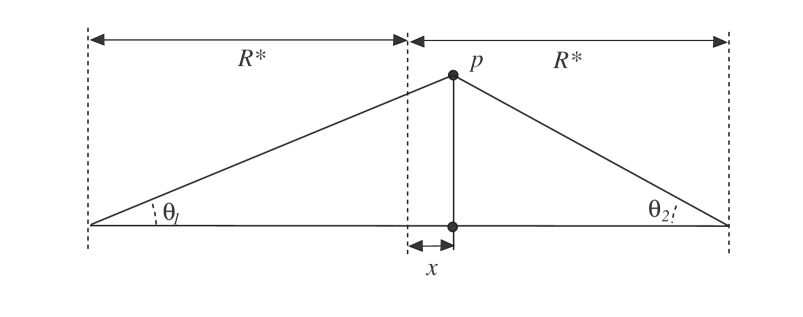
Figure 5.1: The solid angle $\theta_{1}+\theta_{2}$ of the hypercircular-based cone as a function of displacement $x$ from center of $p$.

To get this lower bound, we need to derive a worst-case scenario for $p$ and $K$ that makes $K_{p}$ as small as possible. Suppose $p$ has minimal distance $\delta$ from the boundary of $K$. Thus, the ball $B(p,\delta)$ intersects $K$ only at one point $k^{*}\in K$. Consider the hyperplane $H:=\{x:(p-k^{*})^{T}x=(p-k^{*})^{T}k^{*}\}$; it is tangent to $B(p,\delta)$ at $k^{*}$. No point $k$ in $K$ is on the same side of $H$ as $p$ (that is, satisfies $(p-k^{*})^{T}k>(p-k^{*})^{T}k^{*}$), else the line from $k$ to $k^{*}$ would contain points in $K$ that intersect $B(p,\delta)$ and hence contradict the minimality of the distance from $p$ to $k^{*}$. If we let

$$K^{*}:=B(\bar{0},R)\cap\{x:(p-k^{*})^{T}x\leq(p-k^{*})^{T}k^{*}\},$$

then we have shown that $K\subset K^{*}$. Let $M_{p}^{*}$ be $\{c\in S_{n}:\hskip 5.69054ptc^{T}k<c^{T}p\hskip 5.69054pt\forall k\in K^{*}\}$. It follows that $M_{p}^{*}\subset M_{p}$. Finally, we show that if $p$ is centered next to the set $C^{*}:=H\cap B(\bar{0},R)$, the set $M_{p}^{*}$ is as small as possible. Note that $C^{*}$ is a hyperdisc of radius $R^{*}$, where $R^{*}\leq R$. Fig. 5.1 defines the angles $\theta_{1}$ and $\theta_{2}$ as a function of the displacement $x$ of $p$ from the center of $C^{*}$, for $x\in[0,R^{*}]$. For a lower bound on $M_{p}^{*}$, we want to minimise the sum $\theta_{1}+\theta_{2}$. Since $\partial\theta_{1}/\partial x<\partial\theta_{2}/\partial x$, this sum is minimised at $x=0$, that is, when $p$ is centered next to $C^{*}$. As well, the value of $R^{*}$ that minimises the sum is $R^{*}=R$. Define $M_{p}^{*\prime}$ with respect to $K^{*}$ just as $M_{p}^{\prime}$ was defined with respect to $K$. Since

$$M_{p}^{*\prime}\subset M_{p}^{*}\subset M_{p},$$

calculating a lower bound on the size of $M_{p}^{*\prime}$ is sufficient. Below, instead of working with $K^{*}$ explicitly, we assume the worst case where $K$ is $K^{*}$ with $R^{*}=R$ and $p$ centered next to $C^{*}$.

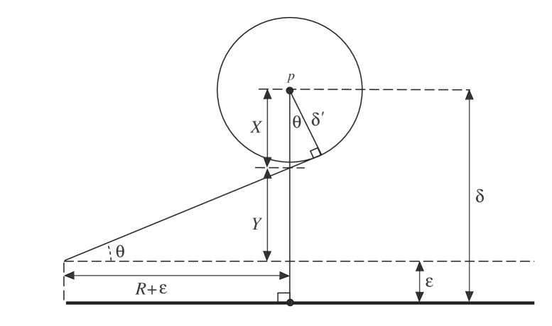
Figure 5.2: Derivation of solid angle $2\theta$ of hypercircular-based cone in terms of $R$ and $\delta$.

The angle $\theta$ can be seen in Fig. 5.2. We have

$$\tan\theta = \frac{Y}{R+\epsilon}$$

$$\cos\theta = \frac{\delta^{\prime}}{X}$$

$$2\delta^{\prime}=X+Y = (R+\epsilon)\tan\theta+\frac{\delta^{\prime}}{\cos\theta}$$

so that

$$\tan\theta=\frac{\delta^{\prime}}{R+\epsilon}(2-1/\cos\theta)$$ (5.31)

or

$$\sin\theta=\frac{\delta^{\prime}}{R+\epsilon}\left(2\cos\theta-1\right).$$ (5.32)

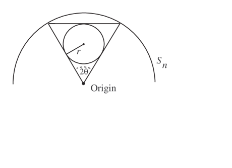
Figure 5.3: Derivation of radius $r$ as a function of $\theta$.

Now, we derive $r$ as a lower bound on the maximum radius of a ball that fits inside the hypercircular-based cone defined by $\theta$. From Fig. 5.3, we have

$$r=\sin\theta\tan\left(\frac{\pi}{4}-\frac{\theta}{2}\right).$$

Since $\tan(\upsilon-\psi)=(\tan\upsilon-\tan\psi)/(1+\tan\upsilon\tan\psi)$,

$$r=\sin\theta\frac{1-\tan(\theta/2)}{1+\tan(\theta/2)}.$$ (5.33)

As $\delta\rightarrow 0$ (and hence $\delta^{\prime},\epsilon\rightarrow 0$), equation (5.31) tends to $\tan\theta=\delta^{\prime}/R$ and equation (5.33) tends to $r=2\delta/5R$. For convenience of exposition, we use the approximation $r\approx 2\delta/5R$. In practice, equation (5.33) (in conjunction with a numerical solution for $\theta$) may be used in the derivation of Stopping Conditions 1 and 2.

5.3.4 Newton Iterates

The next theorem says that, with respect to $F$, the new (actual) analytic center and the old (approximate) analytic center are never too far apart, so that the Newton procedure for finding the new approximate analytic center terminates quickly (see the Appendix for a proof).

Theorem 35 (Theorem 20 in [91]).

There exists some constant $C_{\mathrm{d}}$ such that any time a hyperplane is discarded in Subcase 1.1, $F_{\mathrm{d}}(z)-F_{\mathrm{d}}(\omega_{\mathrm{d}})\leq C_{\mathrm{d}}$. Likewise, there exists some constant $C_{\mathrm{a}}$ such that any time a hyperplane is added in Case 2, $F_{\mathrm{a}}(z)-F_{\mathrm{a}}(\omega_{\mathrm{a}})\leq C_{\mathrm{a}}$.

In Subcase 1.1 or Case 2, to calculate new approximations $z_{\mathrm{new}}$ to the new analytic center $\omega_{\mathrm{new}}$, we perform damped Newton iterations, as defined in [95], starting at the old approximate analytic center $z$. Denote the sequence of ensuing Newton iterates by $\{x_{i}:i=0,1,\ldots\}$. The starting point is $x_{0}:=z$. Define $\lambda_{*}:=2-\sqrt{3}=0.2679...$. For $i\geq 0$, define the Newton iterates as:

$$x_{i+1}:=x_{i}-\varsigma_{i}(\nabla^{2}F(x_{i}))^{-1}\nabla F(x_{i}),$$

where

$$\varsigma_{i}:=\left\{\begin{array}[]{ll}(1+\lambda(x_{i}))^{-1}&\mbox{ if $\lambda(x_{i})\geq\lambda_{*}$ },\\ 1&\mbox{ if $\lambda(x_{i})<\lambda_{*}$}.\end{array}\right.$$

Theorem 2.2.3 in [95] shows that, in the first stage of the Newton process ($\lambda(x_{i})\geq\lambda_{*}$), the difference $F(x_{i})-F(x_{i+1})$ is at least $\lambda_{*}$ and, in the second stage of the Newton process ($\lambda(x_{i})<\lambda_{*}$), $\lambda(x_{i+1})<\lambda(x_{i})/2$. Thus, Theorem 35 says that, within $O(1)$ iterations, the value of $\lambda(x_{i})$ will start decreasing quadratically. The total number of Newton iterations required is no more than

$$\lceil{C_{\mathrm{d}}/\lambda_{*}}\rceil+\lceil{\log_{2}(\lambda_{*}/\rho_{0})}\rceil,$$

in Subcase 1.1, and

$$\lceil C_{\mathrm{a}}/\lambda_{*}\rceil+\lceil{\log_{2}(\lambda_{*}/\rho_{0})}\rceil,$$

in Case 2.

5.3.5 Selecting the Constants

Finally, we summarise the values of all the parameters of the algorithm and give values of the constants that work in general and for some special cases.

The parameters have been defined as follows:

$$r := 2\delta/5R$$

$$u := 2\log_{2}(n)+\log_{2}(1/r)$$

$$\tilde{\delta} := \delta^{\prime}/2R=\delta/5R.$$

For the constants, we have to summarise the strongest conditions that the convergence analysis placed on them:

$$\lambda(z) < 1/3$$

$$\tilde{\gamma} < 1/3$$

$$\zeta < 0.02\textrm{ [see proof of Theorem \ref{AV-thm11approx}, Case 2]}$$

$$C_{1} > 0$$

$$C_{2} > 0$$

$$C_{3} < 1/3\textrm{ [to invoke Lemma \ref{AV-lem6}]}$$

$$C_{4} < 0.615$$

$$C_{5} < 1\textrm{ [to invoke Lemma \ref{AV-lem5}]}$$

$$C_{6} > 0$$

$$3+(\log_{2}(12)+1/2)/2 < \frac{1}{2}\left(\nu\log_{2}(1+C_{2})-{\log_{2}(\nu)}\right).$$

The following list of values can be shown to satisfy the above constraints:

$$\rho_{0} := 0.001$$

$$\zeta_{0} := q_{\rho_{0}}=0.00101$$

$$\gamma_{0} := 0.25$$

$$\sigma_{0} := 0.08$$

$$\nu := 1078.$$

The potentially smallest upper bound imposed on $\zeta$ is

$$\zeta<\frac{\tilde{\delta}}{1+\tilde{\delta}}\frac{||z||}{\sqrt{2}},$$ (5.35)

in Lemma 33. We now show that this upper bound is never so small as to require an unreasonable number of Newton iterates, by deriving a lower bound on $||z||$ based on Stopping Condition 2. While Stopping Condition 2 is not satisfied, we have

$$2r<(a_{j}^{T}z-b_{j})(3\nu nu+4)/(1-\zeta_{0})\hskip 14.22636pt\forall j,$$

thus, in particular, for $j=1$,

$$||z||\geq a_{1}^{T}z>\frac{2r(1-\zeta_{0})}{3\nu nu+4}.$$

Thus the lowest upper bound ever imposed on $\zeta$ will be

$$\zeta<\frac{\tilde{\delta}}{1+\tilde{\delta}}\frac{\sqrt{2}r(1-\zeta_{0})}{3\nu nu+4}.$$ (5.36)

Let $t$ be the righthand side of the above inequality; note that $t$ is lower-bounded by a polynomial in $\frac{1}{n}$ and $\frac{\delta}{R}$. This gives a tight, worst-case upper bound on $\rho$ of $t-t^{2}+t^{3}/3$ which is still a polynomial in $\frac{1}{n}$ and $\frac{\delta}{R}$. Thus, in the worst case, the required number of Newton iterates is $O(\textrm{polylog}(n,\frac{R}{\delta}))$.

5.3.6 Tighter Stopping Conditions

The upper bound $(h+2)/2$ on $(1-||\omega||^{2})^{-1}$ in (5.15) is not tight because it throws away the entire summation in (5.3.1). Line (5.17) gives

$$||\omega||\leq||z||+\zeta_{0}\sqrt{\lambda_{\mathrm{max}}((\nabla^{2}F(z))^{-1})},$$

where $\lambda_{\mathrm{max}}((\nabla^{2}F(z))^{-1})$ is the largest eigenvalue of $(\nabla^{2}F(z))^{-1}$; which gives

$$(1-||\omega||^{2})^{-1}\leq\varpi(z):=\left(1-\left(||z||+\zeta_{0}\sqrt{\lambda_{\mathrm{max}}((\nabla^{2}F(z))^{-1})}\right)^{2}\right)^{-1}.$$

Recalling Lemma 24, Stopping Condition 2 can be immediately tightened to

$$2r>\frac{[\min_{i}\{a_{i}^{T}z-b_{i}\}]}{1-\zeta_{0}}(h+4\varpi(z)).$$

To tighten Stopping Condition 1, we go back to line (5.14), which gives

$$(x-\omega)^{T}\nabla^{2}F(\omega)(x-\omega)\leq h^{2}+h(8\varpi(z)-1)-16\varpi(z)+32\varpi(z)^{2}+2.$$

In conjunction with the proof of Lemma 28, we get

$$P\subset E(\nabla^{2}F(z),z,\vartheta^{\prime})$$

where

$$\vartheta^{\prime}:=\sqrt{2\left(\frac{h^{2}+h(8\varpi(z)-1)-16\varpi(z)+32\varpi(z)^{2}+2}{(1-\zeta_{0})^{2}}+\zeta_{0}^{2}\right)}.$$

Using this and Theorem 27, line (A.26) becomes

$$\frac{(2\vartheta^{\prime})^{n}}{2^{[\log_{2}((2.5)(1+C_{2})^{h-1})]/2-n/2}} < \left(\frac{r}{n}\right)^{n}$$

$$\frac{2\vartheta^{\prime}}{2^{[\log_{2}((2.5)(1+C_{2})^{h-1})]/2n-1/2}} < \frac{r}{n}$$

$$\log_{2}({2\vartheta^{\prime}})-\left[{\log_{2}((2.5)(1+C_{2})^{h-1})/2n-1/2}\right] < \log_{2}({r}/{n}),$$

to give the stopping condition

$$h>\frac{1}{\log_{2}(1+C_{2})}\left[2n\log_{2}({2n\vartheta^{\prime}}/{r})+n\right]+\log_{2}(4/5).$$

Employing these dynamic stopping conditions ensures that the number of calls to the WOPT oracle is minimised. When WOPT is NP-hard, as in the quantum separability problem, this is important in practice.

5.4 Complexity and Discussion

As in [91], we only ever have to compute $\sigma_{0}^{-1}n+1$ of the $\sigma_{i}(z)$ values, regardless of the number of hyperplanes $h$.

Theorem 36 (Theorem 21 in [91]).

In Case 1, if there is at least one hyperplane satisfying the conditions of Subcase 1.1, then we must discover such a hyperplane in at most $\sigma_{0}^{-1}n+1$ evaluations of the $\sigma_{j}(z)$ values.

Proof.

See [91]. ∎

The total arithmetic complexity of the algorithm is $O((T+n^{3}\log(R/\delta))n\log^{2}(nR/\delta))$, where $T$ is the cost of one call to WOPT. See [91] for a detailed discussion of the arithmetic complexity of the algorithm, including the complexity of calculating the inverse Hessians.

Note that – in the worst case – the algorithm requires more machine precision than the algorithm in [91] due to (5.36). However, I conjecture that, in the vast majority of instances, the magnitude $||z||$ of the approximate analytic center remains larger than a constant; hence the algorithm, which incorporates the dynamic bound (5.35), does not require excessive precision. Some evidence for this conjecture is based on the following result:

Fact 37.

If $b_{i}=0$ for all $i$, that is, if all cuts are central (through the origin, in our case), then, when a cut is added, the new analytic centre $\omega_{\mathrm{a}}$ is always bigger than the old analytic centre $\omega$; that is, $||\omega_{\mathrm{a}}||\geq||\omega||$.

Proof.

From left-multiplying $\nabla F(\omega)=0$ by $\omega^{T}$, we get

$$\frac{||\omega||^{2}}{1-||\omega||^{2}}=\frac{1}{2}\sum_{i=1}^{h}\frac{a_{i}^{T}\omega}{a_{i}^{T}\omega-b_{i}}=\frac{1}{2}\sum_{i=1}^{h}\frac{a_{i}^{T}\omega}{a_{i}^{T}\omega}=h/2.$$ (5.37)

Similarly, we get

$$\frac{||\omega_{\mathrm{a}}||^{2}}{1-||\omega_{a}||^{2}}=(h+1)/2.$$ (5.38)

Since the quantity ${||\omega||^{2}}/{(1-||\omega||^{2})}$ increases as $||\omega||$ increases (and similarly for $||\omega_{\mathrm{a}}||$), we have $||\omega_{\mathrm{a}}||\geq||\omega||$. ∎

Thus, if all the cutting planes go through the origin (all $b_{j}=0$), then the analytic center of $P$ grows in magnitude with each additional cutting plane. Since the shifts $b_{j}$ of the cutting planes tend to zero as the algorithm proceeds (because the eigenvalues of $(\nabla^{2}F(z))^{-1}$ tend to zero), the behaviour of the analytic center tends to the case of all cutting planes going through the origin. If the requirement for shallow cutting in [91] could be removed somehow, then our algorithm would be free of this worst case. It is an open problem whether there exists a polynomial-time, analytic centre algorithm for the convex feasibility problem that does not require shallow cutting.

With respect to the number of calls to WOPT, how might the algorithm compare with the unmodified analytic centre algorithm of [91] applied to $Q_{p}$ and (a weakened) $\text{SEP}_{Q_{p}}$ (as outlined in Section 4.5)? The new cut-generation rule elegantly combines the routine $\text{SEP}_{K^{\star}}$ and the constraint $\{c:p^{T}c\geq 1\}$.

Problem 9.

Analyse, and compare more carefully, the two cut-generation rules.

I have shown that the Atkinson-Vaidya algorithm works with an initial bounding sphere, in place of a hyperbox. This result means that we can use this modified algorithm with $\text{SEP}_{K^{\star}}$ and initial outer approximation equal to

$$P_{0}=B(\bar{0},R^{\star})\cap\{c:p^{T}c\geq 1\},$$ (5.39)

where $R^{\star}$ is the radius of the smallest origin-centred ball that contains the polar $K^{\star}$. Note that such a radius is available when the original set $K$ is known to contain a ball of radius $r_{0}$; in which case, $R^{\star}=1/r_{0}$. In the quantum separability problem, we have such a radius, given by the maximum separable ball centred at the maximally mixed state (see Section 1.2). Fact 15 gives the analytic centre of $P_{0}$ (note that if a hyperbox was used instead, the analytic centre may not be easily computable because of a lack of symmetry e.g. the centre is not necessarily a scalar multiple of $p$). This likely makes the standard method more efficient. Using this method with deep cuts may, in practice, yield the fastest fully polynomial algorithm.

5.5 Application to Quantum Separability Problem

We can handle two scenarios – one experimental, as described in Section 4.3, and the other theoretical. In the theoretical scenario, we assume that we know the density matrix for the given state $\rho\in\mathcal{D}_{M,N}$, but we do not know whether $\rho$ is separable; knowing the density matrix corresponds to having gathered all $M^{2}N^{2}-1$ independent expected values of the physical state $\rho$ in the experimental scenario. Since the algorithm finds an entanglement witness when $\rho$ is entangled, it could also be applied when $\rho$ is known to be entangled but an entanglement witness for $\rho$ is desired (though one may want to apply the entanglement witness optimization procedure [47] to the result of the algorithm, as our algorithm does not output optimal entanglement witnesses).

We characterise all potential entanglement witnesses for $\rho$ by

$$\mathcal{W}\equiv\{A\in\mathbb{H}_{M,N}:\textrm{tr}(A)=0,\textrm{tr}(A^{2})\leq 1\}.$$ (5.40)

For entangled $\rho$, define $\mathcal{W}_{\rho}$ to be the subset of $\mathcal{W}$ consisting of (right) entanglement witnesses that detect $\rho$; if $\rho$ is separable, then define $\mathcal{W}_{\rho}$ to be empty.

Let $\mathcal{B}=\{X_{i}:i=0,1,\ldots,M^{2}N^{2}-1\}$ be a basis as described in the beginning of Section 2.3. Let $j$ be the number of nontrivial expected values of $\rho$ that are known, $2\leq j\leq M^{2}N^{2}-1$; that is, (without loss) assume we know the expected values of the elements of $\mathcal{B}^{\prime}=\{X_{1},X_{2},\ldots,X_{j}\}$. The algorithm either finds an entanglement witness in $\textrm{span}(\mathcal{B}^{\prime})$ for $\rho$, or it concludes that no such witness exists.

For any $Y\in\mathbb{H}_{M,N}$ with $Y=\sum_{i=0}^{n-1}y_{i}X_{i}$, let $\overline{Y}$ be the $j$-dimensional vector of the real numbers $y_{i}$ for $i=1,2,\ldots,j$. Conversely, for any $\overline{Y}\in\mathbb{R}^{j}$ with elements $y_{1},\ldots,y_{j}$, let $Y=\sum_{i=1}^{j}y_{i}X_{i}$. Define the hyperplanes $\pi_{\overline{Y},b}=\{x\in\mathbb{R}^{j}:\overline{Y}^{T}x=b\}$ and halfspaces $H_{\overline{Y},b}=\{x\in\mathbb{R}^{j}:\overline{Y}^{T}x\leq b\}$ similarly to before. Define

$$\overline{S}_{M,N}=\{\overline{\sigma}:\sigma\in\mathcal{S}_{M,N}\}.$$ (5.41)

Note $\overline{S}_{M,N}$ is a convex set in $\mathbb{R}^{j}$ containing the origin. Define

$$\overline{\mathcal{W}} \equiv \{\overline{A}\in\mathbb{R}^{j}:A\in\mathcal{W}\}$$ (5.42)

$$\overline{\mathcal{W}}_{\rho} \equiv \{\overline{A}\in\overline{\mathcal{W}}:A\in\mathcal{W}_{\rho}\}.$$ (5.43)

Figure 5.4 shows a schematic of the sets $\mathcal{S}_{M,N}$, $\overline{S}_{M,N}$, $\overline{\mathcal{W}}$, and $\overline{\mathcal{W}}_{\rho}$.

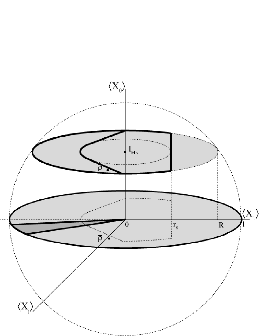
Figure 5.4: Schematic diagram (not to scale) of density operators and $\overline{\mathcal{W}}$ in $\mathbb{R}^{n}$, $n=M^{2}N^{2}$. The $\langle X_{1}\rangle-\langle X_{j}\rangle$ plane is a two-dimensional representation of the space $\textrm{span}(\{X_{1},X_{2},...,X_{j}\})$. The large dashed circle represents the origin-centered unit hypersphere in $\mathbb{R}^{n}$. The upper shaded ellipse represents the $(n-1)$-dimensional hyperball of radius $R$ centered at the maximally mixed state $I_{MN}$ which is the intersection of the hyperplane $\pi_{I,1}$ and the origin-centered unit hyperball in $\mathbb{R}^{n}$. The density operators are the heavy-outlined region in this $(n-1)$-dimensional hyperball; the inner heavy outlined shape represents the separable states $S_{M,N}$. The boundary of the maximal separable hyperball of radius $r_{S}$ centered at $I_{MN}$ is shown as a dashed ellipse. An entangled state $\rho$ is shown, and its projection $\overline{\rho}$ is also shown. The shaded elliptical disk (in heavy outline) in the $\langle X_{1}\rangle-\langle X_{j}\rangle$ plane is $\overline{\mathcal{W}}$ (i.e. is a representation of the origin-centered $(n-1)$-dimensional unit hyperball); the darker shaded wedge is $\overline{\mathcal{W}_{\rho}}$. The boundary of $\overline{S}_{M,N}$ is shown as a dashed line.

The algorithm solves the following problem:
Entanglement Witness Problem. Given the expected values of elements of $\mathcal{B}^{\prime}$ for $\rho\in\mathcal{D}_{M,N}$ and a precision parameter $\delta>0$, either assert

“$\overline{\rho}\in\overline{S}_{M,N}$”:	there exists a separable state $\sigma$
	such that $||\bar{\rho}-\bar{\sigma}||<\delta$; or return
$A\in\mathcal{W}$:	an operator such that
	$b^{*}(A)<tr(A\rho)$.

Note when $j=M^{2}N^{2}-1$, this problem solves the separability problem.

To reconcile the elements of the algorithm with the physics, note the following main correspondences:

$$n \sim j$$

$$K \sim \overline{S}_{M,N}$$

$$K_{p} \sim \overline{\mathcal{W}}_{\rho}(=\mathcal{W}_{\rho}\text{ if $j=M^{2}N^{2}-1$}).$$

To use this algorithm for the separability problem, it remains to show that there exists an appropriate centre $c_{0}$ and outer radius $R$ of $S_{M,N}$. The maximally mixed quantum state $I_{MN}=I/MN$ is properly contained in $S_{M,N}$ [15, 16], thus $c_{0}$ is the 0-vector in $\mathbb{R}^{j}$ corresponding to $I_{M,N}$:

$$c_{0}=(\textrm{tr}(X_{i}I_{M}N))_{i=1,...,j}=\begin{bmatrix}0\\ 0\\ \vdots\\ 0\end{bmatrix}\in\mathbb{R}^{j}.$$ (5.44)

We can calculate an upper bound $R$ on the radius of the smallest $c_{0}$-centered hypersphere that contains $\overline{S}_{M,N}$ by referring to Fig. 5.4. Because the space is Euclidean, we have $R=\sqrt{1-1/MN}$.

For the quantum separability problem, we can derive a slightly better lower bound $r$ than we could for the generic case in Section 5.3.3. This is easily done by making use of the radius $r_{S}=1/\sqrt{MN(MN-1)}$ of the largest separable hyperball centered at $I_{M,N}$ contained in $S_{M,N}$, which is derived in [16]. Using $r_{S}$, we no longer need to resort to using $R^{*}=R$; rather, we can use $R^{*}=\sqrt{R^{2}-r^{2}_{S}}$, as is easily seen from Fig. 5.4. The result is

$$r=\sin\theta\frac{1-\tan(\theta/2)}{1+\tan(\theta/2)},$$ (5.45)

where

$$\sin\theta=\frac{2\delta/5}{\sqrt{R^{2}-r^{2}_{S}}+\delta/5}\left(2\cos\theta-1\right).$$ (5.46)

5.6 Closing remarks

This chapter has given a new oracle-polynomial-time algorithm for WSEP($K$) relative to an oracle for WOPT($K$), for any convex $K\subset\mathbb{R}^{n}$ that properly contains a known point $c_{0}$ and is contained in a ball of finite known radius $R$. The novelty of the algorithm lies in the way in which the oracle is used to generate cutting planes for the feasibility problem for part of the polar of $K$. This new cut-generation method is based on an intuitive search heuristic (see Section 4.4).

The new algorithm is based heavily on the cutting-plane algorithm of Atkinson and Vaidya [91], which uses shallow cutting. I mentioned that it is an open problem whether there exists a polynomial-time, analytic centre algorithm for the convex feasibility problem that does not require shallow cutting. Actually, it has been suggested by John E. Mitchell [97] that central cutting can be used in the Atkinson-Vaidya algorithm, if certain techniques from [98] are employed to compute the new analytic centre. However, from correspondence with Mitchell and Yinyu Ye, it is unclear whether modifying the Atkinson-Vaidya algorithm in this way retains the polynomial-time convergence: while it is clear that a new analytic centre can be efficiently computed when central cuts are used, it is not clear that all the other delicate machinery in the convergence argument emerges unscathed.

Problem 10.

Can the Atkinson-Vaidya algorithm be modified so as not to require shallow cutting, while still being polynomial-time?

Combined with the material in Chapter 4, I have shown that the new algorithm has a real potential with regard to practical application to solving the quantum separability problem, both in theoretical and experimental contexts – the general strategy of reducing the problem to the optimisation problem is the best known (see Section 4.8). In the case where $M=N=2$, Ben Travaglione and I developed a working implementation of the algorithm, using Hansen’s interval-analysis global optimisation routine [85, 93]. This implementation runs fast enough that it could be used in practice. However, for higher dimensions (which are of greater interest and where precision and round-off considerations become extremely important), we were not satisfied that the implementation is optimal. Currently, Donny Cheung and I are working on a more robust implementation, which will hopefully run reasonably quickly in the case $M=N=3$; that is, the run time of the program on a separable state is hopefully on the order of hours or days, as opposed to years.

Appendix A Convergence proofs

Lemma 25 (Lemma 17 in [91]). Let $z$ be an approximation to $\omega$ such that $\omega\in E(\nabla^{2}F(z),z,\zeta)$. Suppose the hyperplane $(a,\beta)$ is added in Case 2 with $\gamma_{0}^{2}=\gamma^{2}=\frac{a^{T}(\nabla^{2}F(z))^{-1}a}{(a^{T}z-\beta)^{2}}$. Then,

$$\mathrm{(a)} \frac{|a^{T}(z-\omega)|}{a^{T}z-\beta}\leq\zeta\gamma,$$

$$\mathrm{(b)} \frac{|a^{T}(z-\omega)|}{a^{T}\omega-\beta}\leq\zeta\gamma/(1-\zeta\gamma),$$

$$\mathrm{(c)} \Psi_{\mathrm{a}}(\omega)\leq\tilde{\gamma}^{2}:=\gamma^{2}\left(\frac{1}{1-\zeta\gamma}\right)^{2}\left(\frac{1}{1-\zeta}\right)^{2}.$$

Proof.

(a) Since $\omega\in E(\nabla^{2}F(z),z,\zeta)$, we know that

$$|a^{T}(z-\omega)|\leq\zeta\sqrt{a^{T}(\nabla^{2}F(z))^{-1}a}.$$ (A.1)

Therefore,

$$\frac{|a^{T}(z-\omega)|}{a^{T}z-\beta}\leq\frac{\zeta\sqrt{a^{T}(\nabla^{2}F(z))^{-1}a}}{a^{T}z-\beta}=\zeta\gamma.$$ (A.2)

(b) By (A.1), we get

$$\frac{|a^{T}(z-\omega)|}{a^{T}\omega-\beta} \leq \frac{\zeta\sqrt{a^{T}(\nabla^{2}F(z))^{-1}a}}{a^{T}z-\beta+a^{T}(\omega-z)}$$ (A.3)

$$\leq \frac{\zeta\sqrt{a^{T}(\nabla^{2}F(z))^{-1}a}}{a^{T}z-\beta-\zeta\sqrt{a^{T}(\nabla^{2}F(z))^{-1}a}}=\frac{\zeta\gamma}{1-\zeta\gamma}.$$

(c)We have

$$\gamma^{2} = \frac{a^{T}(\nabla^{2}F(z))^{-1}a}{(a^{T}z-\beta)^{2}}$$

$$\geq (1-\zeta)^{2}\frac{a^{T}(\nabla^{2}F(\omega))^{-1}a}{(a^{T}z-\beta)^{2}}\hskip 5.69054pt[\textrm{by Lemma \ref{AV-cor4}}]$$

$$= (1-\zeta)^{2}\frac{a^{T}(\nabla^{2}F(\omega))^{-1}a/(a^{T}\omega-\beta)^{2}}{\left(1+a^{T}(z-\omega)/(a^{T}\omega-\beta)\right)^{2}}$$

$$\geq (1-\zeta)^{2}\frac{a^{T}(\nabla^{2}F(\omega))^{-1}a/(a^{T}\omega-\beta)^{2}}{(1+\zeta\gamma/(1-\zeta\gamma))^{2}}\hskip 5.69054pt[\textrm{from part (b)}]$$

$$= \frac{(1-\zeta)^{2}}{\left(1+\zeta\gamma/(1-\zeta\gamma)\right)^{2}}\nabla F_{\mathrm{a}}(\omega)^{T}(\nabla^{2}F(\omega))^{-1}\nabla F_{\mathrm{a}}(\omega)$$

$$\geq \frac{(1-\zeta)^{2}}{\left(1+\zeta\gamma/(1-\zeta\gamma)\right)^{2}}\underbrace{\nabla F_{\mathrm{a}}(\omega)^{T}(\nabla^{2}F_{\mathrm{a}}(\omega))^{-1}\nabla F_{\mathrm{a}}(\omega)}_{\Psi_{\mathrm{a}}(\omega)},$$

where the second-last line follows from $\nabla F_{\mathrm{a}}(\omega)=\nabla F(\omega)-a/(a^{T}\omega-\beta)=-a/(a^{T}\omega-\beta)$, and the last line follows by noting that $\nabla^{2}F_{\mathrm{a}}(x)=\nabla^{2}F(x)+aa^{T}/(a^{T}x-\beta)^{2}$ and applying Lemma 19. Thus,

$$\gamma^{2} \geq \frac{(1-\zeta)^{2}}{(1+\zeta\gamma/(1-\zeta\gamma))^{2}}\Psi_{\mathrm{a}}(\omega)$$ (A.4)

$$\Psi_{\mathrm{a}}(\omega) \leq \gamma^{2}\frac{1}{(1-\zeta\gamma)^{2}(1-\zeta)^{2}}=\tilde{\gamma}^{2}.$$

∎∎

Lemma 26 (Lemma 18 in [91]). Suppose a hyperplane is added in Case 2, and the analytic center moves from $\omega$ to $\omega_{\mathrm{a}}$. Let $\gamma=\sqrt{a^{T}(\nabla^{2}F(z))^{-1}a}/(a^{T}z-\beta)^{2}$. If $\tilde{\gamma}<\frac{1}{3}$, then

$$\frac{a^{T}(\nabla^{2}F(z))^{-1}a}{(a^{T}z_{\mathrm{a}}-\beta)^{2}}\geq\gamma^{2}\left(\frac{1-\zeta}{1+\gamma q_{\tilde{\gamma}}/(1-\zeta)+\zeta\gamma}\right)^{2}.$$

Proof.

We have

$$a^{T}z_{\mathrm{a}}-\beta = a^{T}z-\beta+a^{T}(z_{\mathrm{a}}-\omega_{\mathrm{a}}+\omega_{\mathrm{a}}-\omega+\omega-z)$$

$$\leq a^{T}z-\beta+|a^{T}(z_{\mathrm{a}}-\omega_{\mathrm{a}})|+|a^{T}(\omega_{\mathrm{a}}-\omega)|+|a^{T}(\omega-z)|$$

$$\leq a^{T}z-\beta+\underbrace{\zeta\sqrt{a^{T}(\nabla^{2}F_{\mathrm{a}}(z_{\mathrm{a}}))^{-1}a}}_{\textrm{by (\ref{AV-eqn65}) and Lemma \ref{AV-KKT}}}+\underbrace{q_{\tilde{\gamma}}\sqrt{a^{T}(\nabla^{2}F_{\mathrm{a}}(\omega))^{-1}a}}_{\textrm{by (\ref{AV-eqn81})}}$$

$$+\underbrace{\zeta\sqrt{a^{T}(\nabla^{2}F(z))^{-1}a}}_{\textrm{by (\ref{AV-eqn65}) and Lemma \ref{AV-KKT}}}$$

$$\leq a^{T}z-\beta+\zeta\sqrt{a^{T}(\nabla^{2}F_{\mathrm{a}}(z_{\mathrm{a}}))^{-1}a}+\underbrace{q_{\tilde{\gamma}}\sqrt{a^{T}(\nabla^{2}F(\omega))^{-1}a}}_{\textrm{by Lemma \ref{AV-cor4}}}$$

$$+\zeta\sqrt{a^{T}(\nabla^{2}F(z))^{-1}a}$$

$$\leq a^{T}z-\beta+\underbrace{\zeta(a^{T}z_{\mathrm{a}}-\beta)}_{\textrm{by Lemma \ref{AV-lem1}}}+q_{\tilde{\gamma}}\sqrt{a^{T}(\nabla^{2}F(\omega))^{-1}a}$$

$$+\zeta\sqrt{a^{T}(\nabla^{2}F(z))^{-1}a}.$$

And so,

$$\frac{a^{T}z_{\mathrm{a}}-\beta}{a^{T}z-\beta} \leq \frac{1}{1-\zeta}\left(1+q_{\tilde{\gamma}}\frac{\sqrt{a^{T}(\nabla^{2}F(\omega))^{-1}a}}{a^{T}z-\beta}+\frac{\zeta\sqrt{a^{T}(\nabla^{2}F(z))^{-1}a}}{a^{T}z-\beta}\right)$$ (A.5)

$$\leq \frac{1}{1-\zeta}\left(1+\underbrace{\frac{q_{\tilde{\gamma}}}{1-\zeta}\frac{\sqrt{a^{T}(\nabla^{2}F(z))^{-1}a}}{a^{T}z-\beta}}_{\textrm{by Lemmas \ref{AV-lem3} and \ref{AV-cor4}}}+\frac{\zeta\sqrt{a^{T}(\nabla^{2}F(z))^{-1}a}}{a^{T}z-\beta}\right)$$

$$= \frac{1}{1-\zeta}\left(1+\frac{q_{\tilde{\gamma}}}{1-\zeta}\gamma+\zeta\gamma\right)=\frac{1+\gamma q_{\tilde{\gamma}}/(1-\zeta)+\zeta\gamma}{1-\zeta}.$$

It now follows that

$$\frac{a^{T}(\nabla^{2}F(z))^{-1}a}{(a^{T}z_{\mathrm{a}}-\beta)^{2}} = \frac{a^{T}(\nabla^{2}F(z))^{-1}a}{(a^{T}z-\beta)^{2}}\frac{(a^{T}z-\beta)^{2}}{(a^{T}z_{\mathrm{a}}-\beta)^{2}}$$ (A.6)

$$\geq \gamma^{2}\left(\frac{1-\zeta}{1+\gamma q_{\tilde{\gamma}}/(1-\zeta)+\zeta\gamma}\right)^{2}$$

as stated in the lemma.∎∎

Theorem 27 (Approximation version of Theorem 13 in [91]). Suppose that $\max_{1\leq i\leq h}\mu_{i}(z)\leq 2$ at the beginning of an iteration, i.e. Case 2 is about to occur. If the current search space $P$ is determined by $h$ hyperplanes (in addition to the unit hypersphere), then

$$\mathrm{det}(\nabla^{2}F(z))>2^{-n}(1+C_{2})^{h}=2^{(\log_{2}(1+C_{2}))h-n},$$ (A.7)

for some positive constant $C_{2}$ which depends on the parameters $\sigma_{0}$ and $\gamma_{0}$ of the algorithm and the “minimal goodness” $\zeta_{0}$ of the approximation to the analytic centers. This can be improved to

$$\mathrm{det}(\nabla^{2}F(z))>2^{-n}(2.5)(1+C_{2})^{h-1}.$$ (A.8)

Proof.

Let $\{(a_{1},b_{1}),\ldots,(a_{h},b_{h})\}$ be the set of hyperplanes describing $P$. For each $i$, let $s_{i}$ be the number of the most recent iteration in which $\kappa(a_{i},b_{i}$) was changed. Without loss of generality, we assume that $s_{1}<s_{2}<\ldots<s_{h}$. Let $F_{0}(x)$ be our self-concordant barrier function over the hyperball alone:

$$\nabla^{2}F_{0}(x)=\frac{4xx^{T}}{(1-x^{T}x)^{2}}+\frac{2I}{(1-x^{T}x)}.$$ (A.9)

Construct a set of auxiliary matrices as follows:

$$M_{0}:=2I,\hskip 14.22636ptM_{i}:=M_{i-1}+\frac{a_{i}a_{i}^{T}}{(\kappa(a_{i},b_{i}))^{2}},\hskip 5.69054pti=1,\ldots h.$$ (A.10)

The matrix $M_{0}$ is $\nabla^{2}F_{0}(\bar{0})$. The $M_{i}$’s add in the terms corresponding to $(a_{i},b_{i})$ with the current settings of $\kappa(a_{i},b_{i})$.

Let $z(s_{k})$ represent the approximate analytic center at the beginning of iteration $s_{k}$. At the beginning of iteration $s_{k}$, the $\kappa$ values corresponding to constraints in the set $\{(a_{1},b_{1}),\ldots,(a_{k-1},b_{k-1})\}$ have already experienced their final change up to the time of the statement of the theorem. Because $\kappa(a_{k},b_{k})$ changes in the iteration $s_{k}$, iteration $s_{k}$ must be an occurrence of either Subcase 1.2 or Case 2. If it is an occurrence of Case 2, then we easily see that

$$a_{i}^{T}z(s_{k})-b_{i}\leq 2\kappa(a_{i},b_{i}),\hskip 5.69054pti=1,\ldots,k-1,$$ (A.11)

for otherwise Case 2 would not occur at all. Inequality (A.11) also holds true, however, if iteration $s_{k}$ is an occurrence of Subcase 1.2, for the following reason: Suppose that, for some $\hat{\iota}$ in $\{1,\ldots k-1\}$, $a^{T}_{\hat{\iota}}z(s_{k})-b_{\hat{\iota}}>2\kappa(a_{\hat{\iota}},b_{\hat{\iota}})$. Notice that Subcase 1.2 does not affect the approximate analytic center at all, and no plane is in line to be discarded, else Subcase 1.1 would occur instead of Subcase 1.2. As a result, instances of Subcase 1.2 continue to occur until $\kappa(a_{\hat{\iota}},b_{\hat{\iota}})$ becomes reset. This contradicts the assumption that, at iteration $s_{k}$, the $\hat{\iota}$th $\kappa$-value has experienced its last change. So, regardless of whether iteration $s_{k}$ is an instance of Subcase 1.2 or Case 2, inequality (A.11) holds, and, therefore,

$$\frac{1}{(a^{T}_{i}z(s_{k})-b_{i})^{2}}\geq\frac{1}{4(\kappa(a_{i},b_{i}))^{2}},\hskip 5.69054pti=1,\ldots,k-1.$$ (A.12)

Since the Hessian of the barrier function $F$ takes the form

$$\nabla^{2}F(z(s_{k})) = \frac{4z(s_{k})z(s_{k})^{T}}{(1-z^{T}(s_{k})z(s_{k}))^{2}}+\frac{2I}{1-z^{T}(s_{k})z(s_{k})}+\sum_{i=1}^{k-1}\frac{a_{i}a_{i}^{T}}{(a_{i}^{T}z(s_{k})-b_{i})^{2}}$$ (A.13)

$$+(\textrm{additional positive semi-definite terms}),$$

it follows that at the beginning of iteration $s_{k}$ we have

$$\xi^{T}\nabla^{2}F(z(s_{k}))\xi \geq \xi^{T}M_{0}\xi+\sum_{i=1}^{k-1}\frac{(a_{i}^{T}\xi)^{2}}{4(\kappa(a_{i},b_{i}))^{2}}$$ (A.14)

$$\geq \frac{\xi^{T}M_{0}\xi}{4}+\sum_{i=1}^{k-1}\frac{(a_{i}^{T}\xi)^{2}}{4(\kappa(a_{i},b_{i}))^{2}}$$

$$= \frac{1}{4}\xi^{T}M_{k-1}\xi,\hskip 5.69054pt\textrm{for every $\xi\in\mathbf{R}^{n}$.}$$

(The two terms corresponding to the hypersphere are minimised when $z=\bar{0}$, which is the setting of $z$ in our definition of $M_{0}$.) Thus, by Lemma 19,

$$\xi^{T}(\nabla^{2}F(z(s_{k})))^{-1}\xi\leq 4\xi^{T}M_{k-1}^{-1}\xi,\hskip 5.69054pt\textrm{for every $\xi\in\mathbf{R}^{n}$}.$$

Iteration $s_{k}$ is the last time $\kappa(a_{k},b_{k})$ was changed, and this change occurred in Subcase 1.2 or Case 2. If the change occurred in Subcase 1.2, then, at the time of the change,

$$\sigma_{0} \leq \frac{a^{T}_{k}(\nabla^{2}F(z(s_{k})))^{-1}a_{k}}{(a_{k}^{T}z(s_{k})-b_{k})^{2}}\hskip 14.22636pt\textrm{[by definition of $\sigma_{k}$]}$$

$$\leq 4\frac{a^{T}_{k}(M_{k-1})^{-1}a_{k}}{(a_{k}^{T}z(s_{k})-b_{k})^{2}}=4\frac{a^{T}_{k}(M_{k-1})^{-1}a_{k}}{(\kappa(a_{k},b_{k}))^{2}}$$

($\kappa(a_{k},b_{k})$ is the newly reset value) and we conclude that

$$\frac{a_{k}^{T}(M_{k-1})^{-1}a_{k}}{(\kappa(a_{k},b_{k}))^{2}}\geq\frac{\sigma_{0}}{4}.$$ (A.15)

If the change occurred in Case 2, then the argument is harder. We employ the notation $(a,\beta)$ to refer to the hyperplane added in Case 2, just as we did in the algorithm itself. By Lemma 26, if $\tilde{\gamma}<\frac{1}{3}$, then

$$\frac{a^{T}(\nabla^{2}F(z(s_{k})))^{-1}a}{(a^{T}z_{\mathrm{a}}-\beta)^{2}}\geq\gamma^{2}\left(\frac{1-\zeta}{1+\gamma q_{\tilde{\gamma}}/(1-\zeta)+\zeta\gamma}\right)^{2}.$$ (A.16)

Thus, since we set $\beta$ to make $\gamma^{2}=\gamma_{0}^{2}$,

$$\frac{a^{T}(\nabla^{2}F(z(s_{k})))^{-1}a}{(a^{T}z_{\mathrm{a}}-\beta)^{2}}\geq C_{1}:=\gamma_{0}^{2}\left(\frac{1-\zeta_{0}}{1+\gamma_{0}q_{\tilde{\gamma_{0}}}/(1-\zeta_{0})+\zeta\gamma_{0}}\right)^{2},$$ (A.17)

where $\tilde{\gamma_{0}}:=\gamma_{0}^{2}\left({1}/(1-\zeta_{0}\gamma_{0})\right)^{2}\left({1}/(1-\zeta_{0})\right)^{2}$, consequently,

$$C_{1}\leq\frac{a^{T}(\nabla^{2}F(z(s_{k})))^{-1}a}{(a^{T}z_{\mathrm{a}}-\beta)^{2}}\leq 4\frac{a^{T}(M_{k-1})^{-1}a}{(a^{T}z_{\mathrm{a}}-\beta)^{2}}=4\frac{a^{T}(M_{k-1})^{-1}a}{(\kappa(a,\beta))^{2}},$$ (A.18)

and it follows that

$$\frac{a^{T}(M_{k-1})^{-1}a}{(\kappa(a,\beta))^{2}}\geq\frac{C_{1}}{4}.$$ (A.19)

Regardless of whether the change of $\kappa(a_{k},b_{k})$ occurs in Subcase 1.2 or in Case 2, from (A.15) and (A.19) we can assert that

$$\frac{a_{k}^{T}(M_{k-1})^{-1}a_{k}}{(\kappa(a_{k},b_{k}))^{2}}\geq C_{2}:=\frac{1}{4}\min\{\sigma_{0},C_{1}\},\hskip 14.22636pt\textrm{for $1\leq k\leq h$.}$$ (A.20)

In fact, since we add the first cutting plane $(a_{1},0)$ “manually”, we know that, for $k=1$,

$$\frac{a_{1}^{T}(M_{0})^{-1}a_{1}}{(\kappa(a_{1},b_{1}))^{2}}=\frac{1/2}{1/{3}}=3/2=1.5,$$ (A.21)

where $1.5$ may be larger than the largest $C_{2}$ we can achieve.

Since each $M_{i}$, $i=1,\ldots,h$ is symmetric positive definite, we have, for $i\geq 1$,

$$\det(M_{i}) = \det(M_{i-1}+a_{i}a_{i}^{T}/(\kappa(a_{i},b_{i}))^{2})$$

$$= \det\left((M_{i-1})^{1/2}\left(I+\frac{(M_{i-1})^{-1/2}a_{i}a_{i}^{T}(M_{i-1})^{-1/2}}{(\kappa(a_{i},b_{i}))^{2}}\right)(M_{i-1})^{1/2}\right)$$

$$= \det(M_{i-1})\det\left(I+\frac{(M_{i-1})^{-1/2}a_{i}a_{i}^{T}(M_{i-1})^{-1/2}}{(\kappa(a_{i},b_{i}))^{2}}\right)$$

For an arbitrary vector $v\in\mathbf{R}^{n}$, the operator $(I\pm vv^{T})$ has set of eigenvalues $\{1,1,\ldots,1\pm v^{T}v\}$. Thus, for $i\geq 1$,

$$\det(M_{i}) = \det(M_{i-1})\left(1+\frac{a^{T}_{i}(M_{i-1})^{-1}a}{(\kappa(a_{i},b_{i}))^{2}}\right)$$

$$\geq \det(M_{i-1})(1+C_{2}).$$

Therefore, we have

$$\det(M_{h}) \geq (\det M_{0})(1+C_{2})^{h}$$ (A.22)

$$= 2^{n}(1+C_{2})^{h}.$$ (A.23)

The hypotheses of the theorem state that Case 2 is about to occur. This means that (A.11) and (A.12) hold at the current $z$ and for $h\geq 1$. Likewise, (A.14) is true with the current $z$ in place of $z(s_{k})$ and with $h$ in place of $k-1$, i.e., we have $\xi^{T}\nabla^{2}F(z)\xi\geq\frac{1}{4}\xi^{T}M_{h}\xi$ for all $\xi$. Thus,

$$\det(\nabla^{2}F(z))\geq\frac{1}{4^{n}}\det(M_{h}),$$

and so

$$\det(\nabla^{2}F(z))\geq\frac{1}{4^{n}}\cdot 2^{n}\cdot(1+C_{2})^{h}=2^{-n}(1+C_{2})^{h},$$

which proves the theorem. Alternatively, taking potential advantage of (A.21),

$$\det(\nabla^{2}F(z))\geq 2^{-n}(2.5)(1+C_{2})^{h-1}.$$ (A.24)

∎∎

Lemma 28 (Lemma 19 in [91]). For the approximate analytic center $z$ with $\omega\in E(\nabla^{2}F(z),z,\zeta)$, we have

$$P\subset E(\nabla^{2}F(z),z,\vartheta),$$

where

$$\vartheta := \sqrt{2\left(\frac{14h^{2}}{(1-\zeta)^{2}}+\zeta^{2}\right)},\hskip 14.22636pt\textrm{if $h>31$.}$$

Proof.

For every $x\in P$,

$$(x-z)^{T}\nabla^{2}F(z)(x-z)$$

$$= (x-\omega+\omega-z)^{T}\nabla^{2}F(z)(x-\omega+\omega-z)$$

$$= (x-\omega)^{T}\nabla^{2}F(z)(x-\omega)+(\omega-z)^{T}\nabla^{2}F(z)(\omega-z)+2(x-\omega)^{T}\nabla^{2}F(z)(\omega-z)$$

$$\leq 2(x-\omega)^{T}\nabla^{2}F(z)(x-\omega)+2(\omega-z)^{T}\nabla^{2}F(z)(\omega-z),\hskip 14.22636pt[\textrm{since $2a\cdot b\leq a\cdot a+b\cdot b$}]$$

$$\leq 2(x-\omega)^{T}\frac{\nabla^{2}F(\omega)}{(1-\zeta)^{2}}(x-\omega)+2\zeta^{2}\hskip 14.22636pt[\textrm{by Lemma \ref{AV-lem3} and hypothesis}].$$

The lemma follows by substituting the conclusion of Lemma 23 for $(x-\omega)^{T}{\nabla^{2}F(\omega)}(x-\omega)$.∎∎

Theorem 29 (Approximation version of Theorem 14 in [91]). There exists a constant $\nu$, independent of $h$, $n$, $R$, and $\delta$, and there exists a function $u(n,\delta)\in\Theta(\mathrm{poly}(n,\log(\frac{R}{\delta})))$ such that if $h=\nu nu(n,\delta)$, then the volume of $K_{p}$ is sufficiently small so as to assert that $p\in S(K,\delta)$.

Proof.

The volume of an ellipsoid $E(A,z,r)$ is upper-bounded by $r^{n}2^{n}/\sqrt{\det A}$ [1]. Thus, from Lemma 28,

$$\mathrm{volume}(P)\leq\mathrm{volume}(E(\nabla^{2}F(z),z,6h))\leq\frac{(12h)^{n}}{\sqrt{\det\nabla^{2}F(z)}}.$$

To prove the theorem, the bound in (5.7) implies that it suffices to show that there exists $\nu$ and $u$ such that $h=\nu nu$ implies

$$\frac{(12\nu nu)^{n}}{\sqrt{\det\nabla^{2}F(z)}}<\left(\frac{r}{n}\right)^{n}.$$ (A.25)

Theorem 27 strengthens this further to

$$\frac{(12\nu nu)^{n}}{2^{[\log_{2}(1+C_{2})]\nu nu/2-n/2}} < \left(\frac{r}{n}\right)^{n}$$ (A.26)

$$\frac{12\nu nu}{2^{[\log_{2}(1+C_{2})]\nu u/2-1/2}} < \frac{r}{n}$$ (A.27)

$$\log_{2}(12\nu nu)-({{[\log_{2}(1+C_{2})]\nu u/2-1/2}}) < \log_{2}(r/n)$$

$$\log_{2}(n/r)+\log_{2}(n)+\log_{2}(u)+\log_{2}(12)+1/2 < \nu u\log_{2}(1+C_{2})/2-\log_{2}(\nu)$$

$$\frac{\log_{2}(n/r)}{u}+\frac{\log_{2}(n)}{u}+\frac{\log_{2}(u)}{u}+\frac{\log_{2}(12)+1/2}{u} < \nu\log_{2}(1+C_{2})/2$$ (A.28)

$$-\frac{\log_{2}(\nu)}{u}.$$

Setting

$$u:=\log_{2}(n/r)+\log_{2}(n)=2\log_{2}(n)+\log_{2}(1/r)$$ (A.29)

and assuming $n\geq 2$ gives $u\geq 2$ and hence an upper bound on the left side of (A.28) of $1+1+1+(\log_{2}(12)+1/2)/2\leq 5.0424$. Thus it suffices to find $\nu$ such that

$$5.0424<\frac{1}{2}(\nu\log_{2}(1+C_{2})-{\log_{2}(\nu)}).$$ (A.30)

Since $C_{2}$ is a constant, it suffices that $\nu$ be constant. Later we will see that $r$ is roughly $\delta/R$, thus the theorem is proven. The higher the value of $C_{2}$, the smaller the value $\nu$ that we need. Note that the constant $\nu$ may be improved (lowered) with knowledge of $r$ and for specific (larger) values of $n$.∎∎

Lemma 30 (Lemma 16 in [91]). Let $\zeta<1$. If $\omega\in E(\nabla^{2}F(z),z,\zeta)$, then for all $i$, $1\leq i\leq h$,

$$\sigma_{i}(\omega)\leq\frac{\sigma_{i}(z)}{(1-\zeta)^{4}}.$$ (A.31)

Proof.

From Lemmas 18 and 19, we know that for all $\xi\in\mathbf{R}^{n}$

$$\frac{1}{(1-\zeta)^{2}}\xi^{T}(\nabla^{2}F(z))^{-1}\xi\geq\xi^{T}(\nabla^{2}F(\omega))^{-1}\xi\geq(1-\zeta)^{2}\xi^{T}(\nabla^{2}F(z))^{-1}\xi.$$

Therefore,

$$\sigma_{i}(\omega) = \frac{a^{T}_{i}(\nabla^{2}F(\omega))^{-1}a_{i}}{(a_{i}^{T}\omega-b_{i})^{2}}\leq\frac{1}{(1-\zeta)^{2}}\frac{a^{T}_{i}(\nabla^{2}F(z))^{-1}a_{i}}{(a_{i}^{T}\omega-b_{i})^{2}}$$ (A.32)

$$= \frac{1}{(1-\zeta)^{2}}\frac{a^{T}_{i}(\nabla^{2}F(z))^{-1}a_{i}/(a_{i}^{T}z-b_{i})^{2}}{[(a_{i}^{T}\omega-b_{i})/(a_{i}^{T}z-b_{i})]^{2}}$$

$$= \frac{1}{(1-\zeta)^{2}}\frac{a^{T}_{i}(\nabla^{2}F(z))^{-1}a_{i}/(a_{i}^{T}z-b_{i})^{2}}{[1+a_{i}^{T}(\omega-z)/(a_{i}^{T}z-b_{i})]^{2}}$$

$$= \frac{1}{(1-\zeta)^{2}}\frac{\sigma_{i}(z)}{[1+a_{i}^{T}(\omega-z)/(a_{i}^{T}z-b_{i})]^{2}}.$$

We know from Lemma 16 that $\zeta\sqrt{a^{T}_{i}(\nabla^{2}F(z))^{-1}a_{i}}\geq|a_{i}^{T}(\omega-z)|$, and therefore

$$\frac{|a_{i}^{T}(\omega-z)|}{|a_{i}^{T}z-b_{i}|}\leq\zeta\frac{\sqrt{a_{i}^{T}(\nabla^{2}F(z))^{-1}a_{i}}}{a_{i}^{T}z-b_{i}}\leq\zeta,$$ (A.33)

where the second inequality follows since $P\in E(\nabla^{2}F(z),z,1)$ (by Lemma 17) and hence $\sqrt{a_{i}^{T}(\nabla^{2}F(z))^{-1}a_{i}}\leq a_{i}^{T}z-b_{i}$. It follows that

$$\sigma_{i}(\omega)\leq\frac{1}{(1-\zeta)^{2}}\frac{\sigma_{i}(z)}{(1-\zeta)^{2}}=\frac{\sigma_{i}(z)}{(1-\zeta)^{4}}.$$

∎∎

Theorem 31 (Approximation version of Theorem 11 in [91]). There exists a positive constant $\theta$, independent of $h$, $n$, $R$, and $\delta$, such that after $\iota$ iterations of the algorithm, $N(\omega)\geq\theta\iota$. The constant $\theta$ will depend on the parameters of the algorithm.

Proof.

The proof is a case analysis following the different cases in the algorithm.

Case 1, Subcase 1.1: Let $F_{\mathrm{d}}(x)$, $\Psi_{\mathrm{d}}(x)$, and $N_{\mathrm{d}}(x)$ denote the functions $F(x)$, $\Psi(x)$, and $N(x)$ resulting after a hyperplane is dropped. We have immediately that

$$N_{\mathrm{d}}(z)\geq N(z)+\ln 2.$$ (A.34)

This is because by discarding a hyperplane, we have eliminated a term from (5.23) that is known to be less than or equal to $-\ln 2$. In this subcase, however, we must consider the effect of moving to a new approximate analytic center $z_{\mathrm{d}}$. It works against us that, after the drop, $N_{\mathrm{d}}(\omega)\geq N_{\mathrm{d}}(\omega_{\mathrm{d}})$. Our goal, however, is to show that the difference is small relative to the guaranteed $\ln 2$ increase.

We know

$$(\nabla F_{\mathrm{d}}(\omega))^{T}=\underbrace{(\nabla F(\omega))^{T}}_{=0}+\frac{a^{T}_{j}}{a^{T}_{j}\omega-b_{j}}=\frac{a^{T}_{j}}{a^{T}_{j}\omega-b_{j}}$$ (A.35)

and

$$\nabla^{2}F_{\mathrm{d}}(\omega)=\nabla^{2}F(\omega)-\frac{a_{j}a^{T}_{j}}{(a^{T}_{j}\omega-b_{j})^{2}}.$$ (A.36)

Since $\nabla^{2}F(\omega)$ is symmetric positive definite, it has a square root, and hence

$$\nabla^{2}F_{\mathrm{d}}(\omega) = (\nabla^{2}F(\omega))^{\frac{1}{2}}\left[I-\frac{(\nabla^{2}F(\omega))^{-\frac{1}{2}}a_{j}a_{j}^{T}(\nabla^{2}F(\omega))^{-\frac{1}{2}}}{(a^{T}_{j}\omega-b_{j})^{2}}\right]$$ (A.37)

$$\times(\nabla^{2}F(\omega))^{\frac{1}{2}}.$$

For an arbitrary vector $v\in\mathbf{R}^{n}$, the operator $(I-vv^{T})$ has set of eigenvalues $\{1,1,\ldots,1-v^{T}v\}$. If $v^{T}v<1$ then $(I-vv^{T})>0$, and for all $\xi\in\mathbf{R}^{n}$,

$$(1-v^{T}v)\xi^{T}\xi\leq\xi^{T}(1-vv^{T})\xi\leq\xi^{T}\xi.$$ (A.38)

We can apply equation (A.38) to the inner matrix in (A.37) with

$$v:=(\nabla^{2}F(\omega))^{-\frac{1}{2}}a_{j}/(a_{j}^{T}\omega-b_{j})$$

and with $\xi:=(\nabla^{2}F(\omega))^{\frac{1}{2}}\chi$ to conclude that for every $\chi\in\mathbf{R}^{n}$,

$$(1-\sigma_{j}(\omega))\chi^{T}\nabla^{2}F(\omega)\chi\leq\chi^{T}\nabla^{2}F_{\mathrm{d}}(\omega)\chi\leq\chi^{T}\nabla^{2}F(\omega)\chi$$ (A.39)

and thus by Corollary 19, for every $\chi\in\mathbf{R}^{n}$

$$\frac{1}{1-\sigma_{j}(\omega)}\chi^{T}(\nabla^{2}F(\omega))^{-1}\chi\geq\chi^{T}(\nabla^{2}F_{\mathrm{d}}(\omega))^{-1}\chi\geq\chi^{T}(\nabla^{2}F(\omega))^{-1}\chi.$$ (A.40)

The substitution $\chi:=\nabla^{2}F_{\mathrm{d}}(\omega)$ gives by equation (A.35)

$$\frac{\sigma_{j}(\omega)}{1-\sigma_{j}(\omega)} \geq \Psi_{\mathrm{d}}(\omega)\geq\sigma_{j}(\omega).$$

Since in this Subcase 1.1 we have $\sigma_{j}(z)<\sigma_{0}$, Lemma 30 gives

$$\sigma_{j}(\omega)\leq\frac{\sigma_{j}(z)}{(1-\zeta)^{4}}<\frac{\sigma_{0}}{(1-\zeta)^{4}}.$$ (A.41)

We then have

$$\Psi_{\mathrm{d}}(\omega)\leq\frac{\sigma_{j}(\omega)}{1-\sigma_{j}(\omega)}<\frac{\sigma_{0}/(1-\zeta)^{4}}{1-\sigma_{0}/(1-\zeta)^{4}},$$

or,

$$\lambda_{\mathrm{d}}(\omega):=\sqrt{\Psi_{\mathrm{d}}(\omega)}<C_{3}:=\sqrt{\frac{\sigma_{0}/(1-\zeta_{0})^{4}}{1-\sigma_{0}/(1-\zeta_{0})^{4}}}.$$ (A.42)

It thus follows from Lemma 21 that

$$F_{\mathrm{d}}(\omega)-F_{\mathrm{d}}(\omega_{\mathrm{d}})<C_{4}:=\frac{1}{2}q_{C_{3}}^{2}\left(\frac{1+q_{C_{3}}}{1-q_{C_{3}}}\right),$$ (A.43)

and consequently $N_{\mathrm{d}}(\omega)-N_{\mathrm{d}}(\omega_{\mathrm{d}})<C_{4}$. Now,

$$N_{\mathrm{d}}(\omega_{\mathrm{d}})-N(\omega) = (N_{\mathrm{d}}(\omega_{\mathrm{d}})-N_{\mathrm{d}}(\omega))+(N_{\mathrm{d}}(\omega)-N_{\mathrm{d}}(z))$$ (A.44)

$$+(N_{\mathrm{d}}(z)-N(z))+(N(z)-N(\omega))$$

$$= (N_{\mathrm{d}}(\omega_{\mathrm{d}})-N_{\mathrm{d}}(\omega))+\left(N(\omega)-N(z)+\ln\left(\frac{a_{i}^{T}\omega-b_{i}}{a_{i}^{T}z-b_{i}}\right)\right)$$

$$+(N_{\mathrm{d}}(z)-N(z))+(N(z)-N(\omega))$$

$$= (N_{\mathrm{d}}(\omega_{\mathrm{d}})-N_{\mathrm{d}}(\omega))+(N_{\mathrm{d}}(z)-N(z))+\ln\left(\frac{a_{i}^{T}\omega-b_{i}}{a_{i}^{T}z-b_{i}}\right)$$

$$\geq -C_{4}+\ln 2+\ln\left(1+\frac{a_{i}^{T}(\omega-z)}{a_{i}^{T}z-b_{i}}\right)$$

$$\geq -C_{4}+\ln 2+\ln\left(1-\frac{|a_{i}^{T}(\omega-z)|}{|a_{i}^{T}z-b_{i}|}\right)$$

$$> -C_{4}+\ln 2+\ln\left(1-\zeta\right)\hskip 14.22636pt\textrm{[see (\ref{AV-eqn69})]}$$

$$> -C_{4}+\ln 2-\zeta-4\zeta^{2}\hskip 14.22636pt\textrm{[assuming $\zeta<\frac{1}{2}$]}$$

$$> -C_{4}+0.615\hskip 14.22636pt\textrm{[assuming $\zeta<\frac{1}{16}$].}$$

Thus, as long as $C_{4}<0.615$, the theorem is proven in Subcase 1.1.

Case 1, Subcase 1.2: The only action in this subcase is a change in $\kappa(a_{i},b_{i})$ for some hyperplane. This change does not affect $F$ or the analytic center $\omega$. One of the $h$ terms in (5.23) was previously less than or equal to $-\ln 2$, and now it becomes $0$. Let $N_{\mathrm{new}}$ be the new function $N$ with the newly reset $\kappa(a_{i},b_{i})$. We have $N_{\mathrm{new}}(z)-N(z)\geq\ln 2$. Noting that,

$$N_{\mathrm{new}}(\omega)-N(\omega) = (N_{\mathrm{new}}(\omega)-N_{\mathrm{new}}(z))+(N_{\mathrm{new}}(z)-N(z))+(N(z)-N(\omega))$$ (A.45)

$$= (F(\omega)-F(z))+(N_{\mathrm{new}}(z)-N(z))+(F(z)-F(\omega))$$

$$= N_{\mathrm{new}}(z)-N(z)$$

$$\geq \ln 2,$$

proves the theorem in Subcase 1.2.

Case 2: Let $F_{\mathrm{a}}(x)$, $\Psi_{\mathrm{a}}(x)$, and $N_{\mathrm{a}}(x)$ be the functions $F(x)$, $\Psi(x)$, and $N(x)$ resulting from the addition of a hyperplane in Case 2. For notational simplicity, define $H:=(\nabla^{2}F(\omega))^{1/2}$, $d:=||H(\omega_{\mathrm{a}}-\omega)||_{2}$. Define the function $x(t):=\omega+t(\omega_{\mathrm{a}}-\omega)$. We have

$$||H^{-1}\nabla F(\omega_{\mathrm{a}})||_{2} = ||H^{-1}\nabla F(\omega_{\mathrm{a}})-H^{-1}\nabla F(\omega)||_{2}$$ (A.46)

$$= ||\int_{0}^{1}H^{-1}\nabla^{2}F(x(t))(w_{\mathrm{a}}-\omega)dt||_{2}$$

$$= ||\int_{0}^{1}[H^{-1}\nabla^{2}F(x(t))H^{-1}]H(w_{\mathrm{a}}-\omega)dt||_{2}$$

$$= ||\int_{0}^{1}[I+\Delta(t)]H(w_{\mathrm{a}}-\omega)dt||_{2}$$

$$\leq \int_{0}^{1}||[I+\Delta(t)]H(w_{\mathrm{a}}-\omega)||_{2}dt$$

$$\leq \max_{t}||I+\Delta(t)||_{2}||H(w_{\mathrm{a}}-\omega)||_{2}$$

$$= \max_{t}||I+\Delta(t)||_{2}d.$$

$I+\Delta(t)$ is simply notation for the identity matrix plus some perturbation of the identity matrix; notice that $H^{-1}\nabla^{2}F(x(0))H^{-1}=I$. We need to examine the effects of the perturbation. By definition of $d$, $\omega_{\mathrm{a}}\in E(\nabla^{2}F(\omega),\omega,d)$.

We will want to invoke Lemma 18 shortly. Let us first dispense with the case $d\geq 1/4$. Join $\omega_{\mathrm{a}}$ and $\omega$ by a line segment and let $x^{\prime}$ denote the point on that segment such that $(x^{\prime}-\omega)^{T}\nabla^{2}F(\omega)(x^{\prime}-\omega)=(1/4)^{2}$. Using the Taylor approximation, convexity, and the fact that $\omega$ minimises $F$, we conclude

$$F(\omega_{\mathrm{a}})-F(\omega) \geq F(x^{\prime})-F(\omega)$$

$$= \nabla F(\omega)^{T}(x^{\prime}-\omega)+\frac{1}{2}(x^{\prime}-\omega)^{T}\nabla^{2}F(\omega)(x^{\prime}-\omega)+\mathrm{Error}$$

$$= 0+\frac{1}{2}\left(\frac{1}{4}\right)^{2}+\mathrm{Error}$$

$$\geq \frac{1}{32}-\frac{(1/4)^{3}}{3(1-1/4)}\hskip 14.22636pt\textrm{[by Lemma \ref{AV-lem5}]}$$

$$> 0.02,$$

and so $N(\omega_{\mathrm{a}})-N(\omega)>0.02$. However,

$$N_{\mathrm{a}}(\omega_{\mathrm{a}})-N(\omega_{\mathrm{a}}) = -\ln\left(\frac{a^{T}\omega_{\mathrm{a}}-\beta}{\kappa(a,\beta)}\right)=-\ln\left(\frac{a^{T}\omega_{\mathrm{a}}-\beta}{c^{T}z_{\mathrm{a}}-\beta}\right)$$

$$> -\ln\left(1+\frac{|a^{T}(\omega_{\mathrm{a}}-z_{\mathrm{a}})|}{|a^{T}z_{\mathrm{a}}-\beta|}\right)>-\ln(1+\zeta)\hskip 14.22636pt\textrm{[by (\ref{AV-eqn69})]}$$

$$> -\zeta,$$

and so

$$N_{\mathrm{a}}(\omega_{\mathrm{a}})-N(\omega)=N_{\mathrm{a}}(\omega_{\mathrm{a}})-N(\omega_{\mathrm{a}})+N(\omega_{\mathrm{a}})-N(\omega)>0.02-\zeta$$ (A.47)

for the case in which we assume $d\geq 1/4$. Recall $\zeta$, which measures the quality of the approximation of $z$ to $\omega$, is under our control. Up until this point, we have assumed $\zeta<1/16=0.0625$; now, we must assume that $\zeta<0.02$.

Now consider the case $d<1/4$. Since $\omega_{\mathrm{a}}\in E(\nabla^{2}F(\omega),\omega,d)$ and $d<1$, it follows by Lemma 18 that

$$\xi^{T}(I+\Delta(t))\xi = \xi^{T}H^{-1}\nabla^{2}F(x(t))H^{-1}\xi$$

$$\leq \frac{1}{(1-d)^{2}}\xi^{T}H^{-1}\nabla^{2}F(\omega)H^{-1}\xi,\hskip 14.22636pt\textrm{for every $t\in[0,1]$}$$

$$\leq \frac{1}{(1-d)^{2}}\xi^{T}I\xi,$$

for every $\xi$ in $\mathbf{R}^{n}$. Therefore, $\max_{t}||I+\Delta(t)||_{2}\leq 1/(1-d)^{2}$. Returning to (A.46), we may now conclude further that

$$||H^{-1}\nabla F(\omega_{\mathrm{a}})||_{2}\leq d/(1-d)^{2}.$$ (A.48)

Consider a different perspective on $||H^{-1}\nabla F(\omega_{\mathrm{a}})||_{2}$. We know

$$\nabla F(\omega_{\mathrm{a}})=\nabla F_{\mathrm{a}}(\omega_{\mathrm{a}})+\frac{a^{T}}{a^{T}\omega_{\mathrm{a}}-\beta}=\frac{a^{T}}{a^{T}\omega_{\mathrm{a}}-\beta}$$ (A.49)

where, recall, we select the appropriate $\beta$ when Case 2 occurs. Now,

$$a^{T}\omega_{\mathrm{a}}-\beta = a^{T}z-\beta+a^{T}(\omega-z)+a^{T}(\omega_{\mathrm{a}}-\omega)$$

$$\leq \underbrace{\frac{1}{\gamma}\sqrt{a^{T}(\nabla^{2}F(z))^{-1}a}}_{\textrm{by def'n of $\gamma$}}+\underbrace{\zeta\sqrt{a^{T}(\nabla^{2}F(z))^{-1}a}}_{\textrm{since $\omega\in E(\nabla^{2}F(z),z,\zeta)$}}$$

$$+\underbrace{d\sqrt{a^{T}(\nabla^{2}F(\omega))^{-1}a}}_{\textrm{since $\omega_{\mathrm{a}}\in E(\nabla^{2}F(\omega),\omega,d)$}}$$

$$\leq \frac{1}{\gamma}\frac{\sqrt{a^{T}(\nabla^{2}F(\omega))^{-1}a}}{1-\zeta}+\zeta\frac{\sqrt{a^{T}(\nabla^{2}F(\omega))^{-1}a}}{1-\zeta}+d\sqrt{a^{T}(\nabla^{2}F(\omega))^{-1}a}$$

where the last inequality follows from two applications of Lemma 18. Using (A.49),

$$||H^{-1}\nabla F(\omega_{\mathrm{a}})||_{2} = \frac{||H^{-1}a||_{2}}{a^{T}\omega_{\mathrm{a}}-\beta}=\frac{\sqrt{a^{T}(H^{-1})^{T}H^{-1}a}}{a^{T}\omega_{\mathrm{a}}-\beta}=\frac{\sqrt{a^{T}H^{-2}a}}{a^{T}\omega_{\mathrm{a}}-\beta}$$ (A.50)

$$= \frac{\sqrt{a^{T}(\nabla^{2}F(\omega))^{-1}a}}{a^{T}\omega_{\mathrm{a}}-\beta}$$

$$\geq \frac{1}{1/\gamma(1-\zeta)+\zeta/(1-\zeta)+d}.$$

Combining (A.48) and (A.50), we conclude that

$$d\geq\frac{1-\zeta}{(1/\gamma)+2+\zeta}=C_{5}:=\frac{1-\zeta_{0}}{(1/\gamma_{0})+2+\zeta_{0}}.\$$ (A.51)

Now invoke Lemma 20 again to get

$$N(\omega_{\mathrm{a}})-N(\omega)=F(\omega_{\mathrm{a}})-F(\omega)\geq C_{6}:=\frac{1}{2}(C_{5})^{2}-\frac{(C_{5})^{3}}{3(1-C_{5})}.$$ (A.52)

Thus, as long as $C_{6}>0$, the theorem is proven. ∎∎

Theorem 32 (Approximation version of Theorem 15 in [91]). If the algorithm does not first find a separating hyperplane or halt by Stopping Condition 1, then, within $O(nu\log(nuR/\delta))$ iterations, Stopping Condition 2 must be met. If Stopping Condition 2 is met, then the set $K_{p}$ is negligibly small and the algorithm may return “$p\in S(K,\delta)$”.

Proof.

By Lemma 24, a stopping condition that says “the width of $P$ is too small to contain $K_{p}$” is

$$2r>[\min_{i}\{a_{i}^{T}\omega-b_{i}\}](3h+4).$$ (A.53)

Because we do not have our hands on $\omega$ during the algorithm, condition (A.53) is not feasible to check directly. Instead, we will use Theorem 31 and show that if $F(\omega)$ is larger than a certain value $\mathcal{F}$, then Stopping Condition 2 is satisfied, which, in turn, implies that (A.53) is satisfied.

First, we need an upper and lower bound on $a_{i}^{T}z-b_{i}$ relative to $a_{i}^{T}\omega-b_{i}$. Suppose that $z$ is an approximation to $\omega$ with $\omega\in E(\nabla^{2}F(z),z,\zeta)$. For any index $i$, $1\leq i\leq h$,

$$|\ln(a_{i}^{T}\omega-b_{i})-\ln(a_{i}^{T}z-b_{i})| = |\ln(1+(a_{i}^{T}(\omega-z))/(a_{i}^{T}z-b_{i}))|$$

$$= |\ln(1+t)|,\hskip 14.22636pt\textrm{[where $|t|<\zeta$; see (\ref{AV-eqn69})]}$$

$$< -\ln(1-\zeta).$$

This implies

$$(1-\zeta)(a_{i}^{T}\omega-b_{i})<a_{i}^{T}z-b_{i}<(a_{i}^{T}\omega-b_{i})/(1-\zeta).$$ (A.54)

Assuming $\zeta<\zeta_{0}$, starting with (A.53) we have the series of implications, as promised above:

$$\begin{array}[]{lrcl}&2r&>&[\min_{i}\{a_{i}^{T}\omega-b_{i}\}](3h+4)\\ \Leftarrow&2r&>&\frac{[\min_{i}\{a_{i}^{T}z-b_{i}\}]}{1-\zeta_{0}}(3h+4)\hskip 8.53581pt\textrm{[by (\ref{ineq_BoundOnaiTz_bi})]}\\ \Leftarrow&2r&>&\frac{[\min_{i}\{a_{i}^{T}\omega-b_{i}\}]}{(1-\zeta_{0})^{2}}(3h+4)\hskip 8.53581pt\textrm{[by (\ref{ineq_BoundOnaiTz_bi})]}\\ \Leftrightarrow\hskip 8.53581pt\textrm{for some $j$:}&\hskip 8.53581pt2r&>&\frac{a_{j}^{T}\omega-b_{j}}{(1-\zeta_{0})^{2}}(3h+4)\\ \Leftrightarrow\hskip 8.53581pt\textrm{for some $j$:}&\hskip 8.53581pt\frac{2r(1-\zeta_{0})^{2}}{3h+4}&>&a_{j}^{T}\omega-b_{j}\\ \Leftrightarrow\hskip 8.53581pt\textrm{for some $j$:}&\hskip 8.53581pt\ln\left(\frac{3h+4}{2r(1-\zeta_{0})^{2}}\right)&<&-\ln(a_{j}^{T}\omega-b_{j})\\ \Leftarrow\hskip 8.53581pt\textrm{for some $j$:}&\hskip 8.53581pt\frac{\nu nu}{h}\ln\left(\frac{3\nu nu+4}{2r(1-\zeta_{0})^{2}}\right)&<&-\ln(a_{j}^{T}\omega-b_{j})\hskip 8.53581pt\textrm{[since $h\leq\nu nu$]}\\ \Leftarrow&F(\omega)+\ln(1-\omega^{T}\omega)&>&\nu nu\ln\left(\frac{3\nu nu+4}{2r(1-\zeta_{0})^{2}}\right)\\ \Leftrightarrow&F(\omega)&>&\nu nu\ln\left(\frac{3\nu nu+4}{2r(1-\zeta_{0})^{2}}\right)-\ln(1-\omega^{T}\omega)\\ \Leftarrow&F(\omega)&>&\mathcal{F}:=\nu nu\ln\left(\frac{3\nu nu+4}{2r(1-\zeta_{0})^{2}}\right)+\ln\left(\frac{2+\nu nu}{2}\right),\end{array}$$

where the second line is Stopping Condition 2, and the last line follows from (5.15).

It remains to show that $F(\omega)$ reaches the value $\mathcal{F}$ within $O(nu^{2})$ iterations. Each $\kappa(a_{i},b_{i})$ value is the distance of the approximate analytic center, at some iteration, from the $i$th hyperplane. Consider the first distance to a hyperplane, set when the hyperplane is introduced in Case 2. By selection of $\beta$,

$$a^{T}z-\beta=\gamma_{0}^{-1}\sqrt{a^{T}(\nabla^{2}F(z))^{-1}a}=\gamma_{0}^{-1}\max_{y\in E(\nabla^{2}F(z),z,1)}a^{T}(y-z)\leq\gamma_{0}^{-1}$$ (A.56)

since $E(\nabla^{2}F(z),z,1)\subset P\subset B_{n}$. In subsequent iterations, $\omega$ may drift farther from the hyperplane $(a,\beta)$. At worst, it can drift to the edge of the unit hyperball $B_{n}$. Therefore, we may safely say that

$$\kappa(a_{i},b_{i})\leq\gamma_{0}^{-1}+2,\hskip 14.22636pt\textrm{for all $i$.}$$ (A.57)

By Theorem 31, after $\iota$ iterations, $N(\omega)\geq\theta\iota$ for some $\theta>0$. That is:

$$-\sum_{i=1}^{h}\ln(a_{i}^{T}\omega-b_{i})-\ln(1-\omega^{T}\omega)\geq\theta\iota-\sum_{i=1}^{h}\ln\kappa(a_{i},b_{i})$$ (A.58)

after $\iota$ iterations. From (A.58) and (A.57), we get

$$F(\omega)\geq\theta\iota-h\ln(\gamma_{0}^{-1}+2).$$ (A.59)

Thus, $F$ is lower-bounded by a function that grows linearly with $\iota$. Therefore, $F(\omega)>\mathcal{F}$ if the number of iterations $\iota$ satisfies

$$\theta\iota-\nu nu\ln(\gamma_{0}^{-1}+2)>\nu nu\ln\left(\frac{3\nu nu+4}{2r(1-\zeta_{0})^{2}}\right)+\ln\left(\frac{2+\nu nu}{2}\right)$$

or, equivalently,

$$\iota>\frac{\nu nu\ln\left(\frac{3\nu nu+4}{2r(1-\zeta_{0})^{2}}\right)+\ln\left(\frac{2+\nu nu}{2}\right)+\nu nu\ln(\gamma_{0}^{-1}+2)}{\theta}.$$

Again, since we will see that $r\approx\delta/R$, $\iota\in O(nu\log(nuR/\delta))$ iterations suffices.∎∎

Theorem 35 (Theorem 20 in [91]). There exists some constant $C_{\mathrm{d}}$ such that any time a hyperplane is discarded in Subcase 1.1, $F_{\mathrm{d}}(z)-F_{\mathrm{d}}(\omega_{\mathrm{d}})\leq K_{1}$. Likewise, there exists some constant $C_{\mathrm{a}}$ such that any time a hyperplane is added in Case 2, $F_{\mathrm{a}}(z)-F_{\mathrm{a}}(\omega_{\mathrm{a}})\leq K_{2}$.

Proof.

We have already seen in (A.43) that

$$F_{\mathrm{a}}(z)-F_{\mathrm{a}}(\omega_{\mathrm{a}})<C_{4}.$$ (A.60)

By definition of the approximation, we know that $\omega\in E(\nabla^{2}F(z),z,\zeta)$. But $(\omega-z)^{T}\nabla^{2}F_{\mathrm{d}}(z)(\omega-z)\leq(\omega-z)^{T}\nabla^{2}F(z)(\omega-z)$, and thus $\omega\in E(\nabla^{2}F_{\mathrm{d}}(z),z,\zeta)$. Let $(a_{j},b_{j})$ denote the discarded hyperplane. It follows from Lemma 20 that

$$F_{\mathrm{d}}(z)-F_{\mathrm{d}}(\omega) = \nabla F_{\mathrm{d}}(\omega)^{T}(z-\omega)+\frac{1}{2}(z-\omega)^{T}\nabla^{2}F_{\mathrm{d}}(\omega)(z-\omega)+\mathrm{Error}$$

$$= \frac{a_{j}^{T}(z-\omega)}{a_{j}^{T}\omega-b_{j}}+\frac{1}{2}(z-\omega)^{T}\nabla^{2}F_{\mathrm{d}}(\omega)(z-\omega)+\mathrm{Error}\hskip 14.22636pt\textrm{[see (\ref{AV-eqn16})].}$$

An argument essentially identical to the argument used to prove Lemma 25(b) shows that

$$|(a_{j}^{T}(z-\omega))/(a_{j}^{T}\omega-b_{j})|\leq\frac{\zeta\sqrt{\sigma_{j}(z)}}{1-\zeta\sqrt{\sigma_{j}(z)}}.$$ (A.61)

Therefore,

$$\frac{a_{j}^{T}(z-\omega)}{a_{j}^{T}\omega-b_{j}}+\frac{1}{2}(z-\omega)^{T}\nabla^{2}F_{\mathrm{d}}(\omega)(z-\omega)+\mathrm{Error}$$

$$\leq \frac{\zeta\sqrt{\sigma_{j}(z)}}{1-\zeta\sqrt{\sigma_{j}(z)}}+\frac{1}{2}(z-\omega)^{T}\nabla^{2}F_{\mathrm{d}}(\omega)(z-\omega)+\mathrm{Error}$$

$$\leq \frac{\zeta\sqrt{\sigma_{j}(z)}}{1-\zeta\sqrt{\sigma_{j}(z)}}+\frac{1}{2}(z-\omega)^{T}\nabla^{2}F(\omega)(z-\omega)+\mathrm{Error}$$

$$\leq \frac{\zeta\sqrt{\sigma_{j}(z)}}{1-\zeta\sqrt{\sigma_{j}(z)}}+\frac{1}{2}(z-\omega)^{T}\frac{\nabla^{2}F(z)}{(1-\zeta)^{2}}(z-\omega)+\mathrm{Error}\hskip 14.22636pt\textrm{by Lemma \ref{AV-lem3}}$$

$$\leq \frac{\zeta\sqrt{\sigma_{j}(z)}}{1-\zeta\sqrt{\sigma_{j}(z)}}+\frac{1}{2}\frac{\zeta^{2}}{(1-\zeta)^{2}}+\mathrm{Error}$$

$$\leq \frac{\zeta\sqrt{\sigma_{0}}}{1-\zeta\sqrt{\sigma_{0}}}+\frac{1}{2}\frac{\zeta^{2}}{(1-\zeta)^{2}}+\frac{\zeta^{3}}{3(1-\zeta)}.$$ (A.63)

So we have

$$F_{\mathrm{d}}(z)-F_{\mathrm{d}}(\omega)\leq\frac{\zeta\sqrt{\sigma_{0}}}{1-\zeta\sqrt{\sigma_{0}}}+\frac{1}{2}\frac{\zeta^{2}}{(1-\zeta)^{2}}+\frac{\zeta^{3}}{3(1-\zeta)}.$$ (A.64)

Together, (A.60) and (A.64) imply

$$F_{\mathrm{d}}(z)-F_{\mathrm{d}}(\omega_{\mathrm{d}}) = F_{\mathrm{d}}(z)-F_{\mathrm{d}}(\omega)+F_{\mathrm{d}}(\omega)-F_{\mathrm{d}}(\omega_{\mathrm{d}})$$

$$\leq \frac{\zeta\sqrt{\sigma_{0}}}{1-\zeta\sqrt{\sigma_{0}}}+\frac{1}{2}\frac{\zeta^{2}}{(1-\zeta)^{2}}+\frac{\zeta^{3}}{3(1-\zeta)}+C_{4}$$

$$\leq C_{\mathrm{d}}:=\frac{\zeta_{0}\sqrt{\sigma_{0}}}{1-\zeta_{0}\sqrt{\sigma_{0}}}+\frac{1}{2}\frac{\zeta_{0}^{2}}{(1-\zeta_{0})^{2}}+\frac{\zeta_{0}^{3}}{3(1-\zeta_{0})}+C_{4}.$$

This obviously provides a constant upper bound $C_{\mathrm{d}}$ for Subcase 1.1.

The proof for Case 2 is harder. Rewrite $F_{\mathrm{a}}(z)-F_{\mathrm{a}}(\omega_{a})$ as

$$F_{\mathrm{a}}(z)-F_{\mathrm{a}}(\omega_{a})=F_{\mathrm{a}}(z)-F_{\mathrm{a}}(\omega)+F_{\mathrm{a}}(\omega)-F_{\mathrm{a}}(\omega_{a}).$$

We first work on a bound for $F_{\mathrm{a}}(z)-F_{\mathrm{a}}(\omega)$. We have

$$(z-\omega)^{T}\nabla^{2}F_{\mathrm{a}}(z)(z-\omega) = (z-\omega)^{T}\nabla^{2}F(z)(z-\omega)+\left(\frac{a^{T}(z-\omega)}{a^{T}z-\beta}\right)^{2}$$

$$\leq \zeta^{2}+\zeta^{2}\gamma^{2}\hskip 14.22636pt\textrm{[by Lemma \ref{AV-lem17}(a)]}$$

$$= (1+\gamma^{2})\zeta^{2}.$$

It follows that $\omega\in E(\nabla^{2}F_{\mathrm{a}}(z),z,\sqrt{1+\gamma^{2}}\zeta)$. Lemma 18 then implies that

$$(\omega-z)^{T}\nabla^{2}F_{\mathrm{a}}(\omega)(\omega-z)\leq\frac{(\omega-z)^{T}\nabla^{2}F_{\mathrm{a}}(z)(\omega-z)}{(1-\sqrt{1+\gamma^{2}}\zeta)^{2}}\leq\left(\frac{\sqrt{1+\gamma^{2}}\zeta}{1-\sqrt{1+\gamma^{2}}\zeta}\right)^{2}$$

which says $z\in E(\nabla^{2}F_{\mathrm{a}}(\omega),\omega,C_{7})$, where $C_{7}:=\sqrt{1+\gamma_{0}^{2}}\zeta_{0}/(1-\sqrt{1+\gamma_{0}^{2}}\zeta_{0})$. The second-degree Taylor approximation now gives

$$F_{\mathrm{a}}(z)-F_{\mathrm{a}}(\omega)$$ (A.65)

$$= \nabla F_{\mathrm{a}}(\omega)^{T}(z-\omega)+\frac{1}{2}(z-\omega)^{T}\nabla^{2}F_{\mathrm{a}}(\omega)(z-\omega)+\mathrm{Error}$$

$$= \nabla F_{\mathrm{a}}(\omega)^{T}(z-\omega)+\frac{1}{2}(z-\omega)^{T}\nabla^{2}F(\omega)(z-\omega)+\frac{1}{2}\left(\frac{a^{T}(z-\omega)}{a^{T}\omega-\beta}\right)^{2}+\mathrm{Error}$$

$$= \frac{-a^{T}(z-\omega)}{a^{T}\omega-\beta}+\frac{1}{2}(z-\omega)^{T}\nabla^{2}F(\omega)(z-\omega)+\frac{1}{2}\left(\frac{a^{T}(z-\omega)}{a^{T}\omega-\beta}\right)^{2}+\mathrm{Error}$$

$$\leq \underbrace{\frac{\zeta\gamma}{1-\zeta\gamma}}_{\textrm{Lemma \ref{AV-lem17}}}+\underbrace{\frac{1}{2}\left(\frac{\zeta}{1-\zeta}\right)^{2}}_{\textrm{ (\ref{AV-eqn65}) and Lemma \ref{AV-lem3}}}+\underbrace{\frac{1}{2}\left(\frac{\zeta\gamma}{1-\zeta\gamma}\right)^{2}}_{\textrm{Lemma \ref{AV-lem17}}}+\underbrace{\frac{C_{7}^{3}}{3(1-C_{7})}}_{\textrm{Lemma \ref{AV-lem5}}}$$

$$\leq \frac{\zeta_{0}\gamma_{0}}{1-\zeta_{0}\gamma_{0}}+\frac{1}{2}\left(\frac{\zeta_{0}}{1-\zeta_{0}}\right)^{2}+\frac{1}{2}\left(\frac{\zeta_{0}\gamma_{0}}{1-\zeta_{0}\gamma_{0}}\right)^{2}+\frac{C_{7}^{3}}{3(1-C_{7})},$$

where we note that (5.17) and Lemma 18 imply $z\in E(\nabla^{2}F(\omega),\omega,\frac{\zeta}{1-\zeta})$ to get the second term in the second-last line above. We clearly have established that $F_{\mathrm{a}}(z)-F_{\mathrm{a}}(\omega)$ is bounded above by a constant.

We saw in (5.19) that, in Case 2, $\omega_{\mathrm{a}}\in E(\nabla^{2}F_{\mathrm{a}}(\omega),\omega,q_{\tilde{\gamma}})$. Lemma 18 now implies

$$(\omega_{\mathrm{a}}-\omega)^{T}(\nabla^{2}F_{\mathrm{a}}(\omega_{\mathrm{a}}))(\omega_{\mathrm{a}}-\omega)\leq(\omega_{\mathrm{a}}-\omega)^{T}\frac{\nabla^{2}F_{\mathrm{a}}(\omega)}{(1-q_{\tilde{\gamma}})^{2}}(\omega_{\mathrm{a}}-\omega)\leq\frac{q^{2}_{\tilde{\gamma}}}{(1-q_{\tilde{\gamma}})^{2}}$$

which implies

$$\omega\in E((\nabla^{2}F_{\mathrm{a}}(\omega_{\mathrm{a}})),\omega_{\mathrm{a}},\frac{q_{\tilde{\gamma}}}{1-q_{\tilde{\gamma}}}).$$ (A.66)

A second-degree Taylor expansion and Lemma 20 give

$$F_{\mathrm{a}}(\omega)-F_{\mathrm{a}}(\omega_{\mathrm{a}}) = \nabla F_{\mathrm{a}}(\omega_{\mathrm{a}})^{T}(\omega-\omega_{\mathrm{a}})+\frac{1}{2}(\omega-\omega_{\mathrm{a}})^{T}(\nabla^{2}F_{\mathrm{a}}(\omega_{\mathrm{a}}))(\omega-\omega_{\mathrm{a}})+\mathrm{Error}$$ (A.67)

$$\leq 0+\frac{1}{2}\left(\frac{q_{\tilde{\gamma}}}{1-q_{\tilde{\gamma}}}\right)^{2}+\frac{(q_{\tilde{\gamma}}/(1-q_{\tilde{\gamma}}))^{3}}{3(1-q_{\tilde{\gamma}}/(1-q_{\tilde{\gamma}}))}$$

$$\leq \frac{1}{2}\left(\frac{q_{\tilde{\gamma_{0}}}}{1-q_{\tilde{\gamma_{0}}}}\right)^{2}+\frac{(q_{\tilde{\gamma_{0}}}/(1-q_{\tilde{\gamma_{0}}}))^{3}}{3(1-q_{\tilde{\gamma_{0}}}/(1-q_{\tilde{\gamma_{0}}}))}.$$

We put together the results of (A.65) and (A.67) to get

$$F_{\mathrm{a}}(z)-F_{\mathrm{a}}(\omega_{\mathrm{a}})\leq C_{\mathrm{a}},$$

where

$$C_{\mathrm{a}} := \frac{\zeta_{0}\gamma_{0}}{1-\zeta_{0}\gamma_{0}}+\frac{1}{2}\left(\frac{\zeta_{0}}{1-\zeta_{0}}\right)^{2}+\frac{1}{2}\left(\frac{\zeta_{0}\gamma_{0}}{1-\zeta_{0}\gamma_{0}}\right)^{2}+\frac{C_{7}^{3}}{3(1-C_{7})}$$

$$+\frac{1}{2}\left(\frac{q_{\tilde{\gamma_{0}}}}{1-q_{\tilde{\gamma_{0}}}}\right)^{2}+\frac{(q_{\tilde{\gamma_{0}}}/(1-q_{\tilde{\gamma_{0}}}))^{3}}{3(1-q_{\tilde{\gamma_{0}}}/(1-q_{\tilde{\gamma_{0}}}))}$$

We have established that a constant upper bound $C_{\mathrm{a}}$ exists for $F_{\mathrm{a}}(z)-F_{\mathrm{a}}(\omega_{\mathrm{a}})$.∎∎

References

- Grötschel et al. [1988] M. Grötschel, L. Lovász, and A. Schrijver. Geometric algorithms and combinatorial optimization. Springer-Verlag, Berlin, 1988. ISBN 038713624x.
- Nielsen and Chuang [2000] M. Nielsen and I. Chuang. Quantum Computation and Quantum Information. Cambridge University Press, Cambridge, 2000.
- Horodecki [1997] P. Horodecki. Separability criterion and inseparable mixed states with positive partial transposition. Phys. Lett. A, 232:333, 1997.
- Ekert [1991] A. K. Ekert. Quantum cryptography based on Bell’s theorem. Phys. Rev. Lett., 67(6):661–663, 1991.
- Bruß [2002] Dagmar Bruß. Characterizing entanglement. J. Math. Phys., 43:4237, 2002.
- Terhal [2002] B. M. Terhal. Detecting quantum entanglement. Journal Theoretical Computer Science, 287(1):313–335, 2002.
- De et al. [2005] A. Sen De, U. Sen, M. Lewenstein, and A. Sanpera. Lectures on quantum information - Chapter 1: The separability versus entanglement problem, 2005. quant-ph/0508032.
- Peres [1996] A. Peres. Separability criterion for density matrices. Phys. Rev. Lett., 77:1413–1415, 1996.
- Horodecki and Horodecki [1999] M. Horodecki and P. Horodecki. Reduction criterion of separability and limits for a class of distillation protocols. Phys. Rev. A, 59:4206, 1999.
- Horodecki et al. [1996a] R. Horodecki, P. Horodecki, and M. Horodecki. Quantum -entropy inequalities: independent condition for local realism? Phys. Lett. A, 210:377–381, 1996a.
- Nielsen and Kempe [2001] M. Nielsen and J. Kempe. Separable states are more disordered globally than locally. Phys. Rev. Lett., 86:5184–7, 2001.
- Rudolph [2002] O. Rudolph. Further results on the cross norm criterion for separability, 2002. quant-ph/0202121.
- Chen and Wu [2003] K. Chen and L.-A. Wu. A matrix realignment method for recognizing entanglement. Quant. Inf. Comp., 3:193, 2003.
- Horodecki et al. [2002] Michal Horodecki, Pawel Horodecki, and Ryszard Horodecki. Separability of mixed quantum states: linear contractions approach, 2002. quant-ph/0206008.
- Braunstein et al. [1999] S. L. Braunstein, C. M. Caves, R. Jozsa, N. Linden, S. Popescu, and R. Schack. Separability of very noisy mixed states and implications for NMR quantum computing. Phys. Rev. Lett., 83:1054, 1999.
- Gurvits and Barnum [2002] L. Gurvits and H. Barnum. Largest separable balls around the maximally mixed bipartite quantum state. Phys. Rev. A, 66:062311, 2002.
- Zyczkowski et al. [1998] K. Zyczkowski, P. Horodecki, A. Sanpera, and M. Lewenstein. Volume of the set of separable states. Phys.Rev. A, 58:883, 1998.
- Vidal and Tarrach [1999] G. Vidal and R. Tarrach. Robustness of entanglement. Phys. Rev. A, 59:141, 1999.
- Kraus et al. [2000] B. Kraus, J. I. Cirac, S. Karnas, and M. Lewenstein. Separability in composite quantum systems. Phys. Rev. A, 61:062302, 2000.
- Horodecki et al. [1996b] M. Horodecki, P. Horodecki, and R. Horodecki. Separability of mixed states: necessary and sufficient conditions. Phys. Lett. A, 223:1–8, 1996b.
- Horodecki et al. [2000] P. Horodecki, M. Lewenstein, G. Vidal, and I. Cirac. Operational criterion and constructive checks for the separabilty of low-rank density matrices. Phys. Rev. A, 62:032310, 2000.
- Albeverio et al. [2001] S. Albeverio, Shao-Ming Fei, and Debashish Goswami. Separability of rank two quantum states. Phys. Lett. A, 286:91–96, 2001.
- Wilkinson and Reinsch [1971] J. H. Wilkinson and C. Reinsch. Linear Algebra, Handbook for Automatic Computation Vol. II. Springer-Verlag, Berlin, 1971.
- Golub and van Loan [1996] Gene H. Golub and Charles F. van Loan. Matrix Computations. The Johns Hopkins University Press, Baltimore, 1996.
- Stoer and Bulirsch [2002] J. Stoer and R. Bulirsch. Introduction to numerical analysis. Springer-Verlag, New York, 2002.
- Wilkinson [1968] J. H. Wilkinson. Global convergence of tridiagonal QR algorithm with origin shifts. Lin. Alg. Appl., 1:409–420, 1968.
- Lewenstein and Sanpera [1998] M. Lewenstein and A. Sanpera. Separability and entanglement of composite quantum systems. Phys. Rev. Lett., 80:2261, 1998.
- Vandenberghe and Boyd [1996] Lieven Vandenberghe and Stephen Boyd. Semidefinite programming. SIAM Review, 38(1):49–95, 1996.
- Thew et al. [2002] R. T. Thew, K. Nemoto, A.G. White, and W.J. Munro. Qudit quantum-state tomography. Phys. Rev. A, 66:012303, 2002.
- Doherty et al. [2002] A. C. Doherty, P. A. Parrilo, and F. M. Spedalieri. Distinguishing separable and entangled states. Phys. Rev. Lett., 88:187904, 2002.
- Doherty et al. [2004] A. C. Doherty, P. A. Parrilo, and F. M. Spedalieri. Complete family of separability criteria. Phys. Rev. A, 69:022308, 2004.
- Fannes et al. [1988] M. Fannes, J. T. Lewis, and A. Verbeure. Symmetric states of composite systems. Lett. Math. Phys., 15:255, 1988.
- Caves et al. [2002] C. M. Caves, C. A. Fuchs, and R. Schack. Unknown quantum states: The quantum de finetti representation. J. Math. Phys., 43:4537, 2002.
- Eisert et al. [2004] Jens Eisert, Philipp Hyllus, Otfried Gühne, and Marcos Curty. Complete hierarchies of efficient approximations to problems in entanglement theory. Phys. Rev. A, 70:062317, 2004.
- Lasserre [2001] Jean B. Lasserre. Global optimization with polynomials and the problem of moments. SIAM J. Optim., 11(3):796–817, 2001.
- Henrion and Lasserre [2003] Didier Henrion and Jean-Bernard Lasserre. GloptiPoly: Global optimization over polynomials with Matlab and SeDuMi. ACM Transactions on Mathematical Software, 29(2):165–194, 2003.
- Vedral et al. [1997] V. Vedral, M. Plenio, M. A. Rippin, and P. L. Knight. Quantifying entanglement. Phys. Rev. Lett., 78:2275–2279, 1997.
- Christandl [2005] Matthias Christandl. Bipartite Entanglement: A Cryptographic point of view. PhD thesis, University of Cambridge, 2005.
- Bennett et al. [1996] C. H. Bennett, D. P. DiVincenzo, J. A. Smolin, and W. K. Wootters. Mixed state entanglementand quantum error correction. Phys. Rev. A, 54(5):3824–3851, 1996.
- Uhlmann [1998] Armin Uhlmann. Optimizing entropy relative to a channel or a subalgebra. OPEN SYS.AND INF.DYN., 5:209, 1998. URL http://arxiv.org/abs/quant-ph/9701014.
- Brandão and Vianna [2004a] Fernando G. S. L. Brandão and Reinaldo O. Vianna. Robust semidefinite programming approach to the separability problem. Phys. Rev. A, 70:062309(R), 2004a.
- Brandão and Vianna [2004b] Fernando G. S. L. Brandão and Reinaldo O. Vianna. Separable multipartite mixed states: Operational asymptotically necessary and sufficient conditions. Phys. Rev. Lett., 93:220503, 2004b.
- Woerdeman [2003] Hugo J. Woerdeman. Checking quantum separability via semidefinite programming. Phys. Rev. A, 67:010303(R), 2003.
- Nemhauser and Wolsey [1988] G. L. Nemhauser and L.A. Wolsey. Integer and Combinatorial Optimization. John Wiley and Sons, Chichester, 1988.
- Terhal [2000] B. M. Terhal. Bell inequalities and the separablity criterion. Phys. Lett. A, 271:319–326, 2000.
- Gühne et al. [2002] O. Gühne, P. Hyllus, D. Bruß, A. Ekert, M. Lewenstein, C. Macchiavello, and A. Sanpera. Detection of entanglement with few local measurements. Phys. Rev. A, 66:062305, 2002.
- Lewenstein et al. [2000] M. Lewenstein, B. Kraus, J.I. Cirac, and P. Horodecki. Optimization of entanglement witnesses. Phys. Rev. A, 62:052310, 2000.
- Lewenstein et al. [2001] M. Lewenstein, B. Kraus, P. Horodecki, and J.I. Cirac. Characterization of separable states and entanglement witnesses. Phys. Rev. A, 63:044304, 2001.
- Barbieri et al. [2003] M. Barbieri, F. De Martini, G. Di Nepi, P. Mataloni, G. M. D’Ariano, and C. Macchiavello. Experimental detection of entanglement with polarized photons, 2003. quant-ph/0307003.
- Peres [1999] A. Peres. All the Bell inequalities. Foundations of Physics, 29:589–614, 1999.
- Pitowsky [1991] I. Pitowsky. Correlation polytopes. Mathematical Programming, 50:395–414, 1991.
- Clauser and Horne [1974] J. F. Clauser and M. A. Horne. Experimental consequences of objective local theories. Phys. Rev. D, 10(2):526–535, 1974.
- Bell [1964] J. S. Bell. On the Einstein Podolsky Rosen paradox. Physics, 1:195–200, 1964.
- Bell [1966] John S. Bell. On the problem of hidden variables in quantum mechanics. Rev. Mod. Phys., 38:447–452, 1966.
- Clauser et al. [1969] J. F. Clauser, M. A. Horne, A. Shimony, and R. A. Holt. Proposed experiment to test local hidden-variable theories. Phys. Rev. Lett., 23:881–884, 1969.
- Werner [1989] R. F. Werner. Quantum states with Einstien-Podolsky-Rosen correlations admitting hidden-variable model. Phys. Rev. A, 40:4277–4281, 1989.
- Popescu [1995] S. Popescu. Bell’s inequalities and density matrices: revealing “hidden” nonlocality. Phys. Rev. Lett., 74:2619–2622, 1995.
- Terhal [2001] B. M. Terhal. A family of indecomposable positive linear maps based on entangled quantum states. Lin. Alg. Appl., 323:61–73, 2001.
- Alon and Lovász [2001] N. Alon and L. Lovász. Unextendible product bases. Journal of Combinatorial Theory, Series A, 95:169–179, 2001.
- Hulpke and Bruß [2004] Florian Hulpke and Dagmar Bruß. A two-way algorithm for the entanglement problem, 2004. quant-ph/0407179.
- Horodecki and Ekert [2002] P. Horodecki and A. K. Ekert. Method for direct detection of quantum entanglement. Phys. Rev. Lett., 89:127902, 2002.
- Myrvold [1997] W. C. Myrvold. The decision problem for entanglement. In R. S. Cohen, M. Horne, and J. Stachel, editors, Potentiality, entanglement and passion-at-a-distance, pages 177–190. Kluwer Academic Publishers, 1997.
- Weihrauch [1987] K. Weihrauch. Computability. Springer-Verlag, Berlin, 1987.
- Seidenberg [1954] A. Seidenberg. A new decision method for elementary algebra. Annals of Mathematics, 60(2):365–374, 1954.
- Tarski [1951] Alfred Tarski. A decision method for elementary algebra and geometry. Technical report, University of California, Berkeley, 1951.
- Basu et al. [1996] Saugata Basu, Richard Pollack, and Marie-Françoise Roy. On the combinatorial and algebraic complexity of quantifier elimination. Journal of the ACM, 43(6):1002–1045, 1996.
- Gurvits [2003] L. Gurvits. Classical deterministic complexity of Edmonds’ problem and quantum entanglement. In Proceedings of the thirty-fifth ACM symposium on Theory of computing, pages 10–19, New York, 2003. ACM Press.
- Luttmer [2005] Kristopher Luttmer. The complexity of separability testing. Master’s thesis, University of Calgary, 2005.
- Papadimitriou [1994] C. H. Papadimitriou, editor. Computational complexity. Addison Wesley Longman, Reading, Massachusetts, 1994.
- Garey and Johnson [1979] Michael R. Garey and David S. Johnson. Computers and Intractability: A Guide to the theory of NP-completeness. W.H. Freeman and Company, New York, 1979.
- Ladner et al. [1975] R. Ladner, N. Lynch, and A. Selman. Comparison of polynomial-time reducibilities. Theoretical Computer Science, 1:103–123, 1975.
- Pavan and Selman [2001] A. Pavan and Alan L. Selman. Separation of NP-completeness notions. SIAM J. Comput., 31(3):906–918, 2001.
- Buhrman [2005] H. Buhrman. Private communication. 2005.
- [74] Ingemar Bengtsson and Karol Zyczkowski. Geometry of separable states. in preparation.
- König and Renner [2004] Robert König and Renato Renner. A de Finetti representation for finite symmetric quantum states, 2004. http://arXiv.org/abs/quant-ph/0410229.
- Rudolph [2000] Oliver Rudolph. A separability criterion for density operators. J. Phys. A, 33:3951–3955, 2000.
- Pérez-Garcia [2004] David Pérez-Garcia. Deciding sepability with a fixed error. Phys. Lett. A, 330:149–154, 2004.
- Ye [1997] Y. Ye. Interior Point Algorithms: Theory and Analysis. John Wiley and Sons, Inc., New York, 1997.
- Vidal and Werner [2002] G. Vidal and R. F. Werner. Computable measure of entanglement. Phys. Rev. A, 65:032314, 2002.
- Zapatrin [2005a] Romàn R. Zapatrin. An asymptotical separability criterion for bipartite density operators, 2005a. quant-ph/0504169.
- Zapatrin [2004] Romàn R. Zapatrin. A note on continuous ensemble expansions of quantum states, 2004. quant-ph/0403105.
- Zapatrin [2005b] Romàn R. Zapatrin. Continuous optimal ensembles i: A geometrical characterization of robustly separable quantum states, 2005b. quant-ph/0503173.
- Zapatrin [2005c] Romàn R. Zapatrin. Continuous optimal ensembles ii: Reducing the separability condition to numerical equations, 2005c. quant-ph/0504034.
- Horst and Pardalos [1995] R. Horst and P. Pardalos, editors. Handbook of Global Optimization. Kluwer Academic Publishers, Dordrecht, 1995.
- Hansen [1992] E. Hansen. Global Optimization Using Interval Analysis. Marcel Dekker Incorporated, Boston, 1992. ISBN 0824786963.
- Horodecki [2001] P. Horodecki. From limits of quantum nonlinear operations to multicopy entanglement witnesses and state spectrum estimation, 2001. quant-ph/0111036.
- Ivanović [1981] I. D. Ivanović. Geometric description of quantal state determination. J. Phys. A: Math. Gen., 14:3241–3245, 1981.
- Wootters and Fields [1989] W. K. Wootters and B. D. Fields. Optimal state-determination by mutually unbiased measurements. Annals of Physics, 191:363–381, 1989.
- Curty et al. [2004] M. Curty, M. Lewenstein, and N. Lütkenhaus. Entanglement as precondition for secure quantum key distribution. Phys. Rev. Lett., 92:217903, 2004.
- Wootters [1998] W. K. Wootters. Entanglement of formation of an arbitrary state of two qubits. Phys. Rev. Lett., 80(10):2245–2248, 1998.
- Atkinson and Vaidya [1995] David S. Atkinson and Pravin M. Vaidya. A cutting plane algorithm for convex programming that uses analytic centers. Mathematical Programming, 69:1–43, 1995.
- Horn and Johnson [1985] Roger A. Horn and Charles R. Johnson. Matrix Analysis. Cambridge University Press, Cambridge, 1985.
- Hansen and Walster [2004] E. Hansen and G. Walster. Global Optimization Using Interval Analysis. Marcel Dekker Incorporated, Boston, 2004. ISBN 0824740599.
- Renegar [2001] J. Renegar. A Mathematical View of Interior-Point Methods in Convex Optimization. MPS-SIAM, Philadelphia, 2001.
- Nesterov and Nemirovskii [1994] Y. Nesterov and A. Nemirovskii. Interior-Point Polynomial Algorithms in Convex Programming. SIAM, Philadelphia, 1994.
- Atkinson and Vaidya [1992] David S. Atkinson and Pravin M. Vaidya. A scaling technique for finding the weighted analytic center of a polytope. Mathematical Programming, 57:163–192, 1992.
- Mitchell [2005] J. E. Mitchell. Private communication. 2005.
- Mitchell and Todd [1992] J. E. Mitchell and M. J. Todd. Solving combinatorial optimization problems using karmarkar’s algorithm. Mathematical Programming, 56:245–284, 1992.