k-core decomposition: a tool for the visualization of large scale networks

Abstract

We use the $k$-core decomposition to visualize large scale complex networks in two dimensions. This decomposition, based on a recursive pruning of the least connected vertices, allows to disentangle the hierarchical structure of networks by progressively focusing on their central cores. By using this strategy we develop a general visualization algorithm that can be used to compare the structural properties of various networks and highlight their hierarchical structure. The low computational complexity of the algorithm, ${\cal O}(n+e)$, where $n$ is the size of the network, and $e$ is the number of edges, makes it suitable for the visualization of very large sparse networks. We apply the proposed visualization tool to several real and synthetic graphs, showing its utility in finding specific structural fingerprints of computer generated and real world networks.

1 Introduction

In recent times, the possibility of accessing, handling and mining large-scale networks datasets has revamped the interest in their investigation and theoretical characterization along with the definition of new modeling frameworks. In particular, mapping projects of the World Wide Web (WWW) and the physical Internet offered the first chance to study topology and traffic of large-scale networks. Gradually other studies followed describing population networks of practical interest in social science, critical infrastructures and epidemiology [1, 2, 3, 4]. The study of large scale networks, however, faces us with an array of new challenges. The definitions of centrality, hierarchies and structural organizations are hindered by the large size of these networks and the complex interplay of connectivity patterns, traffic flows and geographical, social and economical attributes characterizing their basic elements. In this context, a large research effort is devoted to provide effective visualization and analysis tools able to cope with graphs whose size may easily reach millions of vertices.

In this paper, we propose a visualization algorithm based on the $k$-core decomposition able to uncover in a two-dimensional layout several topological and hierarchical properties of large scale networks. The $k$-core decomposition [5] consists in identifying particular subsets of the graph, called $k$-cores, each one obtained by recursively removing all the vertices of degree smaller than $k$, until the degree of all remaining vertices is larger than or equal to $k$. Larger values of “coreness” clearly correspond to vertices with larger degree and more central position in the network’s structure.

When applied to the graphical analysis of real and computer-generated networks, this visualization tool allows the identification of networks’ fingerprints, according to properties such as hierarchical arrangement, degree correlations and centrality. The distinction between networks with seemingly similar properties is achieved by inspecting the different layouts generated by the visualization algorithm. In addition, the running time of the algorithm grows only linearly with the size of the network, granting the scalability needed for the visualization of very large networks. The proposed visualization algorithm appears therefore as a convenient method for the general analysis of large scale complex networks and the study of their architecture. The presented visualization algorithm is publicly available [6].

The paper is organized as follows: after a brief survey on $k$-core studies (section 2), the basic definitions are introduced in section 3; the graphical algorithms are exposed in section 4 along with the basic features of the visualization layout. Section 5 shows how the visualizations obtained with the present algorithm may be used for network fingerprinting, while section 6 is devoted to the application of the algorithm to the visualization of various real and computer-generated networks.

2 Related work

While a large number of algorithms aimed at the visualization of large scale networks have been developed (e.g., see [7]), only a few consider explicitly the $k$-core decomposition. Vladimir Batagelj et al. [8] studied the $k$-cores decomposition applied to visualization problems, introducing some graphical tools to analyse the cores, mainly based on the visualization of the adjacency matrix of certain $k$-cores. To the best of our knowledge, the algorithm presented by Baur et al. in the paper “Drawing the AS Graph in 2.5 Dimensions” [9], is the only one completely based on a $k$-core analysis and directly targeted at the study of large information networks. This algorithm uses a spectral layout to place vertices having the largest coreness. A combination of barycentric and iteratively directed-forces allows to place the vertices of each $k$-shell, in decreasing order. Finally, the network is drawn in three dimensions, using the $z$ axis to place each coreness set in a distinct horizontal layer. It is important to stress that the spectral layout is not able to distinguish two or more disconnected components. The algorithm by Baur et al. is also tuned for representing AS graphs and its total complexity depends on the size of the highest $k$-core (see [10] for more details on spectral layout), making the computation time of this proposal largely variable. In this respect, the algorithm presented here is considerably different in that it can represent networks in which $k$-cores are composed by several connected components. Another difference is that representations in 2D are more suited for information visualization than other representations (see [11] and references therein). Finally, the algorithm parameters can be universally defined (see section 6), yielding a fast and general tool for analyzing all types of networks.

It is interesting to note that the notion of $k$-cores has been recently used in biologically related contexts, where it was applied to the analysis of protein interaction networks [12] or in the prediction of protein functions [13, 14]. A further interesting application in the area of networking has been provided by Gaertler et al. [15], where the $k$-core decomposition is used for filtering out peripheral Autonomous Systems (ASes) in the case of Internet maps.

3 $k$-core decomposition: main definitions

Let us consider a graph $G=(V,E)$ of $|V|=n$ vertices and $|E|=e$ edges; a $k$-core is defined as follows [5]:

Definition 3.1.

A subgraph $H=(C,E|C)$ induced by the set $C\subseteq V$ is a $k$-core or a core of order $k$ iff $\forall v\in C:{\tt degree}_{H}(v)\geq k$, and H is the maximum subgraph with this property.

A $k$-core of $G$ can therefore be obtained by recursively removing all the vertices of degree less than $k$, until all vertices in the remaining graph have at least degree $k$.

Furthermore, we will use the following definitions:

Definition 3.2.

A vertex $i$ has coreness $c$ if it belongs to the $c$-core but not to $(c+1)$-core. We denote by $c_{i}$ the coreness of vertex $i$.

Definition 3.3.

A shell $C_{c}$ is composed by all the vertices whose coreness is $c$. The maximum value $c$ such that $C_{c}$ is not empty is denoted $c_{\max}$. The $k$-core is thus the union of all shells $C_{c}$ with $c\geq k$.

Definition 3.4.

Each connected set of vertices having the same coreness $c$ is a cluster $Q^{c}$.

Each shell $C_{c}$ is thus composed by clusters $Q_{m}^{c}$, such that $C_{c}=\cup_{1\leq m\leq q_{\max}^{c}}Q^{c}_{m}$, where $q_{\max}^{c}$ is the number of clusters in $C_{c}$.

In Fig.1 we report a simple illustration of k-core decomposition of a connected graph and its visual rendering. Every vertex of a connected graph belongs to the $1$-core. In Fig.1, we have highlighted the different cores using closed lines of different types. A dashed line encloses all the vertices in the $1$-core (the entire graph).Then, all vertices of degree $d<2$ are recursively cut out. In Fig.1 all these vertices are colored in blue. The other vertices maintain a degree $d\geq 2$ also after the pruning of the blue ones, therefore they are not eliminated. The remaining vertices form the $2$-core, enclosed by a dotted line. Further pruning allows to identify the innermost set of vertices, the $3$-core. One can check that all red vertices in Fig.1 have internal degree (i.e. between red vertices) at least $3$. This core is highlighted by a dash-dotted line. This simple process and its visual rationalization is at the basis of the construction of our visualizations algorithm and layout.

Figure 1: Sketch of the $k$-core decomposition for a small graph. Each closed line contains the set of vertices belonging to a given $k$-core, while colors on the vertices distinguish different $k$-shells.

4 Graphical representation

The visualization algorithm we propose places vertices in $2$ dimensions, the position of each vertex depending on its coreness and on the coreness of its neighbors. A color code allows for the identification of core numbers, while the vertex’s original degree is provided by its size that depends logarithmically on the degree. For the sake of clarity, our algorithm represents a small percentage of the edges, chosen uniformly at random. As mentioned, a central role in our visualization method is played by multi-components representation of $k$-cores. In the most general situation, indeed, the recursive removal of vertices having degree less than a given $k$ can break the original network into various connected components, each of which might even be once again broken by the subsequent decomposition. Our method takes into account this possibility, however we will first present the algorithm in the simplified case (Table 1), in which none of the $k$-cores is fragmented. Then, this algorithm will be used as a subroutine for treating the general case (Table 2).

4.1 Drawing algorithm for $k$-cores with single connected component

The network under study is represented by a graph $G=\{V,E\}$, where $V$ is the set of vertices and $E$ is the set of links.

$k$-core decomposition. The coreness of each vertex is computed (according to the procedure described in section 3) and stored in a vector ${\cal C}$, along with the shells $C_{c}$ and the maximum coreness value $c_{max}$. Each shell is then decomposed into clusters $Q^{c}_{m}$ of connected vertices, and each vertex $i$ is labeled by its coreness $c_{i}$ and by a number $q_{i}$ representing the cluster it belongs to.

The two dimensional graphical layout. The visualization is obtained assigning to each vertex $i$ a couple of polar coordinates ($\rho_{i},\alpha_{i}$): the radius $\rho_{i}$ is a function of the coreness of the vertex $i$ and of its neighbors; the angle $\alpha_{i}$ depends on the cluster number $q_{i}$. In this way, $k$-shells are displayed as layers with the form of circular shells, the innermost one corresponding to the set of vertices with highest coreness. A vertex $i$ belongs to the $c_{\max}-c_{i}$ layer from the center.

More precisely, $\rho_{i}$ is computed according to the following formula:

$$\rho_{i}=(1-\epsilon)(c_{\max}-c_{i})+\frac{\epsilon}{|V_{c_{j}\geq c_{i}}(i)|}\quad\sum_{j\in V_{c_{j}\geq c_{i}}(i)}(c_{\max}-c_{j})\enspace,$$ (1)

$V_{c_{j}\geq c_{i}}(i)$ is the set of neighbors of $i$ having coreness $c_{j}$ larger or equal to $c_{i}$. The parameter $\epsilon$ controls the possibility of rings overlapping, and is one of the only three external parameters required to tune image’s rendering.

Inside a given shell, the angle $\alpha_{i}$ of a vertex $i$ is computed as follow:

$$\alpha_{i}=2\pi\sum_{1\leq m<q_{i}}\frac{|Q_{m}|}{|C_{c_{i}}|}+\mbox{\Large\bf N}\left(\frac{|Q_{q_{i}}|}{2|C_{c_{i}}|}\;\;,\;\;\pi\cdot\frac{|Q_{q_{i}}|}{|C_{c_{i}}|}\right)\enspace,$$ (2)

where $Q_{q_{i}}$ and $C_{c_{i}}$ are respectively the cluster $q_{i}$ and $c_{i}$-shell the vertex belongs to, N is a normal distribution of mean $\frac{|Q_{q_{i}}|}{2|C_{c_{i}}|}$ and width $2\pi\cdot\frac{|Q_{q_{i}}|}{|C_{c_{i}}|}$. Since we are interested in distinguishing different clusters in the same shell, the first term on the right side of Eq. 2, referring to clusters with $m<q_{i}$, allows to allocate a correct partition of the angular sector to each cluster. The second term on the right side of Eq. 2, on the other hand, specifies a random position for the vertex $i$ in the sector assigned to the cluster $Q_{q_{i}}$.

Colors and size of vertices. Colors are assigned according to the coreness: vertices with coreness $1$ are violet, and the maximum coreness vertices are red, following the rainbow color scale. Finally, the diameter of each vertex corresponds to the logarithm of its degree, giving a further information on vertex’s properties. Note that the vertices with largest coreness are placed uniformly in a disk of radius $u$, which is the unit length ($u$ equals $1$ for this reduced algorithm).

The complete algorithm is presented in Table 1. In particular, vector ${\cal Q}$ collects the cluster numbers $\{q_{i}\}$ of all vertices, and table ${\cal T}$ contains the following pair of elements, indexed by the coreness $c$ and cluster label $q$

$${\cal T}(c,q)=\left(\sum_{1\leq m<q}\frac{|Q_{m}|}{|C_{c}|}\;,\;\frac{|Q_{q}|}{|C_{c}|}\right)\enspace.$$ (3)

These input quantities, used in Eq. 2, can be computed during the $k$-core decomposition, when the cluster labels are assigned.

 

Algorithm 0.1

 

• input: vectors of coreness ${\cal C}$ and cluster ${\cal Q}$, and ${\cal T}$, indexed by vertex $i$

• for each vertex $i$ do

  • if $c_{i}==c_{\max}$ then

    • set $\rho_{i}$ and $\alpha_{i}$ according to a uniform distribution in the disk of radius $u$ ($u$ is the core representation unit size)

  • else

    • set $\rho_{i}$ and $\alpha_{i}$ according to Eqs. 1 and 2

• return $\rho$ and $\alpha$ vectors

 

Table 1: Algorithm for representing networks using $k$-cores decomposition

4.2 Extended algorithm using $k$-cores components

The algorithm presented in the previous section can be used as the basic routine to define an extended algorithm aimed at the visualization of networks for which some $k$-cores are fragmented; i.e. made by more than one connected component. This issue is solved by assigning to each connected component of a $k$-core a center and a size, which depends on the relative sizes of the various components. Larger components are put closer to the global center of the representation (which has Cartesian coordinates $(0,0)$), and have larger sizes.

The algorithm begins with the center at the origin $(0,0)$. Whenever a connected component of a $k$-core, whose center $p$ had coordinates $(X_{p},Y_{p})$, is broken into several components by removing all vertices of degree $k$, i.e. by applying the next decomposition step, a new center is computed for each new component. The center of the component $h$ has coordinates $(X_{h},Y_{h})$, defined by

$$X_{h}=X_{p}+\delta(c_{\max}-c_{h})\cdot u_{p}\cdot\varrho_{h}\cdot\cos(\phi_{h})\ ;\ \ Y_{h}=\;Y_{p}+\delta(c_{\max}-c_{h})\cdot u_{p}\cdot\varrho_{h}\cdot\sin(\phi_{h})\enspace,$$ (4)

where $\delta$ scales the distance between components, $c_{\max}$ is the maximum coreness and $c_{h}$ is the core number of component $h$ (the components are numbered by $h=1,\cdots,h_{max}$ in an arbitrary order), $u_{p}$ is the unit length of its parent component, $\varrho_{h}$ and $\phi_{h}$ are the radial and angular coordinates of the new center with respect to the parent center $(X_{p},Y_{p})$. We define $\varrho_{h}$ and $\phi_{h}$ as follows:

$$\varrho_{h}=1-\frac{|S_{h}|}{\sum_{1\leq j\leq h_{max}}|S_{j}|}\ ;\ \ \phi_{h}=\phi_{ini}+\frac{2\pi}{\sum_{1\leq j\leq h_{max}}|S_{j}|}\sum_{1\leq j\leq h}|S_{j}|\enspace,$$ (5)

where $S_{h}$ is the set of vertices in the component $h$, $\sum_{j}|S_{j}|$ is the sum of the sizes of all components having the same parent component. In this way, larger components will be closer to the original parent component’s center $p$.

The angle $\phi_{h}$ has two contributions. The initial angle $\phi_{ini}$ is chosen uniformly at random, while the angle sector is the sum of component angles whose number is less than or equal to the actual component number $h$.

Finally, the unit length $u_{h}$ of a component $h$ is computed as

$$u_{h}=\frac{|S_{h}|}{\sum_{1\leq j\leq h_{max}}|S_{j}|}\cdot u_{p}\enspace,$$ (6)

where $u_{p}$ is the unit length of its parent component. Larger unit length and size are therefore attributed to larger components.

For each vertex $i$, radial and angular coordinates are computed by equations 1 and 2 as in the previous algorithm. These coordinates are then considered as relative to the center $(X_{h},Y_{h})$ of the component to which $i$ belongs. The position of $i$ is thus given by

$$x_{i}=X_{h}+\gamma\cdot u_{h}\cdot\rho_{i}\cdot\cos(\alpha_{i});\ \ y_{i}=\;Y_{h}+\gamma\cdot u_{h}\cdot\rho_{i}\cdot\sin(\alpha_{i})$$ (7)

where $\gamma$ is a parameter controlling the component’s diameter.

The global algorithm is formally presented in Table 2. The main loop is composed by the following functions. First, the function {$(end,{\cal C})\leftarrow$make_core $k$} recursively removes all vertices of degree $k-1$, obtaining the $k$-core, and stores into ${\cal C}$ the coreness $k-1$ of the removed vertices. The boolean variable $end$ is set to $true$ if the $k$-core is empty, otherwise it is set to $false$. The function {$({\cal Q},{\cal T})\leftarrow$ compute_clusters $k-1$} operates the decomposition of the $(k-1)$-shell into clusters, storing for each vertex the cluster label into the vector ${\cal Q}$, and filling table ${\cal T}$ (see Eq. 3). The possible decomposition of the $k$-core into connected components is determined by function {${\cal S}\leftarrow$ compute_components $k$}, that also collects into a vector ${\cal S}$ the number of vertices contained in each component. At the following step, functions {$(X,Y)\leftarrow$compute_origin_coordinates_cmp $k$} and {$U\leftarrow$compute_unit_size_cmp $k$} get, respectively, the center and size of each component of the $k$-core, gathering them in vectors $X$, $Y$ and $U$. Finally, the coordinates of each vertex are computed and stored in the vectors ${\cal X}$ and ${\cal Y}$.

 

Algorithm 0.2

 

• $k:=1$ and $end:={\tt false}$

• while not $end$ do

  • $(end,{\cal C})\mbox{$\leftarrow$}$make_core $k$

  • if $k>1$ $({\cal Q},{\cal T})\mbox{$\leftarrow$}$compute_clusters $k-1$

  • ${\cal S}\mbox{$\leftarrow$}$ compute_components $k$

  • $(X,Y)\mbox{$\leftarrow$}$compute_origin_coordinates_cmp $k$ (Eqs. 4 and 5)

  • $U\mbox{$\leftarrow$}$compute_unit_size_cmp $k$ (Eq. 6)

  • $k:=k+1$

• $(\rho,\alpha)\mbox{$\leftarrow$}$Algorithm 1 with ${\cal C}$, ${\cal Q}$, ${\cal T}$ and $U$

• $({\cal X},{\cal Y})\mbox{$\leftarrow$}$compute_final_coordinates $\rho\;\alpha\;U\;X\;Y$ (Eq. 7)

 

Table 2: Extended algorithm for the representation of networks using $k$-cores decomposition

Algorithm complexity. The $k$-core decomposition can be computed using the algorithm of Batagelj and Zaversnik [16]. Two steps are necessary to perform the $k$-core decomposition of a graph. First a list of the vertices with their respective neighbors is prepared. The recursive pruning algorithm is applied. Building the list of $n$ vertices with their degree takes a time ${\cal O}(n)$. Starting from the lowest degree value $k_{min}$, all the vertices of degree equal to $k_{min}$ are then recursively cut out. Pruning a neighbor $j$ of a vertex $i$ of degree $k_{min}+1$ means that the degree of $i$ is decreased to $k_{min}$, so that $i$ is subsequently pruned as well. This is what is meant by the expression “recursively cutting out”. The first $k$-shell (of coreness $k_{min}$) contains all vertices removed during this process. When the remaining graph does not contain any vertex of degree $k_{min}$, the algorithm repeats the procedure by recursively removing vertices of degree $k_{min}+1$, thus constructing the $k$-shell of coreness $k_{min}+1$. This process is repeated until no vertices are left, obtaining in this way the successive $k$-shells. The construction of the $k$-shells takes a time time ${\cal O}(e)$ (where $e$ is the number of edges), because removing a vertex implies cutting the edges between this vertex and its neighbors. The building of all coreness sets thus implies that all edges are removed one after the other in the process. In summary, the total time to perform the decomposition is ${\cal O}(n+e)$. In order to build the clusters, each vertex should verify the coreness of its neighbors, which takes $2\cdot e$ steps in the worst case. Finally, the total time complexity is ${\cal O}(n+e)$ for a general graph. This makes the algorithm very efficient for sparse graphs where $e$ is of order $n$.

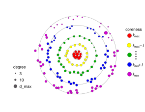
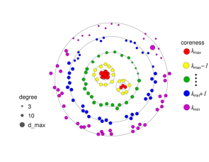
Figure 2: The two drawings show the structure of a typical layout in two important cases: on the left, all $k$-cores are connected; on the right, some $k$-cores are composed by more than one connected component. The vertices are arranged in a series of concentric shells, each one corresponding to a particular $k$-shell. The diameter of the shell depends on both the coreness value and, in case of multiple components (right) also on the relative fraction of vertices belonging to the different components. The color of the vertices corresponds to their coreness value, while their size is logarithmically proportional to their original degree, as shown by the scale going from the minimal to the maximal degree.

4.3 Basic features of the visualization’s layout

The main features of the layout’s structure obtained with the above algorithms are visible in Fig.2 where, for the sake of simplicity, we do not show any edge. The leftmost panel displays the case in which all $k$-cores have a single component, while in the rightmost one an example of $k$-core fragmentation is reported. Indeed, it is possible that, during the pruning procedure, the remaining nodes forming a $k$-core do not belong to the same connected component. When such a fragmentation occurs, the algorithm computes the multiple components of the core and displays all of them in a coherent way.

$\bullet$ The visualization’s layout is two-dimensional, composed of a series of concentric circular shells (see the five different shells in Fig.2).

$\bullet$ Each shell corresponds to a single coreness value and all vertices in it are therefore drawn with the same color. A color scale allows to distinguish different coreness values: in the layouts, as in Fig.2, the violet is used for the minimum value of coreness $k_{min}$, then nuances of blue, green and yellow compose a graduated scale for higher and higher coreness values up to the maximum value $k_{max}$ that is colored in red.

$\bullet$ The diameter of each $k$-shell depends on the coreness value $k$, and is proportional to $k_{max}-k$ (In Fig.2, the position of each shell is identified by a circle having the corresponding diameter). The presence of a trivial order relation in the coreness values ensures that all shells are placed in a concentric arrangement. On the other hand, when a $k$-core is fragmented in two or more components, the diameters of the different components depend also on the relative number of vertices belonging to each of them, i.e. the fraction between the number of vertices belonging to that component and the total number of vertices in that coreness set. This is a very important information, providing a way to distinguish between multiple components at a given coreness value. Looking at the two central components for high coreness values in Fig.2 (right), we immediately realize that the bigger one contains a larger fraction of vertices.

$\bullet$ Finally, the size of each node is proportional to the original degree of that vertex; we use a logarithmic scale for the size of the drawn bullets.

5 Network fingerprinting

The $k$-core decomposition peels the network layer by layer, revealing the structure of the different shells from the outmost one to the more internal ones. The algorithm provides a direct way to distinguish the network’s different hierarchies and structural organization by means of some simple quantities: the radial width of the shells, the presence and size of clusters of vertices in the shells, the correlations between degree and coreness, the distribution of the edges interconnecting vertices of different shells, etc. The following features are useful to extract this structural information out of the visualization. We also highlight the role of the parameters $\epsilon$, $\delta$ and $\gamma$ of the visualization algorithms in helping to determine the structural characteristics of the visualized network.

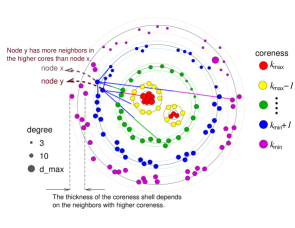
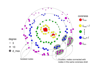
Figure 3: The figure on the left shows that each shell has a certain radial width. This width depends on the correlation’s properties of the vertices in the shell. The dashed lines in the figure point out the width of the outmost shell, that corresponds to the lowest $k$-shell. In the second shell, we have pinpointed two nodes $x$ and $y$. The node $y$ is more internal than $x$ because a larger part of its neighbors belongs to higher $k$-shells compared to $x$’s neighbors. Indeed, $y$ has three links to nodes of higher coreness, while $x$ has only one. The figure on the right shows the clustering properties of nodes in the same $k$-shell. In each $k$-shell, nodes that are directly connected between them (in the original graph) are drawn close one to the other, as in a cluster. Some of these sets of nodes are circled and highlighted in gray. Three examples of isolated nodes are also indicated; these nodes have no connections with the others of the same shell.

1) Shells Width: In the graph representations the width can change considerably from shell to shell. The thickness of a shell depends on the coreness properties of the neighbors of the vertices in the corresponding coreness set. For a given shell-diameter (corresponding to the black circle in the median position of shells in Fig.3), each vertex can be placed more internal or more external with respect to this reference line. Nodes with more neighbors in higher coreness sets are closer to the center and viceversa, as shown in Fig.3. Node $y$ is more internal than node $x$ because it has three edges towards higher coreness nodes compared to the single edge emerging from $x$ towards inner shells. The maximum thickness of the shells is controlled by the $\epsilon$ parameter (Eq. 1).

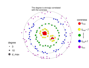
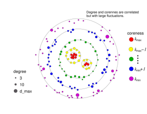
Figure 4: The two figures show different correlation properties between the coreness and the degree of the nodes. On the left, we report a graph with strong degree-coreness correlation: the size of the nodes grows going from the periphery to the center, in strong correlation with the coreness. The right-hand drawing shows a graph in which there is the degree-coreness correlations are blurred by large fluctuations, as stressed by the presence of some hubs in the external shells.

2) Shell Clusters: The angular distribution of vertices in the shells is not completely homogeneous. Fig.3 shows that clusters of vertices can be observed. The idea is that of grouping together all nodes of the same coreness set that are directly linked in the original graph and of representing them close one to another in the shell. Thus, a shell is divided in many angular sectors, each one containing a cluster of vertices. This feature allows to figure out at a glance if the coreness sets are composed of a single large connected component rather than divided into many small clusters, or even if there are isolated vertices (i.e. disconnected from all other nodes in the shell, not from the rest of the $k$-core!).

3) Degree-Coreness Correlation: Another property that can be studied from the obtained layouts is the correlation between the degree of the nodes and the coreness value. In fact, both quantities are centrality measures and the presence or the absence of correlations between them is a very important feature characterizing a network’s topology. The nodes displayed in the most internal shells are those forming the central core of the network; the presence of degree-coreness correlations then corresponds to the fact that the central nodes are most likely high-degree hubs of the network. This effect is indeed observed in many real communication networks with a clear hierarchical structure, as the Internet at the Autonomous System level or the World Wide Air-transportation network. On the contrary, the presence of hubs in external shells is typical of networks without a clear global hierarchical structure as the World-Wide Web or the Internet Router Level. In this case, emerging star-like configurations appear with high degree vertices connected only to very low degree vertices. These vertices are rapidly pruned out in the k-core decomposition even if they have a very high degree, leading to the presence of local hub in the external k-shells, as in Fig. 4.

4) Edges: The visualization shows only a homogeneously randomly sampled fraction of the edges. We can tune the percentage of drawn edges in order to get the better trade-off between the clarity of visualization and the necessity of giving information on the way the nodes are mainly connected. Edge-reduction techniques can be implemented to improve the algorithm’s capacity in representing edges; however, a homogeneous sampling does not alter the extraction of topological information, ensuring a low computational cost. Finally, the two halves of each edge are colored with the color of the corresponding extremities to make more evident the connection among vertices in different shells.

5) Disconnected components: The fragmentation of any given k-shell in two or more disconnected components is represented by the presence of a corresponding number of circular shells with different centers (Fig. 2). The diameter of these circles is related with the number of nodes of each component and modulated by the $\gamma$ parameter (Eq. 7). The distance between components is controlled by the $\delta$ parameter (Eq. 4).

In summary, the proposed algorithm makes possible a direct, visual investigation of a series of properties: hierarchical structures of networks, connectivity and clustering properties inside a given shell; relations and interconnectivity between different levels of the hierarchy, correlations between degree and coreness, i.e. between different measures of centrality.

6 Results from computer-generated and real networks

In the following we provide specific examples in which the use of the proposed visualization algorithm readily allows the identification of characteristic fingerprints and hierarchies in a set of real and computer generated networks. In particular, the visualization allows to identify the lack of hierarchy and structure of the basic Erdös-Rényi random graph. Similarly the time correlations present in the Barabási-Albert network find a clear fingerprint in our visualization layout. A further interesting example is the identification of the different hierarchical arrangement of the Internet network when visualized at the Autonomous system level and the Router level. These examples provide an illustration of the use and capabilities of the proposed algorithm in the analysis of large sparse graphs. The parameters are set to the values $\epsilon=0.18$, $\delta=1.3$ and $\gamma=1.5$, which provide a readable layout at the definition allowed in the present paper format.

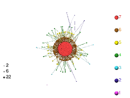
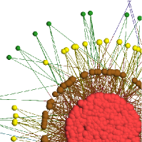
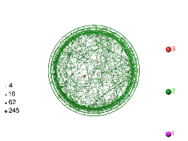
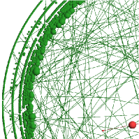
Figure 5: Graphical representation of an ER network with average degree $10$ and 1000 vertices (left) and of a BA network with $m=2$ and $n=10000$ (right).

6.1 Visualization and analysis of computer-generated graphs

In this section we want to provide the visualization of a set of computer generated networks generally used in the literature to model large scale graphs. We will show that the proposed algorithm provides a very intuitive visualization of the difference between the models and the real networks. In this perspective, the $k$-core decomposition appears as a suitable tool in the examination and validation of network models.

The Erdös-Rényi (ER) model [17], with poissonian degree distribution, is a typical example of graphs with a characteristic value for the degree (the average value $\langle d\rangle$). Since an ER graph can consist of more than one connected component, we consider only the largest of these components. An instance of the visualization of Erdös Rényi random graphs is provided by Figure 5: the maximum coreness is clearly related to the average degree $\langle d\rangle=10$. The large central mass is the result of the very homogeneous topology; the vertex degrees have only small fluctuations, thus most vertices belong to the same $k$-core that is also the highest.

Since many real-world networks have been shown to display a very heterogeneous topology as measured by broad degree distributions, many models and mechanisms have been proposed to construct heterogeneous networks. The most famous is the Barabási-Albert (BA) model [18], which considers growing networks according to the preferential attachment mechanism: each new vertex is connected to $m$ already existing vertices chosen with a probability proportional to their starting degree. This model produces graphs with power-law degree distributions, thus characterized by a very large variety of degree values. Such a graph, with $m=2$, shown in Fig. 5 produces a quite peculiar decomposition. Indeed, although this graph displays a very heterogeneous vertex degree distribution, its $k$-core decomposition is trivial; only few layers at very small coreness are visible. The construction mechanism provides a simple explanation. Each new vertex enters the system with degree $m$, but at the following time steps new vertices may connect to it, increasing its degree. Inverting the procedure, we obtain exactly the $k$-core decomposition. The minimum degree is $m$, therefore all coreness sets $C_{c}$ with $c<m$ are empty. Recursively pruning all vertices of degree $m$, one first removes the last vertex, then the one added at the preceding step, whose degree is now reduced to the initial value $m$, and so on, up to the initial vertices which may have larger degree. Hence, all vertices except the initial ones belong to the coreness set of coreness $m$. This somewhat pathological property holds for all growing networks with fixed initial number of links for new vertices. Simple variations of the basic algorithm and the introduction of stochasticity in the growing procedure result in more complicate structures.

6.2 Visualization of real networks

We first present a visualization of a portion of the .fr domain of the World Wide Web (WWW). Its graph is composed by one million pages. This network, whose visualization is presented in Figure 6, is particularly interesting because at the $12$-core level two disconnected components emerge. Note that, since the actual definition of $k$-cores concerns undirected graphs, we consider here the WWW as undirected.

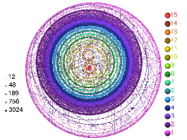
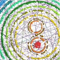
Figure 6: Graphical representation of a fraction of the .fr domain of Web.

We also provide the visualization of networks representing Internet at various granularity levels. More precisely, we consider graphs of Internet at the autonomous system and router level. The autonomous system level is represented by collected routes of Oregon route-views [19] project, called AS, and its extended version AS+ presented in Chen et al. [20], both from May 26, 2001. For the router level, we use the graph obtained by an exploration of Govindan and Tangmunarunkit [21] in 2000, called here IR graph, and the IR_CAIDA graph obtained from the CAIDA project [22] between April 21st and May 8th, 2003. Both networks are composed by approximately $200000$ nodes. The two ASes maps (close to $11500$ nodes each) differ mainly in the number of links: the AS+ maps were constructed by using informations from peering relationship of autonomous systems, obtained from Looking Glass tools. These tools are maintained by ISPs to troubleshoot routing problems.

Figure 7 displays the representation of two different maps of the autonomous system graphs (AS and AS+). All coreness layers are populated, and, any given k-shell, the vertices are distributed on a relatively large range of the radial coordinate, which means that their neighborhoods are variously composed. It is worth noting that the coreness and the degree are very correlated, with a clear hierarchical structure. Links go principally from one coreness set to another, although there are of course also intra-layer links. The hierarchical structure exhibited by our analysis of the autonomous system level is a striking property; for instance, one might exploit it for showing that in the Internet high-degree vertices are naturally (as an implicit result of the self-organizing growth) placed in the innermost structure.

At high resolution, i.e. at the router (IR) level, Internet’s properties are less structured, as shown in Figure 8, in which a completely different scenario emerges: external layers, of lowest coreness, contain vertices with large degree. For instance, in the IR graph we find 20 vertices with degree larger than 100 which have coreness smaller than 6. The correlation between coreness and degree is thus clearly of a very different nature in the maps of Internet obtained at different granularities i.e. routers or autonomous systems.

The lowest $k$-shells, containing vertices that are very external, are displayed as quite broad shells, meaning that the corresponding vertices have neighbors with coreness covering a large range of values. The larger coreness shells are thin rings, which means that the neighbors of the vertices in a given layer have similar coreness.

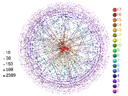
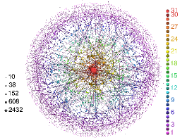
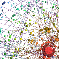
Figure 7: Graphical representation of the AS (left) and AS+ (right) graphs.

It is worth remarking how the present visualization allows the distinction of networks which appear very similar on the basis of the sole statistical properties. Indeed, we can notice that the IR map is quite different from the IR_CAIDA map. This difference likely finds its origin in the different exploration methods used to gather the two data sets. The IR map has been obtained from one source monitor, using source routing to detect lateral connectivity. The IR_CAIDA map, instead, is the merger of data gathered by several different probing monitors. On one hand, it is likely that the most central cores of the IR network are composed by routers with source routing activated (approximately $8\%$ of the total routers [21]). These routers sample destinations unevenly resulting in a less regular layout. On the other hand, the IR_CAIDA map appears to have a very regular structure likely due to a more symmetric exploration process. The obtained layout provides at a glance the evidence for pronounced differences in the structural ordering in the two maps, suggesting the critical examination and comparison of the two experimental strategies.

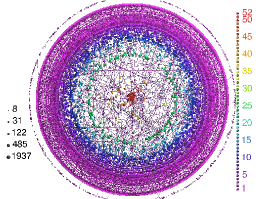
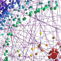
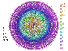
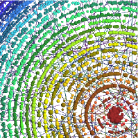
Figure 8: Left: Graphical representation of the IR (left) and IR_CAIDA (right) graphs.

7 Conclusions

In this paper, we have proposed a general visualization tool for large scale graphs. Exploiting $k$-core decomposition, and the natural hierarchical structures emerging from it, our algorithm yields a layout that possesses the simplicity of a 2D representation with a considerable amount of information encoded. One can easily read basic features of the graph (degree, hierarchical structure, position of the highest degree vertices, etc.) as well as more entangled features, e.g. the relation between a vertex and the hierarchical position of its neighbors. Our results show the possibility of gaining clear insights on the architecture of many real world and computer-generated networks by a visualization based on the rationalization of the corresponding graph. In conclusion, the present visualization strategy is a useful tool for a distinction between networks with different topological properties and structural arrangement, but it may be also used for determining if a certain model is in good agreement with real data, providing a further interesting tool for models validation. Finally, we also provide a publicly available tool for visualizing networks [6].

Acknowledgments: We gratefully acknowledge Fabien Mathieu of LIRMM at Montpellier, France, for providing the .fr portion of the WWW graph. This work has been partially funded by the European Commission - Fet Open project COSIN IST-2001-33555 and contract 001907 (DELIS).

References

- [1] R. Albert and A.-L. Barabási, “Statistical mechanics of complex networks,” Rev. Mod. Phys. 74, pp. 47–, 2000.
- [2] L. A. N. Amaral, A. Scala, M. Barthélemy, and H. E. Stanley, “Classes of small world networks,” Proc. Natl. Acad. Sci. (USA) 97, pp. 11149–11152, 2000.
- [3] S. N. Dorogovtsev and J. F. F. Mendes, Evolution of networks: From biological nets to the Internet and WWW, Oxford University Press, 2003.
- [4] R. Pastor-Satorras and A. Vespignani, Evolution and structure of the Internet: A statistical physics approach, Cambridge University Press, 2004.
- [5] V. Batagelj and M. Zaversnik, “Generalized Cores,” CoRR arXiv.org/cs.DS/0202039, 2002.
- [6] LArge NETwork VIsualization tool, “http://xavier.informatics.indiana.edu/lanet-vi/.”
- [7] COSIN: networks visualization, “http://i11www.ilkd.uni-karlsruhe.de/cosin/tools/index.php.”
- [8] V. Batagelj, A. Mrvar, and M. Zaversnik, “Partitioning Approach to Visualization of Large Networks,” in Graph Drawing ’99, Castle Stirin, Czech Republic, LNCS 1731, pp. 90–98, 1999.
- [9] M. Baur, U. Brandes, M. Gaertler, and D. Wagner, “Drawing the AS Graph in 2.5 Dimensions,” in ”12th International Symposium on Graph Drawing, Springer-Verlag editor”, pp. 43–48, 2004.
- [10] U. Brandes and S. Cornelsen, “Visual Ranking of Link Structures,” Journal of Graph Algorithms and Applications 7(2), pp. 181–201, 2003.
- [11] B. Shneiderman, “Why not make interfaces better than 3d reality?,” IEEE Computer Graphics and Applications 23, pp. 12–15, November/December 2003.
- [12] G. D. Bader and C. W. V. Hogue, “An automated method for finding molecular complexes in large protein interaction networks,” BMC Bioinformatics 4(2), 2003.
- [13] M. Altaf-Ul-Amin, K. Nishikata, T. Koma, T. Miyasato, Y. Shinbo, M. Arifuzzaman, C. Wada, M. Maeda, T. Oshima, H. Mori, and S. Kanaya, “Prediction of Protein Functions Based on K-Cores of Protein-Protein Interaction Networks and Amino Acid Sequences,” Genome Informatics 14, pp. 498–499, 2003.
- [14] S. Wuchty and E. Almaas, “Peeling the Yeast protein network,” Proteomics. 2005 Feb;5(2):444-9. 5(2), pp. 444–449, 2005.
- [15] M. Gaertler and M. Patrignani, “Dynamic Analysis of the Autonomous System Graph,” in IPS 2004, International Workshop on Inter-domain Performance and Simulation, Budapest, Hungary, pp. 13–24, 2004.
- [16] V. Batagelj and M. Zaversnik, “An O(m) Algorithm for Cores Decomposition of Networks,” CoRR arXiv.org/cs.DS/0310049, 2003.
- [17] P. Erdös and A. Rényi, “On random graphs I,” Publ. Math. (Debrecen) 6, pp. 290–297, 1959.
- [18] A.-L. Barabási and R. Albert, “Emergence of scaling in random networks,” Science 286, pp. 509–512, 1999.
- [19] University of Oregon Route Views Project. http://www.routeviews.org/.
- [20] Q. Chen, H. Chang, R. Govindan, S. Jamin, S. Shenker, and W. Willinger, “The Origin of Power Laws in Internet Topologies Revisited,” in IEEE Infocom 2002, 2002.
- [21] R. Govindan and H. Tangmunarunkit, “Heuristics for Internet Map Discovery,” in IEEE INFOCOM 2000, pp. 1371–1380, IEEE, (Tel Aviv, Israel), March 2000.
- [22] Cooperative Association for Internet Data Analysis, Router-Level Topology Measurements. http://www.caida.org/tools/measurement/skitter/router_topology/.