Single-solution Random 3-SAT Instances

Abstract

We study a class of random 3-SAT instances having exactly one solution. The properties of this ensemble considerably differ from those of a random 3-SAT ensemble. It is numerically shown that the running time of several complete and stochastic local search algorithms monotonically increases as the clause density is decreased. Therefore, there is no easy-hard-easy pattern of hardness as for standard random 3-SAT ensemble. Furthermore, the running time for short single-solution formulas increases with the problem size much faster than for random 3-SAT formulas from the phase transition region.

1 Introduction

The propositional satisfiability problem is one of the most studied problems in computer science. The most prominent one is the 3-satisfiability (3-SAT) problem. It consists of determining if there exists an assignment of truth values to a set of boolean variables such that a given 3-SAT formula is satisfied. A 3-SAT formula involving $n$ variables is a conjunction (logical AND) of $m$ clauses, each clause being a disjunction (logical OR) of $3$ literals (a literal is a variable or its negation). 3-SAT problem is important from a theoretical as well as from a practical point of view. On the theoretical side, it is a paradigmatic example of a NP-complete (NPC) problem. Historically, it was the first problem to be shown by Cook [1] to be NPC. The algorithmic complexity of 3-SAT problem is connected to various computational complexity issues, most notably to the famous “P=NP?” question which is one of the most important unsolved problems in mathematics and computer science [2]. On the practical side, 3-SAT solving algorithms are used in the industry. Because any circuit involving logical operations can be converted to a 3-SAT formula they can also be used for verification of microprocessors [3, 4]. 3-SAT solving can also be related to deductive reasoning: given a set of facts (statements) $\phi$, a new statement $C$ can be deduced if a union $\phi\cup\{\lnot C\}$ is not satisfiable, i.e. we arrive at the contradiction assuming the negation $\lnot C$.

Having hard  3-SAT instances at hand is important for several reasons. First, it might help in understanding what makes 3-SAT problems, and generally NPC ones, so difficult at all. Second, hard instances are also actively sought for algorithm testing, enabling the design of better algorithms. There are basically two classes of 3-SAT instances used in testing. Those coming from the real world applications mentioned above and artificially generated ones that are thought to be hard. For the later ones one usually uses the so-called uniform random 3-SAT ensemble. An important discovery was that among random 3-SAT instances hard ones are found around the phase transition [5, 6, 7, 8, 9, 10], where the average formula changes from being satisfiable to being unsatisfiable. Connected to the phase transition phenomenon, it is believed that for NPC problems one typically has a pattern of “easy-hard-easy” problem difficulty as some parameter is varied, with the peak difficulty occurring at the phase transition.

If considering single 3-SAT instances one can ask for instance if a given formula is harder than some other one. For NP-completeness the relevant question is how the running time of the hardest instance (for a given $n$) increases with its size. It is important to realize that if we want to talk about perhaps more interesting statistical properties (e.g. scaling of the running time, phase transition etc.) one has to specify an ensemble of 3-SAT instances, that is defining a measure, i.e. a probability do draw some instance. Therefore, a phase transition phenomenon is not an inherent property of 3-SAT problem alone but of the measure, i.e. it is induced by the drawing procedure (for instance for uniform random 3-SAT). But whereas for physical systems there exists a natural measure, there is no such thing for mathematical problem like 3-SAT. Physical systems have a distinguished quantity called the energy which induces the canonical measure. The canonical measure depends on the temperature and as this parameter is varied a phase transition can occur. For 3-SAT problem there is no such “natural” measure. For the most frequently studied random 3-SAT ensemble literals occur in clauses with equal probability. While this might seem a least biased choice there is no a priori reason why such a measure is better than any other. As the random 3-SAT ensemble is just one of many possible ones it is in a way surprising than since the discovery of phase transition in 3-SAT most studies have been concerned with random 3-SAT ensemble (for earlier study of the so-called “random clause length” SAT ensemble see, e.g. [11]). In fact, the measure for random 3-SAT is based on the syntax of the particular encoding of the problem, therefore it is not directly related to the problem structure. It might be useful to consider measure which directly depends on an inherent 3-SAT property, e.g. on the number of satisfying assignments. An interesting question then is how do the properties of an ensemble depend on the chosen measure? One of the initial ideas was [12] that NP-completeness is intimately connected to the phase transition phenomenon. Does one therefore have an easy-hard-easy pattern also for other 3-SAT ensembles? Also, what is the hardness of instances from other ensembles, are they harder than instances from the phase transition for random 3-SAT?

In this work we will try to answer some of these questions. We will study an ensemble of random 3-SAT instances having a single satisfying assignment. By an empirical study of the running time of several complete and incomplete algorithms we are going to show that there is no hardness-peak for this ensemble. In addition, such single-solution instances also seem to be much harder than 3-SAT instances from random 3-SAT phase transition region. We have been actually drawn to 3-SAT problems with one solution while studying quantum adiabatic algorithm for 3-SAT. Quantum adiabatic algorithm  attracted attention because there has been numerical evidence (for small problems) that the running time for random 3-SAT instances from the phase transition region increases only quadratically with the size $n$ [14]. Contrary to that, the scaling of adiabatic algorithm for instances with a single solution seems to be rather exponential [15]. It is therefore also interesting to compare the performance of classical algorithms for these two ensembles, particularly because some stochastic local search algorithms seem to be fairly efficient on random 3-SAT problems from the phase transition. Random instances with a constant number of satisfying assignments could also improve our understanding of phase transition phenomenon in random 3-SAT. Let us first briefly review some known facts about the uniform random 3-SAT ensemble.

2 Uniform Random 3-SAT

A 3-CNF formula is a logical statement involving $n$ boolean variables $b_{i}$. It consists of $m$ clauses $C_{i}$ in conjunction (logical AND $=\land$), $C_{1}\land C_{2}\land\cdots\land C_{m}$, where each clause $C_{i}$ is a disjunction (logical OR $=\lor$) of 3 literals, where a literal is a variable $b_{i}$ or its negation $\lnot b_{i}$ (logical NOT$=\lnot$). 3-SAT problem is to decide whether a given 3-CNF formula, denoted by $\phi$, is satisfiable, i.e. whether there exists a truth assignment of variables $b_{i}$ such that $\phi$ is true. Such prescription is called a solution, the number of which will be denoted by $r$. A given assignment of all variables will be called a state. An instance from a uniform random 3-SAT ensemble is generated by drawing three different random variables for each clause and negating each with probability $\frac{1}{2}$. The number of different clauses is therefore $s=8{n\choose 3}$.

For random 3-SAT problems it has been established that the relevant order parameter for the phase transition is a ratio of the number of clauses and the number of variables, the so-called clause density $\alpha=m/n$ [5, 8, 9]. The critical value $\alpha_{\rm c}\approx 4.25$ for the transition between satisfiability and unsatisfiability coincides with the peak in hardness, i.e. the peak in the running time of an algorithm see, e.g. Figure 4. Below this critical $\alpha_{\rm c}$ random problems are satisfiable with high probability as they are underconstrained, while above it they are unsatisfiable because they are overconstrained. The width of the transition region in parameter $\alpha$ has been shown to decrease as $\sim 1/n^{2/3}$ with the number of variables [7]. Still, we do not have an exact expression for the location of the transition point. The best present proved bounds for the critical $\alpha$ are $3.42$ for satisfiability border [16] and $4.506$ for unsatisfiability border [17], therefore $3.42<\alpha_{\rm c}<4.506$. See the review by [18] for references about the location of the transition point.

A very fruitful approach to 3-SAT problem is to convert it to a spin glass system and then use various powerful statistical methods. One can convert a given 3-SAT formula to a (classical) Hamiltonian by the following simple prescription: for each variable $b_{i}$ a spin variable $S_{i}$ is assigned with the value $S_{i}=1$ corresponding to $b_{i}=1$ and $S_{i}=-1$ for $b_{i}=0$. The Hamiltonian, whose expectation value counts the number of unsatisfied clauses by a state, is a sum of terms for each clause $C_{i}$, $H=\sum_{i=1}^{m}{H_{C_{i}}}$, where the rule for the Hamiltonian $H_{C_{i}}$ describing the clause $C_{i}$ can be best seen from an example, $(b_{2}\lor\lnot b_{4}\lor b_{5})\longrightarrow H_{C_{i}}=\frac{1}{8}(1-S_{2})(1+S_{4})(1-S_{5})$, i. e. the signs in front of spin variables are determined by clauses. A solution will therefore have energy $0$, and the question of satisfiability is translated into the question about the ground state of $H$ with energy zero. Statistical methods have been used to estimate $\alpha_{\rm c}$ and to show that the number of solutions just below the transition point is exponentially large [19], so the transition is reminiscent of a discontinuous (1st order) phase transition in statistical physics. Analysis of the phase space structure also resulted in a new survey propagation algorithm [20]. The hardness of instances at the transition point has been connected with the discontinuous occurrence of a “backbone”. A backbone is a set of variables that are fully constrained, i.e. have the same value in all solutions. Below $\alpha_{\rm c}$ the backbone is zero, while it is nonzero (and bounded away from zero) above $\alpha_{\rm c}$ [21]. If the backbone is large and the problem is overconstrained a backtracking algorithm will quickly “realize” it made a wrong assignment. On the other hand if the backbone is small and the problem is underconstrained there are many “good” beginning assignments which will lead to the solution.

3 Related work

In this section we will give a list of related studies that deal with the subjects covered in the present paper. This includes studies of instances with a fixed number of solutions, scaling of the running time with $n$, generating methods for hard instances and various results about the difficulty of short 3-SAT formulas (having small $m$).

Most of the studies of random 3-SAT ensemble have been concerned with the computational cost at a constant $n$ as a function of the ratio $m/n$, where the characteristic phase transition-like curve is observed. This is in a way surprising because for the computational complexity (and also for practical applications) it is the scaling of running time as the problem size increases which is important, i.e. changing $n$ at fixed $m/n$. Exponential scaling with $n$ has been numerically observed near the critical point [8, 10] for random 3-SAT as well as above it (albeit with a smaller exponent). Recently the scaling with $n$ has been studied and the transition from polynomial to exponential complexity has been observed below $\alpha_{\rm c}$ [22], again for random 3-SAT.

There has been numerical evidence [5, 23, 24] that below $\alpha_{\rm c}$ short instances of 3-SAT as well as of graph coloring [25] can be hard. With respect to the formula size an interesting rigorous result is [26, 27] that an ordered DPLL algorithm needs an exponential time $2^{\Omega(n/\alpha)}$ to find a resolution proof of an unsatisfiable 3-SAT instance. Note that the coefficient of the exponential growth increases with decreasing $\alpha$, i.e. short formulas are harder. For our ensemble of single-solution formulas we will find the same result.

Generating methods for 3-SAT problems having one solution have been devised employing the Latin square problem [28] as well as transforming the factorization to 3-SAT [29]. In both cases the parameter $\alpha$ of the resulting 3-SAT instances grows with the problem size $n$. One can also use the conversion of some other NPC problem to 3-SAT [30]. Hard instances in the underconstrained region can be generated by embedding a smaller unsatisfiable subproblem [31] into a larger instance. Ferromagnetic phase transition in a spin glass has been exploited to generate hard satisfiable 3-SAT instances in the overconstrained region, $m/n>\alpha_{\rm c}$ [32]. Hard instances can also be generated by hiding satisfying assignments [33]. This work has been extended [34] to produce even harder instances, particularly for stochastic local search methods. For instance, the number of necessary Walksat steps grows exponentially as $\propto 2^{0.1n}$ for the hardest instances generated.

As regards the connection between the number of solutions and the formula difficulty there have been several works, but none studied in detail how the time scales if the number of solutions is held fixed. In [35] it has been found that for constraint satisfaction problem the difficulty monotonically increases by decreasing the phase transition parameter. Later it was found [36] that the existence of the peak in hardness can sensitively depend in the ensemble and the algorithm used. Hoos [37] found a correlation between the number of solutions and the problem difficulty, i.e. instances with less solutions tend to be harder for stochastic local search methods, see also [38]. Problems having a small backbone seem to have stronger correlation between the number of solutions and a local search difficulty [39].

4 Random 3-SAT instances with one solution

Although the precise understanding of the phase transition phenomenon in random 3-SAT is still lacking a frequent heuristic explanation for its occurrence (see, e.g. [40]) is the combination of a decreasing number of solutions as $\alpha$ is increased and at the same time increased pruning of the search three, resulting in the maximal complexity for some intermediate $\alpha$. This “explanation” classifies 3-SAT instances according to the number of solutions they have. Therefore, an ensemble of random 3-SAT instances having a constant number of solutions would presumably tell us also something about the phase transition itself. As a second motivation point to choose a single-solution ensemble is the fact that for some applications [29, 28] a single-solution 3-SAT instances might be more “natural” choice than random 3-SAT.

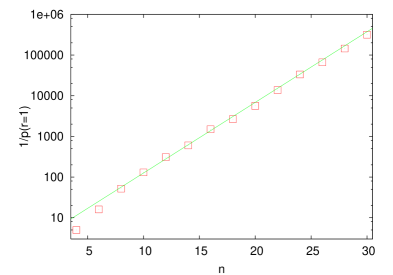
Figure 1: Frequency of 3-SAT formulas with exactly $r=1$ solution among random instances at $m/n=3$, i.e. the inverse probability to get such a formula. Each point is an average over $100$ instances.

Our ensemble therefore consists of random 3-SAT instances that have a single satisfying assignment ($r=1$). As the stress of this paper is to identify a new interesting ensemble of 3-SAT problems and not primarily to generate very large problems, we used a rather inefficient method to generate this ensemble. We obtained random 3-SAT instances with $r=1$ solution by simply filtering randomly generated formulas trough a 3-SAT solver keeping only those with $r=1$. The method is very inefficient because the expected number of solutions (below $\alpha_{\rm c}$) grows exponentially with $n$. Thereby, the probability to find an instance with only one solution among random 3-SAT ensemble decays exponentially with $n$. This can be seen in Figure 1. This rather technical issue of inefficient generation limited us to problems of relatively small size $n\leq 40$. For instance, to generate $1000$ random 3-SAT instances with $n=40$, $r=1$ and $m/n=3$ we had to solve approximately $10^{10}$ randomly generated problems. Still, we think that it is conceivable to generate single-solution problems with constant $\alpha$ in a more efficient way, e.g. by converting one of the many known NPC problems [41] to 3-SAT with one solution. The probability to find single-solution formulas among random 3-SAT instances changes with $m/n$ and attains its maximum at the location of the transition point for random 3-SAT, see Figure 2.

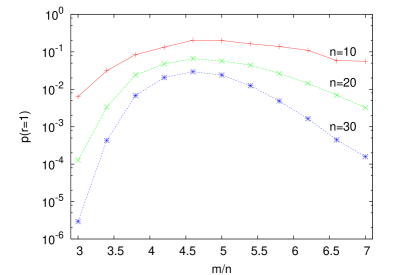
Figure 2: The dependence of probability $p(r=1)$ to find single-solution instance among random 3-SAT ensemble for three different $n$.

4.1 Algorithms used

We will test several algorithms for solving 3-SAT problem. Generally there are two classes of algorithms : (i) a complete ones that determine satisfiability or unsatisfiability of a given formula. They terminate after a finite number of steps, either by finding a solution or proving unsatisfiability. (ii) incomplete algorithms which can only find a solution but can not prove unsatisfiability. In principle they have no terminating condition and can therefore be used only on satisfiable formulas on which though they can perform better than complete algorithms. Typically they employ some sort of a localized random search.

The most popular complete method is the DPLL algorithm [42], sometimes called also just DP algorithm because it is based on an earlier algorithm by Davis and Puttnam [43]. DPLL is a backtracking depth-first algorithm. It assigns truth values to variables and simplifies the formula. The simplification of formula $\phi$ when assigning TRUE value to a single literal $v$ consists of deleting clauses that are satisfied by the truth assignment, i.e. contain literal $v$, and deleting all literals contradicting the assignment in other clauses, i.e. all occurrences of $\lnot v$. The algorithm therefore descends along the state tree by recursive calls until it either finds a solution or encounters a contradiction, i.e. an empty clause occurs. In the later case it backtracks by changing a previously made assignment. The number of recursive calls of DPLL procedure is a good measure of running time. There are different variants of DPLL algorithm depending on the variable-selection rule, i.e. on the heuristics how we choose the next variable whose value we assign. In the algorithm we use we pick the first variable in the first unsatisfied clause.

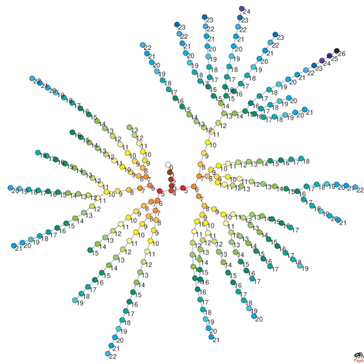
Figure 3: Search tree of the DPLL algorithm for 3-SAT instance with $n=26$ and $m/n=3$ having one solution, $r=1$. Color of vertices and numbers denote the number of assigned variables.

To illustrate DPLL algorithm we can plot a search tree as shown in Figure 3 for an instance with $n=26$ variables and $m/n=3$, having exactly one solution, $r=1$. Each vertex denotes a state with a certain number of assigned variables, the number of which is printed next to a vertex. The algorithm therefore starts from the white vertex with the number $0$ and ends at the black vertex with the number $26$, denoting a state which is a solution of 3-SAT formula. The number of DPLL calls needed to find the solution, equal to the number of vertices, was $278$ in this case. The search tree has been plotted using the network analysis program “Pajek” [44].

Nowadays there are of course many modern algorithms that are much faster than the original DPLL one although most of them is still based on DPLL idea. Each year a competition for SAT solvers is organized comparing their performance on artificial and industrial SAT problems [45]. In addition to simple DPLL we have tested also one of those, namely SATO  by H. Zhang [46]. SATO is based on DPLL but uses different splitting rule and also uses “intelligent backjumping”, meaning that it must not backtrack step by step but can jump over several steps. In all numerical experiments the results for SATO were qualitatively the same as for DPLL.

For satisfiable problems the so-called stochastic local search algorithms can be more effective than complete algorithms. We have used GWSAT [47] as our main stochastic algorithm. It is based on GSAT [6, 48], and is one of the most widely studied incomplete methods. At the beginning of the algorithm we randomly draw a state, i.e. choose a random assignment of variables. Then at each step we change the truth value of one variable (such a step is also called a flip). For local search methods we need a cost function that will measure how good different flips are, so that we can choose the best one at each step. In GWSAT we choose with probability $1-p$ the variable to flip as the one which leads to the state with the largest number of satisfied clauses (GSAT step), and with probability $p$ a random variable from a randomly chosen unsatisfied clause. This is repeated until a solution is found. A good measure of running time is the number of flips made until a solution is found. In addition to GWSAT we also tested Walksat [47] and Adaptive Novelty+ [49]. For all stochastic local search algorithm implementations we used the Ubcsat program [50]. Again, as for complete methods, the results for more advanced Walksat and Adaptive Novelty+ algorithms were qualitatively the same as for GWSAT. For a detailed comparison of different local search algorithms see, e.g. [51]

In the next two subsections we will present the main results of the paper, the analysis of the running time of various 3-SAT solving algorithms for an ensemble of random 3-SAT instances with $1$ solution. First we will show the dependence of running time on $\alpha$ at constant $n$ in order to demonstrate that there is no phase transition-like peak in the difficulty.

4.2 Running time at constant $n$

The data for DPLL are shown in Figure 4. In addition to the curve for random instances with $r=1$ we also plot one for random 3-SAT ensemble (arbitrary $r$) and for random instances with $r\geq 1$ solutions. We can clearly see that the running time of instances with exactly one solution increases with decreasing $m/n$ and gets in fact larger for sufficiently small clause density than for instances around the phase transition point for random 3-SAT. The same quantitative results are obtained also for SATO.

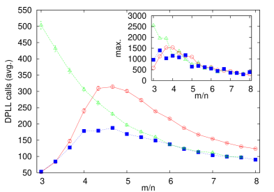
Figure 4: Running time for DPLL algorithm for random 3-SAT with $r=1$ solution (empty triangles), $r\geq 1$ solution (full squares) and arbitrary $r$ (empty circles). In the inset is shown the maximal running time (same three data sets) out of $1000$ instances used for each point. All is for $n=30$.

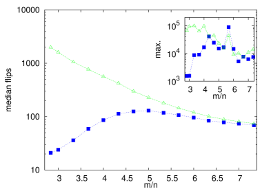
Figure 5: Median running time for GWSAT algorithm for random 3-SAT with $r=1$ solution (empty triangles) and $r\geq 1$ solution (full squares). In the inset is shown the maximal running time (same data sets) out of $1000$ instances used for each point. All is for $n=30$.

In Figure 5 we show the results for GWSAT algorithm. Again one can observe that the running time is larger for single-solution ensemble and that there is no peak in the difficulty. Similar figure is obtained also for Walksat and Adaptive Novelty+. Therefore, one can see that for an ensemble of single-solution random 3-SAT the difficulty monotonically increases with decreasing $m/n$. In comparison to random 3-SAT ensemble there is no peak in the difficulty for our ensemble. In view of that we will in the next section study how the difficulty scales with $n$ for constant $m/n$. Because instances with smaller $m$ are harder, we will choose $m/n=3$. Note that by choosing even smaller $m/n$ one will get even harder instances, but then our inefficient generating method gets too slow.

4.3 Running time at constant $m/n$

Even though one can see in Figures 4 and 5 than instances from single-solution ensemble at $m/n=3$ are harder than the phase transition ones from random 3-SAT ensemble for the shown $n=30$, their difficulty could scale differently with $n$. The real question then is, what happens when we increase $n$.

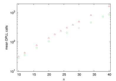
Figure 6: Scaling of the running time for DPLL algorithm. Triangles are for $r=1$ at $m/n=3$ and circles for arbitrary $r$ at $m/n=4.5$.

We will always compare results of a single-solution ensemble at $m/n=3$ and random 3-SAT ensemble at $m/n=4.5$ which is the approximate location of the transition point for random 3-SAT and small $n$ studied here. Each time we will average over 1000 3-SAT instances. In Figure 6 for DPLL algorithm one can see that the running time for single-solution instances increases faster than for random instances from the phase transition point. The difference in hardness therefore increases with increasing size.

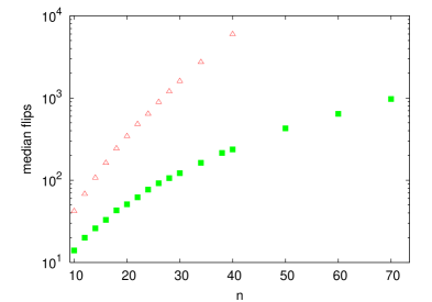
Figure 7: Scaling of the running time for GWSAT algorithm. Empty triangles are for $r=1$ at $m/n=3$ and full squares for $r\geq 1$ at $m/n=4.5$.

Similar results can be observed also for GWSAT in Figure 7. For stochastic search methods we average again over $1000$ instances and for each instance over $100$ runs of the algorithm. The difference again increases with increasing $n$, this time even faster as for DPLL. In Figure 8 we show similar result also for Adaptive Novelty+. The number of necessary flips is smaller as for GWSAT but the overall behavior is qualitatively the same. Although the range of $n$ is relatively small we also plotted the best fitting exponential or power-law dependences. While for random 3-SAT instances from the phase transition one has a slow polynomial $\propto n^{2.0}$ growth of the running time, the increase is much faster, agreeing well with an exponential $\propto 2^{0.18n}$, for single-solution ensemble. The coefficient of exponential growth $0.18$ is actually fairly large, meaning that short single-solution random instances get harder very quickly. For instance, for hard soluble 3-SAT instances reported in [34] the increase of the number of flips for Walksat algorithm was approximately $\propto 2^{0.1n}$ (with a large pre-factor). For our single-solution ensemble Walksat algorithm is slightly slower than Adaptive Novelty+. Interestingly, the same difference between the complexity scaling of two ensembles as here, namely polynomial vs. exponential, has been found also for quantum adiabatic algorithm [14, 15]. It might well be that the instances from the phase transition region of random 3-SAT ensemble are not that difficult and a polynomial average cost algorithm is possible.

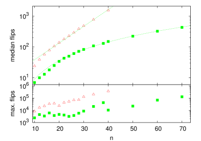
Figure 8: Scaling of the running time for Adaptive Novelty+. Empty triangles are for $r=1$ at $m/n=3$ and full squares for $r\geq 1$ at $m/n=4.5$. Dashed curves are $11\cdot 2^{0.18n}$ (top) and $0.09\cdot n^{2.0}$ (lower). In the lower plot we show the maximal times.

What is the explanation for the difficulty of single-solution random 3-SAT instances with small $m/n$? We will give some heuristic arguments why it might not be so unexpected that such 3-SAT instances are hard to solve.

For single-solution instances it turns out [15] that the number of assignments that violate only one clause, called the excited states, is very large. In fact the number of such excited states grows exponentially with $n$. Therefore, 3-SAT instances from single-solution random ensemble have only one solution and at the same time exponentially many assignments violating only one (or a few) clause. Any complete method, like DPLL for instance, must do exhaustive search in the state tree until a contradiction is encountered and the algorithm has to backtrack. If assignments made are such that we are descending towards an excited state which violates only one clause, a contradiction will occur only after we make an assignment of all three variables occurring in this clause. This can possibly occur very deep within the tree, causing large amounts of backtracking. Simply said, the excited states “fake” the algorithm into descending along the wrong branches. This can be seen in Figure 9. This time the numbers next to vertices denote the number of excited states in the sub-tree below the vertex. We can see, that long branches are usually correlated with a large number of excited states. As a consequence, the search tree is large with many long branches. One can argue also differently: assuming a random truth assignment of the first assigned variable in a DPLL-like algorithm, one will with probability $\frac{1}{2}$ end up with an unsatisfiable problem. For this unsatisfiable problem a rigorous statement [52] about the exponential complexity of DPLL even below the satisfiability border $\alpha_{\rm c}$ suggest an exponential complexity. Similarly, the running time is expected to be exponential also for incomplete stochastic local search methods. For such algorithms the exponential number of excited states will effectively shadow out the single real solution (searching for a needle in a haystack). To circumvent the exponential complexity the algorithm would have to efficiently distinguish between an exponentially many states violating only one clause and a single solution satisfying all clauses. This can not of course be excluded for some yet to be found smart choice of moves or a smart variable-selection rule in a DPLL-like algorithm, but it seems unlikely because there is simply very few information available which the algorithm could use in its heuristics. Remember that we are concentrating on underconstrained instances having as few clauses as possible. Of course, the explanation with excited states is probably only part of the story. It would be interesting to investigate the phase space structure of such instances in greater detail.

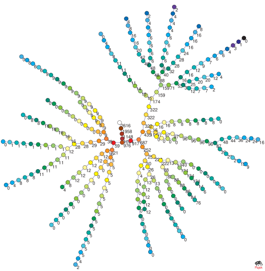
Figure 9: Search tree for DPLL and 3-SAT instance with $n=26$ and $m/n=3$ (the same instance as in Figure 3). Numbers next to vertices denote the number of excited states in the sub-tree below a given vertex. The color of vertices denotes the depth in the tree as before.

5 Conclusions

We have identified and studied a new ensemble of 3-SAT instances, namely random 3-SAT formulae having a single satisfying assignment. Numerical experiments show that the properties of this ensemble are significantly different from those of random 3-SAT ensemble. The difficulty of single-solution instances monotonically increases with decreasing clause density, that is shorter formulas are generally harder. Therefore, this ensemble does not exhibit easy-hard-easy pattern of difficulty. Short single-solution instances (having e.g. $m/n=3$) are in fact much harder than problems from the phase transition region of random 3-SAT ensemble. It would be interesting to investigate the nature of their hardness more in detail. 3-SAT instances can be divided into ensembles according to the number of satisfying assignments they have. Here we studied only the ensemble having one satisfying assignment. An interesting question is, is the behavior of other ensembles similar, for instance that the difficulty of instances decays monotonically with $m/n$? If yes, the occurrence of the maximal difficulty for random 3-SAT at the phase transition can be viewed as being due to the changing of the probability to draw instances with fixed number of solutions. For single-solution instances studied in the present paper, the highest probability to find them among random 3-SAT instances occurs at the transition point and decays fast away from it. Becouse this decay is faster than the increase of their difficulty for small $m$, a maximum of difficulty occurs at the location of the maximum probability.

The author would like to thank the Alexander von Humboldt Foundation for its support.

References

- [1] S. A. Cook, The complexity of theorem-proving procedures, in: Proceedings of the Third IEEE Symposium on the Foundations of Computer Science, 1971, pp. 151–158.
- [2] S. A. Cook, The P versus NP problem, Millenium Problems, Clay Mathematics Institute, http://www.claymath.org/millennium (2000).
- [3] M. Velev, R. Bryant, Effective use of boolean satisfiability procedures in the formal verification of superscalar and VLIW microprocessors, in: Proceedings of the 38th Design Automation Conference (DAC ’01), 2001, pp. 226–231.
- [4] P. Bjesse, T. Leonard, A. Mokkedem, Finding bugs in an alpha microprocessor using satisfiability solvers, in: 13th Conference on Computer-Aided Verification (CAV01), 2001, pp. 454–464.
- [5] D. Mitchell, B. Selman, H. Levesque, Hard and easy distribution of SAT problems, in: Proceedings of the Tenth National Conference on Artificial Intelligence (AAAI’92), 1992, pp. 440–446.
- [6] B. Selman, H. Levesque, D. Mitchell, A new method for solving hard satisfiability problems, in: Proceedings of the Tenth National Conference on Artificial Intelligence (AAAI’92), 1992, pp. 459–465.
- [7] S. Kirkpatrick, B. Selman, Critical behavior in the satisfiability of random boolean expressions, Science 264 (1994) 1297–1301.
- [8] J. M. Crawford, L. D. Auton, Experimental results on the crossover point in satisfiability problems, in: Proceedings of the Eleventh National Conference on Artificial Intelligence (AAAI’93), 1993, pp. 21–27.
- [9] B. Selman, D. Mitchell, H. Levesque, Generating hard satisfiability problems, Artificial Intelligence 81 (1996) 17–29.
- [10] J. M. Crawford, L. D. Auton, Experimental results on the crossover point in random 3-SAT, Artificial Intelligence 81 (1996) 31–57.
- [11] A. Goldberg, On the complexity of the satisfiability problem, Tech. Rep. Courant Computer Science Report No.16., New York University (1979).
- [12] P. Cheeseman, B. Kanefsky, W. M. Taylor, Where the really hard problems are, in: J. Mylopoulos, R. Reiter (Eds.), Proceedings of the Twelfth International Joint Conference on Artificial Intelligence (IJCAI’91), 1991, pp. 331–337.
- [13] P. W. Shor, Progress in quantum algorithms, Quantum Information Processing 3 (2004) 5–13.
- [14] E. Farhi, J. Goldstone, S. Gutman, J. Lapan, A. Lundgren, D. Preda, A quantum adiabatic evolution algorithm applied to random instances of a NP-complete problem, Science 292 (2001) 472–476.
- [15] M. Žnidarič, Scaling of the running time of the quantum adiabatic algorithm for propositional satisfiability, Phys. Rev. A 71 (2005) 062305.
- [16] A. C. Kaporis, L. M. Kirousis, E. G. Lalas, The probabilistic analysis of a greedy satisfiability algorithm, in: R. Möhring, R. Raman (Eds.), Proceedings of the 10th European Symposium on Algorithms (ESA 2002), Vol. 2461 of Lecture Notes in Computer Science, Springer, 2002, pp. 574–585.
- [17] O. Dubois, Y. Boufkhad, J. Mandler, Typical random 3-SAT formulae and the satisfiability threshold, Electronic Colloquium on Computational Complexity (ECCC) 10 (7).
- [18] S. A. Cook, D. G. Mitchell, Finding hard instances of the satisfiability problem: A survey, in: Du, Gu, Pardalos (Eds.), Satisfiability Problem: Theory and Applications, Vol. 35 of Dimacs Series in Discrete Mathematics and Theoretical Computer Science, American Mathematical Society, 1997, pp. 1–17.
- [19] R. Monasson, R. Zecchina, Entropy of the K-satisfiability problem, Phys. Rev. Lett. 76 (1996) 3881–3885.
- [20] M. Mezard, R. Zecchina, Random K-satisfiability problem: From an analytic solution to an efficient algorithm, Phys. Rev. E 66 (2002) 056126.
- [21] R. Monasson, R. Zecchina, S. Kirkpatrick, B. Selman, L. Troyansky, Determining computational complexity from characteristic ’phase transitions’, Nature 400 (1999) 133–137.
- [22] C. Coarfa, D. D. Demopoulos, A. San Miguel Aguirre, D. Subramanian, M. Vardi, Random 3-SAT: The plot thickness, Constraints 8 (2003) 243–261.
- [23] I. Gent, T. Walsh, Easy problems are sometimes hard, Artificial Intelligence 70 (1994) 335–345.
- [24] I. Gent, T. Walsh, The satisfiability constraint gap, Artificial Intelligence 81 (1996) 59–80.
- [25] T. Hogg, C. P. Williams, The hardest constraint problems: A double phase transition, Artificial Intelligence 69 (1994) 359–377.
- [26] P. Beame, R. M. Karp, T. Pitassi, M. E. Saks, On the complexity of unsatisfiability proofs for random k-CNF formulas, in: 30th ACM Symposium on Theory of Computing, 1998, pp. 561–571.
- [27] P. Beame, R. M. Karp, T. Pitassi, M. E. Saks, The efficiency of resolution and Davis-Putnam procedures, SIAM Journal on Computing 31(4) (2002) 1048–1075.
- [28] D. Achlioptas, C. Gomes, H. Kautz, B. Selman, Generating satisfiable instances, in: Proceedings of the Seventeenth National Conference on Artificial Intelligence (AAAI-00), 2000.
- [29] A. Horie, O. Watanabe, Hard instance generation for SAT, in: Proceedings of 8th International Symposium on Algorithms and Computation, Lecture Notes in Computer Science 1350, 1996, pp. 22–31, home page http://www.is.titech.ac.jp/ watanabe/gensat/.
- [30] M. Cadoli, A. Schaerf, Compiling problem specifications into SAT, Artificial Intelligence 162 (2005) 89–120.
- [31] R. J. J. Bayardo, R. C. Schrag, Using CSP look-back techniques to solve exceptionally hard SAT instances, in: Proceedings of the Second International Conference on Principles and Practice of Constraint Programming, Lecture Notes in Computer Science 1118, Springer, 1996, pp. 46–60.
- [32] W. Barthel, A. K. Hartmann, M. Leone, F. Ricci-Tersenghi, M. Weigt, R. Zecchina, Hiding solutions in random satisfiability problems: A statistical mechanics approach, Phys.Rev. Lett. 88 (2002) 188701.
- [33] D. Achlioptas, H. Jia, C. Moore, Hiding satisfying assignments: Two are better than one, preprint cs.ai/0503046 (2005).
- [34] H. Jia, C. Moore, D. Stain, Generating hard satisfiable formulas by hiding solutions deceptively, preprint cs.ai/0503044 (2005).
- [35] B. M. Smith, M. E. Dyer, Locating the phase transition in binary constraint satisfaction problems, Artificial Intelligence 81 (1996) 155.
- [36] D. L. Mammen, T. Hogg, A new look at the easy-hard-easy pattern of combinatorial search difficulty, Journal of Artificial Intelligence Research 7 (1997) 47–66.
- [37] H. H. Hoos, Stochastic local search - methods, models, applications, Ph.D. thesis, TU Darmstadt (1998).
- [38] D. Clark, J. Frank, I. Gent, E. MacIntyre, N. Tomov, T. Walsh, Local search and the number of solutions, in: Proceedings of the Second International Conference on the Principles and Practices of Contraint Programming, Springer, 1996, pp. 119–133.
- [39] J. Singer, I. P. Gent, A. Smaill, Backbone fragility and the local search cost peak, Journal of Artificial Intelligence Research 12 (2000) 235–270.
- [40] C. Williams, T. Hogg, Exploiting the deep structure of constraint problems, Artificial Intelligence 70 (1994) 73–117.
- [41] M. R. Garey, D. S. Johnson, Computers and Intractability: A Guide to the Theory of NP-Completeness, Freeman, 1979.
- [42] M. Davis, G. Logemann, D. Loveland, A machine programm for theorem proving, Communications of the ACM 5 (1962) 394–397.
- [43] M. Davis, H. Putnam, A computing procedure for quantification theory, Journal of the ACM 7 (1960) 201–215.
- [44] V. Batagelj, A. Mrvar, Pajek - analysis and visualization of large networks, in: M. Jünger, P. Mutzel (Eds.), Graph Drawing Software, (series Mathematics and Visualization), Springer, Berlin, 2003, pp. 77–103, home page http://vlado.fmf.uni-lj.si/pub/networks/pajek/.
- [45] D. L. Berre, L. Simon, SAT competition, see web page http://www.satcompetition.org.
- [46] H. Zhang, SATO : An efficient propositional prover, in: Proceedings of International Conference on Automated Deduction (CADE-97), 1997, pp. 272–275, home page http://www.cs.uiowa.edu/ hzhang/sato.html.
- [47] B. Selman, H. A. Kautz, B. Cohen, Noise strategies for improving local search, in: Proceedings of the Twelfth National Conference on Artificial Intelligence (AAAI’94), Seattle, 1994, pp. 337–343.
- [48] B. Selman, H. A. Kautz, Domain-independant extensions to GSAT : Solving large structured variables, in: Proceedings of the Thirteenth International Joint Conference on Artificial Intelligence (IJCAI’93), 1993, pp. 290–295.
- [49] H. H. Hoos, An adaptive noise mechanism for WalkSat, in: Proc. of the 18th Nat’l. Conf. in Artificial Intelligence (AAAI-02), 2002, pp. 665–660.
- [50] D. A. D. Tompkins, H. H. Hoos, UBCSAT: An implementation and experimentation environment for SLS algorithms for SAT and MAX-SAT, in: Proceedings of the Seventh International Conference on Theory and Applications of Satisfiability Testing (SAT 2004), 2004, pp. 305–319.
- [51] H. H. Hoos, T. Stützle, Local search algorithms for SAT: An empirical evaluation, Journal of Automated Reasoning 24 (2000) 421–481.
- [52] D. Achlioptas, P. Beame, M. Molloy, A sharp threshold in proof complexity yields lower bounds for satisfiability search, Journal of Computer and System Sciences 68 (2004) 238–268.