On Optimality Condition of Complex Systems: Computational Evidence

Abstract

A general condition determining the optimal performance of a complex system has not yet been found and the possibility of its existence is unknown. To contribute in this direction, an optimization algorithm as a complex system is presented. The performance of the algorithm for any problem is controlled as a convex function with a single optimum. To characterize the performance optimums, certain quantities of the algorithm and the problem are suggested and interpreted as their complexities. An optimality condition of the algorithm is computationally found: if the algorithm shows its best performance for a problem, then the complexity of the algorithm is in a linear relationship with the complexity of the problem. The optimality condition provides a new perspective to the subject by recognizing that the relationship between certain quantities of the complex system and the problem may determine the optimal performance.

The efficient management of complex systems is increasingly important. However, despite significant progress and interest in complex systems Holland_1 , there is a limited understanding of the problem. In particular, because the existence of principles governing the non-equilibrium situation has not yet been established Ball_1 , the possibility of a general condition determining the optimal performance of a complex system is still unknown. We aim to contribute in this direction and present results of computational experiments in order to discuss the possibility of an optimality condition of complex systems. The results provide a new perspective to the subject by recognizing that the relationship between certain quantities of the complex system and the problem may determine the optimal performance.

In this Letter, we consider an optimization algorithm as a complex system by using the benchmark traveling salesman problems Reinelt_1 . For any problem tested, we can control the performance of the algorithm as a convex function with a single optimum. Consequently, we take this opportunity to investigate whether the performance optimums may be characterized in terms of an optimality condition of the algorithm. Namely, we describe the algorithm by a trace of the variance-covariance matrix derived from the dynamics of the algorithm as a complex system. We also specify a problem by a trace of the distance matrix. Remarkably, the computational analysis of the performance optimums reveals a relationship between the quantities of the algorithm and the problem by approximating it well enough with a linear function.

To recognize the potential importance of the result, we interpret the quantities as the complexities of the algorithm and the problem, and formulate the following optimality condition: if the algorithm shows its best performance for a problem, then the complexity of the algorithm is in the linear relationship with the complexity of the problem. Further experimental facts suggest how the optimality condition may be extended into a wider context.

Let us consider an optimization algorithm ${\cal A}$ as a complex system of $N$ computational agents that minimize the average distance in the traveling salesman problem. All agents start in the same city and at each step an agent visits the next city by using one of two strategies: a random strategy, i.e., visit the next city at random, or the greedy strategy, i.e, visit the next closest city. We define that all agents start with the random strategy. The state of the agents visiting $n$ cities of the problem can be described at step $j=1,...,n-1$ by a binary sequence $s_{j}=s_{1j}...s_{Nj}$, where $s_{ij}=+1$, if agent $i=1,...,N$ uses the random strategy and $s_{ij}=-1$, if the agent uses the greedy strategy to visit the next city. The dynamics of the agents is realized through their choice of strategies and can be encoded by an $N\times(n-1)$ binary strategy matrix $S=\{s_{ij},\ i=1,...,N,\ j=1,...,n-1\}$.

We introduce a variable parameter $v$ that controls the dynamics of the agents in a specific manner. Let $D_{ij}$ be the distance travelled by agent $i=1,...,N$ after $j=1,...,n-1$ steps and

$$D_{j}^{-}=\min_{i=1,...,N}D_{ij},\ D_{j}^{+}=\max_{i=1,...,N}D_{ij}.$$

All distances travelled by the agents after $j=1,...,n-1$ steps belong to the interval $[D_{j}^{-},D_{j}^{+}]$. The parameter $v$ specifies a threshold point

$$D_{j}(v)=D_{j}^{+}-v(D_{j}^{+}-D_{j}^{-}),\ \ \ 0\leq v\leq 1+\gamma,\ \ \ \gamma=0.1$$

dividing the interval into two parts, i.e., successful $[D_{j}^{-},D_{j}(v)]$ and unsuccessful $(D_{j}(v),D_{j}^{+}]$. If the distance $D_{ij}$ travelled by agent $i=1,...,N$ after $j=1,...,n-1$ steps belongs to the successful interval, then we regard the agent’s last strategy as successful. If the distance $D_{ij}$ belongs to the unsuccessful interval, then the agent’s last strategy is unsuccessful.

In order to choose the next strategy, each agent uses an optimal rule Korotkikh_1 that relies on the Prouhet-Thue-Morse (PTM) sequence and has the following description:

1. If your last strategy is successful, continue with the same strategy.

2. If your last strategy is unsuccessful, consult PTM generator which strategy to use next.

The PTM sequence $+1-1-1+1-1+1+1-1\ ...\$ gives a symbolic description of chaos resulting from period-doubling Feigenbaum_1 in complex systems Allouche_1 . It can be also associated with formation processes of integer relations progressing well through the levels of a hierarchical structure Korotkikh_1 . The formation processes produce a measure of complexity Korotkikh_1 that we use as a guide in defining the complexities of the algorithm and the problem.

Each agent has its own PTM generator and a pointer attached to it. The pointer starts with the first bit of the PTM sequence and after each consultation moves one step further, so that the next bit of the PTM sequence can be used, if the strategy is unsuccessful. The control is realized by changing the parameter $v$ from $0$ to $1+\gamma$. For the limiting values of the parameter $v$, the algorithm ${\cal A}$ produces the following dynamics of the agents.

When $v=0$, then $D_{j}(v)=D_{j}^{+}$. Therefore, the successful interval $[D_{j}^{-},D_{j}(v)]$ coincides with the whole interval $[D_{j}^{-},D_{j}^{+}]$ and the last strategy of each agent is successful at each step $j=1,...,n-1$. This means that each agent always uses the random strategy and the strategy matrix becomes

$$S=\left(\begin{array}[]{ccccc}+1&+1&...&+1&+1\\ +1&+1&...&+1&+1\\ .&.&...&.&.\\ +1&+1&...&+1&+1\\ +1&+1&...&+1&+1\\ \end{array}\right)$$

In the opposite limit, when $v=1+\gamma$, then $D_{j}(v)<D_{j}^{-}$. Thus, the unsuccessful interval $(D_{j}(v),D_{j}^{+}]$ covers the whole interval $[D_{j}^{-},D_{j}^{+}]$. This means that the last strategy of each agent is always unsuccessful and, according to the rule, at each step $j=1,...,n-1$ an agent asks the PTM generator which strategy to use next. As a result, the binary sequence of each agent becomes the initial segment of length $(n-1)$ of the PTM sequence and the strategy matrix is turned to

$$S=\left(\begin{array}[]{ccccc}+1&-1&...&-1&+1\\ +1&-1&...&-1&+1\\ .&.&...&.&.\\ +1&-1&...&-1&+1\\ +1&-1&...&-1&+1\\ \end{array}\right)$$

The role of the parameter $v$ may be seen in terms of correlations. When $v=0$, the agents are independent, because the behavior of an agent does not depend on the others. However, as the parameter $v$ gets larger, the successful interval gets smaller, and the behaviors of the agents become more correlated through the PTM sequence. To stay independent, an agent has to show a result approaching the current minimum. Consequently, the rule urges an agent to follow the PTM sequence more strongly and as a result, the presence of the PTM sequence in the strategy matrix becomes more evident. When $v=1+\gamma$, the whole strategy matrix consists of the PTM sequences.

By extensive computational experiments, we investigate how the performance of the algorithm ${\cal A}$ may depend on the parameter $v$. We tested the problems $P$ = $\{$eil76, eil101, st70, rat195, lin105, kroC100, kroB100, kroA100, kroD100, d198, kroA150, pr107, u159, pr144, pr144, pr152, pr226, pr136, pr76, ts225$\}$ belonging to the benchmark traveling salesman problems Reinelt_1 . Let $D_{i}(p,v)$ be the distance travelled by agent $i=1,...,N$ for a problem $p\in P$ and a value $v$ of the parameter. The performance of the algorithm ${\cal A}$ is characterized by the average distance travelled by $N$ agents $D(p,v)=\sum_{i=1}^{N}D_{i}(p,v)/N$, which is sought to be minimized.

In the experiments, the algorithm ${\cal A}$ is applied to each problem $p\in P$ with the number of agents $N=2000$ and values $v_{i}=i\triangle v,\ i=0,1,...,20,\ v=1.1$ of the parameter, where $\triangle v=0.05$. To eliminate randomness, the computations are repeated in a series of $10$ tests and the performance functions $\{D_{k}(p,v),\ k=1,...,10\}$ are averaged into $\bar{D}(p,v)$. Remarkably, for each problem $p\in P$, it is found that the performance $\bar{D}(p,v)$ of the optimization algorithm ${\cal A}$ behaves as a convex function of the parameter $v$ with the only optimum at $v^{*}(p)$ (Fig. 1).

Figure 1: The performance of the algorithm ${\cal A}$ as a convex function of the parameter $v$ for problem ei101.

We characterize the performance optimums $\{v^{*}(p),\ p\in P\}$ by certain quantities of the algorithm and the problem and interpret the quantities as their complexities. The algorithm ${\cal A}$ is described by the quadratic trace of the variance-covariance matrix derived from the strategy matrix Korotkikh_2 . Namely, for a problem $p\in P$, a set of strategy matrices $S_{k}(v^{*}(p))=\{s_{ij}(k),i=1,...,N;\ j=1,...,n-1\},k=1,...,10$ is obtained as a result of ten runs for the value $v^{*}(p)$ of the parameter. For each strategy matrix $S_{k}(v^{*}(p)),k=1,...,10$ the variance-covariance matrix $V(S_{k}(v^{*}(p)))=\{V_{ij}(k),\ i,j=1,...,N\},i=1,...,10,$ and its quadratic trace

$$tr(V^{2}(S_{k}(v^{*}(p))))=\sum_{i=1}^{N}\lambda_{ik}^{2}$$

are computed, where $V_{ij}(k)$ is the linear correlation coefficient between agents $i=1,...,N$ and $j=1,...,N$ and $\lambda_{ik},i=1,...,N,\ k=1,...,10$ are the eigenvalues of the variance-covariance matrix $V(S_{k}(v^{*}(p)))$.

The average $tr(V^{2}(S(v^{*}(p))))$ of the traces is used to describe the complexity

$$C({\cal A}(p))=\frac{1}{N^{2}}tr(V^{2}(S(v^{*}(p))))$$

of the algorithm ${\cal A}$. There is a connection between $N^{2}/tr(V^{2}(S))$ and the number of KLD (Karhunen-Loeve decomposition) modes $D_{KLD}$ Korotkikh_3 . The quantity $D_{KLD}$ measures the complexity of spatiotemporal data Sirovich_1 and a correlation length $\xi_{KLD}$, based on $D_{KLD}$, can characterize high-dimensional inhomogeneous spatiotemporal chaos Zoldi_1 . In our case, it turns more appropriate to consider the complexity of the algorithm ${\cal A}$ in terms of $tr(V^{2}(S))/N^{2}$, although the complexity is greater, the smaller $tr(V^{2}(S))/N^{2}$.

We describe the complexity $C(p)$ of the problem $p\in P$ by the quadratic trace

$$C(p)=\frac{1}{n^{2}}tr(M^{2}(p))=\frac{1}{n^{2}}\sum_{i=1}^{n}\lambda_{i}^{2}$$

of the distance matrix $M(p)=\{d_{ij}/d_{max},i,j=1,...,n\},$ where $\lambda_{i},i=1,...,n$ are the eigenvalues of the distance matrix, $d_{ij}$ is the distance between cities $i=1,...,n$ and $j=1,...,n$ and $d_{max}$ is the maximum of the distances.

An optimality condition of the algorithm ${\cal A}$ is sought through a possible relationship between the complexity $C({\cal A}(p))$ of the algorithm ${\cal A}$ and the complexity $C(p)$ of the problem $p$. For this purpose, we consider the points with coordinates $\{x=C(p),y=C({\cal A}(p)),\ p\in P\}$. The result of the analysis shown in Fig. 2 suggests a possible linear relationship between the complexities. The regression line is calculated

$$y=\alpha x+\beta=0.67x+0.33,$$

$$\alpha=0.67\pm 0.01,\ \ \ \beta=0.33\pm 0.01,$$ (1)

where the standard error of estimate is $0.09$ and the absolute value of the maximal individual error is $0.05$. The coefficient of determination of $0.71$ tells that $71$ percent of the variation in the complexity of the algorithm ${\cal A}$ is explained by the regression line.

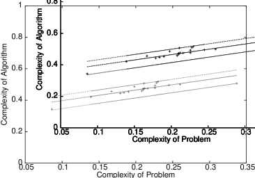
Figure 2: The regression line of the relationship between the complexity of the algorithm ${\cal A}$ and the complexity of the problem with the bounds including all points.

The experiment is repeated a number of times and each time the results confirm the consistency of the regression line (1). Therefore, within the accuracy of the linear regression, we are able to formulate an optimality condition: if the algorithm ${\cal A}$ shows its best performance for a problem $p$, then the complexity $C({\cal A}(p))$ of the algorithm ${\cal A}$ is in the linear relationship with the complexity $C(p)$ of the problem $p$

$$C({\cal A}(p))=0.67\times C(p)+0.33.$$ (2)

Computational investigations on the role of the PTM generator for the algorithm ${\cal A}$ suggest how the optimality condition (2) may be extended. For this reason we use a different algorithm ${\cal B}$, which works exactly in the same manner as the algorithm ${\cal A}$, except it consults a random generator instead of the PTM generator. To find a possible connection between the best performances and the relationship between the complexities, we compare the algorithms ${\cal A}$ and ${\cal B}$.

First, for each problem $p\in{\cal P}$ the best performance of the algorithm ${\cal A}$ is compared with the best performance of the algorithm ${\cal B}$. Fig. 3 shows that the algorithm ${\cal A}$ demonstrates significantly better results than the algorithm ${\cal B}$ for seventeen problems and results for the other three are close.

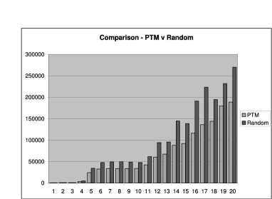
Figure 3: The best performances of the algorithm ${\cal A}$ using PTM generator are compared with the best performances of the algorithm ${\cal B}$ using random generator. The problems are ordered as in the description of the class $P$.

Second, we examine the relationship between the complexities of the algorithm ${\cal B}$ and the problem (Fig. 4) in the same manner as we have done for the algorithm ${\cal A}$ (Fig. 2). The situation deteriorates and the relationship is less consistent for the algorithm ${\cal B}$ in comparison with the algorithm ${\cal A}$. Formally, the calculated regression line

$$y=\alpha^{\prime}x+\beta^{\prime}=0.48x+0.23,$$

$$\alpha^{\prime}=0.48\pm 0.02,\ \ \ \beta^{\prime}=0.23\pm 0.01$$ (3)

is a less accurate estimator of the relationship between the complexities of the algorithm ${\cal B}$ and the problem. The standard error of estimate of $0.18$ and the absolute value of the maximal individual error of $0.1$ of the regression line (3) are doubled in comparison with the regression line (1). The coefficient of determination is only $0.26$ in comparison with $0.71$ for the algorithm ${\cal A}$.

Therefore, computationally, we reveal a connection between the best performances and the relationship between the complexities. In particular, the better result of the algorithm ${\cal A}$ (Fig. 3) corresponds to the fact that the relationship between the complexities of the algorithm ${\cal A}$ and the problem appears more consistent than it is in the case of the algorithm ${\cal B}$. In order to suggest potential implications of the optimality condition (2) to a wider context, we would like to use this proposition.

The observed connection allows us to assume a possible sequence of algorithms whose best performances converge to the optimal solutions of the problems as the relationships between the complexities converge to a certain function $g$. Notice, that the algorithms ${\cal A}$ and ${\cal B}$ may be well among the elements of the sequence with the algorithm ${\cal B}$ followed by the algorithm ${\cal A}$. According to the experiments, it seems likely that the function $g$ may be a linear function.

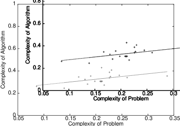
Figure 4: The regression line of the relationship between the complexity of the algorithm ${\cal B}$ and the complexity of the problem.

The possible convergence of the sequence would promise an algorithm ${\cal G}$ to link the optimal performance and the relationship between the complexities. As a result, the best performance of the algorithm ${\cal G}$ for any problem could actually provide the optimal solution. An optimality condition of the algorithm ${\cal G}$ may extend the optimality condition of the algorithm ${\cal A}$ and explain the optimal performance in terms of the relationship between the complexities: if the algorithm ${\cal G}$ shows its best performance for a problem $p$, and thus finds the optimum solution, then the complexity $C({\cal G}(p))$ of the algorithm is in the relationship $C({\cal G}(p))=g(C(p))$ with the complexity $C(p)$ of the problem.

The optimality condition of the algorithm ${\cal G}$ may suggest a new approach to optimization that would be primarily concerned with the efficient control of the algorithm’s complexity in matching the complexity of the problem. For example, if the algorithm ${\cal G}$ could potentially find the optimal solution to a problem $p$ of complexity $C(p)$ under the condition $C({\cal G}(p))=g(C(p))$, would it then be possible to obtain the optimal solution by a different algorithm working with the same complexity for the problem?

The ability to evaluate the complexity of the problem before the actual computation would be beneficial. In this case, the finding of the optimal solution could be connected with the tuning of the algorithm’s complexity in order to match the already known complexity of the problem. Experimentally, it is observed that for any problem the performance of the algorithm ${\cal A}$ is a convex function of the parameter. As a result, the best performance of the algorithm ${\cal A}$ for the problem can be efficiently obtained by the minimization of this convex function. Therefore, it would be important to understand whether the performance of the algorithm ${\cal G}$, as the function of its complexity, may behave in a similar way to provide us with efficient means for finding optimal solutions.

In conclusion, we have presented an optimization algorithm as a complex system. For any problem tested, the performance of the algorithm has been controlled as a convex function with a single optimum. By the characterization of the performance optimums, an optimality condition of the algorithm has been proposed. The optimality condition has revealed that the relationship between certain quantities of the complex system and the problem may determine the optimal performance. The result provides a computational evidence to the possibility of an optimality condition of complex systems.

This work was supported by CQU Research Advancement Awards Scheme grant no. IN9022 and Faculty of Informatics and Communication Research Grant Scheme no. FRG00406.

References

- (1) J. H. Holland Emergence: From Chaos to Order (Addison-Wesley, Reading, Massachusetts, 1998); Y. Bar-Yam Dynamics of Complex Systems (Westview Press, 1997); S. Kauffman At Home in the Universe (Oxford University Press, New York, 1995).
- (2) P. Ball, Nature 402, c73 (1999), and references therein.
- (3) G. Reinelt TSPLIB Version 1.2 online (ftp://ftp.wiwi.unifrankfurt.de/pub/TSPLIB 1.2) Accessed 28/11/2000.
- (4) V. Korotkikh A Mathematical Structure for Emergent Computation (Kluwer, Dordrecht, 1999).
- (5) M. Feigenbaum, Los Alamos Sci. 1, 4 (1980).
- (6) J. Allouche and M. Cosnard, in Dynamical Systems and Cellular Automata (Academic Press, 1985).
- (7) G. Korotkikh and V. Korotkikh, in Optimization and Industry: New Frontiers, edited by P. Pardalos and V. Korotkikh (Kluwer, Dordrecht, 2003).
- (8) V. Korotkikh and G. Korotkikh, in Quantitative Neuroscience, edited by P. Pardalos, C. Sackellares, P. Carney and L. Iasemidis (Kluwer, Dordrecht, 2004).
- (9) L. Sirovich and A.E. Deane, J. Fluid Mech. 222, 251 (1991); S. Ciliberto and B. Nikolaenko, Europhys. Lett. 14, 303 (1991); R. Vautard and M. Ghil, Physica (Amsterdam) 35D, 395 (1989).
- (10) S.M. Zoldi and H.S. Greenside, Phys. Rev. Lett. 78, 1687 (1997).