Componentwise Least Squares Support Vector Machines

Abstract

This chapter describes componentwise Least Squares Support Vector Machines (LS-SVMs) for the estimation of additive models consisting of a sum of nonlinear components. The primal-dual derivations characterizing LS-SVMs for the estimation of the additive model result in a single set of linear equations with size growing in the number of data-points. The derivation is elaborated for the classification as well as the regression case. Furthermore, different techniques are proposed to discover structure in the data by looking for sparse components in the model based on dedicated regularization schemes on the one hand and fusion of the componentwise LS-SVMs training with a validation criterion on the other hand.

keywords: LS-SVMs, additive models, regularization, structure detection

1 Introduction

Non-linear classification and function approximation is an important topic of interest with continuously growing research areas. Estimation techniques based on regularization and kernel methods play an important role. We mention in this context smoothing splines Wahba (1990), regularization networks Poggio and Girosi (1990), Gaussian processes MacKay (1992), Support Vector Machines (SVMs) Vapnik (1998); Cristianini and Shawe-Taylor (2000); Schoelkopf and Smola (2002) and many more, see e.g. Hastie et al. (2001). SVMs and related methods have been introduced within the context of statistical learning theory and structural risk minimization. In the methods one solves convex optimization problems, typically quadratic programs. Least Squares Support Vector Machines (LS-SVMs) Suykens and Vandewalle (1999); Suykens et al. (2002) are reformulations to standard SVMs which lead to solving linear KKT systems for classification tasks as well as regression. In Suykens et al. (2002) LS-SVMs have been proposed as a class of kernel machines with primal-dual formulations in relation to kernel Fisher Discriminant Analysis (FDA), Ridge Regression (RR), Partial Least Squares (PLS), Principal Component Analysis (PCA), Canonical Correlation Analysis (CCA), recurrent networks and control. The dual problems for the static regression without bias term are closely related to Gaussian processes MacKay (1992), regularization networks Poggio and Girosi (1990) and Kriging Cressie (1993), while LS-SVMs rather take an optimization approach with primal-dual formulations which have been exploited towards large scale problems and in developing robust versions.

Direct estimation of high dimensional nonlinear functions using a non-parametric technique without imposing restrictions faces the problem of the curse of dimensionality. Several attempts were made to overcome this obstacle, including projection pursuit regression Friedmann and Stuetzle (1981) and kernel methods for dimensionality reduction (KDR) Fukumizu et al. (2004). Additive models are very useful for approximating high dimensional nonlinear functions Stone (1985); Hastie and Tibshirani (1990). These methods and their extensions have become one of the widely used nonparametric techniques as they offer a compromise between the somewhat conflicting requirements of flexibility, dimensionality and interpretability. Traditionally, splines are a common modeling technique Wahba (1990) for additive models as e.g. in MARS (see e.g. Hastie et al. (2001)) or in combination with ANOVA Neter et al. (1974). Additive models were brought further to the attention of the machine learning community by e.g. Vapnik (1998); Gunn and Kandola (2002). Estimation of the nonlinear components of an additive model is usually performed by the iterative backfitting algorithm Hastie and Tibshirani (1990) or a two-stage marginal integration based estimator Linton and Nielsen (1995). Although consistency of both is shown under certain conditions, important practical problems (number of iteration steps in the former) and more theoretical problems (the pilot estimator needed for the latter procedure is a too generally posed problem) are still left.

In this chapter we show how the primal-dual derivations characterizing LS-SVMs can be employed to formulate a straightforward solution to the estimation problem of additive models using convex optimization techniques for classification as well as regression problems. Apart from this one-shot optimal training algorithm, the chapter approaches the problem of structure detection in additive models Hastie et al. (2001); Gunn and Kandola (2002) by considering an appropriate regularization scheme leading to sparse components. The additive regularization (AReg) framework Pelckmans et al. (2003) is adopted to emulate effectively these schemes based on 2-norms, 1-norms and specialized penalization terms Antoniadis and Fan (2001). Furthermore, a validation criterion is considered to select relevant components. Classically, exhaustive search methods (or stepwise procedures) are used which can be written as a combinatorial optimization problem. This chapter proposes a convex relaxation to the component selection problem.

This chapter is organized as follows. Section 2 presents componentwise LS-SVM regressors and classifiers for efficient estimation of additive models and relates the result with ANOVA kernels and classical estimation procedures. Section 3 introduces the additive regularization in this context and shows how to emulate dedicated regularization schemes in order to obtain sparse components. Section 4 considers the problem of component selection based on a validation criterion. Section 5 presents a number of examples.

2 Componentwise LS-SVMs and Primal-Dual Formulations

2.1 The Additive Model Class

Giving a training set defined as $\mathcal{D}_{N}=\{x_{k},y_{k}\}_{k=1}^{N}\subset\mathbb{R}^{D}\times\mathbb{R}$ of size $N$ drawn i.i.d. from an unknown distribution $F_{XY}$ according to $y_{k}=f(x_{k})+e_{k}$ where $f:\mathbb{R}^{D}\rightarrow\mathbb{R}$ is an unknown real-valued smooth function, $E[y_{k}|X=x_{k}]=f(x_{k})$ and $e_{1},\dots,e_{N}$ are uncorrelated random errors with $E\left[e_{k}|X=x_{k}\right]=0$, $E\left[(e_{k})^{2}|X=x_{k}\right]=\sigma_{e}^{2}<\infty$. The $n$ data points of the validation set are denoted as $\mathcal{D}_{n}^{(v)}=\{x^{(v)}_{j},y^{(v)}_{j}\}_{j=1}^{n}$. The following vector notations are used throughout the text: $X=\left(x_{1},\dots,x_{N}\right)\in\mathbb{R}^{D\times N}$, $Y=\left(y_{1},\dots,y_{N}\right)^{T}\in\mathbb{R}^{N}$, $X^{(v)}=\left(x^{(v)}_{1},\dots,x^{(v)}_{n}\right)\in\mathbb{R}^{D\times n}$ and $Y^{(v)}=\left(y^{(v)}_{1},\dots,y^{(v)}_{n}\right)^{T}\in\mathbb{R}^{n}$. The estimator of a regression function is difficult if the dimension $D$ is large. One way to quantify this is the optimal minimax rate of convergence $N^{-2l/(2l+D)}$ for the estimation of an $l$ times differentiable regression function which converges to zero slowly if $D$ is large compared to $l$ Stone (1982). A possibility to overcome the curse of dimensionality is to impose additional structure on the regression function. Although not needed in the derivation of the optimal solution, the input variables are assumed to be uncorrelated (see also concurvity Hastie and Tibshirani (1990)) in the applications.

Let superscript $x^{d}\in\mathbb{R}$ denote the $d$-th component of an input vector $x\in\mathbb{R}^{D}$ for all $d=1,\dots,D$. Let for instance each component correspond with a different dimension of the input observations. Assume that the function $f$ can be approximated arbitrarily well by a model having the following structure

$$f(x)=\sum_{d=1}^{D}f^{d}(x^{d})+b,$$ (1)

where $f^{d}:\mathbb{R}\rightarrow\mathbb{R}$ for all $d=1,\dots,D$ are unknown real-valued smooth functions and $b$ is an intercept term. The following vector notation is used: $X^{d}=\left(x^{d}_{1},\dots,x^{d}_{N}\right)\in\mathbb{R}^{1\times N}$ and $X^{(v)d}=\left(x^{(v)d}_{1},\dots,x^{(v)d}_{n}\right)\in\mathbb{R}^{1\times n}$. The optimal rate of convergence for estimators based on this model is $N^{-2l/(2l+1)}$ which is independent of $D$ Stone (1985). Most state-of-the-art estimation techniques for additive models can be divided into two approaches Hastie et al. (2001):

• Iterative approaches use an iteration where in each step part of the unknown components are fixed while optimizing the remaining components. This is motivated as:

  $$\hat{f}^{d_{1}}(x^{d_{1}}_{k})=y_{k}-e_{k}-\sum_{d_{2}\neq d_{1}}\hat{f}^{d_{2}}(x^{d_{2}}_{k}),$$ (2)

  for all $k=1,\dots,N$ and $d_{1}=1,\dots,D$. Once the $N-1$ components of the second term are known, it becomes easy to estimate the lefthandside. For a large class of linear smoothers, such so-called backfitting algorithms are equivalent to a Gauss-Seidel algorithm for solving a big ($ND\times ND$) set of linear equations Hastie et al. (2001). The backfitting algorithm Hastie and Tibshirani (1990) is theoretically and practically well motivated.

• Two-stages marginalization approaches construct in the first stage a general black-box pilot estimator (as e.g. a Nadaraya-Watson kernel estimator) and finally estimate the additive components by marginalizing (integrating out) for each component the variation of the remaining components.

2.2 Componentwise Least Squares Support Vector Machine Regressors

At first, a primal-dual formulation is derived for componentwise LS-SVM regressors. The global model takes the form as in (1) for any $x_{\ast}\in\mathbb{R}^{D}$

$$f(x_{\ast};w_{d},b)=\sum_{d=1}^{D}f^{d}(x_{\ast}^{d};w_{d})+b=\sum_{d=1}^{D}{w_{d}}^{T}\varphi_{d}(x_{\ast}^{d})+b.$$ (3)

The individual components of an additive model based on LS-SVMs are written as $f^{d}(x^{d};w_{d})=w_{d}^{T}\varphi_{d}(x^{d})$ in the primal space where $\varphi_{d}:\mathbb{R}\rightarrow\mathbb{R}^{n_{\varphi_{d}}}$ denotes a potentially infinite ($n_{\varphi_{d}}=\infty$) dimensional feature map. The regularized least squares cost function is given as Suykens et al. (2002)

$$\min_{{w_{d}},b,e_{k}}\mathcal{J}_{\gamma}(w_{d},e)=\frac{1}{2}\sum_{d=1}^{D}{w_{d}}^{T}w_{d}+\frac{\gamma}{2}\sum_{k=1}^{N}e_{k}^{2}\\ \text{ \ s.t. \ }\sum_{d=1}^{D}{w_{d}}^{T}\varphi_{d}(x^{d}_{k})+b+e_{k}=y_{k},\text{ \ \ }k=1,\dots,N.$$ (4)

Note that the regularization constant $\gamma$ appears here as in classical Tikhonov regularization Tikhonov and Arsenin (1977). The Lagrangian of the constraint optimization problem becomes

$$\mathcal{L}_{\gamma}(w_{d},b,e_{k};\alpha_{k})=\frac{1}{2}\sum_{d=1}^{D}{w_{d}}^{T}w_{d}+\frac{\gamma}{2}\sum_{k=1}^{N}e_{k}^{2}-\sum_{k=1}^{N}\alpha_{k}(\sum_{d=1}^{D}{w_{d}}^{T}\varphi_{d}(x_{k}^{d})+b+e_{k}-y_{k}).$$ (5)

By taking the conditions for optimality $\partial\mathcal{L}_{\gamma}/\partial\alpha_{k}=0$, $\partial\mathcal{L}_{\gamma}/\partial b=0$, $\partial\mathcal{L}_{\gamma}/\partial e_{k}=0$ and $\partial\mathcal{L}_{\gamma}/\partial w_{d}=0$ and application of the kernel trick $K^{d}(x^{d}_{k},x^{d}_{j})=\varphi_{d}(x^{d}_{k})^{T}\varphi_{d}(x^{d}_{j})$ with a positive definite (Mercer) kernel $K^{d}:\mathbb{R}\times\mathbb{R}\rightarrow\mathbb{R}$, one gets the following conditions for optimality

$$\left\{\begin{array}[]{rlrl}y_{k}&=\sum_{d=1}^{D}{w_{d}}^{T}\varphi_{d}(x_{k}^{d})+b+e_{k},&k=1,\dots,N&(a)\\ e_{k}\gamma&=\alpha_{k}&k=1,\dots,N&(b)\\ w_{d}&=\sum_{k=1}^{N}\alpha_{k}\varphi_{d}(x_{k}^{d})&d=1,\dots,D&(c)\\ 0&=\sum_{k=1}^{N}\alpha_{k}.&&(d)\end{array}\right.$$ (6)

Note that condition (6.b) states that the elements of the solution vector $\alpha$ should be proportional to the errors. The dual problem is summarized in matrix notation as

$$\left[\begin{tabular}[]{c|c}$0$&$1_{N}^{T}$\\ \hline\cr$1_{N}$&$\Omega+I_{N}/\gamma$\\ \end{tabular}\right]\left[\begin{tabular}[]{c}$b$\\ \hline\cr$\alpha$\\ \end{tabular}\right]=\left[\begin{tabular}[]{c}$0$\\ \hline\cr$Y$\\ \end{tabular}\right],$$ (7)

where $\Omega\in\mathbb{R}^{N\times N}$ with $\Omega=\sum_{d=1}^{D}\Omega^{d}$ and $\Omega^{d}_{kl}=K^{d}(x_{k}^{d},x_{l}^{d})$ for all $k,l=1,\dots,N$, which is expressed in the dual variables $\hat{\alpha}$ instead of $\hat{w}$. A new point $x_{\ast}\in\mathbb{R}^{D}$ can be evaluated as

$$\hat{y}_{\ast}=\hat{f}^{d}(x_{\ast};\hat{\alpha},\hat{b})=\sum_{k=1}^{N}\hat{\alpha}_{k}\sum_{d=1}^{D}K^{d}(x_{k}^{d},x_{\ast}^{d})+\hat{b},$$ (8)

where $\hat{\alpha}$ and $\hat{b}$ is the solution to (7). Simulating a validation datapoint $x_{j}$ for all $j=1,\dots,n$ by the $d$-th individual component

$$\hat{y}^{d}_{j}=\hat{f}^{d}(x_{j}^{d};\hat{\alpha})=\sum_{k=1}^{N}\hat{\alpha}_{k}K^{d}(x_{k}^{d},x_{j}^{d}),$$ (9)

which can be summarized as follows: $\hat{Y}=\left(\hat{y}_{1},\dots,\hat{y}_{N}\right)^{T}\in\mathbb{R}^{N}$, $\hat{Y}^{d}$ $=\left(\hat{y}^{d}_{1},\dots,\hat{y}^{d}_{N}\right)^{T}$ $\in\mathbb{R}^{N}$, $\hat{Y}^{(v)}=\left(\hat{y}^{(v)}_{1},\dots,\hat{y}^{(v)}_{n}\right)^{T}\in\mathbb{R}^{n}$ and $\hat{Y}^{(v)}_{d}=\left(\hat{y}^{(v)d}_{1},\dots,\hat{y}^{(v)d}_{n}\right)^{T}\in\mathbb{R}^{n}$.

Remarks:

• Note that the componentwise LS-SVM regressor can be written as a linear smoothing matrix Suykens et al. (2002):

  $$\hat{Y}=S_{\gamma}Y.$$ (10)

  For notational convenience, the bias term is omitted from this description. The smoother matrix $S_{\gamma}\in\mathbb{R}^{N\times N}$ becomes

  $$S_{\gamma}=\Omega\left(\Omega+I_{N}\frac{1}{\gamma}\right)^{-1}.$$ (11)

• The set of linear equations (7) corresponds with a classical LS-SVM regressor where a modified kernel is used

  $$K(x_{k},x_{j})=\sum_{d=1}^{D}K^{d}(x^{d}_{k},x_{j}^{d}).$$ (12)

  Figure 1 shows the modified kernel in case a one dimensional Radial Basis Function (RBF) kernel is used for all $D$ (in the example, $D=2$) components. This observation implies that componentwise LS-SVMs inherit results obtained for classical LS-SVMs and kernel methods in general. From a practical point of view, the previous kernels (and a fortiori componentwise kernel models) result in the same algorithms as considered in the ANOVA kernel decompositions as in Vapnik (1998); Gunn and Kandola (2002).

  $$K(x_{k},x_{j})=\sum_{d=1}^{D}K^{d}(x^{d}_{k},x_{j}^{d})+\sum_{d_{1}\neq d_{2}}K^{d_{1}d_{2}}\left((x_{k}^{d_{1}},x^{d_{2}}_{k})^{T},(x_{j}^{d_{1}},x_{j}^{d_{2}})^{T}\right)+\dots,$$ (13)

  where the componentwise LS-SVMs only consider the first term in this expansion. The described derivation as such bridges the gap between the estimation of additive models and the use of ANOVA kernels.

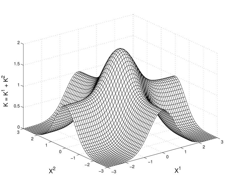
Figure 1: The two dimensional componentwise Radial Basis Function (RBF) kernel for componentwise LS-SVMs takes the form $K(x_{k},x_{l})=K^{1}(x^{1}_{k},x^{1}_{l})+K^{2}(x^{2}_{k},x^{2}_{l})$ as displayed. The standard RBF kernel takes the form $K(x_{k},x_{l})=\exp(-\|x_{k}-x_{l}\|^{2}_{2}/\sigma^{2})$ with $\sigma\in\mathbb{R}^{+}_{0}$ an appropriately chosen bandwidth.

2.3 Componentwise Least Squares Support Vector Machine Classifiers

In the case of classification, let $y_{k},y_{j}^{(v)}\in\{-1,1\}$ for all $k=1,\dots,N$ and $j=1,\dots,n$. The analogous derivation of the componentwise LS-SVM classifier is briefly reviewed. The following model is considered for modeling the data

$$f(x)={\rm sign}\left(\sum_{d=1}^{D}f^{d}(x^{d})+b\right),$$ (14)

where again the individual components of the additive model based on LS-SVMs are given as $f^{d}(x^{d})={w_{d}}^{T}\varphi_{d}(x^{d})$ in the primal space where $\varphi_{d}:\mathbb{R}\rightarrow\mathbb{R}^{n_{\varphi_{d}}}$ denotes a potentially infinite ($n_{\varphi_{d}}=\infty$) dimensional feature map. The regularized least squares cost function is given as Suykens and Vandewalle (1999); Suykens et al. (2002)

$$\min_{w_{d},b,e_{k}}\mathcal{J}_{\gamma}(w_{d},e)=\frac{1}{2}\sum_{d=1}^{D}{w_{d}}^{T}w_{d}+\frac{\gamma}{2}\sum_{k=1}^{N}e_{k}^{2}\\ \text{ \ s.t. \ }y_{k}\left(\sum_{d=1}^{D}{w_{d}}^{T}\varphi_{d}(x^{d}_{k})+b\right)=1-e_{k},\text{ \ \ }k=1,\dots,N,$$ (15)

where $e_{k}$ are so-called slack-variables for all $k=1,\dots,N$. After construction of the Lagrangian and taking the conditions for optimality, one obtains the following set of linear equations (see e.g. Suykens et al. (2002)):

$$\left[\begin{tabular}[]{c|c}$0$&$Y^{T}$\\ \hline\cr$Y$&$\Omega_{y}+I_{N}/\gamma$\\ \end{tabular}\right]\left[\begin{tabular}[]{c}$b$\\ \hline\cr$\alpha$\\ \end{tabular}\right]=\left[\begin{tabular}[]{c}$0$\\ \hline\cr$1_{N}$\\ \end{tabular}\right],$$ (16)

where $\Omega_{y}\in\mathbb{R}^{N\times N}$ with $\Omega_{y}=\sum_{d=1}^{D}\Omega^{d}_{y}\in\mathbb{R}^{N\times N}$ and $\Omega^{d}_{y,kl}=y_{k}y_{l}K^{d}(x_{k}^{d},x_{l}^{d})$. New data points $x_{\ast}\in\mathbb{R}^{D}$ can be evaluated as

$$\hat{y}_{\ast}={\rm sign}\left(\sum_{k=1}^{N}\hat{\alpha}_{k}y_{k}\sum_{d=1}^{D}K^{d}(x_{k}^{d},x_{\ast}^{d})+\hat{b}\right).$$ (17)

In the remainder of this text, only the regression case is considered. The classification case can be derived straightforwardly along the lines.

3 Regularizing for Sparse Components via Additive Regularization

A regularization method fixes a priori the answer to the ill-conditioned (or ill-defined) nature of the inverse problem. The classical Tikhonov regularization scheme Tikhonov and Arsenin (1977) states the answer in terms of the norm of the solution. The formulation of the additive regularization (AReg) framework Pelckmans et al. (2003) made it possible to impose alternative answers to the ill-conditioning of the problem at hand. We refer to this AReg level as substrate LS-SVMs. An appropriate regularization scheme for additive models is to favor solutions using the smallest number of components to explain the data as much as possible. In this paper, we use the somewhat relaxed condition of sparse components to select appropriate components instead of the more general problem of input (or component) selection.

3.1 Level 1: Componentwise LS-SVM Substrate

Figure 2: Graphical representation of the additive regularization framework used for emulating other loss functions and regularization schemes. Conceptually, one differentiates between the newly specified cost function and the LS-SVM substrate, while computationally both are computed simultanously.

Using the Additive Regularization (AReg) scheme for componentwise LS-SVM regressors results into the following modified cost function:

$$\min_{w_{d},b,e_{k}}\mathcal{J}_{c}(w_{d},e)=\frac{1}{2}\sum_{d=1}^{D}{w_{d}}^{T}w_{d}+\frac{1}{2}\sum_{k=1}^{N}(e_{k}-c_{k})^{2}\\ \text{ \ s.t. \ }\sum_{d=1}^{D}{w_{d}}^{T}\varphi_{d}(x^{d}_{k})+b+e_{k}=y_{k},\text{ \ \ }k=1,\dots,N,$$ (18)

where $c_{k}\in\mathbb{R}$ for all $k=1,\dots,N$. Let $c=(c_{1},\dots,c_{N})^{T}\in\mathbb{R}^{N}$. After constructing the Lagrangian and taking the conditions for optimality, one obtains the following set of linear equations, see Pelckmans et al. (2003):

$$\left[\begin{tabular}[]{c|c}$0$&$1_{N}^{T}$\\ \hline\cr$1_{N}$&$\Omega+I_{N}$\\ \end{tabular}\right]\left[\begin{tabular}[]{c}$b$\\ \hline\cr$\alpha$\\ \end{tabular}\right]+\left[\begin{tabular}[]{c}$0$\\ \hline\cr$c$\\ \end{tabular}\right]=\left[\begin{tabular}[]{c}$0$\\ \hline\cr$Y$\\ \end{tabular}\right]$$ (19)

and $e=\alpha+c\in\mathbb{R}^{N}$. Given a regularization constant vector $c$, the unique solution follows immediately from this set of linear equations.

However, as this scheme is too general for practical implementation, $c$ should be limited in an appropriate way by imposing for example constraints corresponding with certain model assumptions or a specified cost function. Consider for a moment the conditions for optimality of the componentwise LS-SVM regressor using a regularization term as in ridge regression, one can see that equation (7) corresponds with (19) if $\gamma^{-1}\alpha=\alpha+c$ for given $\gamma$. Once an appropriate $c$ is found which satisfies the constraints, it can be plugged in into the LS-SVM substrate (19). It turns out that one can omit this conceptual second stage in the computations by elimination of the variable $c$ in the constrained optimization problem (see Figure 2).

Alternatively, a measure corresponding with a (penalized) cost function can be used which fulfills the role of model selection in a broad sense. A variety of such explicit or implicit limitations can be emulated based on different criteria (see Figure 3).

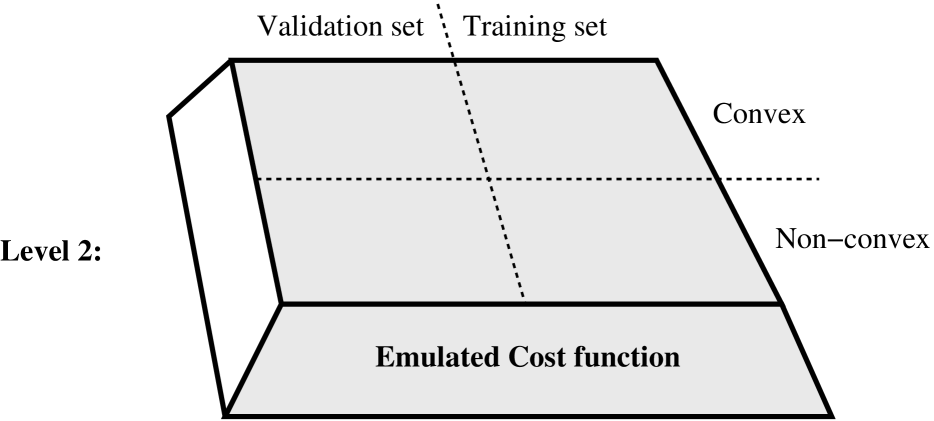
Figure 3: The level 2 cost functions of Figure 2 on the conceptual level can take different forms based on validation performance or trainings error. While some will result in convex tuning procedures, other may loose this property depending on the chosen cost function on the second level.

3.2 Level 2: Emulating an $L_{1}$ based Component Regularization Scheme (Convex)

We now study how to obtain sparse components by considering a dedicated regularization scheme. The LS-SVM substrate technique is used to emulate the proposed scheme as primal-dual derivations (see e.g. Subsection 2.2) are not straightforward anymore.

Let $\hat{Y}^{d}\in\mathbb{R}^{N}$ denote the estimated training outputs of the $d$-th submodel $f^{d}$ as in (9). The component based regularization scheme can be translated as the following constrained optimization problem where the conditions for optimality (18) as summarized in (19) are to be satisfied exactly (after elimination of $w$)

$$\min_{c,\hat{Y}^{d},e_{k};\alpha,b}\mathcal{J}_{\xi}(\hat{Y}^{d},e_{k})=\frac{1}{2}\sum_{d=1}^{D}\|\hat{Y}^{d}\|_{1}+\frac{\xi}{2}\sum_{k=1}^{N}e_{k}^{2}\\ \text{ \ s.t. \ }\left\{\begin{array}[]{l}1_{N}^{T}\alpha=0,\\ \Omega\,\alpha+1_{N}^{T}b+\alpha+c=Y,\\ \Omega^{d}\,\alpha=\hat{Y}^{d},\ \ \ \forall d=1,\dots,D\\ \alpha+c=e,\end{array}\right.$$ (20)

where the use of the robust $L_{1}$ norm can be justified as in general no assumptions are imposed on the distribution of the elements of $\hat{Y}^{d}$. By elimination of $c$ using the equality $e=\alpha+c$, this problem can be written as follows

1NΩ0NΩ1⋮⋮0NΩd]​[bα]+[ eY^1⋮Y^D]=[ Y0N⋮0N].subscriptsuperscript^𝑌𝑑subscript𝑒𝑘𝛼𝑏subscript𝒥𝜉superscript^𝑌𝑑subscript𝑒𝑘12superscriptsubscript𝑑1𝐷subscriptdelimited-∥∥superscript^𝑌𝑑1𝜉2superscriptsubscript𝑘1𝑁superscriptsubscript𝑒𝑘2 s.t. delimited-[]fragments fragments1𝑁Ωfragments0𝑁fragmentsΩ1⋮⋮fragments0𝑁fragmentsΩ𝑑delimited-[]𝑏𝛼delimited-[] 𝑒fragments^𝑌1⋮fragments^𝑌𝐷delimited-[] 𝑌fragments0𝑁⋮fragments0𝑁\min_{\hat{Y}^{d},e_{k};\alpha,b}\mathcal{J}_{\xi}(\hat{Y}^{d},e_{k})=\frac{1}{2}\sum_{d=1}^{D}\|\hat{Y}^{d}\|_{1}+\frac{\xi}{2}\sum_{k=1}^{N}e_{k}^{2}\\ \text{ \ s.t. \ }\left[\begin{tabular}[]{c|c}$0$&$1_{N}^{T}$\\ \hline\cr$1_{N}$&$\Omega$\\ \hline\cr$0_{N}$&$\Omega^{1}$\\ $\vdots$&$\vdots$\\ $0_{N}$&$\Omega^{d}$\\ \end{tabular}\right]\left[\begin{tabular}[]{c}$b$\\ \hline\cr$\alpha$\\ \end{tabular}\right]+\left[\begin{tabular}[]{c}$0$\\ \hline\cr$e$\\ \hline\cr$\hat{Y}^{1}$\\ $\vdots$\\ $\hat{Y}^{D}$\\ \end{tabular}\right]=\left[\begin{tabular}[]{c}$0$\\ \hline\cr$Y$\\ \hline\cr$0_{N}$\\ $\vdots$\\ $0_{N}$\\ \end{tabular}\right].

01NT0001NT00 (21)

This convex constrained optimization problem can be solved as a quadratic programming problem. As a consequence of the use of the $L_{1}$ norm, often sparse components ($\|\hat{Y}^{d}\|_{1}=0$) are obtained, in a similar way as sparse variables of LASSO or sparse datapoints in SVM Hastie et al. (2001); Vapnik (1998). An important difference is that the estimated outputs are used for regularization purposes instead of the solution vector. It is good practice to omit sparse components on the training dataset from simulation:

$$\hat{f}(x_{\ast};\hat{\alpha},\hat{b})=\sum_{i=1}^{N}\hat{\alpha}_{i}\sum_{d\in\mathcal{S}_{D}}K^{d}(x_{i}^{d},x_{\ast}^{d})+\hat{b},$$ (22)

where $\mathcal{S}_{D}=\{d|\hat{\alpha}^{T}\Omega^{d}\hat{\alpha}\neq 0\}$.

Using the $L_{2}$ norm $\sum_{d=1}^{D}\|\hat{Y}^{d}\|_{2}^{2}$ instead leads to a much simpler optimization problem, but additional assumptions (Gaussianity) are needed on the distribution of the elements of $\hat{Y}^{d}$. Moreover, the component selection has to resort on a significance test instead of the sparsity resulting from (21). A practical algorithm is proposed in Subsection 5.1 that uses an iteration of $L_{2}$ norm based optimizations in order to calculate the optimum of the proposed regularized cost function.

3.3 Level 2 bis: Emulating a Smoothly Thresholding Penalty Function (Non-convex)

This subsection considers extensions to classical formulations towards the use of dedicated regularization schemes for sparsifying components. Consider the componentwise regularized least squares cost function defined as

$$\mathcal{J}_{\lambda}(w_{d},e)=\frac{\lambda}{2}\sum_{d=1}^{D}\ell(w_{d})+\frac{1}{2}\sum_{k=1}^{N}e^{2}_{k},$$ (23)

where $\ell(w_{d})$ is a penalty function and $\lambda\in\mathbb{R}_{0}+$ acts as a regularization parameter. We denote $\lambda\ell(\cdot)$ by $\ell_{\lambda}(\cdot)$, so it may depend on $\lambda$. Examples of penalty functions include:

• The $L_{p}$ penalty function $\ell_{\lambda}^{p}(w_{d})=\lambda\|w_{d}\|^{p}_{p}$ leads to a bridge regression Frank and Friedman (1993); Fu (1998). It is known that the $L_{2}$ penalty function $p=2$ results in the ridge regression. For the $L_{1}$ penalty function the solution is the soft thresholding rule Donoho and Johnstone (1994). LASSO, as proposed by Tibshirani (1996, 1997), is the penalized least squares estimate using the $L_{1}$ penalty function (see Figure 4.a).

• Let the indicator function $I_{\{x\in\mathcal{A}\}}=1$ if $x\in\mathcal{A}$ for a specified set $\mathcal{A}$ and 0 otherwise. When the penalty function is given by $\ell_{\lambda}(w_{d})=\lambda^{2}-(\|w_{d}\|_{1}-\lambda)^{2}I_{\{\|w_{d}\|_{1}<\lambda\}}$ (see Figure 4.b), the solution is a hard-thresholding rule Antoniadis (1997).

The $L_{p}$ and the hard thresholding penalty functions do not simultaneously satisfy the mathematical conditions for unbiasedness, sparsity and continuity Fan and Li (2001). The hard thresholding has a discontinuous cost surface. The only continuous cost surface (defined as the cost function associated with the solution space) with a thresholding rule in the $L_{p}$-family is the $L_{1}$ penalty function, but the resulting estimator is shifted by a constant $\lambda$. To avoid these drawbacks, Nikolova (1999) suggests the penalty function defined as

$$\ell_{\lambda}^{a}(w_{d})=\frac{\lambda a\|w_{d}\|_{1}}{1+a\|w_{d}\|_{1}},$$ (24)

with $a\in\mathbb{R}_{0}^{+}$. This penalty function behaves quite similarly as the Smoothly Clipped Absolute Deviation (SCAD) penalty function as suggested by Fan (1997). The Smoothly Thresholding Penalty (TTP) function (24) improves the properties of the $L_{1}$ penalty function and the hard thresholding penalty function (see Figure 4.c), see Antoniadis and Fan (2001). The unknowns $a$ and $\lambda$ act as regularization parameters. A plausible value for $a$ was derived in Nikolova (1999); Antoniadis and Fan (2001) as $a=3.7$.

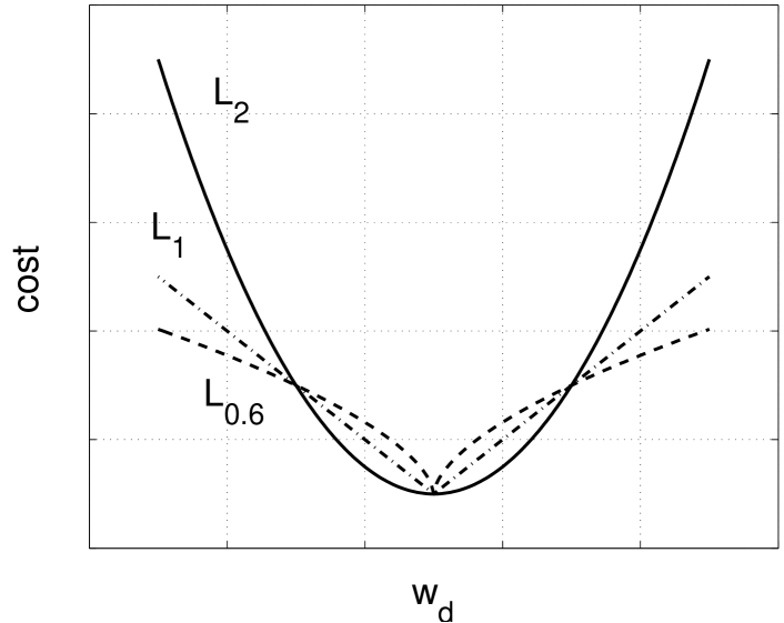
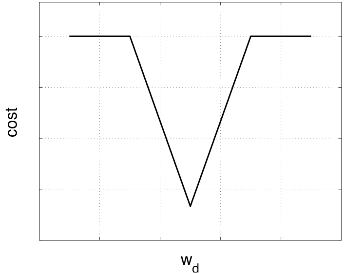
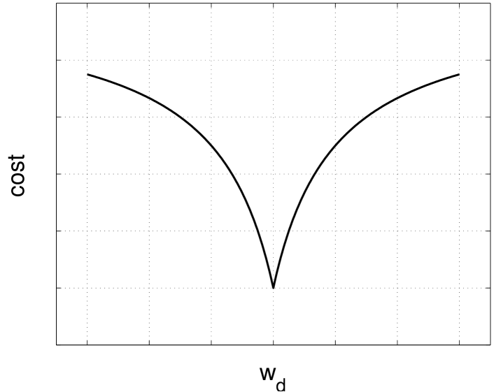
Figure 4: Typical penalty functions: (a) the $L_{p}$ penalty family for $p=2,1$ and $0.6$, (b) hard thresholding penalty function and (c) the transformed $L_{1}$ penalty function.

The transformed $L_{1}$ penalty function satisfies the oracle inequalities Donoho and Johnstone (1994). One can plugin the described semi-norm $\ell_{\lambda}^{a}(\cdot)$ to improve the component based regularization scheme (20). Again, the additive regularization scheme is used for the emulation of this scheme

$$\min_{c,\hat{Y}^{d},e_{k};\alpha,b}\mathcal{J}_{\lambda}(\hat{Y}^{d},e_{k})=\frac{1}{2}\sum_{d=1}^{D}\ell_{\lambda}^{a}(\hat{Y}^{d})+\frac{1}{2}\sum_{k=1}^{N}e_{k}^{2}\\ \text{ \ s.t. \ }\left\{\begin{array}[]{l}1_{N}^{T}\alpha=0,\\ \Omega\,\alpha+1_{N}^{T}b+\alpha+c=Y,\\ \Omega^{d}\,\alpha=\hat{Y}^{d},\ \ \ \forall d=1,\dots,D\\ \alpha+c=e,\end{array}\right.$$ (25)

which becomes non-convex but can be solved using an iterative scheme as explained later in Subsection 5.1.

4 Fusion of Componentwise LS-SVMs and Validation

This section investigates how one can tune the componentwise LS-SVMs with respect to a validation criterion in order to improve the generalization performance of the final model. As proposed in Pelckmans et al. (2003), fusion of training and validation levels can be investigated from an optimization point of view, while conceptually they are to be considered at different levels.

4.1 Fusion of Componentwise LS-SVMs and Validation for Regularization Constant Tuning

For this purpose, the fusion argument as introduced in Pelckmans et al. (2003) is briefly revised in relation to regularization parameter tuning. The estimator of the LS-SVM regressor on the training data for a fixed value $\gamma$ is given as (4)

$${\bf Level\ 1:\ \ }(\hat{w},\hat{b})=\operatorname*{\arg\min}_{w,b,e}\mathcal{J}_{\gamma}(w,e)\mbox{ \ \ s.t. (\ref{eq.clssvmr.cost}) holds,}$$ (26)

which results into solving a linear set of equations (7) after substitution of $w$ by Lagrange multipliers $\alpha$. Tuning the regularization parameter by using a validation criterion gives the following estimator

$${\bf Level\ 2:\ \ }\hat{\gamma}=\operatorname*{\arg\min}_{\gamma}\sum_{j=1}^{n}\left(f(x_{j};\hat{\alpha},\hat{b})-y_{j}\right)^{2}\mbox{ \ \ with \ \ }(\hat{\alpha},\hat{b})=\operatorname*{\arg\min}_{\alpha,b}\mathcal{J}_{\gamma}$$ (27)

satisfying again (4). Using the conditions for optimality (7) and eliminating $w$ and $e$

$${\bf Fusion:\ \ }(\hat{\gamma},\hat{\alpha},\hat{b})=\operatorname*{\arg\min}_{\gamma,\alpha,b}\sum_{j=1}^{n}\left(f(x_{j};\alpha,b)-y_{j}\right)^{2}\mbox{ \ \ s.t. \ \ (\ref{eq.clssvmr.train}) holds,}\hskip 28.45274pt$$ (28)

which is referred to as fusion. The resulting optimization problem was noted to be non-convex as the set of optimal solutions $w$ (or dual $\alpha$’s) corresponding with a $\gamma>0$ is non-convex. To overcome this problem, a re-parameterization of the trade-off was proposed leading to the additive regularization scheme. At the cost of overparameterizing the trade-off, convexity is obtained. To circumvent this drawback, different ways to restrict explicitly or implicitly the (effective) degrees of freedom of the regularization scheme $c\in\mathcal{A}\subset\mathbb{R}^{N}$ were proposed while retaining convexity (Pelckmans et al. (2003)). The convex problem resulting from additive regularization is

$${\bf Fusion:\ \ }(\hat{c},\hat{\alpha},\hat{b})=\operatorname*{\arg\min}_{c\in\mathcal{A},\alpha,b}\sum_{j=1}^{n}\left(f(x_{j};\alpha,b)-y_{j}\right)^{2}\mbox{ \ \ s.t. \ \ (\ref{eq.areg.train}) holds},\hskip 28.45274pt$$ (29)

and can be solved efficiently as a convex constrained optimization problem if $\mathcal{A}$ is a convex set, resulting immediately in the optimal regularization trade-off and model parameters Boyd and Vandenberghe (2004).

4.2 Fusion for Component Selection using the Additive Regularization Scheme

One possible relaxed version of the component selection problem goes as follows: Investigate whether it is plausible to drive the components on the validation set to zero without too large modifications on the global training solution. This is translated as the following cost function much in the spirit of (20). Let $\Omega^{(v)}$ denote $\sum_{d=1}^{D}\Omega^{(v)d}\in\mathbb{R}^{n\times N}$ and $\Omega^{(v)d}_{jk}=K^{d}(x^{(v)d}_{j},x_{k}^{d})$ for all $j=1,\dots,n$ and $k=1,\dots,N$.

$$(\hat{c},\hat{Y}^{(v)d},\hat{w}_{d},\hat{e},\hat{\alpha},\hat{b})=\operatorname*{\arg\min}_{c,\hat{Y}^{d},\hat{Y}^{(v)d},e,\alpha,b}\frac{1}{2}\sum_{d=1}^{D}\|\hat{Y}^{(v)d}\|_{1}+\frac{1}{2}\sum_{d=1}^{D}\|\hat{Y}^{d}\|_{1}+\frac{\xi}{2}\sum_{k=1}^{N}e_{k}^{2}\\ \text{ \ s.t. \ }\left\{\begin{array}[]{l}1_{N}^{T}\alpha=0\\ \alpha+c=e\\ \Omega\,\alpha+1_{N}b+\alpha+c=Y\\ \Omega^{d}\,\alpha=\hat{Y}^{d},\ \ \ \forall d=1,\dots,D,\\ \Omega^{(v)d}\,\alpha=\hat{Y}^{(v)d},\ \ \ \forall d=1,\dots,D,\end{array}\right.$$ (30)

where the equality constraints consist of the conditions for optimality of (19) and the evaluation of the validation set on the individual components. Again, this convex problem can be solved as a quadratic programming problem.

4.3 Fusion for Component Selection using Componentwise Regularized LS-SVMs

We proceed by considering the following primal cost function for a fixed but strictly positive $\eta=(\eta_{1},\dots,\eta_{D})^{T}\in(\mathbb{R}_{0}^{+})^{D}$

$${\bf Level\ 1:\ \ }\min_{{w_{d}},b,e_{k}}\mathcal{J}_{\eta}(w_{d},e)=\frac{1}{2}\sum_{d=1}^{D}\frac{{w_{d}}^{T}w_{d}}{\eta_{d}}+\frac{1}{2}\sum_{k=1}^{N}e_{k}^{2}\\ \text{ \ s.t. \ }\sum_{d=1}^{D}{w_{d}}^{T}\varphi_{d}(x^{d}_{k})+b+e_{k}=y_{k},\text{ \ \ }k=1,\dots,N.$$ (31)

Note that the regularization vector appears here similar as in the Tikhonov regularization scheme Tikhonov and Arsenin (1977) where each component is regularized individually. The Lagrangian of the constrained optimization problem with multipliers $\alpha^{\eta}\in\mathbb{R}^{N}$ becomes

$$\mathcal{L}_{\eta}(w_{d},b,e_{k};\alpha_{k})=\frac{1}{2}\sum_{d=1}^{D}\frac{{w_{d}}^{T}w_{d}}{\eta_{d}}+\frac{1}{2}\sum_{k=1}^{N}e_{k}^{2}\\ -\sum_{k=1}^{N}\alpha^{\eta}_{k}(\sum_{d=1}^{D}{w_{d}}^{T}\varphi_{d}(x_{k}^{d})+b+e_{k}-y_{k}).$$ (32)

By taking the conditions for optimality $\partial\mathcal{L}_{\eta}/\partial\alpha_{k}=0$, $\partial\mathcal{L}_{\eta}/\partial b=0$, $\partial\mathcal{L}_{\eta}/\partial e_{k}=0$ and $\partial\mathcal{L}_{\eta}/\partial w_{d}=0$, one gets the following conditions for optimality

$$\left\{\begin{array}[]{rlrl}y_{k}&=\sum_{d=1}^{D}{w_{d}}^{T}\varphi_{d}(x_{k}^{d})+b+e_{k},&k=1,\dots,N&(a)\\ e_{k}&=\alpha^{\eta}_{k},&k=1,\dots,N&(b)\\ w_{d}&=\eta_{d}\sum_{k=1}^{N}\alpha^{\eta}_{k}\varphi_{d}(x_{k}^{d}),&d=1,\dots,D&(c)\\ 0&=\sum_{k=1}^{N}\alpha^{\eta}_{k}.&&(d)\end{array}\right.$$ (33)

The dual problem is summarized in matrix notation by application of the kernel trick,

$$\left[\begin{tabular}[]{c|c}$0$&$1_{N}^{T}$\\ \hline\cr$1_{N}$&$\Omega^{\eta}+I_{N}$\\ \end{tabular}\right]\left[\begin{tabular}[]{c}$b$\\ \hline\cr$\alpha^{\eta}$\\ \end{tabular}\right]=\left[\begin{tabular}[]{c}$0$\\ \hline\cr$Y$\\ \end{tabular}\right],$$ (34)

where $\Omega^{\eta}\in\mathbb{R}^{N\times N}$ with $\Omega^{\eta}=\sum_{d=1}^{D}\eta_{d}\Omega^{d}$ and $\Omega^{d}_{kl}=K^{d}(x_{k}^{d},x_{l}^{d})$. A new point $x_{\ast}\in\mathbb{R}^{D}$ can be evaluated as

$$\hat{y}_{\ast}=\hat{f}(x_{\ast};\hat{\alpha}^{\eta},\hat{b})=\sum_{k=1}^{N}\hat{\alpha}^{\eta}_{k}\sum_{d=1}^{D}\eta_{d}K^{d}(x_{k}^{d},x_{\ast}^{d})+\hat{b},$$ (35)

where $\hat{\alpha}$ and $\hat{b}$ are the solution to (34). Simulating a training datapoint $x_{k}$ for all $k=1,\dots,N$ by the $d$-th individual component

$$\hat{y}^{\eta,d}_{k}=\hat{f}^{d}(x_{k}^{d};\hat{\alpha}^{\eta})=\eta_{d}\sum_{l=1}^{N}\hat{\alpha}^{\eta}_{l}K^{d}(x_{k}^{d},x_{l}^{d}),$$ (36)

which can be summarized in a vector $\hat{Y}^{\eta,d}=(\hat{y}^{d}_{1},\dots,\hat{y}^{d}_{N})\in\mathbb{R}^{N}$. As in the previous section, the validation performance is used for tuning the regularization parameters

$${\bf\small Level\ 2:\ \ }\hat{\eta}=\operatorname*{\arg\min}_{\eta}\sum_{j=1}^{n}\left(f(x_{j};\hat{\alpha}^{\eta},\hat{b})-y_{j}\right)^{2}\mbox{ \ \ with \ \ }(\hat{\alpha}^{\eta},\hat{b})=\operatorname*{\arg\min}_{\alpha^{\eta},b}\mathcal{J}_{\eta},$$ (37)

or using the conditions for optimality (34) and eliminating $w$ and $e$

$${\bf\small Fusion:\ \ }(\hat{\eta},\hat{\alpha}^{\eta},\hat{b})=\operatorname*{\arg\min}_{\eta,\alpha^{\eta},b}\sum_{j=1}^{n}\left(f(x_{j};\alpha^{\eta},b)-y_{j}\right)^{2}\mbox{ \ \ s.t. \ \ (\ref{eq.fusionc.train}) holds},\hskip 28.45274pt$$ (38)

which is a non-convex constrained optimization problem.

Embedding this problem in the additive regularization framework will lead us to a more suitable representation allowing for the use of dedicated algorithms. By relating the conditions (19) to (34), one can view the latter within the additive regularization framework by imposing extra constraints on $c$. The bias term $b$ is omitted from the remainder of this subsection for notational convenience. The first two constraints reflect training conditions for both schemes. As the solutions $\alpha^{\eta}$ and $\alpha$ do not have the same meaning (at least for model evaluation purposes, see (8) and (35)), the appropriate $c$ is determined here by enforcing the same estimation on the training data. In summary:

$$\left\{\begin{array}[]{l}\left(\Omega+I_{N}\right)\alpha+c=Y\\ \left(\left(\sum_{d=1}^{D}\eta_{d}\Omega^{d}\right)+I_{N}\right)\alpha^{\eta}=Y\\ \left(\sum_{d=1}^{D}\eta_{d}\Omega^{d}\right)\alpha^{\eta}=\Omega\alpha\end{array}\right.\Rightarrow\left\{\begin{array}[]{l}\left(\Omega+I_{N}\right)\alpha+c=Y\\ \Omega\alpha=\eta^{T}\otimes I_{N}\left[\begin{tabular}[]{c}$\Omega^{1}$\\ $\ldots$\\ $\Omega^{D}$\\ \end{tabular}\right](\alpha+c),\end{array}\right.$$ (39)

where the second set of equations is obtained by eliminating $\alpha^{\eta}$. The last equation of the righthand side represents the set of constraints of the values $c$ for all possible values of $\eta$. The product $\otimes$ denotes $\eta^{T}\otimes I_{N}=[\eta_{1}I_{N},\dots,\eta_{D}I_{N}]\in\mathbb{R}^{N\times ND}$. As for the Tikhonov case, it is readily seen that the solution space of $c$ with respect to $\eta$ is non-convex, however, the constraint on $c$ is recognized as a bilinear form. The fusion problem (38) can be written as

$${\bf\small Fusion:\ \ }(\hat{\eta},\hat{\alpha},\hat{c})=\operatorname*{\arg\min}_{\eta,\alpha,c}\left\|\Omega^{(v)}\alpha-Y^{(v)}\right\|^{2}_{2}\mbox{ \ \ s.t. \ \ (\ref{eq.fusionc.c}) holds},\hskip 28.45274pt$$ (40)

where algorithms as alternating least squares can be used.

5 Applications

For practical applications, the following iterative approach is used for solving non-convex cost-functions as (25). It can also be used for the efficient solution of convex optimization problems which become computational heavy in the case of a large number of datapoints as e.g. (21). A number of classification as well as regression problems are employed to illustrate the capabilities of the described approach. In the experiments, hyper-parameters as the kernel parameter (taken to be constants over the components) and the regularization trade-off parameter $\gamma$ or $\xi$ were tuned using $10$-fold cross-validation.

5.1 Weighted Graduated Non-Convexity Algorithm

An iterative scheme was developed based on the graduated non-convexity algorithm as proposed in Blake (1989); Nikolova (1999); Antoniadis and Fan (2001) for the optimization of non-convex cost functions. Instead of using a local gradient (or Newton) step which can be quite involved, an adaptive weighting scheme is proposed: in every step, the relaxed cost function is optimized by using a weighted 2-norm where the weighting terms are chosen based on an initial guess for the global solution. For every symmetric loss function $\ell(|e|):\mathbb{R}^{+}\rightarrow\mathbb{R}^{+}$ which is monotonically increasing, there exists a bijective transformation $t:\mathbb{R}\rightarrow\mathbb{R}$ such that for every $e=y-f(x;\theta)\in\mathbb{R}$

$$\ell(e)=\left(t(e)\right)^{2}.$$ (41)

The proposed algorithm for computing the solution for semi-norms employs iteratively convex relaxations of the prescribed non-convex norm. It is somewhat inspired by the simulated annealing optimization technique for optimizing global optimization problems. The weighted version is based on the following derivation

$$\ell(e_{k})=(\nu_{k}e_{k})^{2}\Leftrightarrow\nu_{k}=\sqrt{\frac{\ell(e_{k})}{e^{2}_{k}}},$$ (42)

where the $e_{k}$ for all $k=1,\dots,N$ are the residuals corresponding with the solutions to $\theta=\operatorname*{\arg\min}_{\theta}\ell\left(y_{k}-f(x_{k};\theta)\right)$

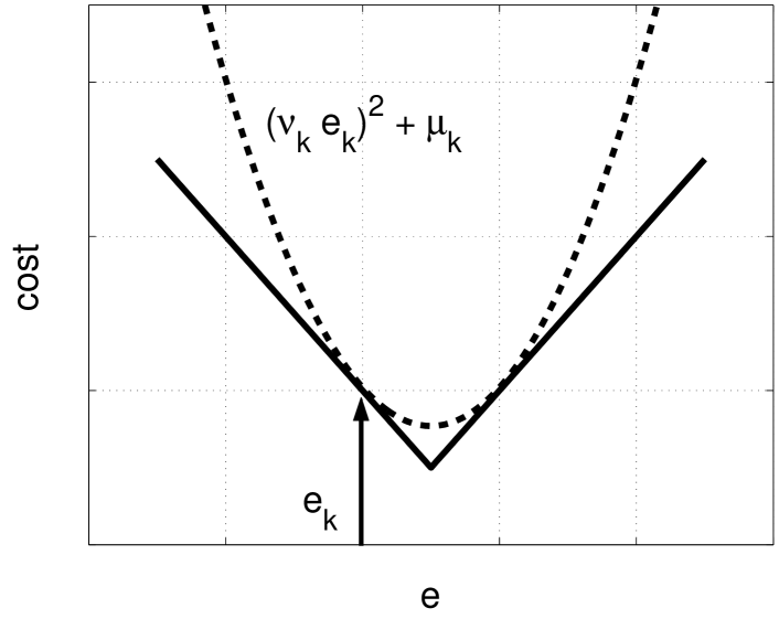
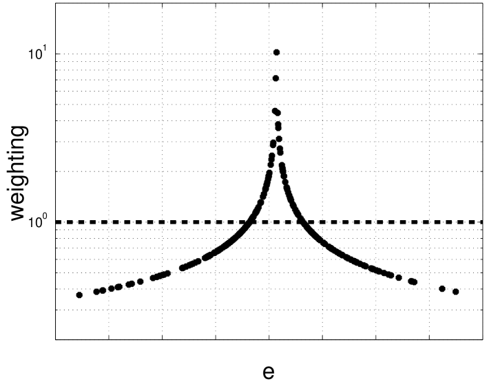
Figure 5: (a) Weighted $L_{2}$-norm (dashed) approximation $(\nu_{k}e_{k})^{2}+\mu_{k}$ of the $L_{1}$-norm (solid) $\ell(e)=|e|_{1}$ which follows from the linear set of equations (43) once the optimal $e_{k}$ are known; (b) the weighting terms $\nu_{k}$ for a sequence of $e_{k}$ and $k=1,\dots,N$ such that $(\nu_{k}e_{k})^{2}+\mu_{k}=|e_{k}|_{1}$ and $2\nu_{k}^{2}e_{k}=l^{\prime}(e_{k})={\rm sign}(e_{k})$ for an appropriate $\mu_{k}$.

This is equal to the solution of the convex optimization problem $e_{k}=\operatorname*{\arg\min}_{\theta}\left(\nu_{k}(y_{k}-f(x_{k};\theta))\right)^{2}$ for a set of $\nu_{k}$ satisfying (42). For more stable results, the gradient of the penalty function $\ell$ and the quadratic approximation can be takne equal as follows by using an intercept parameter $\mu_{k}\in\mathbb{R}$ for all $k=1,\dots,N$:

$$\left\{\begin{array}[]{rl}\ell(e_{k})&=(\nu_{k}e_{k})^{2}+\mu_{k}\\ \ell^{\prime}(e_{k})&=2\nu^{2}_{k}e_{k}\end{array}\right.\Leftrightarrow\left[\begin{tabular}[]{c|c}$e^{2}_{k}$&$1$\\ \hline\cr$2e_{k}$&$0$\\ \end{tabular}\right]\left[\begin{tabular}[]{c}$\nu_{k}^{2}$\\ \hline\cr$\mu_{k}$\\ \end{tabular}\right]=\left[\begin{tabular}[]{c}$\ell(e_{k})$\\ \hline\cr$\ell^{\prime}(e_{k})$\\ \end{tabular}\right],$$ (43)

where $\ell^{\prime}(e_{k})$ denotes the derivative of $\ell$ evaluated in $e_{k}$ such that a minimum of $\mathcal{J}_{\ell}$ also minimizes the weighted equivalent (the derivatives are equal). Note that the constant intercepts $\mu_{k}$ are not relevant in the weighted optimization problem. Under the assumption that the two consecutive relaxations $\ell^{(t)}$ and $\ell^{(t+1)}$ do not have too different global solutions, the following algorithm is a plausible practical tool:

Algorithm 1 (Weighted Graduated Non-Convexity Algorithm)

For the optimization of semi-norms ($\ell(\cdot)$), a practical approach is based on deforming gradually a 2-norm into the specific loss function of interest. Let $\zeta$ be a strictly decreasing series $1,\zeta^{(1)},\zeta^{(2)},\dots,0$. A plausible choice for the initial convex cost function is the least squares cost function $\mathcal{J}_{\rm LS}(e)=\|e\|_{2}^{2}$.

1. Compute the solution $\theta^{(0)}$ for $L_{2}$ norm $J_{\rm LS}(e)=\|e\|_{2}^{2}$ with residuals $e_{k}^{(0)}$;

2. $t=0$ and $\nu^{(0)}=1_{N}$;

3. Consider the following relaxed cost function $\mathcal{J}^{(t)}(e)=(1-\zeta_{t})\ell(e)+\zeta_{t}\mathcal{J}_{\rm LS}(e)$;

4. Estimate the solution $\theta^{(t+1)}$ and corresponding residuals $e_{k}^{(t+1)}$ of the cost function $\mathcal{J}^{(t)}$ using the weighted approximation $\mathcal{J}_{\rm approx}=(\nu_{k}^{(t)}e_{k})^{2}$ of $J^{(t)}(e_{k})$

5. Reweight the residuals using weighted approximative squares norms as derived in (43):

6. $t:=t+1$ and iterate step (3,4,5,6) until convergence.

When iterating this scheme, most $\nu_{k}$ will be smaller than $1$ as the least squares cost function penalizes higher residuals (typically outliers). However, a number of residuals will have increasing weight as the least squares loss function is much lower for small residuals.

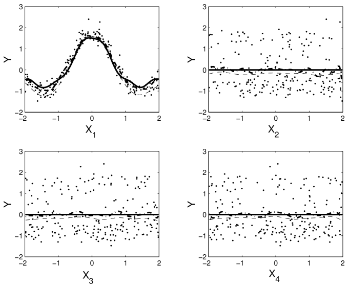
Figure 6: Example of a toy dataset consisting of four input components $X^{1},X^{2},X^{3}$ and $X^{4}$ where only the first one is relevant to predict the output $f(x)={\rm sinc}(x^{1})$. A componentwise LS-SVM regressor (dashed line) has good prediction performance, while the $L_{1}$ penalized cost function of Subsection (3.2) also recovers the structure in the data as the estimated components correspnding with $X^{2},X^{3}$ and $X^{4}$ are sparse.

5.2 Regression examples

To illustrate the additive model estimation method, a classical example was constructed as in Hastie and Tibshirani (1990); Vapnik (1998). The data were generated according to $y_{k}=10\,{\rm sinc}(x^{1}_{k})+20\,(x^{2}_{k}-0.5)^{2}+10\,x^{3}_{k}+5\,x^{4}_{k}+e_{k}$ were $e_{k}\sim\mathcal{N}(0,1)$, $N=100$ and the input data $X$ are randomly chosen from the interval $[0,1]^{10}$. Because of the Gaussian nature of the noise model, only results from least squares methods are reported. The described techniques were applied on this training dataset and tested on an independent test set generated using the saem rules. Table 1 reports whether the algorithm recovered the structure in the data (if so, the measure is 100%). The experiment using the smoothly tresholding penalized (STP) cost function was designed as follows: for every 10 components, a version was provided for the algorithm for the use of a linear kernel and another for the use of a RBF kernel (resulting in 20 new components). The regularization scheme was able to select the components with the appropriate kernel (a nonlinear RBF kernel for $X^{1}$ and $X^{2}$ and linear ones for $X^{3}$ and $X^{4}$), except for one spurious component (A RBF kernel was selected for the fifth component).

Method	Test set Performance			Sparse components
	$L_{2}$	$L_{1}$	$L_{\infty}$	% recovered
LS-SVMs	0.1110	0.2582	0.8743	0%
componentwise LS-SVMs (7)	0.0603	0.1923	0.6249	0%
$L_{1}$ regularization (21)	0.0624	0.1987	0.6601	100%
STP with RBF (25)	0.0608	0.1966	0.6854	100%
STP with RBF and lin (25)	0.0521	0.1817	0.5729	95%
Fusion with AReg (30)	0.0614	0.1994	0.6634	100%
Fusion with comp. reg. (40)	0.0601	0.1953	0.6791	100%

Table 1: Results on test data of numerical experiments on the Vapnik regression dataset. The sparseness is expressed in the rate of components which is selected only if the input is relevant (100% means the original structure was perfectly recovered).

5.3 Classification example

An additive model was estimated by an LS-SVM classifier based on the spam data as provided on the UCI benchmark repository, see e.g. Hastie et al. (2001). The data consists of word frequencies from 4601 email messages, in a study to screen email for spam. A test set of size 1536 was drawn randomly from the data leaving 3065 to training purposes. The inputs were preprocessed using following transformation $p(x)={\rm log}(1+x)$ and standardized to unit variance. Figure 7 gives the indicator functions as found using a regularization based technique to detect structure as described in Subsection 3.3. The structure detection algorithm selected only 6 out of the 56 provided indicators. Moreover, the componentwise approach describes the form of the contribution of each indicator, resulting in an highly interpretable model.

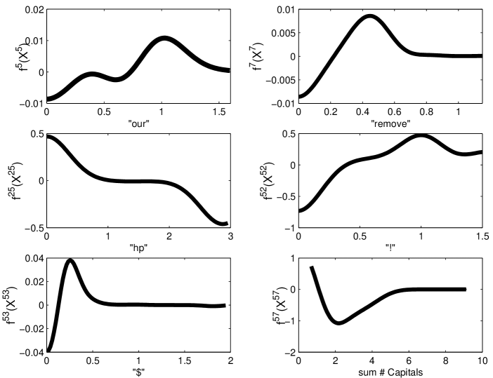
Figure 7: Results of the spam dataset. The non-sparse components as found by application of Subsection 3.3 are shown suggesting a number of usefull indicator variables for classifing a mail message as spam or non-spam. The final classifier takes the form $f(X)=f^{5}(X^{5})+f^{7}(X^{7})+f^{25}(X^{25})+f^{52}(X^{52})+f^{53}(X^{53})+f^{56}(X^{56})$ where 6 relevant components were selected out of the 56 provided indicators.

6 Conclusions

This chapter describes nonlinear additive models based on LS-SVMs which are capable of handling higher dimensional data for regression as well as classification tasks. The estimation stage results from solving a set of linear equations with a size approximatively equal to the number of training datapoints. Furthermore, the additive regularization framework is employed for formulating dedicated regularization schemes leading to structure detection. Finally, a fusion argument for component selection and structure detection based on training componentwise LS-SVMs and validation performance is introduced to improve the generalization abilities of the method. Advantages of using componentwise LS-SVMs include the efficient estimation of additive models with respect to classical practice, interpretability of the estimated model, opportunities towards structure detection and the connection with existing statistical techniques.

Acknowledgments. This research work was carried out at the ESAT laboratory of the Katholieke Universiteit Leuven. Research Council KUL: GOA-Mefisto 666, GOA AMBioRICS, several PhD/postdoc & fellow grants; Flemish Government: FWO: PhD/postdoc grants, projects, G.0240.99 (multilinear algebra), G.0407.02 (support vector machines), G.0197.02 (power islands), G.0141.03 (Identification and cryptography), G.0491.03 (control for intensive care glycemia), G.0120.03 (QIT), G.0452.04 (new quantum algorithms), G.0499.04 (Robust SVM), G.0499.04 (Statistics) research communities (ICCoS, ANMMM, MLDM); AWI: Bil. Int. Collaboration Hungary/ Poland; IWT: PhD Grants,GBOU (McKnow) Belgian Federal Science Policy Office: IUAP P5/22 (‘Dynamical Systems and Control: Computation, Identification and Modelling’, 2002-2006) ; PODO-II (CP/40: TMS and Sustainability); EU: FP5-Quprodis; ERNSI; Eureka 2063-IMPACT; Eureka 2419-FliTE; Contract Research/agreements: ISMC/IPCOS, Data4s, TML, Elia, LMS, Mastercard is supported by grants from several funding agencies and sources. GOA-Ambiorics, IUAP V, FWO project G.0407.02 (support vector machines) FWO project G.0499.04 (robust statistics) FWO project G.0211.05 (nonlinear identification) FWO project G.0080.01 (collective behaviour) JS is an associate professor and BDM is a full professor at K.U.Leuven Belgium, respectively.

References

- (1)
- Antoniadis (1997) Antoniadis, A. (1997). Wavelets in statistics: A review. Journal of the Italian Statistical Association (6), 97–144.
- Antoniadis and Fan (2001) Antoniadis, A. and J. Fan (2001). Regularized wavelet approximations (with discussion). Journal of the American Statistical Association 96, 939–967.
- Blake (1989) Blake, A. (1989). Comparison of the efficiency of deterministic and stochastic algorithms for visual reconstruction. IEEE Transactions on Image Processing 11, 2–12.
- Boyd and Vandenberghe (2004) Boyd, S. and L. Vandenberghe (2004). Convex Optimization. Cambridge University Press.
- Cressie (1993) Cressie, N. A. C. (1993). Statistics for spatial data. Wiley.
- Cristianini and Shawe-Taylor (2000) Cristianini, N. and J. Shawe-Taylor (2000). An Introduction to Support Vector Machines. Cambridge University Press.
- Donoho and Johnstone (1994) Donoho, D.L. and I.M. Johnstone (1994). Ideal spatial adaption by wavelet shrinkage. Biometrika 81, 425–455.
- Fan (1997) Fan, J. (1997). Comments on wavelets in statistics: A review. Journal of the Italian Statistical Association (6), 131–138.
- Fan and Li (2001) Fan, J. and R. Li (2001). Variable selection via nonconvex penalized likelihood and its oracle properties. Journal of the American Statistical Association 96(456), 1348–1360.
- Frank and Friedman (1993) Frank, L.E. and J.H. Friedman (1993). A statistical view of some chemometric regression tools. Technometrics (35), 109–148.
- Friedmann and Stuetzle (1981) Friedmann, J. H. and W. Stuetzle (1981). Projection pursuit regression. Journal of the American Statistical Association 76, 817–823.
- Fu (1998) Fu, W.J. (1998). Penalized regression: the bridge versus the lasso. Journal of Computational and Graphical Statistics (7), 397–416.
- Fukumizu et al. (2004) Fukumizu, K., F. R. Bach and M. I. Jordan (2004). Dimensionality reduction for supervised learning with reproducing kernel Hilbert spaces. Journal of Machine Learning Reasearch (5), 73–99.
- Gunn and Kandola (2002) Gunn, S. R. and J. S. Kandola (2002). Structural modelling with sparse kernels. Machine Learning 48(1), 137–163.
- Hastie and Tibshirani (1990) Hastie, T. and R. Tibshirani (1990). Generalized addidive models. London: Chapman and Hall.
- Hastie et al. (2001) Hastie, T., R. Tibshirani and J. Friedman (2001). The Elements of Statistical Learning. Springer-Verlag. Heidelberg.
- Linton and Nielsen (1995) Linton, O. B. and J. P. Nielsen (1995). A kernel method for estimating structured nonparameteric regression based on marginal integration. Biometrika 82, 93–100.
- MacKay (1992) MacKay, D. J. C. (1992). The evidence framework applied to classification networks. Neural Computation 4, 698–714.
- Neter et al. (1974) Neter, J., W. Wasserman and M.H. Kutner (1974). Applied Linear Statistical Models. Irwin.
- Nikolova (1999) Nikolova, M. (1999). Local strong homogeneity of a regularized estimator. SIAM Journal on Applied Mathematics 61, 633–658.
- Pelckmans et al. (2003) Pelckmans, K., J.A.K. Suykens and B. De Moor (2003). Additive regularization: Fusion of training and validation levels in kernel methods. (Submitted for Publication) Internal Report 03-184, ESAT-SISTA, K.U.Leuven (Leuven, Belgium).
- Poggio and Girosi (1990) Poggio, T. and F. Girosi (1990). Networks for approximation and learning. In: Proceedings of the IEEE. Vol. 78. Proceedings of the IEEE. pp. 1481–1497.
- Schoelkopf and Smola (2002) Schoelkopf, B. and A. Smola (2002). Learning with Kernels. MIT Press.
- Stone (1982) Stone, C.J. (1982). Optimal global rates of convergence for nonparametric regression. Annals of Statistics 13, 1040–1053.
- Stone (1985) Stone, C.J. (1985). Additive regression and other nonparameteric models. Annals of Statistics 13, 685–705.
- Suykens and Vandewalle (1999) Suykens, J.A.K. and J. Vandewalle (1999). Least squares support vector machine classifiers. Neural Processing Letters 9(3), 293–300.
- Suykens et al. (2002) Suykens, J.A.K., T. Van Gestel, J. De Brabanter, B. De Moor and J. Vandewalle (2002). Least Squares Support Vector Machines. World Scientific, Singapore.
- Tibshirani (1996) Tibshirani, R.J. (1996). Regression shrinkage and selection via the lasso. Journal of the Royal Statistical Society (58), 267–288.
- Tibshirani (1997) Tibshirani, R.J. (1997). The lasso method for variable selection in the cox model. Statistics in Medicine (16), 385–395.
- Tikhonov and Arsenin (1977) Tikhonov, A.N. and V.Y. Arsenin (1977). Solution of Ill-Posed Problems. Winston. Washington DC.
- Vapnik (1998) Vapnik, V.N. (1998). Statistical Learning Theory. John Wiley and Sons.
- Wahba (1990) Wahba, G. (1990). Spline models for observational data. SIAM.