Abstract

A review of Bayesian restoration of digital images based on Monte Carlo techniques is presented. The topics covered include Likelihood, Prior and Posterior distributions, Poisson, Binary symmetric channel and Gaussian channel models of Likelihood distribution, Ising and Potts spin models of Prior distribution, restoration of an image through Posterior maximization, statistical estimation of a true image from Posterior ensembles, Markov Chain Monte Carlo methods and cluster algorithms.

Introduction

Noise, in a digital image, is an inevitable nuisance; often it defeats the purpose, the image was taken for. Noise mars the scene it intends to depict and affects the artist in the person looking at the image; it limits the diagnosis a doctor makes from a medical image; it interferes with the inferences a physicist draws from the images acquired by his sophisticated spectrometers and microscopes; it restricts useful information that can be extracted from the images transmitted by the satellites on earth’s resources and weather; etc. Hence it is important that noise be eliminated and true image restored.

Noise, in the first place, enters a digital image while being acquired due to, for example faulty apparatus and poor statistics; it enters while storage due to aging, defects in storage devices etc.; it enters during transmission through noisy channels. We shall not be concerned, in this review, with specific details of mechanisms of noise entry and image degradation. Instead, we confine our attention mostly to de-noising, also called restoration, of digital images.

Conventional digital image processing techniques rely on the availability of qualitative and quantitative information about the specific degradation process that leads to noise in an image. These algorithms work efficiently on applications they are intended for; perhaps they would also work reasonably well on closely related applications. But they are unreliable for applications falling outside their domain. There are not many image restoration algorithms that can handle a wide variety of images. Linear filters like low pass filters, high pass filters etc., and non-linear filters like median filters, constrained least mean square filters etc., are a few familiar examples belonging to the category of general purpose algorithms.

An important aim of image restoration research is to devise robust algorithms based on simple and easily implementable ideas and which can cater to a wide spectrum of applications. It is precisely in this context, a study of the statistical mechanics of images and image processing should prove useful. The reasons are many.

1. Statistical mechanics aims to describe macroscopic properties of a material from those of its microscopic constituents and their interactions; an image is a macroscopic object and its microscopic constituents are the gray levels in the pixels of the image frame.

2. Statistical mechanics is based on a few general and simple principles and can be easily adapted to image processing studies.

3. Bayesian statistics is closely related to statistical mechanics as well as to the foundations of stochastic image processing in particular and information processing in general.

4. Several statistical mechanical models have a lot in common with image processing models.

But why should we talk of these issues now ? Notice, images have entered our personal and professional life in a big way in the recent times - personal computers, INTERNET, digital cameras, mobile phones with image acquisition and transmission capabilities, new and sophisticated medical and industrial imaging devices, spectrometers, microscopes, remote sensing devises etc..

Let me briefly touch upon a few key issues of image processing to drive home the connection between statistical mechanics and image processing. Mathematically, an image is a matrix of non-negative numbers, representing the gray levels or intensities in the pixels of an image plane. A pixel is a tiny square on the image plane and represents an element of the picture. Pixels coarse-grain the image plane. The gray level in a pixel defines the state of the pixel. Pixels are analogous to the vertices of a lattice that coarse-grain space in a statistical mechanical two dimensional model. The gray levels are analogous to the states of spins or of atoms sitting on the lattice sites. Spatial correlations in an image can be modeled by defining suitable interaction between states of two pixels, exactly like the spin-spin interaction on a lattice model. In fact one can define an energy for an image by summing over these interactions. An exponential Bayesian Prior is analogous to Gibbs distribution. It is indeed this correspondence which renders an image, a Markov random field and vice versa. We can define a Kullback-Leibler entropy distance for constructing a Likelihood probability distribution of images. Temperature, in the context of image processing, represents a parameter that determines the smoothness of an image. The energy-entropy competition, responsible for different phases of matter, is like the Prior - Likelihood competition that determines the smoothness and feature-quality of an image in Bayesian Posterior maximization algorithms. Simulated annealing that helps equilibration in statistical mechanical models has been employed in image processing by way of starting the restoration process at high temperature and gradually lowering the temperature to improve noise reduction capabilities of the chosen algorithm. Mean-field approximations of statistical mechanics have been employed for hyper-parameters estimation in image processing. In fact several models and methods in statistical mechanics have their counter parts in image processing. These include Ising and Potts spin models, random spin models, Bethe approximation, Replica methods, renormalization techniques, methods based on bond percolation clusters and mean field approximations. We can add further to the list of common elements of image processing and statistical mechanics. Suffice is to say that these two seemingly disparate disciplines have a lot to learn from each other. It is the purpose of this review to elaborate on these analogies and describe several image restoration algorithms inspired by statistical mechanics.

Image processing is a vast field of research with its own idioms and sophistication. It would indeed be impossible to address all the issues of this subject in a single review; nor are we competent to undertake such a task. Hence in this review we shall restrict attention to a very limited field of image processing namely the Bayesian de-noising of images employing Markov chain Monte Carlo methods. We have made a conscious effort to keep the level of discussions as simple as possible.

Stochastic image processing based on Bayesian methodology was pioneered by Derin, Eliot, Cristi and Gemen [1], Gemen and Gemen [2] and Besag [3]. For an early review see Winkler [4]; for a more recent review on the statistical mechanical approach to image processing see Tanaka [5]. Application of analytical methods of statistical mechanics to image restoration process can be found in [6]. The spin glass theory of statistical mechanics has been applied to information processing [7]. Infinite range Ising spin models have been applied to image restoration employing replica methods [8]. A brief account of the Bayesian restoration of digital images employing Markov chain Monte Carlo methods was presented in [9]. The present review, is essentially based on [9] with more details and examples. The review is organized as follows.

We start with a mathematical representation and a stochastic description of an image. We discuss a Poisson model for image degradation to construct a Likelihood distribution. We show how Kullback-Leibler distance emerges naturally in the context of Poisson distributions. Then we show how to quantify the smoothness of an image through an energy function. This is followed by a discussion of Ising and Potts spin Hamiltonians often employed in modeling of magnetic transitions. We define a Bayesian Prior as a Gibbs distribution. Such a description renders an image a Markov random field. Bayes’ theorem combines a subjective Prior with a Likelihood model incorporating the data on the corrupt image and gives a Posterior - a conditional distribution from which we can infer the true image. We show how the Likelihood and the Prior compete to increase the Posterior, the competition being tuned by temperature. The Prior tries to smoothen out the entire image with the Likelihood competing to preserve all the features, genuine as well as noisy, of the given image. For a properly tuned temperature the Likelihood loses on noise but manages to win in preserving image features; similarly the Prior loses on smoothening out the genuine features of the image but wins on smoothening out the noise inhomogeneities. The net result of the competition is that we get a smooth image with all genuine inhomogeneities in tact. The image that maximizes the Posterior for a given temperature provides a good estimate of the true image. We describe a simple Monte Carlo algorithm to search for the Posterior maximum and present a few results of processing of noisy toy and benchmark images.

Then we take up a detailed discussion of Markov Chain Monte Carlo methods based on Metropolis and Gibbs sampler; we show how to estimate the true image through Maximum $\grave{{\rm a}}$ Posteriori (MAP), Maximum Posterior Marginal (MPM) and Threshold Posterior Mean (TPM) statistics that can be extracted from an equilibrium ensemble populating the asymptotic segment of a Markov chain of images. We present results of processing of toy and benchmark images employing the algorithms described in the review. Finally we take up the issue of sampling from a Prior distribution employing bond percolation clusters. The cluster algorithms can be adapted to image processing by sampling cluster gray level independently from the Likelihood distribution. Cluster algorithms ensure faster convergence to Posterior ensemble from which the true image can be inferred. We employ a single cluster growth algorithm to process toy and benchmark images and discuss results of the exercise. We conclude with a brief summary and a discussion of possible areas of research in this exciting field of image processing, from a statistical mechanics point of view.

Mathematical Description of an Image

Consider a region of a plane discretized into tiny squares called picture elements or pixels for short. Let ${\cal S}$ be a finite set of pixels. For convenience of notation we identify the spatial location of a pixel in the image plane by a single index $i$. Also we say that index $i$ denotes a pixel. Mathematically, a collection $\Theta=\{\theta_{i}\ :\ i\in{\cal S}\}$ of non-negative numbers is called an image. Let $N\ <\ \infty$ denote the cardinality of the set ${\cal S}$. In other words $N$ is the number of pixels in the image plane. $\theta_{i}$ denotes the intensity or gray level in the pixel $i\in{\cal S}$. The state of a pixel is defined by its gray level. Let us denote by $\widehat{\Theta}=\{\widehat{\theta}_{i}\ :\ i\in{\cal S}\}$, the true image. $\hat{\Theta}$ is not known to us. Instead we have a noisy image $X=\{x_{i}:i\in{\cal S}\}$. The aim is to restore the true image $\hat{\Theta}$ from the given noisy image $X$.

Stochastic Description of an Image

In a stochastic description, we consider an image $\Theta$ as a collection of random variables $\{\theta_{i}\ :\ i\in{\cal S}\}$. Consider for example, $N$ pixels painted with $Q$ gray levels, $\{0,\ 1,\ \cdots,\ Q-1\}$. The gray level Label $0$ denotes black and the gray level label $Q-1$ denotes white. Each pixel can take any one of the $Q$ gray levels. Collect all the possible images you can paint, in a set, denoted by the symbol $\Omega$, called the state space. $\Omega$ is analogous to the coarse grained phase space of a classical statistical mechanical system. Let $\widehat{\Omega}$ denote the total number of images in the state space. It is clear that $\widehat{\Omega}=Q^{N}$. Both $\widehat{\Theta}$ and $X$ belong to $\Omega$. If all the images belonging to $\Omega$ are equally probable then we can resort to a uniform ensemble description.

Figure (1 : Left) depicts a $10\times 10$ image painted randomly with $5$ gray levels labeled by integers from $0$ to $4$, with the label $0$ denoting black and the label $4$ denoting white. The $10\times 10$ matrix of non-negative numbers (the gray level labels) that provides a mathematical representation of the image is also shown in Fig. (1 : Right).

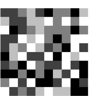
$$\ \ \ \ \ \ \ \ \ \ \ \ \ \ \ \ \ \ \ \ \ \ \ \ \ \ \ \ \ \ \ \ \ \ \ \ \ \ \ \ \ \ \ \ \ \ \ \ \ \ \ \ \ \ \ \ \ \ \ \ \ \ \ \ \ \ \ \ \begin{pmatrix}1&1&2&3&1&0&2&2&0&3\\[2.84526pt] 3&1&1&3&3&4&2&4&2&4\\[2.84526pt] 4&0&1&2&3&2&2&2&0&2\\[2.84526pt] 1&1&4&3&4&2&0&2&4&4\\[2.84526pt] 1&3&2&4&3&1&2&0&4&1\\[2.84526pt] 0&3&4&1&1&4&0&4&3&4\\[2.84526pt] 1&2&0&4&2&1&1&4&1&0\\[2.84526pt] 0&0&2&0&2&0&3&1&4&0\\[2.84526pt] 2&4&1&4&0&0&1&4&0&1\\[2.84526pt] 4&1&2&1&3&4&3&3&0&0\end{pmatrix}$$

Figure 1: (Left) A $10\times 10$ random image painted with five gray levels with $0$ representing black and $4$ representing the white. (Right) The matrix of non-negative numbers (gray levels) representing the image.

In image processing terminology, $\Theta$ is called a random field. Thus the noisy image $X$ on hand is a random field. The noisy image $X=\{x_{i}\ :\ i\in{\cal S}\}$ has

1. a systematic component representing the features of $\widehat{\Theta}$, that has survived image degradation

2. and

3. a stochastic component that accounts for the noise that enters $\widehat{\Theta}$ during degradation .

A stochastic model for $X$ is constructed by defining a conditional probability of $X|\widehat{\Theta}$ ($X$ given $\widehat{\Theta}$). This conditional probability is denoted by ${\cal L}(X|\widehat{\Theta})$ and is called the Likelihood probability distribution, or simply the Likelihood. ${\cal L}(X|\widehat{\Theta})$ can be suitably modeled to describe the stochastic degradation process that produced $X$ from $\widehat{\Theta}$.

Let us consider a simple and general model of image degradation based on Poisson statistics, which will render transparent the idea and use of likelihood distribution.

Poisson Likelihood Distribution

We consider the random field $X$ as constituting a collection of independent random variable $\{x_{i}\ :\ i\in{\cal S}\}$. We take each $x_{i}$ to be a Poisson random variable. The motivation is clear. Image acquisition is simply a counting process. Poisson process is a simple and a natural model for describing counting. There is only one parameter in a Poisson distribution, namely the mean. We take $\langle x_{i}\rangle=\widehat{\theta}_{i}$. The Likelihood of $x_{i}|\widehat{\theta}_{i}$ is given by,

$${\cal L}(x_{i}|\widehat{\theta}_{i}) = \frac{1}{x_{i}\ !}\bigg{(}\widehat{\theta}_{i}\bigg{)}^{x_{i}}\exp(-\widehat{\theta}_{i})$$ (1)

We assume $\{x_{i}\ :\ i\in{\cal S}\}$ to be independent random variables. The joint distribution is then the product of the distributions of the individual random variables. Hence we can write the Likelihood distribution of $X|\widehat{\Theta}$ as,

$${\cal L}(X|\widehat{\Theta}) = \prod_{i\in{\cal S}}{\cal L}(x_{i}|\widehat{\theta}_{i})$$ (2)

$$= \prod_{i\in{\cal S}}\frac{\bigg{(}\widehat{\theta}_{i}\bigg{)}^{x_{i}}e^{-\widehat{\theta}_{i}}}{x_{i}\ !}$$

The above Poisson Likelihood can be conveniently expressed as,

$${\cal L}(X|\widehat{\Theta}) = \exp\bigg{[}-F(\widehat{\Theta},X)\bigg{]}\ \prod_{i\in{\cal S}}\ \frac{1}{x_{i}\ !},$$ (3)

where,

$$F(\widehat{\Theta},X)=\sum_{i\in{\cal S}}\bigg{[}\widehat{\theta}_{i}-x_{i}\log(\widehat{\theta}_{i})\bigg{]}$$ (4)

The advantage of Poisson and related likelihood distributions is that there is no hyper-parameter that needs to be optimized.

Kullback-Leibler Entropy Distance

It is clear from the discussion on Poisson Likelihood that the function $F(\Theta,X)$ serves to quantify how far away is an image $\Theta$ from another image $X$. Let us investigate as to what extent does the function $F(\Theta,X)$ meet the requirements of a distance metric.

$F(\Theta,X)\neq 0$ when $\Theta=X$ and it is not symmetric in its arguments. Let us write $F(\Theta,X)$ as,

$$F(\Theta,X)=\sum_{i\in{\cal S}}f(\theta_{i},x_{i}),$$ (5)

and study the behaviour of $f(\theta_{i},x_{i})$ as a function of $\theta_{i}$ with a known value of $x_{i}$. We have,

$$f(\theta_{i};x_{i}) = \theta_{i}-x_{i}\log(\theta_{i}),$$

$$\frac{df}{d\theta_{i}} = 1-\frac{x_{i}}{\theta_{i}}.$$ (6)

It is clear from the above that,

$$\frac{df}{d\theta_{i}} = 0$$ (7)

when $\theta_{i}=x_{i}$. In other words at $\theta_{i}=x_{i}$, the function $f(\theta_{i};x_{i})$ is an extremum. To determine whether it is a minimum or a maximum we consider the second derivative of $f(\theta_{i};x_{i})$ at $\theta_{i}=x_{i}$. We have,

$$\frac{d^{2}f}{d\theta_{i}^{2}}\bigg{|}_{\theta_{i}=x_{i}} = \frac{1}{x_{i}}\ \ >\ \ 0,$$ (8)

implying that $f(\theta_{i};x_{i})$ is minimum at $\theta_{i}=x_{i}$. Let $f_{m}=x_{i}-x_{i}\log(x_{i})$ denote the minimum value of $f(\theta_{i};x_{i})$. We define a new function,

$$g(\theta_{i},x_{i}) = f(\theta_{i},x_{i})-f_{m}$$ (9)

$$= (\theta_{i}-x_{i})+(\theta_{i}-x_{i})\log(\theta_{i}/x_{i}).$$

The function $g(\theta_{i},x_{i})$ is not symmetric in its arguments. Hence we define,

$$F_{i}(\theta_{i},x_{i}) = g(\theta_{i},x_{i})+g(\theta_{i}\to x_{i},x_{i}\to\theta_{i})$$ (10)

$$= (\theta_{i}-x_{i})\log(\theta_{i}/x_{i})$$

We can now define a new distance between $\Theta$ and $X$ as

$$F(\Theta,X)=\sum_{i\in{\cal S}}(\theta_{i}-x_{i})\log(\theta_{i}/x_{i})$$ (11)

We see that that the new distance function $F(\Theta,X)=0$ when $\Theta=X$ and is positive definite when $\Theta\neq X$; also $F$ is symmetric in its arguments. We shall take $F(\Theta,X)$ as a measure of the distance between the images $\Theta$ and $X$ . $F(\Theta,X)$ is the same as the symmetric Kullback-Leibler entropy [10]. This is also called by various names like Kullback-Leibler distance, Kullback-Leibler divergence, mutual information, relative entropy etc., defined for quantifying the separation between two probability distributions. We refer to $F(\Theta,X)$ given by Eq. (11) as Kullback-Leibler distance.

Hamming Distance

Another useful function that quantifies the separation between two images $\Theta$ and $X$, defined on a common image plane, is the Hamming distance, defined as,

$$F(\Theta,X)=\sum_{i\in{\cal S}}{\cal I}(\theta_{i}\neq x_{i}),$$ (12)

where the indicator function,

$${\cal I}(\eta)=\begin{cases}1\ {\rm if\ the\ statement}\ \ \eta\ {\rm is\ true},\cr\ \ \ \cr 0\ {\rm if\ the\ statement}\ \ \eta\ {\rm is\ not\ true}.\end{cases}$$ (13)

Hamming distance simply counts the number of pixels in $\Theta$ having gray levels different from those in the corresponding pixels in $X$. The Hamming distance $F(\Theta,X)$ defined above is symmetric in its arguments; also $F(\Theta,X)=0$, when $\Theta=X$. We shall find use for Hamming distance while processing binary images or even for processing images which have a few number of gray levels. However if the number of gray levels in an image is large, then the Kullback-Leibler distance should prove more useful.

Gaussian Channel Likelihood Distribution

A popular model for image degradation is based on assuming $x_{i}$ to be Gaussian random variable with

$$\langle x_{i}\rangle = \alpha\ \widehat{\theta}_{i},$$

$$\langle x^{2}_{i}\rangle-\langle x_{i}\rangle^{2} = \sigma^{2}.$$ (14)

In the above $\alpha$ and $\sigma$ are called the hyper-parameters of the Gaussian channel model. The Likelihood of $x_{i}|\widehat{\theta}_{i}$ is given by,

$${\cal L}(x_{i}|\widehat{\theta}_{i})=\frac{1}{\sigma\sqrt{2\pi}}\ \exp\bigg{[}-\frac{1}{2\sigma^{2}}\ \Bigg{(}x_{i}-\alpha\theta_{i}\Bigg{)}^{2}\ \bigg{]}$$ (15)

We assume $\{x_{i}\ :\ i\in{\cal S}\}$ to be independent random variables. The Likelihood in the Gaussian channel model is given by,

$${\cal L}(X|\widehat{\Theta}) = \frac{1}{\Big{(}\sigma\sqrt{2\pi}\Big{)}^{N}}\exp\bigg{[}-\frac{1}{2\sigma^{2}}\sum_{i\in{\cal S}}\Big{(}x_{i}-\alpha\theta_{i}\Big{)}^{2}\bigg{]},$$ (16)

where $N$ is the total number of pixels in the image plane.

Binary Symmetric Channel Likelihood Distribution

Consider a binary image $\widehat{\Theta}$ which degrades to $X$ by the following algorithm. Take a pixel $i\in{\cal S}$ in the image plane of $\widehat{\Theta}$. Call a random number $\xi$ uniformly distributed in the unit interval. If $\xi\leq\tilde{p}$ set $x_{i}$ to the other gray level. Otherwise set $x_{i}=\widehat{\theta}_{i}$. This process is described by the Likelihood distribution given by,

$${\cal L}(x_{i}|\widehat{\theta}_{i}) = \tilde{p}\ {\cal I}(x_{i}\neq\widehat{\theta}_{i})+(1-\tilde{p})\ {\cal I}(x_{i}=\widehat{\theta}_{i})$$ (17)

It is convenient to express the above Likelihood as,

$${\cal L}(x_{i}|\widehat{\theta}_{i}) = \frac{\exp\Big{[}-\beta_{L}{\cal I}(x_{i}\neq\widehat{\theta}_{i})\Big{]}}{1+\exp(-\beta_{L})}$$ (18)

The hyper-parameter $\beta_{L}$ is related to $\tilde{p}$ as given below.

$$\tilde{p} = \frac{\exp(-\beta_{L})}{1+\exp(-\beta_{L})}$$

$$\beta_{L} = \log\Big{(}\frac{1}{\tilde{p}}-1\Big{)}$$ (19)

The procedure described above is repeated independently on all the pixels. The Likelihood of $X|\widehat{\Theta}$ is then the product of the Likelihoods of $x_{i}|\widehat{\theta}_{i}$ and is given by,

$${\cal L}(X|\widehat{\Theta}) = \frac{\exp\Big{[}-\beta_{L}F(X,\widehat{\Theta})\Big{]}}{\sum_{X}\exp\Big{[}-\beta_{L}F(X,\widehat{\Theta})\Big{]}},$$ (20)

where $F(X,\widehat{\Theta})$ is the Hamming distance between $X$ and $\widehat{\Theta}$. The hyper-parameter $\beta_{L}=1/T_{L}$ can be interpreted as inverse temperature of the degradation process. When $T_{L}=0$ we have $\tilde{p}=0$. In other words at $T_{L}=0$ no degradation takes place and $X=\widehat{\Theta}$. As $T_{L}$ increases the noise level increases. When $T_{L}=\infty$, we have $\tilde{p}=0.5$ and the image $X$ i becomes completely random. In other words each pixel can have independently a black or white gray level with equal probability.

Degradation of a Multi-Gray Level Image

Consider an image $\widehat{\Theta}$ painted with $Q$ gray levels with labels $0,\ 1,\ 2,\ \cdots,\ Q-1$. The label $0$ denotes black and the label $Q-1$ denotes white. Let us say that the degradation of $\widehat{\Theta}$ to $X$ proceeds as follows. Take a pixel $i\in{\cal S}$. Call a random number $\xi$ uniformly distributed in the range $0$ to $1$. If $\xi\leq\tilde{p}$, then select one of the $Q-1$ gray levels (excluding $\widehat{\theta}_{i}$) randomly and with equal probability and assign it to $x_{i}$. Otherwise set $x_{i}=\widehat{\theta}_{i}$. This process of degradation is described by the Likelihood given by,

$${\cal L}(x_{i}|\widehat{\theta}_{i}) = \tilde{p}\ {\cal I}(x_{i}\neq\widehat{\theta}_{i})+(1-\tilde{p})\ {\cal I}(x_{i}=\widehat{\theta}_{i})$$ (21)

It is convenient to express the above Likelihood as,

$${\cal L}(x_{i}|\widehat{\theta}_{i}) = \frac{\exp\Big{[}-\beta_{L}{\cal I}(x_{i}\neq\widehat{\theta}_{i}\Big{]}}{1+(Q-1)\exp(-\beta_{L})}.$$ (22)

The hyper-parameter $\beta_{L}$ is related to $\tilde{p}$ as given below,

$$\tilde{p} = \frac{\exp(-\beta_{L})}{1+(Q-1)\exp(-\beta_{L})}$$

$$\beta_{L} = \log\Big{[}(Q-1)(\frac{1}{\tilde{p}}-1)\Big{]}.$$ (23)

The degradation process described above is repeated independently on all the pixels. Then the Likelihood of $X|\widehat{\Theta}$ is the product of the Likelihoods of $x_{i}|\widehat{\theta}_{i}$ and is given by,

$${\cal L}(X|\widehat{\Theta}) = \frac{\exp\Big{[}-\beta_{L}F(X,\widehat{\Theta})\Big{]}}{\sum_{X}\exp\Big{[}-\beta_{L}F(X,\widehat{\Theta})\Big{]}},$$ (24)

where $F(X,\widehat{\Theta})$ is the Hamming distance between $X$ and $\widehat{\Theta}$. The hyper-parameter $\beta_{L}=1/T_{L}$ can be interpreted as inverse temperature of the degradation process. When $T_{L}=0$ we have $\tilde{p}=0$ indicating no degradation and $X=\widehat{\Theta}$. As $T_{L}$ increases the noise level increases. When $T_{L}=\infty$, we have $\tilde{p}=1-(1/Q)$ which tends to unity when $Q\to\infty$. In all the above if substitute $Q=2$ we recover the results of binary symmetric channel degradation.

Three Ingredients of Bayesian Methodology

In a typical image processing algorithm, we start with an initial image $\Theta_{0}$. A good choice is $\Theta_{0}=X$, the given noisy image. We generate a chain of images

$$\Theta_{0}\to\Theta_{1}\to\Theta_{2}\cdots\to\Theta_{n}\to\Theta_{n+1}\to$$ (25)

by an algorithm and hope that a suitably defined statistics over the ensemble of images in the chain would approximate well the original image $\widehat{\Theta}$. In constructing a chain of images we shall employ Bayesian methodology.

The first ingredient of a Bayesian methodology is the Likelihood which models the degradation of $\widehat{\Theta}$ to $X$. We have already seen a few models of image degradation. The second ingredient is an $\grave{{\rm a}}$ priori distribution, simply called a Prior, denoted by $\pi(\Theta)$. The Prior is a distribution of gray levels on ${\cal S}$. The choice of a Prior is somewhat subjective. The third ingredient is an $\grave{{\rm a}}$ posteriori distribution or simply called Posterior, denoted by the symbol $\pi(\Theta|X)$. Posterior is a conditional distribution; it is the distribution of $\Theta|X$.

Bayesian $\grave{{\rm{\bf a}}}$ Priori Distribution

As we said earlier, the choice of a Prior in Bayesian methodology is subjective. The Prior should reflect what we believe a clean image should look like. We expect an image to be smooth. We say that a pixel is smoothly connected to its neighbour if the gray levels in them are the same. Smaller the difference between the gray levels, smoother is the connection. This subjective belief is encoded in a Prior as follows.

We introduce an interaction energy between the states of two pixels. We confine the interaction to nearest neighbour pixels. Thus the states of a pair $i,j$ of nearest neighbour pixels interact with an energy denoted by $E_{i,j}$. We take the interactions to be pair-wise additive and define an energy of the image $\Theta$ as,

$$E(\Theta) = \sum_{\langle i,j\rangle}E_{i,j}(\Theta).$$ (26)

In the above, the symbol $\langle i,j\rangle$ denotes that the pixels $i$ and $j$ are nearest neighbours and the sum is taken over all distinct pairs of nearest neighbour pixels in the image plane. We model $E_{i,j}$ in such a way that it is small when the gray levels are close to each other and large when the gray levels differ by a large amount. Thus, a smooth image has less energy. We define the Prior as,

$$\pi(\Theta) = \frac{1}{Z(\beta)}\exp\Big{[}-\beta_{P}E(\Theta)\Big{]}$$ (27)

where $\beta_{P}=1/T_{P}$ and $T_{P}$ is a smoothening parameter called the Prior temperature. $Z(\beta_{P})$ is the normalization constant and is given by,

$$Z(\beta_{P}) = \sum_{\Theta}\exp\Big{[}-\beta_{P}E(\Theta)\Big{]}.$$ (28)

The Prior, as defined above, is called the Gibbs distribution. Such a definition of Prior  implies that $\Theta$ is a Markov random field. Conversely if $\Theta$ is a Markov random field, then its Prior can be modeled as a Gibbs distribution.

Markov Random Field

A Markov Random field generalizes the notion of a discrete time Markov process, or also called a Markov chain. Appendix (2) briefly describes a general as well as a time homogeneous or equilibrium Markov chain. A sequence of random variables, parametrized by time and obeying Markovian dependence, constitutes a Markov chain. Instead of time we can use spatial coordinate as parameter to describe the chain, in one dimensional setting. The concept of Markov random field extends Markovian dependence from one dimension to a general setting [11]

In a Markov random field $\Theta$, the state of a pixel is at best dependent on the state of the pixels in its neighbourhood. Accordingly, let $i\in{\cal S}$ be a pixel and let $\nu_{i}$ denote the set of pixels that form the neighbourhood of $i$. Let ${\cal N}=\{\nu_{i}\ :\ i\in{\cal S}\}$ denote a neighbourhood system for ${\cal S}$. In other words, ${\cal N}$ is any collection of subsets of ${\cal S}$ for which,

1. $i\notin\nu_{i}$

2. $i\in\nu_{j}\Longleftrightarrow j\in\nu_{i}$.

The pair $\{{\cal S},{\cal N}\}$ is a graph. An image $\Theta$ is a Markov random field if

$$\pi\Big{(}\theta_{i}\Big{|}\{\theta_{j}\ :\ j\neq i;j\in{\cal S}\}\Big{)}=\pi\Big{(}\theta_{i}\Big{|}\{\theta_{j}\ :\ j\in\nu_{i}\}\Big{)}\ \forall\ i\in{\cal S}.$$ (29)

From the definition of conditional probability in terms of joint probability, we have,

$$\pi(\Theta) = \pi(\theta_{1},\theta_{2},\cdots,\theta_{N})$$ (30)

$$= \pi\Big{(}\theta_{i}\Big{|}\big{\{}\theta_{j}:j\neq i;j\in{\cal S}\big{\}}\Big{)}\pi(\theta_{j}:j\neq i;j\in{\cal S})\ \ \forall\ \ i\in\ {\cal S}$$

Since $\Theta$ is a Markov random field, the above can be written as,

$$\pi(\Theta)=\pi\Big{(}\theta_{i}\Big{|}\big{\{}\theta_{j}:j\in\nu_{i}\big{\}}\Big{)}\pi(\theta_{j}:j\neq i;j\in{\cal S})\ \forall\ i\in{\cal S}.$$ (31)

Iterating alternately, we get,

$$\pi(\Theta)=\prod_{i\in{\cal S}}\ \pi\Big{(}\theta_{i}\Big{|}\big{\{}\theta_{j}:j\in\nu_{i}\big{\}}\Big{)}.$$ (32)

Let us define,

$$U_{i}(\Theta)=-\log\pi\Big{(}\theta_{i}\Big{|}\{\theta_{j}:j\in\nu_{i}\}\Big{)},$$ (33)

and

$$U(\Theta)=\sum_{i\in{\cal S}}U_{i}(\Theta).$$ (34)

Then,

$$\pi(\Theta)=\frac{1}{Z}\exp\big{[}-U(\Theta)\big{]},$$ (35)

where $Z$ is the normalization constant. This expression for the Prior is identical to the Gibbs distribution if we identify $U(\Theta)=\beta_{P}E(\Theta)$ and $Z$ as the $Z(\beta_{P})$, defined in Eq. (28). Note that $E(\Theta)$ is a sum of the interaction energies of the states of nearest neighbour pixels and hence is consistent with the Markov random field requirement. It is important that the interaction must be restricted to a finite range for $\Theta$ to be a Markov random field. Since we consider in this review only nearest neighbour interactions, this condition is automatically satisfied.

The equivalence of Gibbs distribution in statistical mechanics and Markov random field in spatial statistics was established, see [12, 13] following the work of Hammersley and Clifford [14].

Ising Model for $\grave{{\rm{\bf a}}}$ Priori Distribution

Ising model [15] is the simplest and perhaps the most studied of models in statistical mechanics. Let us consider a Prior inspired by Ising model. We consider an image having only two gray levels, designated as say $\zeta=1,\ 3$ or equivalently $S=\pm 1$; we have the transformation $\zeta=S+2$. The index $\zeta=1$ ($S=-1$) refers to black and $\zeta=2$ ($S=+1$) refers to white gray level. The interaction energy of the states of two nearest neighbour pixels $i$ and $j$ is given by,

$$E_{i,j}(\Theta) = {\cal I}(\theta_{i}\neq\theta_{j}).$$ (36)

It is clear that if the two pixels have the same gray level, the interaction energy is zero. If their gray levels are different the interaction energy is unity. In the language of the physicists, the ground state of the two-pixel system has zero energy and the excited state has unit energy. The two energy levels are separated by $\Delta E=1$. The energy of an Ising image $\Theta$ is given by,

$$E(\Theta)=\sum_{\langle i,j\rangle}E_{i,j}(\Theta)=\sum_{\langle i,j\rangle}{\cal I}\left(\theta_{i}\neq\theta_{j}\right).$$ (37)

The Ising Prior can be written as,

$$\pi(\Theta) = \frac{1}{Z(\beta_{P})}\exp\Big{[}-\beta_{P}\sum_{\langle i,j\rangle}{\cal I}(\theta_{i}\neq\theta_{j})\Big{]}$$ (38)

where $Z(\beta_{P})$ is the canonical partition function. Ising Prior in conjunction with Hamming Likelihood is suitable for restoring binary images.

Potts Model for $\grave{{\rm{\bf a}}}$ Priori Distribution

Potts model [16] is an important lattice model in which there are discrete number of states at each site. Consider a multiple gray level image. The gray levels are taken as $\{0,\ 1,\ 2,\ \cdots,Q-1\}$. We have then a $Q$ state Potts model. The label $0$ denotes black, and the label $Q-1$ denotes white gray levels. The different shades correspond to the intermediate Potts numbers. The expressions for the energy associated with the states of two nearest neighbour pixels, for the Potts Hamiltonian and for the Potts Prior are the same as the ones defined for the Ising model given in the last section. Potts Prior in conjunction with Hamming or Kullback-Leibler Likelihood is suitable for restoring images painted with a small number of gray levels.

Gemen-McClure Model for $\grave{{\rm{\bf a}}}$ Priori Distribution

Gemen and McClure[17] recommended a Prior in which the states of two neighbouring pixels interact with an energy given by,

$$E_{i,j}(\Theta)=-\frac{1}{1+C(\theta_{i}-\theta_{j})^{2}},$$ (39)

where $C$ is a hyper-parameter that determines the width of the distribution. The value of $E_{i,j}(\Theta)$ ranges from a minimum of $-1$ when $|\theta_{i}-\theta_{j}|=0$ to a maximum of $0$, when $|\theta_{i}-\theta_{j}|\to\infty$. Gemen-McClure interaction potential is depicted in Fig. (2) for $C=0.1,\ 1.0,\ {\rm and}\ 10.0$. The function $E_{i,j}(\Theta)$ is symmetric about $|\theta_{i}-\theta_{j}|=0$ and its width decreases with increase of $C$. For large $C$ the Gemen-McClure interaction reduces to an Ising interaction with ground state energy at $-1$ and excited state energy at $0$. The Gemen-McClure Prior is thus given by,

$$\pi(\Theta)=\frac{1}{Z(\beta_{P})}\ \exp\bigg{[}\ -\beta_{P}\ \sum_{\langle i,j\rangle}\ \frac{-1}{1+C\ (\ \theta_{i}-\theta_{j}\ )^{2}\ }\bigg{]}$$ (40)

where $Z(\beta_{P})$ is the partition function that normalizes the Prior.

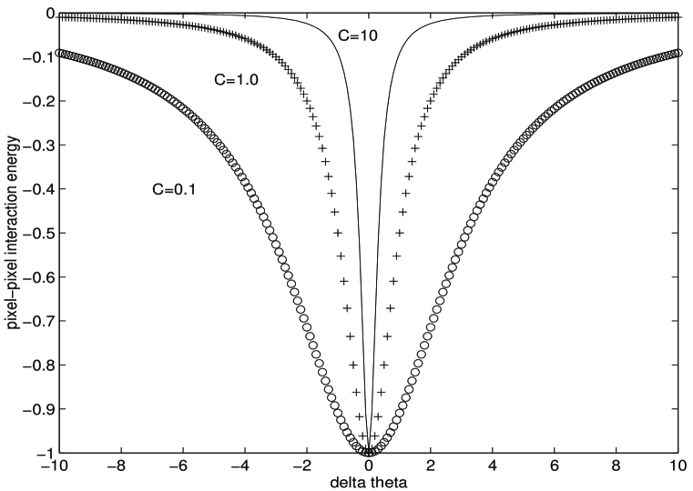
Figure 2: Gemen-McClure energy $E_{i,j}$ versus $|\theta_{i}=\theta_{j}|$ for $C=0.1,1.0,10.0$; when $C$ increases the width of the function decreases. In the limit $C\to\infty$ the Gemen-McClure model reduces to the Ising model with ground state at $-1$ and excited state at $0$.

Relation between $\beta_{P}$ and $\widehat{\Theta}$

It is clear from the discussion above that the hyper-parameter $\beta_{P}$ will depend on the smoothness and features present in $\widehat{\Theta}$. The Prior is given by,

$$\pi(\widehat{\Theta}) = \frac{1}{Z(\beta_{P})}\exp\Big{[}-\beta_{P}E(\widehat{\Theta})\Big{]},$$ (41)

where $Z(\beta_{P})$ is the partition function,

$$Z(\beta_{P})=\sum_{\widehat{\Theta}}\exp\Big{[}-\beta_{P}E(\widehat{\Theta})\Big{]}$$ (42)

The value of $\beta_{P}$ is implicitly given by the relation below.

$$\langle E\rangle = -\frac{\partial}{\partial{\beta_{P}}}\log\Big{[}Z(\beta_{P})\Big{]}$$ (43)

Consider for example the Ising/Potts Priors. The energy of $\widehat{\Theta}$ is completely determined by the number of pairs of nearest neighbour pixels with dis-similar gray levels. In the graph theoretic language two nearest neighbour pixels are separated by an edge. Let $N_{E}$ denote the total number of edges in image plane of $\widehat{\Theta}$. If two nearest neighbour pixels have the same gray levels then we say the edge separating them is a satisfied bond. Let $B(\widehat{\Theta})$ denote the number of satisfied bonds in the image $\widehat{\Theta}$. In other words $B$ is the number of nearest neighbour pairs of similar pixels. We see immediately that $E(\widehat{\Theta})=N_{E}-B$. Thus the value of the hyper-parameter $\beta_{L}$ can in principle be calculated from the values of $N_{E}$ and $B$ of a given image $\widehat{\Theta}$.

Bayesian $\grave{{\rm{\bf a}}}$ Posteriori Distribution

The Posterior distribution in the Bayesian methodology is given by the product of the Likelihood and the Prior. This is called Bayes’ theorem, discussed for e.g. in [18, 19]. Appendix 1 states Bayes’ theorem.

According to Bayes’ theorem,

$$\pi(\Theta|X)=\frac{{\cal L}(X|\theta)\pi(\theta)}{\sum_{\Theta}{\cal L}(X|\theta)\pi(\theta)}.$$ (44)

The Bayesian Posterior can be formally written as,

$$\pi(\Theta|X)=\frac{\exp\bigg{[}-\bigg{\{}\beta_{L}F(\Theta,X)+\beta_{P}E(\Theta)\bigg{\}}\bigg{]}}{\sum_{\Theta}\exp\bigg{[}-\bigg{\{}\beta_{L}F(\Theta,X)+\beta_{P}E(\Theta)\bigg{\}}\bigg{]}}.$$ (45)

It is convenient to work in terms of intensive quantities. To this end we define $E$ per pair of nearest neighbour pixels and $F$ per pixel. Accordingly we divide energy by, $N_{E}$, the number of nearest neighbour pairs of pixels in the image plane. For an $L\times L$ pixel image, we have $N_{E}=2L(L-1)\approx 2L^{2}({\rm for\ large\ }L)$. We divide $F(\Theta,X)$ by $L^{2}$. In the expression for the Posterior above, the argument of the exponential function can be viewed as a weighted sum of $F(\Theta,X)$ and $E(\Theta)$. The weight attached to $E$ is $\beta_{P}$ and the weight attached to the $F$ is $\beta_{L}$. The relevant quantity is the relative weights attached to $F$ and $E$. Hence we set $\beta_{L}=1$ and $\beta_{P}=\beta$, where $\beta$ is the value of $\beta_{P}$ measured in units of $\beta_{L}$. Also, it is convenient to work with normalized weights and accordingly we divide the whole exponent by $1+\beta$. The final expression for the Posterior that we use in the image restoration algorithm is given by

$$\pi(\Theta|X)=\frac{\exp\bigg{[}-L^{-2}(1+\beta)^{-1}\Big{\{}F(\Theta,X)+2^{-1}\beta E(\Theta)\Big{\}}\bigg{]}}{\sum_{\Theta}\exp\bigg{[}-L^{-2}(1+\beta)^{-1}\Big{\{}F(\Theta,X)+2^{-1}\beta E(\Theta)\Big{\}}\bigg{]}}.$$ (46)

The advantage of the above expression is there is only one parameter $\beta=1/T$ that needs to be tuned for good image restoration.

Bayesian Maximum $\grave{{\rm{\bf a}}}$ Posteriori (MAP)

The aim of image restoration is to construct the true image $\widehat{\Theta}$ from the given noisy image $X$. The simplest estimate of $\widehat{\Theta}$ is the image which maximizes the Posterior.

For a given temperature, the Posterior increases when $F(\Theta,X)$ decreases. In other words closer $\Theta$ is to $X$, larger is the value of $\pi(\Theta|X)$. Though $X$ is corrupt, it is the best we have and we would like to retain during image-restoration process as many features of $X$ as possible.

The Posterior increases when $E$ decreases for a given temperature $T$. In other words smoother $\Theta$ is, larger is the value of $\pi(\Theta|X)$. Thus, there is a Prior-Likelihood competition, the Prior trying to smoothen the image and the Likelihood trying to keep the image as close to $X$ as possible. In other words the Prior tries to make all the pixels acquire the same grave level and the Likelihood tries to bind the image to the data $X$. As a result we get an image which has in it the features of $X$ (because of competition from the Likelihood) and which is smooth with out noise (because of competition from the Prior). The nature of Prior-Likelihood competition is tuned by Temperature, see below. What happens when the temperature $T$ is large ? Temperature determines the relative competitiveness of the Likelihood and Prior toward increasing the Posterior. For a given $T$,

1. the relative weight attached to $F(\Theta,X)$ is $T/(1+T)$, and

2. the relative weight attached to $E$ is $1/(1+T)$.

When $T$ is large, feature - retention (i.e. the Likelihood) is given more importance. However if $T$ is very large, the image restoration algorithm would interpret even the noise in $X$ as a feature and retain it; as a result the restored image would be noisy. What happens when the temperature $T$ is small ? When $T$ is small, smoothening (i.e. the Prior) is given more importance. However if $T$ is too small, there is a danger: the image restoration algorithm would misinterpret even genuine inhomogeneities and fine features of $X$ as noise and eliminate them.

Best image restoration is expected over an intermediate range of $T$, often obtained by trial and error. The problem of image restoration is thus reduced to a problem of sampling, independently and randomly with equal probabilities, a large number of images from the state space $\Omega$. These images constitute a microcanonical ensemble. Calculate the Posterior of each member of the microcanonical ensemble. Pick up the image which gives the highest value of the Posterior and call it $\Theta_{{\rm MAP}}$; the suffix MAP stands for the Maximum $\grave{{\rm a}}$ Posteriori. $\Theta_{{\rm MAP}}$ is called an MAP estimate of $\widehat{\Theta}$. We can also employ other statistics, defined over the state space $\Omega$, to estimate $\widehat{\Theta}$, see below.

Maximum $\grave{{\rm{\bf a}}}$ Posteriori Marginal (MPM)

We partition the state space $\Omega$ into mutually exclusive and exhaustive subsets as described below. Consider a pixel $i\in{\cal S}$. Define $\Omega^{(i)}_{\zeta}$ as a subset of images for which the gray level of the pixel $i$ is $\zeta$, where $\zeta\in\{0,\ 1,\ \cdots Q-1\}$.

$$\Omega^{(i)}_{\zeta}=\bigg{\{}\Theta\in\Omega,\ \theta_{i}(\Theta)=\zeta\bigg{\}}\ \ {\rm for}\ \ \zeta=0,1,\cdots Q-1$$ (47)

Calculate now marginal Posteriors,

$$\pi^{(i)}_{\zeta}=\sum_{\Theta\ \in\ \Omega^{(i)}_{\zeta}}\pi(\Theta|X)\ \ \ {\rm for}\ \ \ \zeta=0,1,\cdots Q-1\ .$$ (48)

Thus we get an array of $Q$ marginals $\Big{\{}\pi^{(i)}_{\zeta}:\zeta=0,1,\cdots Q-1\Big{\}}$. We define

$$\zeta^{(i)}_{{\rm MPM}} = {\rm arg}\begin{subarray}{\ }\cr\ \cr\ {\rm{max}}\cr\ \ \zeta\end{subarray}\ \ \pi^{(i)}_{\zeta}$$ (49)

which stands for the value of $\zeta$ that maximizes the function $\pi^{(i)}_{\zeta}$. In other words, $\zeta^{(i)}_{{\rm MPM}}$ denotes the value of the gray level for which the marginal Posterior is maximum. Repeat the above for all the pixels in the image plane, and obtain a collection of numbers that represents an approximation to $\widehat{\Theta}$:

$$\Theta_{{\rm MPM}}=\Big{\{}\zeta^{(i)}_{{\rm MPM}}:i\in{\cal S}\Big{\}}.$$ (50)

$\Theta_{{\rm MPM}}$ is called a Maximum $\grave{{\rm a}}$ Posteriori (MPM) estimate of $\widehat{\Theta}$.

Threshold $\grave{{\rm{\bf a}}}$ Posteriori Mean (TPM)

Calculate an average image, $\overline{\Theta}=\{\overline{\theta}_{i}\ :\ i\in{\cal S}\}$, where,

$$\overline{\theta_{i}}=\sum_{\Theta\in\Omega}\theta_{i}(\Theta)\ \pi(\Theta|X)\ \ \forall\ \ i\ \ \in\ \ {\cal S}.$$ (51)

We define,

$$\zeta^{(i)}_{{\rm TPM}} = {\rm arg}\begin{subarray}{\ }\cr\ \cr\ {\rm{min}}\cr\ \ \zeta\end{subarray}\ \ \Big{[}\zeta-\sum_{\Theta\in\Omega}\theta_{i}(\Theta)\pi(\Theta|X\Big{]}^{2}$$ (52)

which stands for the value of $\zeta$ that minimizes $[\zeta-\sum_{\Theta\in\Omega}\theta_{i}(\Theta)]^{2}$. In other words $\zeta^{(i)}_{{\rm TPM}}$ is the value of $\zeta$ closest to $\overline{\theta_{i}}$. Carry out the above exercise for all the pixels in the image, and get a collection of gray levels that represents an approximation to $\widehat{\Theta}$:

$$\Theta_{{\rm TPM}}=\Big{\{}\zeta^{(i)}_{{\rm TPM}}:i\in{\cal S}\Big{\}}.$$ (53)

$\Theta_{{\rm TPM}}$ is called Threshold $\grave{{\rm a}}$ Posteriori Mean (TPM) estimate of $\widehat{\Theta}$. It is easily seen that for a binary image $\Theta_{{\rm TPM}}=\Theta_{{MPM}}$.

Elements of Digital Image Restoration

A typical image restoration process is depicted in Fig. (3). We represent the unknown true image by $\widehat{\Theta}$, which gets corrupted to $X$. The degradation of $\widehat{\Theta}$ to $X$ is modeled by the Likelihood ${\cal L}(X|\widehat{\Theta})$. Bayes theorem helps synthesize the Likelihood (available in the form of a degradation model and data on the corrupt image $X$) with a Prior (that models your subjective beliefs about true image). The result is a Posterior $\pi(\Theta|X)$. An ensemble of images having the Posterior distribution is shown as $\Theta$ in Fig. (3). From this Posterior ensemble we can make MAP, MPM and TPM estimates of the true image.

Figure 3: Digital image restoration : $\widehat{\Theta}$ denotes the true image (first square in the top row) which gets corrupted to $X$ (second square in the top row). The degradation of $\widehat{\Theta}$ to $X$ is modeled by ${\cal L}(X|\widehat{\Theta})$. Bayes theorem helps construct a Posterior $\pi(\Theta|X)$ from the Likelihood and a Prior. A Posterior ensemble of images ( set of squares in the right end of top row). MAP, MPM and TPM estimates of $\widehat{\Theta}$ (depicted by the three squares in the second row) are made from the Posterior ensemble. See [6]

Algorithm for Calculating ${\mathbf{\Theta}_{{\rm{\textbf{M}AP}}}}$

A straight forward procedure to calculate $\Theta_{{\rm MAP}}$ is to attach a Posterior probability to each image belonging to the state space $\Omega$ and pick up that image which has a maximum Posterior probability. This is easily said than done. Note that the number of images belonging to state space $\Omega$ is $Q^{N}$. Let us consider a small, say $10\times 10$ binary image ($Q=2$). The number of pixels is thus $100$. Then $\widehat{\Omega}=2^{100}\approx 10^{30}$. Calculating the Posteriors for these $10^{30}$ images is an impossible task even on the present day high speed computers. A simple procedure would be to sample randomly and with equal probability a certain large number of images in the neighbourhood of the given image $X$; these images constitute a microcanonical ensemble. Find the image, in the microcanonical ensemble, that maximizes the Posterior and recommend it as an MAP estimate of $\widehat{\Theta}$. An algorithm for doing this is described below.

Fix the temperature. Start with an image $\Theta_{0}=X$. Call this the current image. i.e. $\Theta_{C}=\Theta_{0}$

1. Calculate $\pi_{C}=\pi(\Theta_{c}|X)$.

2. Select a pixel, say $j$, randomly from the image plane.

3. Switch the gray level of the pixel $j$ from its current value to a value sampled randomly and with equal probability from the gray level labels
   $\zeta=\{0,\ 1,\ \cdots~{},\ Q-1\}$.

4. Calculate $\pi_{t}=\pi(\Theta_{t}|X)$.

5. If $\pi_{t}>\pi_{C}$, then accept the trial image and set $\Theta_{1}=\Theta_{t}$; otherwise $\Theta_{1}=\Theta_{0}$.

6. Take $\Theta_{1}$ as the current image $\Theta_{C}$,

7. go to step (1).

Iterate the whole process several times. A set of $N$ update attempts constitutes an iteration. Collect the images at the end of each iteration. Thus we get a sequence of images with monotonically non-decreasing Posteriors. Asymptotically we get $\Theta_{{\rm MAP}}$, called an MAP estimate of $\widehat{\Theta}$.

How does Posterior maximization lead to image restoration ?

A simple explanation of how does a Bayesian Posterior maximization lead to de-noising is depicted in Fig. (4) and described below.

Figure 4: Local region of $\Theta_{C}$ is depicted at Left. The gray level label of the central pixel is switched from $1$ to $3$ and a trial image $\Theta_{t}$ is constructed. The corresponding local region of $\widehat{\Theta}_{t}$ is depicted at Right. This move leads to local smoothening of the image. Let us assume that the sub-image depicted at Left belongs to $X$ and that depicted at Right belongs to $\widehat{\Theta}$. Then the above move increases $F$ by one unit and decreased $E$ by $4$ units. The Posterior increases if $T<2$. In other words Prior wins over Likelihood if $T_{L}\ <\ 2$, leading to de-noising.

Consider a local region of the current image $\Theta_{C}$ having a pixel $m$ with gray level label $1$ and with all its four nearest neighbours having gray level label $3$. Let us denote by the symbol $\nu$ the set of five pixels : the pixel $m$ and its four nearest neighbours. Let us say that in $\widehat{\Theta}$, the pixels belonging to $\nu$ have all the same gray level $3$ and hence is smooth locally. It is the process of degradation that has to led to the noise inhomogeneity in the pixel $m$. We have,

$$F(\Theta_{C},X) = \sum_{i\notin\nu}{\cal I}\Big{(}\theta_{i}(\Theta_{C})\neq x_{i}\Big{)}+\sum_{i\in\nu}{\cal I}\Big{(}\theta_{i}(\Theta_{C})\neq x_{i}\Big{)}$$ (54)

Let us denote the first term in the above sum (over pixels not belonging to $\nu$) as $F_{0}$. The second term is zero since $\theta_{i}(\Theta_{C})=x_{i}(X)\ \forall\ i\in\nu$. We get $F(\Theta_{C},X)=F_{0}$. Similarly,

$$E(\Theta_{C}) = \sum_{\begin{subarray}{\ }\langle i,j\rangle\cr i\neq m\end{subarray}}{\cal I}\Big{(}\theta_{i}(\Theta_{C})\neq\theta_{j}(\Theta_{C})\Big{)}+\sum_{\begin{subarray}{\ }\langle i,j\rangle\cr i=m\end{subarray}}{\cal I}\Big{(}\theta_{i}(\Theta_{C})\neq\theta_{j}(\Theta_{C})\Big{)},$$ (55)

where $\langle i,j\rangle$ denotes that $i$ and $j$ are nearest neighbour pixels and the sum extends over all distinct nearest neighbour pairs of pixels. Let us denote by $E_{0}$ the first term in the above. The second term is $4$ since there are four dis-similar nearest neighbour pairs of pixels in the sub-image $\nu$. Hence $E(\Theta_{C})=E_{0}+4$. In the simulation, we change the gray level of pixel $m$ from it present value of $1$ to $3$ and call the resulting image as $\Theta_{t}$. We find that $F(\Theta_{t},X)=F_{0}+1$ and $E(\Theta_{t})=E_{0}.$ Eventhough the move increases $F$ by one unit, it decreases $E$ by four units. Let the Posteriors of $\Theta_{C}$ and $\Theta_{t}$ be denoted by $\pi_{C}$ and $\pi_{t}$ respectively. The ratio of the Posteriors can be calculated and is given by,

$$\frac{\pi_{t}}{\pi_{C}}=\exp\bigg{[}-\frac{1}{L^{2}(1+\beta)}\ \Big{(}1-2\beta\Big{)}\bigg{]}$$ (56)

which is greater than unity whenever $\beta\ >\ (1/2)$ or $T\ <\ 2$. Since we accept $\Theta_{t}$ only when $\pi_{t}$ is greater than $\pi_{C}$, de-noising takes place when $T<2$.

It is clear from the discussion above, that removal of an inhomogeneity entails energy reduction. Hence a Prior tries to remove all inhomogeneities in the image plane including the genuine ones. On the other hand, the Likelihood binds the image to the data $X$. It tries to retain all the features of $X$ including the inhomogeneities that have their origin in noise. It is the temperature that tunes the competition between the Prior and the Likelihood.

Restoration of Toy Images

Binary Robot

We have created a $92\times 92$ binary image $\widehat{\Theta}$, referred to as ROBOT, depicted in Fig. (5 : Left). To corrupt a binary image with noise we proceed as follows. We select a pixel $i$ and change the gray level label from its present value to the other with a probability $0.05$: Call a random number $\xi$; if $\xi\leq 0.05$, change the gray level. Otherwise do not change the gray level. Carry out this exercise on all the pixels independently. This is equivalent to adding $5\%$ noise to the image; there is no spatial correlations in the noise added. The resulting corrupt image, called $X$ is depicted in Fig. (5 : Middle). Employing Ising Prior and Hamming Likelihood we have calculated an MAP estimate of $\widehat{\Theta}$ at $T=0.51$ depicted in Fig. (5 : Right).

Five-gray Level Robot

We have constructed a $5$ gray level ROBOT image on a $56\times 56$ image frame depicted in Fig. (6 : Left). We corrupt the image with $5\%$ noise and get $X$ depicted in Fig. (6 : Middle). Employing Potts Prior and Hamming Likelihood we have made an MAP estimate of the true image which is depicted in Fig. (6 : Right). The image restoration has been carried out at $T=0.51$. We monitored the Bayesian Posterior maximum at the end of each iteration. The Posterior maximum is a monotonically non-decreasing of the iteration index. Eventually the Posterior maximum saturates as shown in Fig. (7).

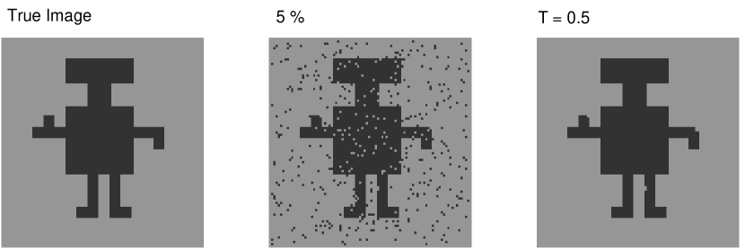
Figure 5: Binary ROBOT image; $L=92$. (Left) true image $\hat{\Theta}$ (Middle) Image $X$ constructed by adding noise to $\widehat{\Theta}$, as described in the section  ‘Binary Symmetric Channel Likelihood distribution’with $\tilde{p}=0.05$ and (Right) Restored image, $\Theta_{{\rm MAP}}$. Complete restoration happens after one iteration. Image restoration has been carried out at $T=0.5$

MAP estimates of the 5-gray level Potts image made at a high temperature ($T=2.5$) and at a low temperature $0.01$ and at intermediate temperature ($T=0.51$) are shown in Fig. (8); the high temperature $\Theta_{{\rm MAP}}$ is noisy and the low temperature $\Theta_{{\rm MAP}}$ has several of its fine features distorted. Good image restoration obtains for temperatures in the neighbourhood of $0.5$.

Restoration of Benchmark Images

Binary Lena Image

We have taken a benchmark image called the Lena, painted with 256 gray levels. We have converted it to a binary image and is displayed in Fig. (9 : Left). We introduce $5\%$ noise and the resulting image $X$ is also shown in Fig. (9 : Middle). We have employed Ising Prior and Hamming distance and made an MAP estimate of the original image. The restored image $\Theta_{{\rm MAP}}$ is depicted in Fig. (9 Right).

We have processed the same image at temperatures $T=0.1,\ 1.1,\ 2.5$ and the results are displayed in Fig. (10). At $T=0.1$, the algorithm has removed all the fine features of the image. At $T=2.5$ the algorithm has interpreted even noise as features and retained them. Good image restoration seems to happen at temperatures between $1$ and $1.5$

Five and Ten Gray Level Lena Images

We have coarse grained the same Lena image to $5$ gray levels and the result is shown in Fig. (11 : Left). The image corrupted with $5\%$ noise is depicted in Fig. (11 : Middle) and an MAP estimate made with Potts Prior and Hamming distance is depicted in Fig. (11 : Right).

Results of image restoration of Lena image with $10$ gray levels are shown in Fig. (12). It is clear from the discussions above such a search algorithm would be time consuming. It would be advantageous to obtain an ensemble of images which has the desired Posterior distribution so that the required statistics can be calculated by simple arithmetic averaging over the Posterior ensemble.

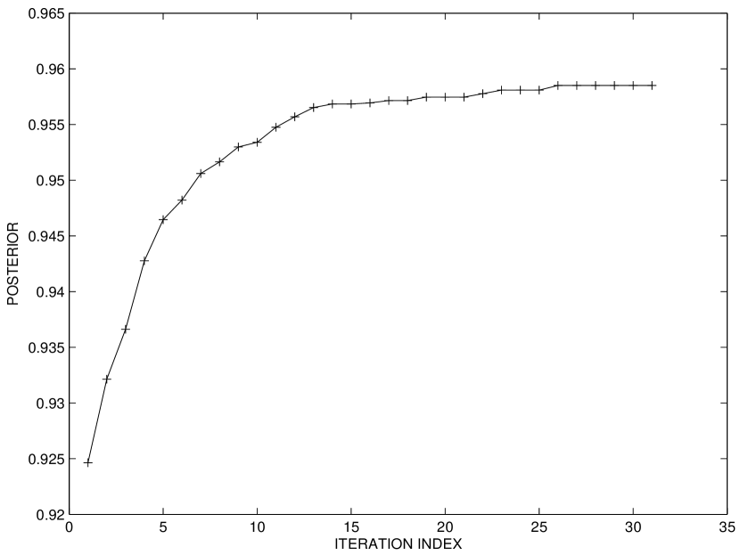
Figure 6: ROBOT image: L=56; $5$ gray levels; Image restoration has been carried out employing Potts Prior, Hamming Likelihood. (Left) True image $\widehat{\Theta}$ (middle) Image $X$ constructed by adding noise to $\widehat{\Theta}$, as described in the section  ‘Degradation of a multi-gray level image’ with $\tilde{p}=.05$, and (right) restored image $\Theta_{{\rm MAP}}$ at $T=0.51$.

Figure 7: Posterior maximum versus iteration index, for image restoration shown in Fig. (6)

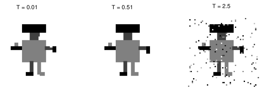
Figure 8: Robot image: $L=56$; $5$ gray levels. Image restoration employs Potts Prior and Hamming Likelihood. The Maximum $\grave{{\rm{\bf a}}}$ Posteriori (MAP) estimates at low : $T=.01$ (Left), intermediate $T=0.51$ (middle) and high : $T=2.5$ (right) temperatures are depicted.

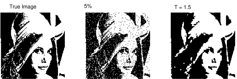
Figure 9: Restoration of the benchmark binary Lena image, employing Ising Prior and Hamming Posterior. $L=141$ (Left) True image $\hat{\Theta}$ (Middle) Image $X$ constructed by adding noise to $\widehat{\Theta}$ as described in section  ‘Binary Symmetric Channel Likelihood distribution’  with $\tilde{p}=.05$. (Right) Restored image, $\Theta_{{\rm MAP}}$ after one iteration. image processing has been carried out at temperature $T=1.5$

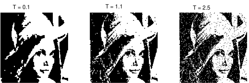
Figure 10: Restoration of binary Lena image at three temperatures. MAP estimates of $\widehat{\Theta}$ are given. (Left) $T=0.1$ (Middle) $T=1.1$ and (Right) $T=2.5$. $\widehat{\Theta}$ and $X$ are the same ones depicted in Fig. (9).

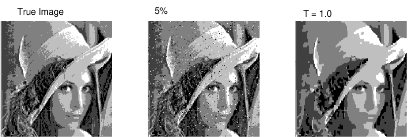
Figure 11: Restoration of the benchmark 5-gray level Lena image employing Potts Prior and Hamming distance. (Left) True image $\widehat{\Theta}$ (Middle) Image $X$ constructed by adding noise to $\widehat{\Theta}$ as described in section  ‘Degradation of a multi-gray level image’ with $\tilde{p}=0.05$. The image restoration was done at T=1.0

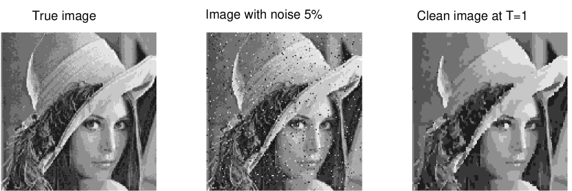
Figure 12: Restoration of the benchmark 10-gray level Lena image employing Potts Prior and Hamming distance. (Left) True image $\widehat{\Theta}$ (Middle) Image $X$ constructed by adding noise to $\widehat{\Theta}$ as described in section  ‘Degradation of a multi-gray level image’ with $\tilde{p}=0.05$. The image restoration was done at T=1.0

It is precisely in this context that the Metropolis algorithm[20], discovered for purpose of obtaining a canonical ensemble of microstates in statistical mechanics becomes useful. We outline below a Markov chain Monte Carlo technique in conjunction with the Metropolis algorithm and its variant, to obtain a Posterior ensemble of images.

Markov Chain Monte Carlo for Sampling from $\grave{{\rm{\bf a}}}$ Posteriori Distribution

Monte Carlo is a numerical technique that makes use of random numbers to solve a problem. Historically, the first large scale Monte Carlo work carried out dates back to the middle of twentieth century. This work pertained to simulation of neutron multiplication, scattering, streaming and eventual absorption in a medium or escape from it. Application of Monte Carlo method to problems in statistical mechanics started with the discovery of the Metropolis algorithm [20] which generates a Markov chain of microstates converging to the desired ensemble. There exist a vast body of literature on Monte Carlo technique. We refer to [22, 23, 24, 25, 26, 27, 28, 29] for some of them. Monte Carlo constitutes a natural numerical technique for image processing. We describe below a Markov Chain Monte Carlo algorithm for image restoration.

We fix the temperature $T$. We start with an arbitrary image $\Theta_{0}$. A good choice of $\Theta_{0}$ is $X$. Then we construct a Markov chain whose asymptotic segment contains images belonging to the desired Posterior ensemble at the chosen temperature. In a Markov chain $\Theta_{0}\to\Theta_{1}\to\cdots\to\Theta_{n}\to\cdots$, the image $\Theta_{k+1}$ depends only on $\Theta_{k}$ and not on the previous history. In Appendix 2 we have described briefly, the basic elements of a Markov chain and its construction by Monte Carlo algorithms. For a detailed description of Markov chain see [31]. Here we describe only the operational details of a Markov chain Monte Carlo algorithm.

First calculate the Posterior, $\pi(\Theta_{k}|X)$ (upto a normalization constant) of the current image $\Theta_{k}$; denote it by the symbol $\pi_{k}$. Select randomly a pixel from the image plane. Change its gray level randomly, and get a trial image $\Theta_{t}$. Calculate the Posterior of the trial image, $\pi(\Theta_{t}|X)$ and denote it by $\pi_{t}$. Accept the trial image with a probability ${\hat{p}}$ given by,

$$\hat{p}={\rm min}\Big{(}1,\ \frac{\pi_{t}}{\pi_{k}}\Big{)}$$ (57)

This is called the Metropolis algorithm [20]. This is also known as Metropolis-Hastings algorithm in image processing literature. We notice that the Metropolis acceptance is based on the ratios of the Posteriors. The normalization constants cancel. Hence it is adequate if we know the Posterior upto a normalization constant.

We can also employ Gibbs’ sampler in which the acceptance probability is given by

$$\hat{p}=\frac{\pi_{t}}{\pi_{k}+\pi_{t}}.$$ (58)

The acceptance/rejection step is implemented as follows. We call a random number $\xi$, distributed uniformly in the range zero to unity. If $\xi\leq{\hat{p}}$, accept the trial image and set $\Theta_{k+1}=\Theta_{t}$. Otherwise reject the trial image and set $\Theta_{k+1}=\Theta_{k}$. Repeat the above on the image $\Theta_{k+1}$. Iterate and construct a Markov chain of images given by

$$\Theta_{0}\to\Theta_{1}\to\Theta_{2}\to\cdots\to\Theta_{n}\to\Theta_{n+1}\to\cdots$$ (59)

In practice, we define a consecutive set of $N$ attempted updates (successful or otherwise) as constituting a Monte Carlo Sweep (MCS), where $N$ is the total number of pixels in the image being processed. We take the image at the end of successive MCS and construct a Markov chain. We have shown in Appendix 2 that the asymptotic part of the chain $\{\Theta_{m}\ :\ m\geq n\to\infty\}$ contains images that belong the desired Posterior ensemble. Let $\Gamma$ denote the set of images taken from the asymptotic segment of the Markov chain. $\Gamma$ is called the Posterior ensemble. Let $\widehat{\Gamma}$ denote the total number of images in $\Gamma$. MAP, MPM and TPM estimates of $\widehat{\Theta}$ can be made from the Posterior ensemble $\Gamma$ as follows.

$$\Theta_{{\rm MAP}}={\rm arg}\ \begin{subarray}{\ }\cr\ \cr{\rm max}\cr\Theta\in\Gamma\end{subarray}\ \ \pi(\Theta|X)$$ (60)

For calculating MPM estimate, we partition $\Gamma$ into mutually exclusive and exhaustive subsets of images as described below. Consider a pixel $i\in{\cal S}$. Define $\Gamma_{\zeta}^{(i)}$ as a subset of images for which the gray level of pixel $i$ is $\zeta$, where $\zeta=0,1\cdots Q-1$:

$$\Gamma_{\zeta}^{(i)}=\Big{\{}\Theta\in\Gamma,\theta_{i}(\Theta)=\zeta\Big{\}}\ {\rm for}\ \zeta=0,1,\cdots,Q-1$$ (61)

Let $\widehat{\Gamma}_{\zeta}^{(i)}$ denote the number of images belonging to the subset $\Gamma_{\zeta}^{(i)}$. Then we have,

$$\zeta_{{\rm MPM}}^{(i)} = {\rm arg}\ \begin{subarray}{\ }\cr\ \cr{\rm max}\cr\ \ \zeta\end{subarray}\ \ \widehat{\Gamma}_{\zeta}^{(i)}$$ (62)

$$\zeta_{{\rm TPM}}^{(i)} = {\rm arg}\ \begin{subarray}{\ }\cr\ \cr{\rm min}\cr\ \zeta\end{subarray}\ \bigg{[}\zeta-\frac{1}{\widehat{\Gamma}}\sum_{\Theta\in\Gamma}\theta_{i}(\Theta)\bigg{]}^{2}$$ (63)

In other words, $\zeta_{{\rm MPM}}^{(i)}$ is the value of $\zeta$ for which $\widehat{\Gamma}_{\zeta}^{(i)}$ is maximum, while $\zeta_{{\rm TPM}}^{(i)}$ is the value of $\zeta$ closest to $\overline{\theta}_{i}$ - the arithmetic average of the gray level of pixel $i$ taken over images belonging to the Posterior ensemble $\Gamma$. We depict in Fig. (13) MAP, MPM and TPM estimates for a binary ROBOT image with $L=56$.

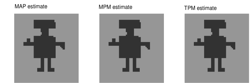
Figure 13: Image restoration employing Ising Prior, Hamming Likelihood and Markov Chain Monte Carlo with Metropolis acceptance. MAP (Left), MPM (middle) and TPM (Right) estimates made at $T=0.5$ are shown. These statistics have been obtained from the ensemble of images sampled employing Markov chain Monte Carlo in conjunction with the Metropolis algorithm. The $\Theta_{{\rm{\bf MAP}}}$ obtained from an earlier Monte Carlo search algorithm was taken as input to avoid removing initial images from the Markov chain for purpose of equilibration. All the three estimates give identical results. In any case for binary image one can show that by definition MPM and TPM estimates are the same

We have not presented in this review detailed results on the MPM and TPM estimates of the true image, because we find that these estimates are not good if we have only a single hyper-parameter in the image restoration algorithm We find that retaining two independent hyper-parameters one from the Likelihood model of degradation ($\beta_{L}$) and the other from the Prior model of out subjective expectation ($\beta_{P}$) would be required for a meaningful estimate of $\widehat{\Theta}$ through MPM and TPM statistics employing Markov chain Monte Carlo technique in conjunction with Metropolis algorithm or Gibbs sampler. We need to consider images that are consistent and that are not consistent with the Likelihood and Prior model assumptions and investigate the performance of Markov chain Monte Carlo restoration algorithms. Work in this direction is in progress and would be communicated soon.

In the Metropolis or the Heat-bath algorithms described above, only a single pixel is updated at a time. For restoring a large image, single pixel update algorithms can be frustratingly time consuming. Also if there are strong correlations in an image, which often is the case, we could think of updating the states (gray levels) of a large cluster of pixels, to speed up the algorithm. If we take an arbitrary cluster of pixels of the same gray level and update their gray levels coherently, most often the trial image constructed would get rejected in the Metropolis step. Hence it important to have a correct definition of a cluster. It is in this context a study of the cluster algorithm proposed by Swendsen and Wang [36] becomes relevant.

Swendsen-Wang Cluster Algorithm

Swendsen and Wang [36] derived an ingenious cluster algorithm for mapping the Ising/Potts spin problem to a bond-percolation problem based on the work of Kasteleyn and Fortuin [37] and Coniglio and Klein [38]. The algorithm was originally intended for overcoming the problem of critical slowing down near second-order phase transition. This algorithm has been adapted to several problems in image processing since recent times. A comparison of Swendsen-Wang algorithm and Gibbs sampler was reported in [39]. The dynamics of Swendsen-Wang algorithm in image segmentation has been investigated in [40]. Swendsen-Wang algorithm has found applications in Bayesian variable selection particularly for problems where there are multi-colinearities amongst predictors [41]. Very recently a version of Swendsen-Wang algorithm for removing Poisson noise from medical images was proposed [42]. In fact it has been recognized that the Swendsen-Wang algorithm is a particular example of a more general auxiliary variable method pioneered by Edwards and Sokal [43] and Besag and Green [44]. For a review of auxiliary variable method see [45].

Auxiliary Bond Variables

Let us first consider sampling of images from the Ising/Potts Prior. Introduce a collection ${\mathbf{\epsilon}}$, of binary random variables : ${\mathbf{\epsilon}}=\{\epsilon_{i,j}:i,j\in{\cal S}\}$ where $i,j$ are nearest neighbour pixels. These are called auxiliary bond random variables. $\epsilon_{i,j}=0\ \ {\rm or}\ \ 1$. If $\theta_{i}=\theta_{j}$ then we say there exists a satisfied bond between $i$ and $j$. A satisfied bond may be occupied ($\epsilon_{i,j}=1$) or may not be occupied ($\epsilon_{i,j}=0$). If $\theta_{i}\neq\theta_{j}$ then there is no bond connecting the pixels $i$ and $j$. In other words $\epsilon_{i,j}=0$, if $\theta_{i}\neq\theta_{j}$. Let $p$ denote the probability of occupying a satisfied bond in $\Theta$. The probability of not occupying a satisfied bond is $q=1-p$, so that $p+q=1$. We do not yet know the value of $p$ we must use for obtaining an ensemble of images distributed as per the Ising/Potts Prior. We shall take up this question after going through the following preliminaries.

Conditional, Joint and Marginal Priors

Construction of a bond structure on the given image, described above, can be expressed mathematically as,

$$\pi(\epsilon_{i,j}=1|\theta_{i}=\theta_{j}) = p,$$

$$\pi(\epsilon_{i,j}=0|\theta_{i}=\theta_{j}) = q,$$

$$\pi(\epsilon_{i,j}=1|\theta_{i}\neq\theta_{j}) = 0,$$

$$\pi(\epsilon_{i,j}=0|\theta_{i}\neq\theta_{j}) = 1.$$ (64)

The conditional Prior in terms of $p$ and $q$ is given by,

$$\pi(\epsilon|\Theta)=\prod_{\langle i,j\rangle}\bigg{[}\bigg{\{}q\ {\cal I}(\epsilon_{i,j}=0)+p\ {\cal I}(\epsilon_{i,j}=1)\bigg{\}}{\cal I}(\theta_{i}=\theta_{j})+{\cal I}(\epsilon_{i,j}=0)\ {\cal I}(\theta_{i}\neq\theta_{j})\bigg{]}.$$ (65)

The joint Prior is given by,

$$\pi(\Theta,{\mathbf{\epsilon}})=\frac{1}{Z_{1}}\prod_{\langle i,j\rangle}\bigg{[}q\ {\cal I}(\epsilon_{i,j}=0)+p\ {\cal I}(\epsilon_{i,j}=1)\ {\cal I}(\theta_{i}=\theta_{j})\bigg{]}.$$ (66)

where $Z_{1}$ is the normalization constant. From the joint Prior $\pi(\Theta,\epsilon)$, we can derive an expression for the marginal Prior $\pi(\theta)$ and is given by

$$\pi(\Theta) = \sum_{\epsilon}\pi(\Theta,\epsilon)$$

(67)

$$= \frac{1}{Z_{1}}\prod_{\langle i,j\rangle}\Big{[}p{\cal I}(\theta_{i}=\theta_{j})\ +\ q\Big{]}$$

What is the value of $p$ appropriate for sampling from the Ising/Potts Prior ? Let us start with the Ising/Potts Prior given by Eq. (38) and express it in a different form as described below.

$$\pi(\Theta) = \frac{1}{Z(\beta)}\ \exp\Big{[}-\beta\sum_{\langle i,j\rangle}{\cal I}(\theta_{i}\neq\theta_{j})\Big{]}$$

$$= \frac{1}{Z(\beta)}\ \prod_{\langle i,j\rangle}\Big{[}{\cal I}(\theta_{i}=\theta_{j})+e^{-\beta}{\cal I}(\theta_{i}\neq\theta_{j})\Big{]}$$

$$= \frac{1}{Z(\beta)}\ \prod_{\langle i,j\rangle}\Big{[}{\cal I}(\theta_{i}=\theta_{j})+\Big{\{}1-{\cal I}(\theta_{i}=\theta_{j})\Big{\}}\times e^{-\beta}\Big{]}$$

(68)

$$= \frac{1}{Z(\beta)}\ \prod_{\langle i,j\rangle}\Big{[}\big{(}1-e^{-\beta}\big{)}{\cal I}(\theta_{i}=\theta_{j})+\exp(-\beta)\Big{]}$$

Comparing the above with the marginal Prior $\pi(\Theta|\epsilon)$ given by Eq. (Conditional, Joint and Marginal Priors) we can conclude that $p=1-\exp(-\beta)$, $q=\exp(-\beta)$ and the Ising/Potts partition function $Z(\beta)$ is the same as the normalization constant of the joint Prior $Z_{1}$.

Another way of looking at the same thing, which gives a better insight into the Swendsen-Wang algorithm, is as follows. Let $N_{E}$ denote the total number of distinct nearest neighbour pairs of pixels in the image plane. If a pixel is considered as a vertex, then $N_{E}$ is the number of edges in the graph. Let $B$ denote the total number of like pairs of pixels in an image $\Theta$; i.e. $B$ is the total number of satisfied bonds in $\Theta$. The Ising/Potts Prior can be written in terms of $N_{E}$ and $B$ as follows. Consider Eq. (38). The summation in the exponent of the Ising/Potts Prior can be split into a sum over like pairs and a sum over unlike pairs,

$$\sum_{\langle i,j\rangle}{\cal I}(\theta_{i}\neq\theta_{j}) = \sum_{\begin{subarray}{\ }\langle i,j\rangle\cr\theta_{i}=\theta_{j}\end{subarray}}{\cal I}(\theta_{i}\neq\theta_{j})+\sum_{\begin{subarray}{\ }\langle i,j\rangle\cr\theta_{i}\neq\theta_{j}\end{subarray}}{\cal I}(\theta_{i}\neq\theta_{j})$$

(69)

$$= N_{E}-B$$

Thus we get,

$$\pi(\Theta) = \frac{1}{Z(\beta)}\exp\big{[}-\beta(N_{E}-B)\big{]}$$ (70)

Let $b$ denote the number of occupied bonds in the image $\Theta$. Note that $b$ is a random variable. For an image $\Theta$, the value of $b$ can range from $0$ to $B$. It is easily seen that the joint Prior $\pi(\Theta,\epsilon)$ can be expressed in terms of $N_{E}$ and $b$ as,

$$\pi(\Theta,{\mathbf{\epsilon}})=\frac{1}{Z_{1}}q^{N_{E}-b}p^{b}$$ (71)

Integrate $\pi(\Theta,{\bf\epsilon})$ over ${\bf\epsilon}$ (keeping in mind that we need to sum over the distribution of $b$) and get the marginal distribution of $\Theta$ in terms of $N_{E}$ and $B$:

$$\pi(\Theta) = \frac{1}{Z_{1}}\ \sum_{b=0}^{B}\ \frac{B!}{b!\ (B-b)!}\ q^{N_{E}-b}\ p^{b}$$

$$= \frac{1}{Z_{1}}\ q^{N_{E}-B}\ \sum_{b=0}^{B}\ \frac{B!}{b!\ (B-b)!}\ q^{B-b}\ p^{b}$$

(72)

$$= \frac{1}{Z_{1}}\ q^{N_{E}-B}$$

The above is the same as the Ising/Potts Prior given by Eq. (70), if we identify that $Z_{1}=Z(\beta)$, $q=\exp(-\beta)$ and hence $p=1-\exp(-\beta)$. We also could have come to the same conclusion directly from the marginal Prior given by Eq. (Conditional, Joint and Marginal Priors),

$$\pi(\Theta)=\frac{1}{Z_{1}}\ (p+q)^{B}\ q^{N_{E}-B}\ =\ \frac{1}{Z_{1}}\ q^{N_{E}-B}.$$ (73)

Conditional $\grave{{\rm{\bf a}}}$ Priori Distribution $\pi(\Theta|\epsilon)$

For practical implementation of the algorithm, we need conditional Priors: $\pi(\epsilon|\Theta)$ and $\pi(\Theta|\epsilon)$. The simulation strategy is to sample alternately from these two conditional Priors and construct a Markov chain of images which asymptotically converges to the Prior ensemble. We already have an expression for $\pi(\epsilon|\Theta)$ given by Eq. (65), with $q=\exp(-\beta)$ and $p=1-\exp(-\beta)$.

To derive an expression for the conditional Prior $\pi(\Theta|\epsilon)$, we proceed as follows. We have,

$$\pi(\Theta|\epsilon) = \frac{\pi(\Theta,\epsilon)}{\pi(\epsilon)}$$

$$= \frac{Z_{1}^{-1}\prod_{\langle i,j\rangle}\Big{[}q\ {\cal I}(\epsilon_{i,j}=0)+p\ {\cal I}(\epsilon_{i,j}=1){\cal I}(\theta_{i}=\theta_{j})\Big{]}}{Z_{1}^{-1}\Big{(}\prod_{\begin{subarray}{\ }\ \langle i,j\rangle\cr\epsilon_{i,j}=0\end{subarray}}\ \ q\Big{)}\Big{(}\prod_{\begin{subarray}{\ }\ \langle i,j\rangle\cr\epsilon_{i,j}=1\end{subarray}}\ \ p\Big{)}Q^{N_{C}(\epsilon)}}$$

(74)

$$= \frac{1}{Q^{N_{C}(\epsilon)}}$$

where $N_{C}$ is the number of clusters generated by imposing $\epsilon$ bonds on the image. Essentially we have converted an interacting system into a non interacting cluster system. Each cluster acts independently. We switch the gray level of each cluster of pixels randomly, coherently and independently.

Sampling $\epsilon$ from $\pi(\epsilon|\Theta_{k})$

Let $\Theta_{k}$ denote the current image in the Markov chain. Take a pixel $i$; this constitutes a single-pixel cluster. Let $\nu_{i}$ denote the set of pixels that are nearest neighbours of $i$. Take a pixel $j\in\nu_{i}$. If $\theta_{j}(\Theta_{k})\neq\theta_{i}(\Theta_{k})$ do not put a bond between them. On the other hand if $\theta_{j}(\Theta_{k})=\theta_{i}(\Theta_{k})$ we say there exists a satisfied bond between the two pixels. Then call a random number $\xi$. If $\xi\leq p=\exp(-\beta)$ then put a bond between them. In other words we occupy the satisfied bond with a probability $p$. If the decision is to occupy the satisfied bond then add the pixel to the cluster and form a two-pixel cluster. Repeat the above on all the nearest neighbours of $i$ and on all the nearest neighbours of pixels that get added to the cluster. The cluster growth will eventually terminate. Thus we get a cluster grown from the seed pixel $i$ and let us denote the cluster by the symbol $c_{1}$. . Start with a new pixel that does not belong to $c_{1}$. Grow a cluster in the region of the image plane excluding the one occupied by $c_{1}$. Call this cluster $c_{2}$. The process of growing cluster from new seeds would eventually stop when all the pixels in the image plane have been assigned with one cluster label or other. Thus we have non-overlapping and exhaustive set of clusters on the image plane.

Sampling $\Theta$ from $\pi(\Theta|\epsilon)$

Change the gray levels of all pixels in a cluster to a gray level randomly chosen from amongst the $Q$ gray levels. Carry out this process on each cluster independently. Remove the bonds in the resulting image and call it $\Theta_{k+1}$.

Construction of Prior Ensemble

Start with $\Theta_{0}=X$. Form clusters on the image plane, by sampling $\epsilon$ from $\pi(\epsilon|\Theta_{k})$ as described above. Get a new image $\Theta_{1}$ by sampling from $\pi(\Theta|\epsilon)$ as described above. Iterate and get a Markov chain of images. The asymptotic part of the Markov chain would contain images belonging to the Prior ensemble.

Next, we turn our attention to adapting the Swendsen-Wang algorithm to image restoration wherein we need to sample images from the Posterior and not from the Prior. The key point is that having formed clusters on the image plane of $\Theta_{k}$ we can get $\Theta_{k+1}$ by sampling the cluster gray levels from the Likelihood distribution independently. The whole procedure is described below.

Posterior Ensemble: Swendsen-Wang Algorithm

Start with an arbitrary image $\Theta_{0}$. A good choice is $\Theta_{0}=X$. Sample bond variables $\epsilon$ from the conditional Prior $\pi(\epsilon|\Theta_{0})$ as described earlier. We get clusters of pixels.

Consider one of the clusters, say the $k$-th cluster. Let $\eta_{k}$ denote the pixels belonging to the cluster. Sample a gray level for this cluster from the Likelihood distribution,

$$p_{\zeta} = {\cal L}\Big{(}\{\theta_{i}=\zeta\ :\ i\in\eta_{k}\}\Big{|}\{x_{i}\ :\ i\in\eta_{k}\}\Big{)},$$ (75)

$$= \frac{\exp\Big{[}-\sum_{i\in\eta_{k}}f_{i}(\theta_{i}=\zeta,x_{i})\Big{]}}{\sum_{\zeta=1}^{Q}\exp\Big{[}-\sum_{i\in\eta_{k}}f_{i}(\theta_{i}=\zeta,x_{i})\Big{]}}.$$

Sampling from the discrete distribution $\{p_{\zeta}\ :\ \zeta=0,\ 1,\ \cdots,\ Q-1\}$ is carried out as follows. Calculate the cumulative distribution

$$P_{0} = 0$$

$$P_{k} = \sum_{m=1}^{k}p_{m}$$

$$P_{Q} = 1$$ (76)

Let $\xi$ be a random number uniformly distributed between $0$ and $1$. The gray level $k$ for which $P_{k}\ <\ \xi\ \leq\ P_{k+1}$ is assigned to the pixels in the chosen cluster. Repeat the exercise for all the clusters independently. Remove the bonds. The resulting image $\Theta_{1}$ is the image for the next graph construction. Iterating we get a Markov chain,

$$\Theta_{0}\ \to\ (\Theta_{0},\epsilon_{0})\ \to\ (\Theta_{1},\epsilon_{0})\ \to\ \Theta_{1}\ \to\ (\Theta_{1},\epsilon_{1})\ \to\ (\Theta_{2},\epsilon_{1})\ \to\ \Theta_{2}\cdots\ \to\$$

$$\to \Theta_{n}\ \to\ (\Theta_{n},\epsilon_{n})\ \to\ (\Theta_{n+1},\epsilon_{n})\ \to\ \Theta_{n+1}\ \to\ \ \cdots$$

which converges asymptotically to the to the Posterior ensemble. We can make an MAP, an MPM or a TPM estimate the true image $\widehat{\Theta}$ from the Posterior ensemble.

Posterior Ensemble: Wolff’s Algorithm

Wolff [46] proposed a simple modification to the Swendsen-Wang cluster algorithm. Wolff’s cluster algorithm can be adapted to image restoration as described below.

A single cluster is grown from a randomly chosen pixel employing Swendsen-Wang prescription. The gray level of all the pixels in that cluster is updated by sampling from the Likelihood distribution. This results in a new image that constitutes the next entry in the Markov chain. A pixel is chosen randomly in the new image and the whole process is repeated. A Markov chain of images is constructed. The asymptotic part of the Markov chain would contain images that belong to the desired Posterior ensemble. An estimate of $\widehat{\Theta}$ can be made from the Posterior ensemble employing MAP or MPM or TPM statistics.

We have employed Wolff’s cluster algorithm in restoration of a binary and a $5$-gray level ROBOT image, at $T=0.51$. The results are depicted in Figures (14) and (15).

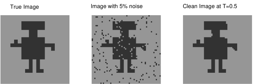
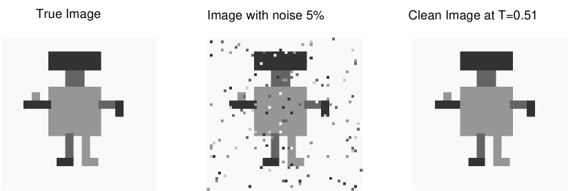
Figure 14: Image restoration employing Ising Prior, Hamming Likelihood and Wolff cluster algorithm for estimating $\Theta_{{\rm MAP}}$, for a binary ROBOT image. (Left) $\widehat{\Theta}$ (middle) $X$ (Right) MAP estimate. image processing has been carried out at temperature $T=0.5$

Figure 15: Image restoration employing Potts ($5$ gray levels) Prior, Hamming Likelihood and Wolff cluster algorithm for estimating $\Theta_{{\rm MAP}}$, for a ROBOT image. (Left) $\widehat{\Theta}$ (middle) $X$ (Right) MAP estimate. image processing has been carried out at temperature $T=0.5$

Discussions

We have presented a brief review of Markov chain Monte Carlo methods for restoration of digital images. There are three stages. The first consists of modeling of the degradation process by a conditional distribution called the Likelihood. The data on the given corrupt image is incorporated in the Likelihood. The second stage consists of constructing $\grave{{\rm a}}$ priori distribution. Our expectations of how a true image should look like are modeled in the Prior. Bayes theorem combines the likelihood and the Prior into a Posterior. The third stage consists of sampling images from the Posterior distribution, and making a statistical estimate of the true image. This is where Monte Carlo methods come in.

We have described Likelihoods based on Poisson model, Kullback-Leibler entropy distance, Hamming distance, binary symmetric channel and Gaussian channel. The Prior model discussed include Ising and Potts spin. We have given a simple explanation of how does a Posterior maximization lead to image restoration and described a Monte Carlo algorithm that does this.

Metropolis algorithm and Gibbs sampler are elegant techniques for sampling images from a Posterior distribution. The strategy is to start with a guess image and generate a Markov chain of images. We take a time homogeneous Markov transition matrix that obeys detailed balance with respect to the desired Posterior distribution. Detailed balance ensures asymptotic convergence of the Markov chain to the Posterior ensemble. Both Metropolis and Gibbs sampler obey detailed balance condition. The topics of general Markov chain, time homogeneous Markov chain, Markov transition matrix, balance equations, balance and detailed balance conditions, asymptotic convergence, time reversal of Markov chain, etc were discussed in the Appendix 2. In the main text, the steps involved in the implementation of Markov chain Monte Carlo algorithm were presented.

Then we took up the issue of cluster algorithms often employed in the context of second order phase transition. Cluster algorithms give you images that belong to the Prior ensemble. To generate a Posterior ensemble, we sample the gray level of all the pixels in a cluster randomly and independently from the Likelihood distribution. We have described Swendsen-Wang and Wolff cluster algorithms.

We can say that the techniques of simulating a canonical ensemble in statistical mechanics including cluster algorithms have been adapted to stochastic image restoration, with a reasonably good measure of success. Recently, in statistical mechanics, non-Boltzmann ensembles like multicanonical or entropic ensembles [47, 48, 49], have become popular. An advantage of such non-Boltzmann sampling techniques is that from a single simulation we can get information over a wide range of temperature by suitable reweighting schemes. The microstates that occur rarely in a canonical ensemble would occur as often as any other microstates in a multi canonical or entropic ensemble. The important point is that the multicanonical and entropic sampling Monte Carlo were intended for overcoming the problem of super-critical slowing down in first order transition. In the context of image restoration the transition from Prior dominated phase to Likelihood dominated phase is first order [6]. Hence we contend that multicanonical/entropic sampling would have a potential application in image restoration. Work in this direction is in progress and would be reported soon.

Investigating algorithms based on invasion percolation [50, 51, 52] and probability changing clusters [53, 54] may also prove useful in image restoration. The reference noisy image $X$ acts as an inhomogeneous external field. This is analogous to an Ising magnetic system in which the transition becomes first order due to presence of external field. It would be interesting to develop cluster algorithms that incorporate the presence of external fields in statistical mechanical models and adapt them to image processing. Also in stochastic image processing, ideas from random field Ising models may prove useful.

We can add to the list further. But then we stop here. We conclude by saying that analogy between image processing and statistical mechanics is rich and exploring common elements of these two disciplines should help toward developing efficient image processing algorithms.

Appendix 1

A Quick Look at Bayes’ Theorem

Figure 16: Illustration of Bayes’ theorem

Consider mutually exclusive and exhaustive events $\Theta,\ \Theta^{(1)},\ \Theta^{(2)}$.
We have,

$$\Theta\cap\Theta^{(1)}=\Theta\cap\Theta^{(2)}=\Theta^{(1)}\cap\Theta^{(2)}=\phi$$

and

$$\Theta\cup\Theta^{(1)}\cup\Theta^{(2)}\ =\Omega.$$

Let $X\subset\Omega$. We have,

$${\rm{\it Prior}} : \pi(\Theta)\ \ \ \ \ \ \ \ \ \$$

$${\rm{\it Posterior}} : \pi(\Theta|X)$$

$${\rm{\it Likelihood}} : {\cal L}(X|\Theta)$$

$${\cal L}(X|\Theta) = \frac{{\cal P}(X\bigcap\Theta)}{\pi(\Theta)}$$

$$\pi(\Theta|X) = \frac{{\cal P}(X\bigcap\Theta)}{P(X)}$$

$$= \frac{{\cal L}(X|\Theta)\pi(\Theta)}{P(X)}$$

$$P(X)={\cal L}(X|\Theta)\pi(\Theta)+{\cal L}(X|\Theta^{(1)})\pi(\Theta^{(1)})+{\cal L}(X|\Theta^{(2)})\pi(\Theta^{(2)})$$

Appendix 2

A Quick Look at Markov Chains

Joint and Conditional Distributions

Consider a system which can be in any of the states denoted by

$${\cal A}=\{a_{1},\ a_{2}\ \cdots\}.$$

Starting from an initial state $b_{0}\in{\cal A}$ at time $0$, the system visits in successive time steps the states,

$$b_{1}\in{\cal A},\ b_{2}\in{\cal A},\ \cdots,\ b_{n}\in{\cal A},\ \cdots.$$

The sequence of states $b_{0}\in{\cal A},\ b_{1}\in{\cal A},\ \cdots$ are random. Let $P(b_{n},\ b_{n-1},\ \cdots\ b_{1},\ b_{0})$ be the joint probability. From the definition of conditional probability,

$$P(b_{n},\ b_{n-1},\ \cdots,\ \ b_{0}) = P(b_{n}|b_{n-1},\ \cdots\ ,\ b_{0})$$

$$\times P(b_{n-1},\cdots\ ,\ b_{0})$$

Iterating we get,

$$P(b_{n},\ b_{n-1},\ \cdots,\ b_{0}) = P(b_{n}|\ b_{n-1},\ \cdots,\ b_{0})$$

$$\times P(b_{n-1}|\ b_{n-2},\ \cdots,\ b_{0})$$

$$\times P(b_{n-2}|\ b_{n-3},\ \cdots,\ b_{0})$$

$$\times \cdots$$

$$\times P(b_{2}|b_{1},\ b_{0})$$

$$\times P(b_{1}|b_{0})$$

$$\times P(b_{0})$$

Markovian Assumption

The sequence of states $b_{0},\ b_{1},\ \cdots\ ,\ b_{n}$ constitutes a Markov chain, if

$$P(b_{k}|b_{k-1},\ b_{k-2},\ \cdots,\ b_{1},\ b_{0})=P(b_{k}|b_{k-1})\ \forall\ k=1,\ n$$

As a consequence we have,

$$P(b_{n},\ b_{n-1},\ \cdots,\ b_{1},\ b_{0})=P(b_{0})\prod_{k=1}^{n}P(b_{k}|b_{k-1})$$

The state of the system at time step $k+1$ depends only on its present state (at time step $k$) and not on the states it visited at all the previous time steps, $k-1,$ $k-2,$ $\cdots,$ $2,$ $1,$ $0$. Future is independent of the past once the present is specified. We call $P(b_{k+1}|b_{k})$ the transition probability at time $k$. In general the transition probability depends on $k$.

Stationary Markov Chain

We specialize to the case when the transition probability is independent of the time index $k$. Then we get a homogeneous or stationary Markov chain. We have therefore,

$$P(b_{k+1}=a_{i}|b_{k}=a_{j})=M_{i,j}\ \forall\ k$$

Thus a (homogeneous) Markov chain is completely defined once we specify,

1. the state space ${\cal A}=\{a_{1},\ a_{2},\ \cdots\}$

2. the probabilities $\{M_{i,j}\ :\ \ \forall\ i,\ j\}$ for transition from one state ($a_{j}\in{\cal A}$) to another state ($a_{i}\in{\cal A}$), and

3. the initial state $b_{0}\in{\cal A}$

Markov Transition Matrix

$M$, defined above, is called the transition matrix. For every state $a_{j}$, because of normalization, we have,

$$\ \sum_{i}P(a_{i}|a_{j})=\sum_{i}M_{i,j}=1$$

In other words, the elements of each column of the transition matrix $M$ add to unity A matrix with non-negative elements and for which the elements of each column add to unity is called a Markov matrix

Let $\langle U|$ denote the uniform unnormalized probability vector $(1,\ 1,\ \cdots\ ,\ 1)$. It is easily seen that $\langle U|$ is the left eigenvector of $M$ corresponding to the eigenvalue unity:

$$\langle U|M=\langle U|.$$

The right eigenvector of $M$ corresponding to eigenvalue unity is called the invariant distribution of $M$, and is denoted by $|\pi\rangle$: $M|\pi\rangle=|\pi\rangle$; the largest eigenvalue of $M$ is real , unity and non-degenerate $\Rightarrow$ $|\pi\rangle$ is unique.

The eigenvectors of $M$ form a complete set. Let $|\pi_{0}\rangle$ be an arbitrary initial vector with non-zero overlap with $|\pi\rangle$ i.e. $\langle\pi|\pi_{0}\rangle\neq 0$. We express

$$|\pi_{0}\rangle=|\pi\rangle\langle\pi|\pi_{0}\rangle+\sum_{\lambda\neq 1}|\lambda\rangle\langle\lambda|\pi_{0}\rangle$$

where $|\lambda\rangle$ is the eigenvector corresponding to eigenvalue $\lambda\neq 1$ and $|\lambda=1\rangle=|\pi\rangle$

$$M^{n}|\pi_{0}\rangle = |\pi\rangle\langle\pi|\pi_{0}\rangle+\sum_{\lambda\neq 1}\lambda^{n}|\lambda\rangle\langle\lambda|\pi_{0}\rangle$$

$${}^{\ \ \sim}_{n\to\infty} |\pi\rangle\ \ \ {\rm since}\ \ \ |\lambda|^{n}{}^{\ \ \ \sim}_{n\to\infty}\ \ 0$$

How do we construct a Markov matrix $M$ whose invariant vector is the desired distribution $|\pi\rangle$ ?

Balance Condition

Let $P(a_{i},n)$ denote the probability that the system is in state $a_{i}$ at discrete time $n$. In other words $P(a_{i},n)$ is the probability that $b_{n}=a_{i}$. Formally we have the discrete time balance equation

$$P(a_{i},n+1) \negthickspace\negthickspace=\negthickspace\negthickspace \sum_{j\neq i}M_{i,j}P(a_{j},n)+\bigg{(}1-\sum_{j\neq i}M_{j,i}\bigg{)}P(a_{i},n)$$

$$= \sum_{j}\bigg{[}M_{i,j}P(a_{j},n)-M_{j,i}P(a_{i},n)\bigg{]}+P(a_{i},n)$$

We need $P(a_{i},n+1)=P(a_{i},n)=\pi_{i}\ \forall\ i$ when $n\to\infty$ for asymptotic equilibrium. We can ensure this by demanding that the sum over $j$ of the terms in the right hand side of the master equation be zero with respect to

$$\pi_{i}={}^{\ {\rm Lim.}}_{n\to\infty}\ P(a_{i},n)\ \ \forall\ \ i$$

In other words, we demand

$$\sum_{j}\Big{[}M_{i,j}\pi_{j}-M_{j,i}\pi_{i}\Big{]}=0.$$

This is called a balance condition. The balance condition can be written as

$$M|\pi\rangle=|\pi\rangle.$$

Detailed Balance Condition

It is difficult to construct an $M$ whose asymptotic distribution is the desired $|\pi\rangle$ employing the balance condition. Hence we employ a more restrictive detailed balance condition by demanding each term in the sum be zero:

$$\pi_{j}M_{i,j}=\pi_{i}M_{j,i}.$$

The physical significance of the detailed balance is that the corresponding equilibrium Markov chain is time reversible. This means that it is impossible to tell whether a movie of a sample path of images is being shown forward or backward.

Time Reversal or $\pi$ Dual of $M$

Consider a time homogeneous Markove chain denoted by

$$b_{o}\to b_{1}\to\cdots\to b_{k-1}\to b_{k}\to b_{k+1}\to\cdots b_{N}.$$

Let us consider a chain whose entries are in the reverse order and denote it

$$\widehat{b}_{o}\to\widehat{b}_{1}\to\cdots\to\widehat{b}_{k-1}\to\widehat{b}_{k}\to\widehat{b}_{k+1}\to\cdots\widehat{b}_{N},$$

where

$$\widehat{b}_{k}=b_{N-k}.$$

Notice that the forward and the reversed chain have entries belonging to the same state space ${\cal A}$. The reverse chain is also stationary and Markovian and hence is completely specified by the state space ${\cal A}$, a Markov transition matrix denoted by $\widehat{M}$ and an initial state $\widehat{b}_{0}=b_{N}$. Aim is to express $\widehat{M}$ in terms of $M$ and $|\pi\rangle$.

To this end, we define a joint probability matrix $W$ and express it in terms of $M$ and $|\pi\rangle$. We define

$$W_{i,j}=P(b_{n+1}=a_{i},b_{n}=a_{j})\ \forall\ \ \ i,j$$

Since we are considering stationary Markov chain $W$ is independent of the time index $n$, except for the time ordering . In general one must consider a time reversal of transition matrix. Since in an equilibrium system a forward transition and its reverse occur with the same probability, we can write formally,

$$\pi_{i}M_{j,i}=\pi_{j}\widehat{M}_{i,j}$$

where $\widehat{M}$ is the time reversal or the $\pi$-dual of $M$, given by,

$$\widehat{M}={\rm diag}\ (\{\pi_{i}\})M^{\dagger}{\rm diag}\ (\{1/\pi_{i}\})$$

where ${\rm diag}(\{\eta_{i}\})$ denotes a diagonal matrix whose (diagonal) elements are $\{\eta_{i}\}$ and $M^{\dagger}$ is the transpose of $M$. The matrix $\widehat{M}$ is Markovian; its invariant vector is the same as that of $M$. If a transition matrix obeys detailed balance then $M=\widehat{M}$.

Metropolis Algorithm

$$M_{i,j}=\alpha\ {\rm min}\Big{(}1,\frac{\pi_{i}}{\pi_{j}}\Big{)}$$

where $\alpha$ is a convenient constant introduced for ensuring normalization:
$\sum_{i}M_{i,j}=1\ \forall\ \ j.$

Glauber/Heat-Bath/Gibbs Sampler

$$M_{i,j}=\alpha\ \Big{(}\frac{\pi_{i}}{\pi_{i}+\pi_{j}}\Big{)}$$

It is easily verified that the Metropolis algorithm and the Glauber/Heat-bath/Gibbs algorithm obey detailed balance condition; also only the ratio of the probabilities appear in these algorithms; It is this property that comes handy in generation of a Markov chain for a statistical mechanical system wherein the normalization called the partition function is not known. Hence for the Metropolis and Gibbs sampler, it is adequate if we know the desired target distribution up to a normalization constant.

References

- [1] H. Derin, H. Elliot, R. Cristi and D. Gemen, Bayes smoothing algorithms for segmentation of binary images modeled by Markov random fields, IEEE Transactions of Pattern Analysis and Machine Intelligence, PAMI-6 707 (1984)
- [2] S. Gemen and D. Gemen, Stochastic Relaxation, Gibbs distributions and Bayesian Restoration, IEEE Transactions of Pattern Analysis and Machine Intelligence, 6 721 (1984)
- [3] J. E. Besag, On the statistical analysis of dirty pictures (with discussions), J. Royal Statistical Society, B 48 259 (1986)
- [4] G. Winkler, Image analysis, random fields and dynamic Monte Carlo methods, Springer, Berlin (1995)
- [5] K. Tanaka, Statistical Mechanical Approach to Image Processing, J. Phys. A:Math. Gen., 35 R81 (2002)
- [6] J. M. Pryce and A. D. Bruce, Statistical mechanics of image restoration, J. Phys. A: Math. Gen. A 28, 511 (1995)
- [7] H. Nishimori, Statistical physics of spin glasses and information processing: an introduction, Oxford university Press, Oxford (2001)
- [8] H. Nishimori and K. M. Y. Wong, Statistical mechanics of image restoration and error-correcting codes, Phys. Rev. E 60, 132 (1999).
- [9] K. P. N. Murthy, Bayesian restoration of digital images employing Ising and Potts Priors, invited talk at the National Seminar on Recent Trends in Digital Image Processing and Applications, Yadava College, Madurai 28 - 29, October 2004. See Proceedings (2004)p.1
- [10] S. Kullback, Information Theory and Statistics, Wiley New York (1968)
- [11] R. L. Dobrushin, The description of a random field by means of conditional probabilities, and conditions of its regularity, Theory Prob. Appl., 13, 197 (1968)
- [12] J. E. Besag, Spatial interactions and the statistical analysis of lattice systems (with discussions), J. Royal Statistical Society, 36 192 (1974)
- [13] O. Frank and D. Strauss, Markov graphs, J. Amer. Stat. Assoc., 81, 832 (1986)
- [14] J. M. Hammersley and P. Clifford, Markov fields of finite graphs and lattices, University of California, Berkeley (1968): cited in [6]
- [15] E. Ising, Zeitschrift Physik, 31, 252 (1925); S. G. Brush, History of the Lenz-Ising model, Rev. Mod. Phys., 39, 883 (1967)
- [16] R. B. Potts, Proc. Cambridge Phil. Soc., 48, 106 (1952)
- [17] S. Gemen and D. E. McClure, Statistical methods in tomographic image reconstruction, Proc. 46-th session of the International statistical institute, Bulletin of ISI, 52, 5 (1987)
- [18] W. Feller, An introduction to Probability theory and its applications, Wiley Third edition Vol. 1 (1970)p.124
- [19] A. Papoulis, Probability, random variables and stochastic processes, McGraw-Hill Kogakusha Ltd. (1965)p.38
- [20] N. Metropolis, A. W. Rosenbluth, M. N. Rosenbluth, A. H. Teller and E. Teller, Equation of state calculation by fast computing machine, J. Chem. Phys., 21, 1087 (1953)
- [21] N. Metropolis and S. Ulam, The Monte Carlo Method, J. Amer. Statistical Assoc., 44, 335 (1949)
- [22] J. M. Hammersley and D. C. Handscomb, Monte Carlo Methods, Chapman and Hall, London (1964)
- [23] D. P. Landau and K. Binder, A Guide to Monte Carlo Simulations in Statistical Physics, Cambridge University Press (2000)
- [24] I. M. Sobol, The Monte Carlo Method, Mir, Moscow (1975)
- [25] F. James, Monte Carlo theory and practice, Rep. Prog. Phys., 43 1145 (1980)
- [26] K. Binder and D. W. Heermann, Monte Carlo Simulation in Statistical Physics: An Introduction, Springer (1988)
- [27] Paul Coddington, Monte Carlo simulation for Statistical Physics, Report CPS-713, Northeast Parallel Architectures (1996)
- [28] K. P. N. Murthy, Monte Carlo: Basics, Monograph ISRP/TD-3, Indian Society for Radiation Physics (2000). (eprint: arXiv: cond-mat/0104215 v1 12 April 2001
- [29] K. P. N. Murthy, Monte Carlo Methods in Statistical Physics, Universities Press (India) Private Limited, distributed by Orient Longmann private Limited (2004)
- [30] W. K. Hastings, Monte Carlo sampling methods using Markov chains and their applications, Biometrica, 57, 97 (1970)
- [31] J. R. Noris, Markov Chains, Cambridge University Press (1997)
- [32] M. Cruetz, Confinement and critical dimension of space-time, Phys. Rev. Lett., 43, 553 (1979)
- [33] B. D. Ripley, Modeling spatial patterns (with discussion), J. Royal Statistical Society, B 39, 172 (1977)
- [34] U. Grenader, Tutorial in Pattern Theory, Report: Divison of Applied Mathematics, Brown University (1983)
- [35] R. J. Glauber, Time-dependent statistics of the Ising model, J. Math. Phys., 4, 294 (1963)
- [36] R. H. Swendsen and J.-S. Wang, Non-universal critical dynamics in Monte Carlo simulation, Phys. Rev. Lett., 58, 86 (1987)
- [37] P. W. Kasteleyn, C. M. Fortuin, J. Phys. Soc. Japan Suppl., 26, 11 (1969); C. M. Fortuin and P. W. Kasteleyn, On the random - cluster model: I. Introduction and relation to other models, Physica(Utrecht), 57, 536 (1972).
- [38] A. Coniglio and W. Klein, Clusters and Ising critical droplets: a renormalization group approach, J. Phys., A 13, 2775 (1980)
- [39] A. J. Gray, Simulating Posterior Gibbs distributions: a comparison of the Swendsen-Wang algorithm and Gibbs sampler, Statistics and computing, 4, 189 (1994)
- [40] I. Gaudron, Rate of convergence of Swendsen-Wang dynamics in image segmentation problems: a theoretical and experimental study, J. Stat. Phys., (1996)
- [41] D. J. Nott and P. J. Green, Bayesian variable selection and Swendsen-Wang algorithm, J. Computational and graphical statistics, 13, 1 (2004)
- [42] S. Lasota and W. Niemero, A version of Swendsen-Wang algorithm for restoration of images degraded by Poisson noise, Pattern Recognition, 36, 931 (2003)
- [43] R. G. Edwards, and A. D. Sokal, Generalization of Fortuin-Kasteleyn-Swendsen-Wang representation and Monte Carlo algorithm, Phys. Rev., D 38, 2009 (1988)
- [44] J. Besag and P. J. Green, Spatial statistics and Bayesian computation (with discussion) J. Royal Statistical Society, B 16, 395 (1993)
- [45] D. M. Hidgon, Auxiliary variable methods for Markov chain Monte Carlo with applications, J. Amer. Statistical Association, 93, 585 (1998) Collective Monte Carlo updating for spin systems, Phys. Rev. Lett., 62, 361 (1989)
- [46] U. Wolff, Collective Monte Carlo updating for spin systems, Phys. Rev. Lett. 62 361 (1989)
- [47] B. A. Berg and T. Neuhaus, Multicanonical algorithms for first order phase transition, Phys. Lett. B 267 , 249 (1991)
- [48] B. A. Berg and T. Neuhaus, Multicanonical ensemble: a new approach to simulation of first order phase transition, Phys. Rev. Lett. 68, 9 (1992)
- [49] J. Lee, New Monte Carlo algorithm: entropic sampling, Phys. Rev. Lett. 71, 211 (1993); Erratum: 71 2353 (1993)
- [50] J. Machta, Y. S. Choi, A. Lucke, T. Schweizer and L. M. Chayes, Invaded cluster algorithm for equilibrium critical points, Phys. Rev. Lett. 75, 2792 (1995)
- [51] J. Machta, Y. S. Choi, A. Lucke, T. Schweizer and L. M. Chayes, Invaded cluster algorithm for Potts models, Phys. Rev. E 54, 1332 (1996)
- [52] G. Franzese, V. Cataudella and A. Coniglio, Invaded cluster dynamics for frustrated models, Phys. Rev. E 57, 88 (1998)
- [53] Y. Tomita and Y. Okabe, Probability changing cluster algorithm for Potts model, Phys. Rev. Lett. 86, 572 (2001)
- [54] Y. Tomita and Y. Okabe, Probability-changing cluster algorithm: study of three - dimensional Ising model and percolation problem, eprint: arXiv: cond-mat/0203454 (2002)