Effects of variations of load distribution on network performance

Abstract

This paper is concerned with the characterization of the relationship between topology and traffic dynamics. We use a model of network generation that allows the transition from random to scale free networks. Specifically, we consider three different topological types of network: random, scale-free with $\gamma=3$, scale-free with $\gamma=2$. By using a novel LRD traffic generator, we observe best performance, in terms of transmission rates and delivered packets, in the case of random networks. We show that, even if scale-free networks are characterized by shorter characteristic-path-length (the lower the exponent, the lower the path-length), they show worst performances in terms of communication. We conjecture this could be explained in terms of changes in the load distribution, defined here as the number of shortest paths going through a given vertex. In fact, that distribution is characterized by (i) a decreasing mean (ii) an increasing standard deviation, as the networks becomes scale-free (especially scale-free networks with low exponents). The use of a degree-independent server also discriminates against a scale-free structure. As a result, since the model is uncontrolled, most packets will go through the same vertices, favoring the onset of congestion.

I Introduction

Much research effort has been spent recently in understanding the relationship between network topological features and communication performances. In [1], the problem of relating the degree distribution (i.e. the distribution of the number of incident links at a given node) to the load distribution (that is the number of shortest paths passing through a given vertex) in a given network is discussed. The load parameter is shown to be useful to give a statistical measure of the probability that a generic packet, travelling in the network, will pass through a given vertex. Nevertheless, it is not taken into account that, in real world applications, packets are stored in routers’ queues while going from origin to destination, causing time delays in the communication.

As a first approximation, it would be natural to make the most general hypothesis about the structure of the underlying network, that is, to think of it as a random graph. Unfortunately, real networks show statistical properties that are far from being completely random. The most important difference is that they have typically power law degree distributions with exponents between 2 and 3 [2]. For that reason here we have considered three different topologies, in the order: random, scale-free with $\gamma=3$, scale-free with $\gamma=2$.

In this paper, we will consider a packet transport model that has been widely studied in the literature (see [3], [4], [5] for further details), in order to compare the main indicators of the network performance, specifically the delivery time and the number of delivered packets (or throughput), as the underlying topology is varied.

II From Random to Scale-Free Networks

As a first general approximation we can think of the underlying network to be represented by a random graph (cf. the well-known model by Erdos and Renyi presented in [6]). A network with $N$ vertices and $M$ edges is built as follows: we select with uniform probability two of the $N$ possible vertices and link them unless they are either already connected or self-links are generated. We repeat this iteration $M$ times.

While the ER graph is pioneering, various properties of this model are not in accordance with those of complex networks recently discovered in the real world. For example, the distribution of the number of edges incident on each vertex, called the degree distribution, is Poissonian for the ER graph, while it follows a power law decay with increasing degree for many real world networks, called scale free (SF) networks [7], [8], [2], [9]. That is real networks differ deeply from ER networks since they are characterized by a power-law degree distribution.

In order to cause the transition from random to scale-free network we use the static model recently introduced in [1]. Vertices are indexed by an integer $i$, for $(i=1....,N)$, and assigned a weight or fitness $p_{i}=i^{-\alpha}$ where $\alpha$ is a parameter between 0 and 1. Two different vertices are selected with probabilities equal to the normalized weights, $p_{i}/\sum_{k}{p_{k}}$ and $p_{j}/\sum_{k}{p_{k}}$ respectively and an edge is added between them unless one exists already. This process is repeated until $M$ edges are made in the system leading to the mean degree $\langle k\rangle=2M/N$. This results in the expected degree at vertex $i$ scaling as $k_{i}\sim(\frac{N}{i})^{\alpha}$ [1]. We then have the degree distribution, i.e. the probability of a vertex being of degree $k$, given by $P(k)\sim k^{-\gamma}$ with $\gamma=1+\frac{1}{\alpha}$. Thus, by varying $\alpha$, we can obtain the exponent $\gamma$ in the range, $2<\gamma<\infty$. Moreover the ER graph is generated by taking $\alpha=0$.

It is worth noting that the static model described here, can be considered as an extension of the standard ER model for generating random-scale free networks, i.e. networks with prescribed degree distribution, but completely random with respect to all the other features.

III Load distribution in Networks

One of the main parameters of vertex centrality is the betweenness centrality defined as the number of shortest paths between pairs of nodes crossing a given vertex [10]. With this index as a starting point, Goh et al. [1] [11], defined the load at each vertex $v$, say $l(v)$, as the number of packets passing through it, under the assumption that every node sends a packet to every other node in the network and that packets move in parallel from origin to destination through the geodesic, i.e. the shortest path between them. This implies that for each shortest path between a given couple of vertices, there is a packet passing along it; in the case that packets encounter a branching point at which there is more than one shortest path toward the destination, they would be divided by the number of branches at the branching point. Thus, in [1] the load at each vertex, is defined as:

$$l(v)=\sum_{s\neq t}\frac{\varsigma_{st}(v)}{\varsigma_{st}}$$ (1)

where $\varsigma_{st}(v)$ is the number of shortest paths going from $s$ to $t$ through $v$ and $\varsigma_{st}$ is the total number of shortest paths between $s$ and $t$.

Moreover, we measure here another parameter to characterize further the uniformity of the load distribution: the load standard deviation $\sigma(l)$ over the vertices of a given network. Here, to make it insensitive to the average values of $l$, we will evaluate $\tilde{\sigma}(l)$, the standard deviation of the load appropriately normalized with respect to its mean. Specifically, a high variance of that distribution should indicate an unfair use of the network, and could therefore indicate a possible cause for congestion. Thus the load standard deviation gives a measure of how the network topology can lead itself to a fair exploitation of the network vertices. Note that from a communications point of view it could be desirable to minimize $\tilde{\sigma}(l)$ in order to make the exploitation of the network resources as fair as possible.

We have computed the load distribution by varying the $\alpha$ parameter. In Fig.1 the average load is reported while in Fig.2 we depict its standard deviation. Note that for $\alpha=0$, the resulting topology is the standard ER network; for $\alpha=0.5$, it is a scale-free with $\gamma=3$; for $\alpha=1$ it is a scale-free with $\gamma=2$.

As the network transition from random to scale-free occurs, we observe that the average load decreases, since the presence of hubs results in a shortening of the mean distances between vertices. Nevertheless this happens at the expense of the fairness of the network resources exploitation. Evidence of this is shown in Fig.2, where the load standard deviation increases with $\alpha$. This indicates that relatively few vertices are drawing most of the network load.

It needs to be stressed that the load behavior fails in describing real communication on networks, since, ideally, packets are supposed to travel from sources to destinations directly, without having to be stored along their pathway in the nodes queue. That is equivalent to assuming that node queues have an infinite transmission rate.

Nevertheless we will show here that the network communication behavior is actually affected by the load distribution, since the load parameter gives the probability for a generic packet to be forwarded to a given node. In order to better characterise how the load distribution affects the network performance, we need first to choose an appropriate traffic generation model.

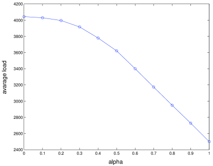
Figure 1: The average load at the vertices is given with respect to the parameter $\alpha$, while keeping the number of vertices fixed (at 500) and of the edge degree (3 per node).

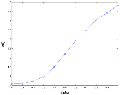
Figure 2: Normalized STD of vertex load $\tilde{\sigma}(l)$ is reported as varying the $\alpha$ parameter, under the same hypothesis of figure 2.

IV Model of Network Data Traffic

We use the family of Erramilli interval maps as the generator for each LRD traffic source, (Erramilli et al., 1994),[12] within the network. The maps are given by $f=f_{(m_{1},m_{2},d)}:I\rightarrow I$, $I=[0,1]$, where:

$$f(x)=\begin{cases}x+(1-d)\left({x/d}\right)^{m_{1}},&x\in[0,d],\cr x-d\left((1-x)/(1-d)\right)^{m_{2}},&x\in(d,1],\end{cases}$$ (2)

where $d\in(0,1)$. The map $f$ is iterated to produce an orbit, or sequence, of real numbers $x_{n}\in[0,1]$ which is then converted into a binary Off-On sequence where the $n$-th value is ’Off’ if $x_{n}\in[0,d]$, and ’On’ if $x_{n}\in(d,1]$. If the map is in the ’On’ state, each iteration of the map represents a packet generated. The parameters $m_{1},m_{2}\in[3/2,2]$ induce map intermittency. When $m_{1}=m_{2}=1.5$ we have short range dependent binary output and this becomes fully long range dependent binary output for ${\rm Max}\{m_{1},m_{2}\}=2.0$.

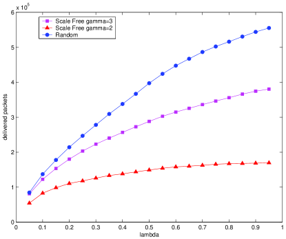
Figure 3: Number of delivered packets versus the generation rate, $\lambda$. Three different networks, random, scale-free with $\gamma=3$, scale-free with $\gamma=2$, have been compared, while keeping a fixed number of vertices (500) and the edge degree (3 per node).

The network involves two types of nodes: hosts and routers. The first are nodes that can generate and receive messages and the second can only store and forward messages. The density of hosts $\rho\in[0,1]$ is the ratio between the number of hosts and the total number of nodes in the network (in this paper we take $\rho=0.16$). Hosts are randomly distributed throughout the network.

A routing algorithm is needed to model the dynamic aspects of the network. Packets are created at hosts and sent through the lattice one step at a time until they reach their destination host.

The routing algorithm operates as follows:

(1) First a host creates a packet following a distribution defined by a chaotic map (LRD), as described above. If a packet is generated it is put at the end of the queue for that host. This is repeated for each host in the lattice.

(2) Packets at the head of each queue are picked up and sent to a neighboring node selected according to the following rules. (a) A neighbor closest to the destination node is selected. (b) If more than one neighbor is at the minimum distance from the destination, the link through which the smallest number of packets have been forwarded is selected. (c) If more than one of these links shares the same minimum number of packets forwarded, then a random selection is made.

This process is repeated for each node in the lattice. The whole procedure of packet generation and movement represents one time step of the simulation.

Figure 4: Delivery times versus the generation rate, $\lambda$. Three different networks, random, scale-free with $\gamma=3$, scale-free with $\gamma=2$, have been compared, while keeping fixed the number of vertices (500) and the edges (3 per node)

V Effects on network performance of varying the underlying topology

We have compared three different topologies: random, scale-free with $\gamma=3$, scale-free with $\gamma=2$ in order to evaluate the effects of the underlying topology on the network performances.

The networks we consider have different degree distributions but are characterized by the same number of available resources, that is by the same number of vertices and edges. For the only case where the resulting network is not fully connected, we have only considered the giant component.

In Fig.3 the number of delivered packets, or throughput, has been plotted as a function of the generation rate, $\lambda$, for the three considered topologies. Scale-free networks show the least effective performances in that the number of delivered packets is lower than for random networks, with Poisson degree distribution. For scale-free networks, those with $\gamma=2$ are still less effective than those with $\gamma=3$. Though our analysis is purely qualitative, we would like to point out that the real Internet has a power-law degree distribution with $\gamma=2.2$ [8].

Notice that the differences among the different considered topologies, increase for higher values of $\lambda$. In particular random networks seem to behave better than other networks under high traffic rates. It is worth noting that this is in strong agreement with results shown in [13].

In Fig.4, the delivery time for packets to reach their destination has been plotted versus the generation rate, $\lambda$. The results are in accordance with those for throughput: the highest delivery time have been achieved for random networks, the lowest for scale-free networks with $\gamma=2$.

The reason for this is that packets that are stored in the routers’ queues without being delivered to their destination, increase the time needed for other packets to reach their destination. Moreover scale-free networks show a vanishing value of the critical load $\lambda$, i.e. the value of $\lambda$ at which a phase-transition occurs [3], with respect to random graphs.

Consequently, although scale-free networks are characterized by a shorter characteristic-path-length [14], they show worst performances in terms of communication. We conjecture this could be explained in terms of load distribution. In fact, as we have already observed, that distribution is characterized by (i) a decreasing mean (ii) an increasing standard deviation, as the networks becomes scale-free (especially scale-free networks with low degree distribution exponents). As a result, since the model is uncontrolled, most packets will go through the bottle-neck vertices, localizing the jamming in some zone of the network, further inducing the onset of congestion.

VI Conclusions

We have shown how topological transitions in a given network from random to scale free affect the load distribution on the network itself. In particular, we characterised such load distribution in terms of the average load and its standard deviation. We observed that as the topological transition takes place, the network performance worsens and the load tends to become more localised (higher standard deviation).

Using a novel LRD traffic generation model, we then characterised the effects of localisation of the load in terms of the typical parameters used to measure performance of traffic on the network; namely the number of delivered packets and the average delivery time.

References

- [1] K.-I. Goh, B. Kahng, and D.Kim, “Universal behavior of load distribution in scale-free networks,” Phys.Rev.Lett., vol. 87, no. 27, 2001.
- [2] L.A.N. Amaral, A. Scala, M.Berth lemy, and H.E.Stanley, “Classes of small-world networks,” Proc.Natl.Acad.Sci.USA, vol. 97, pp. 11149–11152, 2000.
- [3] T. Ohira and R. Sawatari, “Phase transition in a computer network traffic model,” Phys. Rev. E, , no. 58, pp. 193–195, 1998.
- [4] R.V. Sole and S.Valverde, “Information transfer and phase transition in a model of data traffic,” Physica A, vol. 289, no. 595, 2001.
- [5] D.K. Arrowsmith, R.J. Mondrag n, J.M. Pittsy, and M. Woolf, “Phase transitions in packet traffic on regular networks: a comparison of source types and topologies,” 2004.
- [6] P. Erdos and A.Renyi, ,” Publ. Math. Inst. Hung. Acad., vol. 5, no. 17, 1960.
- [7] A.L.Barabasi and R.Albert, “Emergence of scaling in random networks,” Science, vol. 286, pp. 509–512, 1999.
- [8] M.Faloutsos, P.Faloutsos, and C.Faloutsos, “What does internet look like?,” Comput.Commun.Rev., vol. 29, pp. 251–263, 1999.
- [9] S.N.Dorogovstev and J.F.F. Mendes, “Evolution of networks,” Adv. Phys, vol. 1079, no. 51, pp. 1079–1187, 2002.
- [10] L. Freeman, Sociometry, 1977.
- [11] K.-I.Goh, B.Kahng, and D.Kim, “Packet transport and load distribution in scale-free network models,” Physica A, vol. 318, pp. 72–79, 2003.
- [12] A. Erramilli, R.P. Singh, and P. Pruthi, “Chaotic maps as models of packet traffic,” Proc. Int. Teletraffic Conf., 1994, North–Holland (Elsevier).
- [13] A.Arenas, A.Cabrales, A.Diaz-Guilera, R.Guimera, and F.Vega-Redondo, “Search and congestion in complex networks,” cond-mat, vol. 1, no. 0301124, 2003.
- [14] R. Cohen and S.Havlin, “Scale-free networks are ultrasmall,” Phys. Rev.Letters, vol. 90, no. 5, 2003.