Spines of Random Constraint Satisfaction Problems: Definition and Connection with Computational Complexity

Abstract

We study the connection between the order of phase transitions in combinatorial problems and the complexity of decision algorithms for such problems. We rigorously show that, for a class of random constraint satisfaction problems, a limited connection between the two phenomena indeed exists. Specifically, we extend the definition of the spine order parameter of Bollobás et al. [7] to random constraint satisfaction problems, rigorously showing that for such problems a discontinuity of the spine is associated with a $2^{\Omega(n)}$ resolution complexity (and thus a $2^{\Omega(n)}$ complexity of DPLL algorithms) on random instances. The two phenomena have a common underlying cause: the emergence of “large” (linear size) minimally unsatisfiable subformulas of a random formula at the satisfiability phase transition.

We present several further results that add weight to the intuition that random constraint satisfaction problems with a sharp threshold and a continuous spine are “qualitatively similar to random 2-SAT”. Finally, we argue that it is the spine rather than the backbone parameter whose continuity has implications for the decision complexity of combinatorial problems, and we provide experimental evidence that the two parameters can behave in a different manner.

Keywords: constraint satisfaction problems, phase transitions, spine, resolution complexity.

MR Categories: Primary 68Q25, Secondary 82B27.

1 Introduction

The major promise of phase transitions in combinatorial problems has been to shed light on the “practical” algorithmic complexity of combinatorial problems. A possible connection has been highlighted by results of Monasson et al. [1, 2] that are based on experimental evidence and nonrigorous arguments from statistical mechanics. Studying a version of random satisfiability that “interpolates” between 2-SAT and 3-SAT, they suggested that the order of the phase transition, combinatorially expressed by continuity of an order parameter called the backbone, might have implications for the problem’s typical-case complexity. A discontinuous or first-order transition appeared to be symptomatic of exponential complexity, whereas a continuous or second-order transition was correlated with polynomial complexity.

It is understood by now that this connection is limited. For instance, $k$-XOR-SAT is a problem believed, based on arguments from statistical mechanics [3], to have a first-order phase transition. But it is easily solved by a polynomial algorithm, Gaussian elimination. So, if any connection exists between first-order phase transitions and the complexity of a given problem, it cannot involve all polynomial time algorithms for the problem. Fortunately, this does not end all hopes for a connection with computational complexity: descriptive complexity [4] provides a principled way to measure the complexity of problems with respect to more limited classes of algorithms, those expressible in a given framework. Here we focus on the Davis-Putnam-Longman-Loveland (DPLL) class of algorithms [5].

One way to identify the connection between phase transitions and computational complexity is to formalize the underlying intuition connecting the two notions in a purely combinatorial way, devoid of any physics considerations. First-order phase transitions amount to a discontinuity in the (suitably rescaled) size of the backbone. For random $k$-SAT [6], and more specifically for the optimization problem MAX-$k$-SAT, the backbone has a combinatorial interpretation: it is the set of literals that are “frozen”, or assume the same value, in all optimal assignments. Intuitively, a large backbone size has implications for the complexity of finding such assignments: all literals in the backbone require specific values in order to satisfy the formula optimally, but an algorithm assigning variables in an iterative fashion has very few ways to know what those “right” values to assign are. In the case of a first-order phase transition, the backbone of formulas just above the transition contains, with high probability, a fraction of the literals that is bounded away from zero. An algorithm such as DPLL that assigns values to variables iteratively may misassign a backbone variable whose height, in a binary tree characterizing the behavior of the algorithm, is $\Omega(n)$ where $n$ is the number of variables. This would force a backtrack on the tree. Assuming the algorithm cannot significantly “reduce” the size of the explored portion of this tree, a first-order phase transition would then w.h.p. imply a $2^{\Omega(n)}$ lower bound for the running time of DPLL on random instances located slightly above the transition.

There exists, however, a significant flaw in the heuristic argument above: the backbone is defined with respect to optimal assignments for the given formula, meaning assignments that satisfy the largest possible number of clauses (or all of them, in the case where the formula is satisfiable). The argument suggests that a discontinuity in the backbone size will make it difficult for algorithms that assign variables in an iterative manner to find optimal solutions. The complexity of the optimization problem is, however, often different from that of the corresponding decision problem. For instance, that is the case in XOR-SAT, where the decision problem is easy but the optimization problem is hard. As mentioned above, XOR-SAT is presumed to have a first-order phase transition, so it is not clear at all that the continuity or discontinuity of the backbone should be the relevant predictor for the complexity of the decision problem as well.

Fortunately, it turns out that the intuition of the previous argument also holds for a different order parameter, a “weaker” version of the backbone called the spine, introduced in [7] in order to prove that random 2-SAT has a second-order phase transition. Unlike the backbone, the spine is defined in terms of the decision problem, hence it could conceivably have a larger impact on the complexity of these problems. Of course, the same caveat applies as for the backbone: any connection with computational complexity can only involve complexity classes that have weaker expressive power than the class of polynomial time algorithms.

We aim in this paper to provide evidence that for random constraint satisfaction problems it is the behavior of the spine, rather than the backbone, impacts the complexity of the underlying decision problem. To accomplish this:

1. We discuss the proper definitions of the backbone and spine for random constraint satisfaction problems (CSP).

2. We formally establish a simple connection between a discontinuity in the relative size of the spine at the threshold and the resolution complexity of random satisfiability problems. In a nutshell, a necessary and sufficient condition for the existence of a discontinuity is the existence of an $\Omega(n)$ lower bound (w.h.p.) on the size of minimally unsatisfiable subformulas of a random (unsatisfiable) subformula. But standard methods from proof complexity [8] imply that for all problems where we can prove such an $\Omega(n)$ lower bound, there is a $2^{\Omega(n)}$ lower bound on their resolution complexity and hence on the complexity of DPLL algorithms as well [5]. This property arises from the expansion of the underlying formula’s hypergraph, and is independent of the precise definition of the problem at hand. Conversely we show (Theorem 1) that for any generalized satisfiability problem, a second-order phase transition implies, in the region where most formulas are unsatisfiable, an upper bound on resolution complexity that is smaller than any exponential: $O(2^{\epsilon n})$ for every $\epsilon>0$.

3. We give a sufficient condition (Theorem 2) for the existence of a discontinuous jump in the size of the spine. We then show (Theorem 3) that this condition is fulfilled by all problems whose constraints have no implicates of size two or less. Qualitatively, our results suggest that all satisfiability problems with a continuous phase transition in the spine are “2-SAT-like”.

4. Finally, we present experimental results that attempt to clarify whether the backbone and the spine can behave differently at the phase transition. The graph bipartition problem (GBP) is one case where this seems to happen. In contrast, for random 3-coloring (3-COL), the backbone and spine appear to have similar behavior.

A note on the significance of our results: a first-order transition or discontinuity in the size of the spine is weaker than a discontinuity in the size of the backbone. In the last section of the paper we give a numerical demonstration of an example where the backbone and spine behave differently. And unlike for the backbone, we do not have a physical interpretation for the spine. But this is not our intention. The argument connecting the continuity of the backbone order parameter with the complexity of decision problems is problematic, and what we rigorously show is that — with no physical considerations in mind — the intuitive connection holds instead for the spine.

2 Preliminaries

Throughout this paper we assume a general familiarity with the concepts of phase transitions in combinatorial problems [9], random structures [10], and proof complexity [11]. We assume more detailed familiarity with certain fundamental results on sharp thresholds [12, 13, 8], and we make use of some of the methods associated with those results.

Two models arising in the theory of random structures are:

• The constant probability model $\Gamma(n,p)$. A random string of bits $X\in\Gamma(n,p)$ is obtained by independently setting each bit of $X$ to 1 with probability $p$, and the rest to 0.

• The counting model $\Gamma(n,m)$. A random string $X\in\Gamma(n,m)$ is obtained by setting $m$ bits of $X$, chosen uniformly at random, to 1 and the rest to 0.

For the following purposes, let us work within the constant probability model. Consider a property $A$ that is monotonically increasing, in that if $A$ holds for a given string of bits $X$, then changing any of these bits from 0 to 1 preserves property $A$. For any $\epsilon>0$, let $p_{\epsilon}=p_{\epsilon}(n)$ be the canonical probability such that $\mathop{\mathrm{Prob}}_{X\in\Gamma(n,p_{\epsilon}(n))}[X\mbox{ satisfies }A]=\epsilon$, where $p_{\epsilon}$ increases monotonically with $\epsilon$. Sharp thresholds are those for which the function has a “sudden jump” from value 0 to 1:

Definition 1

Property $A$ has a sharp threshold iff for every $0<\epsilon<1/2$, we have $\lim_{n\rightarrow\infty}\frac{p_{1-\epsilon}(n)-p_{\epsilon}(n)}{p_{1/2}(n)}=0$. $A$ has a coarse threshold if for some $\epsilon>0$ it holds that $\lim\inf_{n\rightarrow\infty}\frac{p_{1-\epsilon}(n)-p_{\epsilon}(n)}{p_{1/2}(n)}>0$.

We will use the model of random constraint satisfaction from Molloy [14]:

Definition 2

Let ${\cal D}=\{0,1,\ldots,t-1\}$, $t\geq 2$ be a fixed set. Consider all $2^{t^{k}}-1$ possible nonempty sets of $k$-ary constraint templates (relations) with values taken from ${\cal D}$. Let ${\cal C}$ be such a nonempty set of constraint templates.

A random formula $\phi\in\mathrm{CSP}({\cal C})$ is a set of constraints specified under the counting model by the following procedure:

1. Select, uniformly at random and with replacement, $m$ hyperedges of the complete $k$-uniform hypergraph on $n$ variables.

2. For each hyperedge, choose a random ordering of the variables involved in it. Choose a random constraint template from ${\cal C}$ and apply it to the list of (ordered) variables.

We use the notation $\mathrm{SAT}({\cal C})$ (instead of $\mathrm{CSP}({\cal C})$) when t=2.

For an instance $\Phi\in\mathrm{CSP}({\cal C})$, we denote by $\mathit{Var}(\Phi)$ the set of variables that actually appear in $\Phi$, and by $\mathit{opt}(\Phi)$ the number of constraints left unsatisfied by an optimal assignment for $\Phi$.

Just as in random graphs [10], under fairly liberal conditions one can use the constant probability model instead of the counting model from the previous definition. The interesting range of the parameter $m$ is when the ratio $m/n$ is a constant, $c$, called the constraint density. The original investigation of the order of the phase transition in $k$-SAT used an order parameter called the backbone,

$$B(\Phi)=\{x\in\mathit{Var}(\Phi)\ |\ \exists\ W\in\{x,\overline{x}\}:\mathit{opt}(\Phi\cup W)>\mathit{opt}(\Phi)\},$$ (1)

or more precisely the backbone fraction

$$f_{B}(\Phi)=\frac{|B(\Phi)|}{n}.$$ (2)

Bollobás et al. [7] have investigated the order of the phase transition in $k$-SAT (for $k=2$) under a different order parameter, a “monotonic version” of the backbone called the spine

$$S(\Phi)=\{x\in\mathit{Var}(\Phi)\ |\ \exists\ W\in\{x,\overline{x}\},\Xi\subseteq\Phi:\Xi\in\mathrm{SAT},\Xi\wedge W\in\overline{\mathrm{SAT}}\}.$$ (3)

Here, “$\in\mathrm{SAT}$” means “is satisfiable” and “$\in\overline{\mathrm{SAT}}$” means “is unsatisfiable”.

The corresponding version of Eq. (2) is

$$f_{S}(\Phi)=\frac{|S(\Phi)|}{n}.$$ (4)

They showed that random 2-SAT has a continuous (second-order) phase transition: the size of $f_{S}$ approaches zero w.h.p. (as $n\rightarrow\infty$) for constraint density $c<c_{\mathrm{2-SAT}}=1$, and is continuous at $c=c_{\mathrm{2-SAT}}$. By contrast, nonrigorous arguments from statistical mechanics [6] imply that for 3-SAT the parameter $f_{B}$ jumps discontinuously from zero to a positive value at the transition point $c=c_{\mathrm{3-SAT}}$ (a first-order phase transition).

3 How to define the backbone/spine for random CSP (and beyond)

We would like to extend the concepts of backbone and spine to general constraint satisfaction problems. The extended definitions must preserve as many of the properties of the backbone/spine as possible.

Certain differences between the case of random $k$-SAT and the general case force us to employ an alternative definition of the backbone/spine. The most obvious is that Eq. (3) involves negations of variables, unlike Molloy’s model. Also, these definitions are inadequate for problems whose solution space presents a relabeling symmetry, such as the case of graph coloring where the set of (optimal) colorings is closed under permutations of the colors. Due to this symmetry, no variable can be “frozen” to a fixed value $\lambda$ as in Eq. (1).

We therefore define the backbone/spine of a random instance of $\mathrm{CSP}({\cal C})$ in a slightly different manner. Let $\hat{C}$ be the set of constraints obtained by applying the constraint templates in ${\cal C}$ to all ordered lists of $k$ variables chosen from the set of all $n$ variables.

Definition 3

$$B(\Phi)=\{x\in\mathit{Var}(\Phi)\ |\ \exists\ C\in\hat{C}:x\in C,\mathit{opt}(\Phi\cup C)>\mathit{opt}(\Phi)\},$$

$$S(\Phi)=\{x\in\mathit{Var}(\Phi)\ |\ \exists\ C\in\hat{C},\Xi\subseteq\Phi:x\in C,\Xi\in\mathrm{CSP},\Xi\cup C\in\overline{\mathrm{CSP}}\}.$$

For $k$-CNF formulas whose (original) backbone/spine contains at least three literals, a variable $x$ is in the (new version of the) backbone/spine if and only if either $x$ or $\overline{x}$ were present in the old version. In particular the new definition does not change the order of the phase transition of random $k$-SAT.

Alternatively, in studying 3-colorability (3-COL) of random graphs $G=(V,E)$, Culberson and Gent [16] defined the spine of a colorable graph $G$ to be the set of vertex pairs $(x,y)\in V^{2}$ that get assigned the same color in all colorings of $G$.

Following up on the idea of defining the backbone and spine in terms of constraints rather than variables, and by analogy with the definition in [7], one can extend the definition of $S(G)$ to general graphs by

$$S(G)=\{(x,y)\in V^{2}\ |\ \exists\ H\subseteq G:H\in\mbox{3-COL},H\cup(x,y)\in\overline{\mbox{3-COL}}\}.$$ (5)

We can further extend these definitions to all random constraint satisfaction problems $\mathrm{CSP}({\cal C})$:

Definition 4

$$B_{C}(\Phi)=\{C\in\hat{C}\ |\ \mathit{opt}(\Phi\cup C)>\mathit{opt}(\Phi)\},$$

$$S_{C}(\Phi)=\{C\in\hat{C}\ |\ \exists\ \Xi\subseteq\Phi:\Xi\in\mathrm{CSP},\Xi\cup C\in\overline{\mathrm{CSP}}\}.$$

Similarly, one can define the backbone/spine fraction by

$$f_{B_{C}}(\Phi)=\frac{|B_{C}(\Phi)|}{|\hat{C}|},$$

and

$$f_{S_{C}}(\Phi)=\frac{|S_{C}(\Phi)|}{|\hat{C}|}.$$

We will refer to these concepts as the constraint-based backbone/spine (fractions), as opposed to the previously defined variable-based quantities. The two are clearly related. For instance one can easily show that

$$B(\Phi)=\cup_{C\in B_{C}(\Phi)}\mathit{Var}(C),$$

where $\mathit{Var}(C)$ represents all variables appearing in constraint $C$ alone. It is also clear that $|B_{C}(\Phi)|=O(|B(\Phi)|^{k})$ and similarly for the spine. Since $|\hat{C}|=\Theta(n^{k})$, it follows that the continuity of $f_{B}$ or $f_{S}$ implies the continuity of $f_{B_{C}}$ or $f_{S_{C}}$. However, the converse is not in general true, and so the two backbone/spine fractions do not necessarily behave in the same way.

Given the two types of definitions, which should we choose? The answer depends on the problem, as well as on the issue we wish to address. For instance, in the statistical mechanics analysis of combinatorial problems, the presumably “correct” definition of the backbone emerges from the analysis undertaken in [6] for random $k$-SAT. But since we are interested in a combinatorial definition, with no physics considerations in mind, the only principled way to choose between the two types of order parameters (one based on variables, the other based on constraints) is based on the class of algorithms we are concerned with. In the case of random constraint satisfaction problems and DPLL algorithms, it is variables that get assigned values, so Definition 3 is preferred. On the other hand, constraint-based definitions can make sense for problems that share some characteristics with random 3-COL (i.e., binary constraint satisfaction problems, and problems with built-in symmetries of the solution space). In a later section we will see an example, the case of graph bipartition, where the constraint-based backbone and spine seem to behave differently. (Whether one can come with a natural example of this phenomenon for the variable-based backbone is an interesting open problem.)

4 Spine discontinuity and resolution complexity of random CSP

In this section we will study the continuity of the spine-based order parameter $f_{S}$ for boolean random constraint satisfaction, or satisfiability, problems. The kind of continuous/discontinuous behavior we are looking for is formalized by the following definition (a similar one can be given for the constraint-based versions of the order parameter):

Definition 5

Let ${\cal C}$ be such that $\mathrm{SAT}({\cal C})$ has a sharp threshold. Problem $\mathrm{SAT}({\cal C})$ has a discontinuous spine if there exists $\eta>0$ such that for every sequence $m=m(n)$ we have

$$\lim_{n\rightarrow\infty}\mathop{\mathrm{Prob}}_{m=m(n)}[\Phi\in\mathrm{SAT}]=0\Rightarrow\lim_{n\rightarrow\infty}\mathop{\mathrm{Prob}}_{m=m(n)}[f_{S}(\Phi)\geq\eta]=1.$$ (6)

If, on the other hand, for every $\epsilon>0$ there exists a constant $c=c({\epsilon})$ such that the map $\epsilon\rightarrow c({\epsilon})$ is monotonically increasing and

$$\lim_{n\rightarrow\infty}\mathop{\mathrm{Prob}}_{m=c({\epsilon})n}[\Phi\in\mathrm{SAT}]=0\ \mathrm{and}\ \lim_{n\rightarrow\infty}\mathop{\mathrm{Prob}}_{m=c({\epsilon})n}[f_{S}(\Phi)\geq\epsilon]=0$$ (7)

we say that $\mathrm{SAT}({\cal C})$ has a continuous spine.

We now give a simple observation that will be the basis for identifying discontinuities of the spine:

Proposition 1

Let $\Phi$ be a minimally unsatisfiable formula, and let $x$ be a literal that appears in $\Phi$. Then, by Definition 3, $x\in S(\Phi)$.

Proof.   There exists $C\in\Phi$ such that $x\in C$. But $\Phi\setminus C$ is satisfiable and $(\Phi\setminus C)\cup C$ is not, thus $x\in S(\Phi)$. $\Box$

Corollary 1

$k$-SAT, $k\geq 3$ has a discontinuous spine.

Proof.   To show a discontinuous spine it is sufficient to show that a random unsatisfiable formula contains w.h.p. a minimally unsatisfiable subformula involving a linear number of literals. In the Chvátal-Szemerédi proof [13] that w.h.p. random $k$-SAT has exponential resolution size for $k\geq 3$, the claim is implicitly proved. $\Box$

Definition 6

The width of a resolution proof $P$ of the unsatisfiability of a CNF-formula $F$ is defined to be the maximum number of literals in any clause that appears in the proof $P$.

If $\Phi$ is an instance of $\mathrm{SAT}({\cal C})$, denote by $\mathit{Cl}(\Phi)$ the CNF formula obtained by expressing each constraint of $\Phi$ as a conjunction of clauses (i.e., expressing $\Phi$ in conjunctive form).

The resolution complexity of an instance $\Phi$ of $\mathrm{SAT}({\cal C})$ is defined as the length of the smallest resolution proof of $\mathit{Cl}(\Phi)$.

A simple observation is that a continuous spine has implications for resolution complexity:

Theorem 1

Let ${\cal C}$ be a set of constraint templates such that $\mathrm{SAT}({\cal C})$ has a continuous spine. Then for every constraint density $c>lim_{\epsilon\rightarrow 0}c({\epsilon})$, and every $\epsilon>0$, random formulas of constraint density $c$ have w.h.p. resolution complexity $O(2^{\epsilon n})$.

Proof.

Because of Proposition 1 and the fact that $\mathrm{SAT}({\cal C})$ has a continuous spine, for every $\epsilon>0$, minimally unsatisfiable subformulas of a random formula $\Phi$ with constraint density $c({\epsilon})$ contain w.h.p. at most $\epsilon n$ variables. Consider the backtrack tree of the natural DPLL algorithm that tries to satisfy constraints one at a time on such a minimally unsatisfiable subformula $F$. By the usual correspondence between DPLL refutations and resolution complexity (e.g., [5]) this yields a resolution proof of the unsatisfiability of $\Phi$ having size at most $2^{\epsilon n}$.

Taking $\epsilon$ to be small enough that $c({\epsilon})<c$, and using the fact that resolution complexity of a random formula is a monotonically decreasing function of the constraint density, we get the desired result. $\Box$

Let us observe that we have stated the preceding theorem using condition $c>lim_{\epsilon\rightarrow 0}c({\epsilon})$ since we cannot be sure, even for $k$-SAT, that the phase transition takes place at a constant value of the constraint density $c$. In practice one would of course expect that, for a problem with a continuous spine, there exists a sequence $c({\epsilon})$ as in Definition 5 having the constraint density at the phase transition as its limit.

Definition 7

Denote by $|F|$ the number of constraints that appear in formula $F$. Define

$$c^{*}(F)=\max\left\{\frac{|H|}{|\mathit{Var}(H)|}:\emptyset\neq H\subseteq F\right\}.$$

The next result gives a sufficient condition for a generalized satisfiability problem to have a discontinuous spine. Interestingly, it is one condition studied in [14].

Theorem 2

Let ${\cal C}$ be such that $\mathrm{SAT}({\cal C})$ has a sharp threshold. If there exists $\epsilon>0$ such that for every minimally unsatisfiable formula $F$ it holds that $c^{*}(F)>\frac{1+\epsilon}{k-1}$, then $\mathrm{SAT}({\cal C})$ has a discontinuous spine.

Proof.   The proof is similary to that of Corollary 1: we will show that w.h.p. a random formula contains a minimally unsatisfiable subformula containing a linear number of variables, and apply Proposition 1.

To accomplish that, we first recall the following concept from [13]:

Definition 8

Let $x,y>0$. A $k$-uniform hypergraph with $n$ vertices is ($x$,$y$)-sparse if every set of $s\leq xn$ vertices contains at most $ys$ edges.

We also recall Lemma 1 from the same paper.

Lemma 1

Let $k,c>0$ and $y>1/(k-1)$. Then w.h.p. the random $k$-uniform hypergraph with $n$ vertices and $cn$ edges is $(x,y)$-sparse, where

$$x=\left(\frac{1}{2e}\left(\frac{y}{ce}\right)^{y}\right)^{\frac{1}{y(k-1)-1}}.$$ (8)

Let $y=\frac{1+\epsilon}{k-1}$. Directly applying Lemma 1, w.h.p. a random $k$-uniform hypergraph with $cn$ edges is $(x_{0},y)$ sparse, for $x_{0}=(\frac{1}{2e}(\frac{y}{ce})^{y})^{\frac{1}{\epsilon}}$. The critical observation is then that the existence of a minimally unsatisfiable formula with $xn$ variables and with $c^{*}(F)>\frac{1+\epsilon}{k-1}$ implies that the $k$-uniform hypergraph associated with the given formula is not $(x,y)$-sparse. It follows that any formula with fewer than $x_{0}n/k$ constraints (and thus fewer than $x_{0}n$ variables) is satisfiable. Therefore, any minimally unsatisfiable subformula of random formula $\Phi$ has more than $x_{0}n/k$ constraints.

To show that such formulas have many variables, we again employ the expansion of the formula hypergraph given by Lemma 1, and infer that all subformulas of size less than $xn$ of $\Phi$ (in particular those that are also subformulas of a minimally unsatisfiable subformula of $\Phi$) have a linear number of variables. $\Box$

One can give an explicitly defined class of satisfiability problems for which the previous result applies:

Theorem 3

Let $k\geq 2$ and let ${\cal C}$ be such that $\mathrm{SAT}({\cal C})$ has a sharp threshold. If no clause template $C\in{\cal C}$ has (when expressed as a CNF-formula) an implicate of length 2 or 1 then

1. For every minimally unsatisfiable formula $F$, $c^{*}(F)\geq\frac{2}{2k-3}$. Therefore $\mathrm{SAT}({\cal C})$ satisfies the conditions of the previous theorem, i.e., it has a discontinuous spine.

2. Moreover, there exists a constant $\eta>0$ such that w.h.p. random instances of $\mathrm{SAT}({\cal C})$ have $\Omega(2^{\eta n})$ resolution complexity.

The condition in the theorem is violated, as expected, by random 2-SAT. It is also violated by the random version of the NP-complete problem 1-in-$k$-SAT. This can be seen as follows. The problem can be represented as $\mathrm{CSP}({\cal C})$, for ${\cal C}$ a set of $2^{k}$ constraints corresponding to all ways to negate some of the variables, and has a rigorously determined “2-SAT-like” location of the transition point [19]. However, the formula

$$C(x_{1},x_{2},\ldots,x_{k-1},x_{k})\wedge C(\overline{x_{k}},x_{k+1},\ldots,x_{2k-2},x_{1})$$

$$\wedge C(\overline{x_{1}},x_{2k-1},\ldots,x_{3k-3},\overline{x_{k}})\wedge C(x_{k},x_{3k-2},\ldots,x_{4k-4},\overline{x_{1}}),$$

where $C$ is the constraint “1-in-$k$”, is minimally unsatisfiable but has clause/variable ratio $1/(k-1)$ and implicates $\overline{x_{1}}\vee\overline{x_{k}}$ and $x_{1}\vee x_{k}$.

Proof.

1. For any real $r\geq 1$, formula $F$ and set of clauses $G\subseteq F$, define the $r$-deficiency of $G$, $\delta_{r}(G)=r|G|-2|\mathit{Var}(G)|$. Also define

   $$\delta^{*}_{r}(F)=\max\{\delta_{r}(G):\emptyset\neq G\subseteq F\}$$ (9)

   Definition 9

   Let $F$ be a formula, and let $C_{1},C_{2},\ldots,C_{i},\ldots,C_{m}$ be a listing of the constraints in $F$.

2. A variable $v$ is private for constraint $C_{i}$ if $v$ appears in $C_{i}$ but in no other constraint.

3. Variable $v$ is free in $C_{i}$ if $v$ appears in $C_{i}$ but in no $C_{j}$, $j<i$. Otherwise we say that $v$ is bound in $C_{i}$.

   We claim that for any minimally unsatisfiable $F$, $\delta^{*}_{2k-3}(F)\geq 0$. Indeed, assume this was not true. Then there exists such $F$ such that:

   $$\delta_{2k-3}(G)\leq-1\mbox{ for all }\emptyset\neq G\subseteq F.$$ (10)

   Lemma 2

   Let $F$ be a formula for which condition 10 holds. Then there exists an ordering $C_{1},\ldots,C_{|F|}$ of constraints in $F$ such that each constraint $C_{i}$ contains at least $k-2$ variables that are free in $C_{i}$.

   Proof.   Denote by $v_{i}$ the number of variables that appear in exactly $i$ constraints of $F$. We have $\sum_{i\geq 1}iv_{i}=k|F|$, therefore $2|\mathit{Var}(F)|-v_{1}\leq k|F|$. This can be rewritten as $v_{1}\geq 2|\mathit{Var}(F)|-k|F|>|F|(2k-3-k)=(k-3)|F|$, where we use Eq. (10). Therefore there exists at least one constraint $C$ in $F$ with at least $k-2$ variables that are private in $F$, hence necessarily free in $F$. We set $C_{|F|}=C$ and apply this argument recursively to $F\setminus C$. $\Box$
   

   Let us show now that $F$ cannot be minimally unsatisfiable. Construct a satisfying assignment for $F$ incrementally, so that the partial assignment constructed up to stage $j$ will satisfy constraints $C_{1},\ldots,C_{j}$.

   Indeed, suppose we have constructed a partial assignment that satisfies $C_{1},\ldots,C_{j-1}$, and consider now constraint $C_{j}$. At most two of the variables in $C_{j}$ are bound in $C_{j}$. Since $C_{j}$ has no implicates of length two or less, no matter what the assignment to these two variables might have been in the previous stages, one can set the variables that are free in $C_{j}$ in a way that satisfies this clause. Iteratively performing this construction yields a satisfying assignment for $F$, in contradiction with our assumption that $F$ was minimally unsatisfiable.

   Therefore $\delta^{*}_{2k-3}(F)\geq 0$, a statement equivalent to our conclusion.

4. To prove the resolution complexity lower bound we use the size-width connection for resolution complexity obtained in [8]: it is sufficient to prove that there exists $\eta>0$ such that w.h.p. random instances of $\mathrm{SAT}({\cal C})$ having constraint density $c$ have resolution width at least $\eta n$.

   To accomplish this, we use the same strategy as in [8]: define for a unsatisfiable formula $\Phi$ a measure $\mu:Clauses\rightarrow{\bf N}$ (where $Clauses$ is the set of all possible disjunctions of literals from $\mathit{Var}(\Phi)$, including the contradictory clause $\Box$) such that

   1. for every clause $C$ that appears in $\mathit{Cl}(\Phi)$, $\mu(C)\leq 1$,

   2. w.h.p. $\mu(\Box)$ is “large”.

   3. Infer that in any refutation there exists a clause $C$ with “medium” $\mu(C)$, and

   4. prove that if $\mu(C)$ is “medium” than the width of $C$ is “large”.

   As in [8], define

   $$\mu(C)=\min\{|\Xi|:\Xi\subseteq\Phi,\Xi\models C\},$$

   where $\models$ is the logical entailment relation. In particular $\mu(\Box)$ is the size of the smallest unsatisfiable subformula of $\Phi$. $\mu$ is subadditive, that is, for every clauses $C_{1}$ and $C_{2}$ that share a variable $x$ appearing with opposite signs in the two clauses,

   $$\mu(res_{x}(C_{1},C_{2}))\leq\mu(C_{1})+\mu(C_{2}).$$

   where $res_{x}(C_{1},C_{2})$ denotes the clause obtained by applying resolution to clauses $C_{1}$, $C_{2}$ with respect to variable $x$. It is clear that condition a) is satisfied. As to b), the following is true:

   Lemma 3

   There exists $\eta_{1}>0$ such that for any $c>0$, w.h.p. $\mu(\Box)\geq\eta_{1}n$, where $\Phi$ is a random instance of $\mathrm{SAT}({\cal C})$ having constraint density $c$.

   Proof.   In the proof of Theorem 2 we have shown that there exists $\eta_{0}>0$ such that w.h.p. any unsatisfiable subformula of a given formula has at least $\eta_{0}n$ constraints. Therefore any formula $F$ made up of clauses from the CNF-representation of constraints in $\Phi$, and which has fewer than $\eta_{0}n$ clauses is satisfiable (since it is less tight than the conjunction of those constraints).

   The claim now follows by taking $\eta_{1}=\eta_{0}$. $\Box$
   

   The only (slightly) nontrivial step of the proof, which critically uses the fact that constraints in ${\cal C}$ do not have implicates of length one or two, is to prove that clause implicates of subformulas of “medium” size have “many” variables.

   Lemma 4

   There exists $d>0$ and $\eta_{2}>0$ such that w.h.p. (when $\Phi$ is a random instance of $\mathrm{SAT}({\cal C})$ having constraint density $c$) every clause $C$ present in a refutation of $\mathit{Cl}(\Phi)$ that satisfies $\frac{dn}{2}<\mu(C)\leq dn$ also satisfies $|C|\geq\eta_{2}n$.

   Proof.

   Given a clause $C$, let $\Xi$ be a subformula of $\Phi$, having minimal size, such that $\Xi\models C$. We claim:

   Lemma 5

   For every constraint $P$ of $\Xi$ that contains $k-2$ private variables, at least one of these variables appears in $C$.

   Proof.   Suppose there exists a constraint $D$ of $\Xi$ with at least $k-2$ private variables such that none of its private variables appears in $C$. Because of the minimality of $\Xi$ there exists an assignment $F$ that satisfies $\Xi\setminus\{D\}$ but does not satisfy $D$ or $C$. Since $D$ has no implicates of size two, there exists an assignment $G$, that differs from $F$ only on the private variables of $D$, that satisfies $\Xi$. But since $C$ does not contain any of the private variables of $D$, $F$ coincides with $G$ on variables in $C$. The conclusion is that $G$ does not satisfy $C$, contradicting the fact that $\Xi\models C$. $\Box$
   

   Now define $x(\cdot,\cdot)$ to be the function from Eq. (8) that describes the dependence of $x$ on $y$ and $c$. For a constant $\epsilon>0$ to be determined later, define

   $$d=min(inf\{x(2/(2k-3+\epsilon),c)|c\geq c_{\mathrm{SAT}({\cal C})}\},\eta_{1}).$$

   Since $\mathrm{SAT}({\cal C})$ has a sharp threshold, the first term of the minimum expression is, like $\eta_{1}$, strictly greater than zero. Therefore, $d>0$.

   Lemma 6

   There exists constant $\eta_{2}>0$ such that w.h.p., when $\Phi$ is a random instance of $\mathrm{SAT}({\cal C})$ having constraint density $c$ and $W\subseteq\Phi$ is a formula with at most $dn$ constraints, $W$ contains at least $\eta_{2}n$ constraints each of which has at least $k-2$ private variables.

   Proof.

   To prove Lemma 6 we first need:

   Lemma 7

   Let $\epsilon>0$ be a constant. If $F$ is a formula with $c^{*}(F)\leq\frac{2}{2k-3+\epsilon}$ then for every subformula $G$ of $F$, at least $(\epsilon/3)|G|$ constraints of $G$ have at least $k-2$ private variables.

   Proof.   Indeed, since $c^{*}(G)\leq\frac{2}{2k-3+\epsilon}$, by an argument similar to the one used in the proof of Lemma 2, $v_{1}(G)\geq(k-3+\epsilon)|G|$. Since constraints in $G$ have arity $k$, at least $(\epsilon/3)|G|$ have more than $k-3$ (i.e., at least $k-2$) private variables. $\Box$
   

   Returning to the proof of Lemma 6, choose $y=\frac{2}{2k-3+\epsilon}$ in Lemma 1 for $\epsilon>0$ a small enough constant. Because of the definition of $d$, when $\Phi$ is a random instance of $\mathrm{SAT}({\cal C})$ having constraint density $c$, w.h.p. formula $\Phi$ is $(d,y)$ sparse. Since $|W|\leq dn$, this easily implies the fact that

   $$c^{*}(W)\leq\frac{2}{2k-3+\epsilon}.$$

   Lemma 6 follows by applying Lemma 7 to formula $W$ with $\eta_{2}=\epsilon/3$. Applying this result and Lemma 5 to formula $\Xi$ also concludes the proof of Lemma 4.

   $\Box$
   

   The proof of item 2. of Theorem 3 now follows: since for any clause $K$ in $\mathit{Cl}(\Phi)$ we have $\mu(K)=1$, since $\mu(\Box)>\eta_{1}n$ and since $0<d\leq\eta_{1}$, there indeed exists a clause $C$ such that

   $$\mu(C)\in[dn/2,dn].$$ (11)

   Indeed, let $C^{\prime}$ be a clause in the resolution refutation of $\Phi$ minimal with the property that $\mu(C^{\prime})>dn$. Then at least one clause $C$ of the two involved in deriving $C^{\prime}$ satisfies Eq. (11). Applying Lemma 4 we infer that the width of $C$ is at least $\eta_{2}n$. Using the size-width connection from[8] completes the proof of item 2. of Theorem 3.

     

4.1 Threshold location and discontinuous spines

Molloy [14] has studied threshold properties of random constraint satisfaction problems, describing a technical property of the constraint set (called very well-behavedness) that is necessary for the existence of a sharp threshold. In [27] we have shown that Molloy’s well-behavedness condition is actually necessary and sufficient for boolean constraints (this has been independently proved by Creignou and Daudé [28]). Thus we have completely characterized sets $C$ for which $\mathrm{SAT}({\cal C})$ has a sharp threshold.

The well-behavedness condition has implication for the clause/variable ratio of minimally unsatisfiable formulas: it has to be larger than $1/(k-1)$. Furthermore, Molloy has shown that if the density of minimally unsatisfiable formulas is bounded away from $1/(k-1)$ (i.e., it satisfies the conditions of Theorem 2) then the location of the transition is strictly larger than $\frac{1}{k(k-1)}$.

We have seen that the same density condition is sufficient to guarantee the discontinuity of the spine and exponential resolution complexity. A natural question therefore arises: is it possible to relate the continuity (or discontinuity) of the spine to the location of the phase transition ?

At first this does not seem to be possible: we have already encountered two problems that fail to satisfy the sufficient condition for a discontinuous spine, random 2-SAT, for which the transition has been proven to be of second order [7], and random 1-in-$k$-SAT, for which a similar result holds [19]. Both have a threshold location strictly higher than Molloy’s lower bound of $\frac{1}{k(k-1)}$. However, the most natural specification of the random model for the two problems involves applying constraints on both variables and their negations. For both problems the actual location of the threshold is twice the value given by Theorem 3 in [14], at clause/variable ratio $\frac{2}{k(k-1)}$. This suggests that the following tempting intuitive picture might be accurate, at least in a more restricted setting:

1. Problems with a continuous spine are “2-SAT-like”, and have a phase transition at constraint density $c^{\mathit{cont}}_{k}=\frac{2}{k(k-1)}$.

2. Problems with a discontinuous spine have a phase transition located at constraint density $c>c^{\mathit{cont}}_{k}$.

To obtain results that partly support the intuition above, we have to modify the random model from Definition 2 to allow negated variables.

Definition 10

Let ${\cal C}$ be a set of constraint templates. The closure of ${\cal C}$, denoted $\overline{\cal C}$ is the set of constraints

$$\overline{\cal C}=\{C(x_{1}^{\epsilon_{1}},\ldots,x_{k}^{\epsilon_{k}})\mbox{ }|\mbox{ }C\in{\cal C}\mbox{ and }\epsilon_{1},\ldots,\epsilon_{k}\in\{\pm 1\}\},$$ (12)

where for a variable $x_{i}$ we define $x_{i}^{1}:=x_{i}$, $x_{i}^{-1}:=\overline{x_{i}}$.

Set ${\cal C}$ is good if $|\overline{\cal C}|=|{\cal C}|2^{k}$, that is all elements on the right hand side of Eq. (12) are distinct.

Definition 11

Let ${\cal C}$ be a good set of constraint templates. Denote by $\mathrm{SAT}^{\mathrm{(neg)}}({\cal C})$ the version of $\mathrm{SAT}({\cal C})$ that generates a random formula by the following process:

1. Select, uniformly at random and with replacement, $m$ hyperedges of the complete $k$-uniform hypergraph on $n$ variables.

2. For each hyperedge $e$, choose a random ordering $o_{e}$ of the variables involved in it.

3. Independently with probability 1/2 negate each variable appearing in $o_{e}$.

4. Choose a random constraint template from ${\cal C}$ and apply it to the ordered list of literals in $o_{e}$.

It is easy to see that problems such as $k$-SAT and 1-in-$k$-SAT can be expressed using the framework of Definition 11. The following result shows that the intuition connecting the discontinuity of the spine, resolution complexity and the location of the phase transition does indeed have merit: a strenghtening of the condition guaranteeing the existence of a discontinuous spine and exponential resolution complexity also implies that the satisfiability threshold is located at a value higher than $c^{\mathit{cont}}_{k}$:

Theorem 4

Let ${\cal C}$ be a good set such that

1. $\mathrm{SAT}^{\mathrm{(neg)}}({\cal C})$ has a sharp threshold (the result in [27] can be easily adapted to completely characterize such sets ${\cal C}$).

2. There exists $\epsilon>0$ such that, for every minimally unsatisfiable formula $F$ whose constraints are drawn from template set ${\cal C}$, the ratio of the number of constraints in $F$ to the number of distinct literals (variables and negated variables) appearing in $F$ is at least $\frac{1+\epsilon}{k-1}$.

Then

1. There is a constant $\delta>0$ such that random instances of $\mathrm{SAT}^{\mathrm{(neg)}}({\cal C})$ with $m=cn$, where $c\leq\frac{2}{k(k-1)}(1+\delta)$, are satisfiable with probability $1-o(1)$.

2. Problem $\mathrm{SAT}^{\mathrm{(neg)}}({\cal C})$ has a discontinuous spine and exponential resolution complexity.

Proof.

1. Since $\mathrm{SAT}^{\mathrm{(neg)}}({\cal C})$ has a sharp threshold, it is sufficient to show that there exists a fixed constant $\eta>0$ such that the probability that a random formula is satisfiable is at least $\eta$.

   Suppose $m=cn$ with $c=\frac{2}{k(k-1)}(1+\delta)$, with $\delta>0$ small enough. Define random model $\mathrm{SAT}^{\mathrm{(neg)}}_{2}({\cal C})$ that is a variant of $\mathrm{SAT}^{\mathrm{(neg)}}({\cal C})$ as follows:

   1. Choose a random $k$-uniform hypergraph $H$ with $m$ edges on the vertex set (of cardinality $2n$) consisting of variables and negated variables.

   2. For every edge $e\in H$ create a random permutation $o_{e}$ of its elements.

   3. Apply a random constraint template in ${\cal C}$ to variables in the ordered list $o_{e}$.

   This model differs from the random model $\mathrm{SAT}^{\mathrm{(neg)}}({\cal C})$ in that it allows for constraints that include a $k$-tuple of literals involving two opposite literals.

   Define $W$ to be the event that formula $\Phi$ contains some clause involving two opposite literals. It is easy to see that the expected number of such clauses in a random formula $\Phi$ is constant. Therefore, with positive probability $\lambda>0$ in a random formula generated according to $\mathrm{SAT}^{\mathrm{(neg)}}_{2}({\cal C})$, the bad event $W$ will not happen.

   Let $Z$ denote the event that a random formula with $m=cn$ clauses generated according to the random model $\mathrm{SAT}^{\mathrm{(neg)}}_{2}({\cal C})$ is satisfiable.

   Then the probability that a random formula in $\mathrm{SAT}^{\mathrm{(neg)}}({\cal C})$ is satisfiable is equal to $Pr[Z|\overline{W}]$. To show that this is bounded away from zero it is enough to prove that $Pr[Z]=1-o(1)$.

   The $k$-uniform hypergraph on the $2n$ nodes (variables and their negations) corresponding to choosing a random instance of $\mathrm{SAT}^{\mathrm{(neg)}}_{2}({\cal C})$ is a random $k$-uniform hypergraph. Thus we want to show that a formula generated by first choosing such a random $k$-uniform hypergraph $H$, and then applying a random constraint template from ${\cal C}$ on the given literals is w.h.p. satisfiable.

   The proof of this is entirely similar to a step in the proof of Molloy’s Theorem 3 in [14], and amounts to showing that w.h.p. the hypergraph $H$ does not contain any hypergraph of high density, corresponding to the fact that minimally unsatisfiable subformulas have clause/variable density at least $\frac{1}{k-1}(1+\epsilon)$. Rather than repeating an argument that is presented in detail in that paper, we refer the reader to [14].

2. Since ${\cal C}$ is good, one can simply apply Theorem 2 to $\mathrm{SAT}(\overline{{\cal C}})$, which is equivalent to problem $\mathrm{SAT}^{\mathrm{(neg)}}({\cal C})$.

$\Box$

5 Beyond random satisfiability: comparing the behavior of the backbone and spine

In this section we investigate empirically the continuity of the backbone for two graph problems, random three coloring (3-COL) and the graph bipartition problem (GBP). Both can be phrased as decision or as optimization problems, in the same manner as $k$-SAT and MAX-$k$-SAT.

We consider a large number of instances of random graphs, of sizes up to $n=1024$ and over a range of mean degree values near the threshold. For each instance we determine the backbone fraction $f$.

Culberson and Gent [16] have shown experimentally that the 3-COL spine fraction $f_{S_{C}}$, as defined in Definition 4, exhibits a discontinuous transition. To be consistent with this study, we use the backbone fraction $f_{B_{C}}$ from the same definition. We employ a rapid heuristic called extremal optimization [20]. Although an incomplete procedure, numerical studies [21] as well as testbed comparisons with an exact algorithm  [23], have shown that extremal optimization yields an excellent approximation of $f_{B_{C}}$ around the critical region (see [20] for further discussions, that, we believe, convincingly support this assertion). Fig. 1 shows $f_{B_{C}}$ as a function of mean degree.

Culberson and Gent have speculated that at the 3-COL threshold, although their spine is discontinuous, the backbone might be continuous. The results in Fig. 1a suggest otherwise. For 3-COL, $f_{B_{C}}$ does not appear to vanish above the threshold, indicating a discontinuous large $n$ backbone [21].

We next study the graph bipartion problem (GBP):

Definition 12

GBP is the following decision problem. Given a (not necessarily connected) graph $G$ with $n$ vertices, $n$ being an even number, determine whether it can be partitioned into two edge-disjoint sets having $n/2$ vertices each.

This problem cannot, strictly speaking, be cast in the setup of random constraint satisfaction problems from Definition 2, since not every partition of vertices of $G$ is allowed. It can be cast to a satisfiability problem (with variables associated to nodes, values associated to each partition and constraint “$x=y$” associated to the edge between the corresponding vertices) but we must add the additional requirement that all satisfying assignments contain an equal number of ones and zeros. Thus the complexity-theoretic observations of Section 4 do not automatically apply to it. We can, however, give a “DPLL-like” class of algorithms for GBP, so the the hope of obtaining results similar to the previous ones is not so far-fetched.

Let us investigate the continuity of the backbone/spine under the model in Definition 4. It is easy to see that the constraint-based spine $S_{C}(G)$ of a GBP instance $G$ contains all edges belonging to a connected component of size larger than $n/2$. Since the GBP threshold takes place where the giant component becomes larger than $n/2$, $f_{S_{C}}$ is discontinuous there. On the other hand, the backbone fraction $f_{B_{C}}$ (Fig. 1b) appears to remain continuous, vanishing at large $n$ on both sides of the threshold.

We have noted earlier that the discontinuity of $f_{B_{C}}$ is a stronger property than the discontinuity of $f_{B}$. Thus for 3-COL it follows that the variable-based backbone is discontinuous as well. By contrast, it is not clear for GBP whether the variable-based backbone is continuous: our preliminary experimental evidence is as yet inconclusive.

The results in Fig. 1b suggest that the spine and the backbone can behave differently at the threshold, though they do not yet address the question of whether the spine’s discontinuity really has computational implications for the decision problem’s complexity. After all, unlike 3-COL, GBP can easily be solved in polynomial time by dynamic programming. This situation is similar to that of XOR-SAT, where a polynomial algorithm exists but the complexity of resolution proofs/DPLL algorithms is exponential. The class of “DPLL-like” algorithms that can solve GBP can no longer be simulated in a straightforward manner by resolution proofs, however it can be simulated using proof systems $Res(k)$ that are extensions of resolution [24]. Some of the hardness results for resolution extend to these more powerful proof systems, and in [26] we investigate the extent to which our present results apply to this class of proof systems. These preliminary results imply that, indeed, the discontinuity of the spine does have computational implications for GBP.

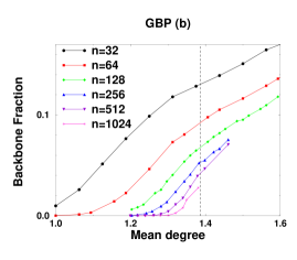
(a) 3-COL [21] (b) GBP.

Figure 1: Plot of the estimated constraint-based backbone fraction $f_{B_{C}}$ on random graphs, as a function of mean degree $c$. For 3-COL, the systematic error based on benchmark comparisons with random graphs is negligible compared to the statistical error bars; for GBP, $f_{B_{C}}$ is found by exact enumeration. The thresholds $c\approx 4.70$ for 3-COL and $c=2\ln 2$ for GBP are shown by dashed lines.

6 Discussion

We have shown that the existence of a discontinuous spine in a random satisfiability problem is often correlated with a $2^{\Omega(n)}$ peak in the complexity of resolution/DPLL algorithms at the transition point. The underlying reason is that the two phenomena (the jump in the order parameter and the resolution complexity lower bound) have common causes.

The example of random $k$-XOR-SAT shows that a general connection between a first-order phase transition and the complexity of the underlying decision problems is hopeless: Ricci-Tersenghi et al. [3] have presented a non-rigorous argument using the replica method that shows that this problem has a first-order phase transition, and the following weaker result is a direct consequence of Theorem 3:

Proposition 2

Random $k$-XOR-SAT, $k\geq 3$, has a discontinuous spine.

However, our results, as well as work in progress mentioned above, suggest that the continuity/discontinuity of the spine is a predictor for the complexity of the restricted classes of decision algorithms that can be simulated by “resolution-like” proof systems. Furthermore, experimental evidence in the previous section suggests that the backbone and the spine do not always behave similarly. Our analysis indicates that the spine, rather than the backbone, is the order parameter to consider in studying the complexity of combinatorial problems.

7 Acknowledgments

This work has been supported by the U.S. Department of Energy under contract W-705-ENG-36, through the LANL LDRD program, and by grant 0312510 from the Division of Materials Research at the National Science Foundation.

References

- [1] R. Monasson, R. Zecchina, S. Kirkpatrick, B. Selman, and L. Troyansky. Determining computational complexity from characteristic phase transitions. Nature, 400(8):133–137, 1999.
- [2] R. Monasson, R. Zecchina, S. Kirkpatrick, B. Selman, and L. Troyansky. -SAT: Relation of typical-case complexity to the nature of the phase transition. Random Structures and Algorithms, 15(3–4):414–435, 1999.
- [3] F. Ricci-Tersenghi, M. Weight, and R. Zecchina. Simplest random -satisfiability problem. Physical Reviews E, 63:026702, 2001.
- [4] N. Immerman. Descriptive Complexity. Springer Graduate Texts in Computer Science, 1999.
- [5] P. Beame, R. Karp, T. Pitassi, and M. Saks. The efficiency of resolution and Davis-Putnam procedures. SIAM Journal of Computing, 31(4):1048–1075, 2002.
- [6] R. Monasson and R. Zecchina. Statistical mechanics of the random -SAT model. Physical Review E, 56:1357, 1997.
- [7] B. Bollobás, C. Borgs, J.T. Chayes, J. H. Kim, and D. B. Wilson. The scaling window of the 2-SAT transition. Technical report, Los Alamos e-print server, http://xxx.lanl.gov/ps/math.CO/9909031, 1999.
- [8] E. Ben-Sasson and A. Wigderson. Short Proofs are Narrow:Resolution made Simple. Journal of the ACM, 48(2), 2001.
- [9] O. Martin, R. Monasson, and R. Zecchina. Statistical mechanics methods and phase transitions in combinatorial optimization problems. Theoretical Computer Science, 265(1-2):3–67, 2001.
- [10] B. Bollobás. Random Graphs. Academic Press, 1985.
- [11] P. Beame and T. Pitassi. Propositional proof complexity: Past present and future. In Current Trends in Theoretical Computer Science, pages 42–70. 2001.
- [12] E. Friedgut. Necessary and sufficient conditions for sharp thresholds of graph properties, and the k-SAT problem. with an appendix by J. Bourgain. Journal of the A.M.S., 12:1017–1054, 1999.
- [13] V. Chvátal and E. Szemerédi. Many hard examples for resolution. Journal of the ACM, 35(4):759–768, 1988.
- [14] M. Molloy. Models for random constraint satisfaction problems. In Proceedings of the 32nd ACM Symposium on Theory of Computing, 2002.
- [15] D. Achlioptas and E. Friedgut. A sharp threshold for -colorability. Random Structures and Algorithms, 14(1):63–70, 1999.
- [16] J. Culberson and I. Gent. Frozen development in Graph Coloring. Theoretical Computer Science, 265(1-2):227–264, 2001.
- [17] D. Mitchell. Resolution complexity of Random Constraints. In Eigth International Conference on Principles and Practice of Constraint Programming, 2002.
- [18] M. Molloy and M. Salavatipour. The resolution complexity of random constraint satisfaction problems. (to appear in FOCS’2003).
- [19] D. Achlioptas, A. Chtcherba, G. Istrate, and C. Moore. The phase transition in random 1-in-k SAT and NAE 3SAT. In Proceedings of the 13th ACM-SIAM Symposium on Discrete Algorithms, 2001. Journal version in preparation.
- [20] S. Boettcher and A. Percus. Nature’s way of optimizing. Artificial Intelligence, 119:275–286, 2000.
- [21] S. Boettcher and A.G. Percus. Extremal Optimization at the Phase Transition of the 3-Coloring Problem. Physical Review E, vol. 69,066703, 2004.
- [22] S. Boettcher. Extremal optimization of graph partition at the percolation threshold. J. Phys. A: Math. Gen., 32:5201–5211, 1999.
- [23] M.A. Trick. color.c graph coloring code. Available at http://mat.gsia.cmu.edu/COLOR/solvers/trick.c.
- [24] J. Krajicek. On the weak pigeonhole principle. Fundamenta Matematicae, 170(1–3):123–140, 2001.
- [25] G. Istrate. Phase transitions and all that. Preprint CS.CC/0211012, ACM Computer Repository at arXiv.org.
- [26] G. Istrate. Descriptive complexity and first-order phase transitions. (in progress).
- [27] G. Istrate. Threshold Properties of Random Constraint Satisfaction Problems. Accepted to a special volume of Discrete Applied Mathematics on Typical-case complexity and phase transitions.
- [28] N. Creignou and H. Daudé. Combinatorial sharpness criterion and phase transition classification for random CSPs . Information and Computation, vol. 190, no.2 (2004), pp. 220-238.