Geometric Models of Rolling-Shutter Cameras

Abstract

Cameras with rolling shutters are becoming more common as low-power, low-cost CMOS sensors are being used more frequently in cameras. The rolling shutter means that not all scanlines are exposed over the same time interval. The effects of a rolling shutter are noticeable when either the camera or objects in the scene are moving and can lead to systematic biases in projection estimation. We develop a general projection equation for a rolling shutter camera and show how it is affected by different types of camera motion. In the case of fronto-parallel motion, we show how that camera can be modeled as an X-slit camera. We also develop approximate projection equations for a non-zero angular velocity about the optical axis and approximate the projection equation for a constant velocity screw motion. We demonstrate how the rolling shutter effects the projective geometry of the camera and in turn the structure-from-motion.

1 Introduction

The motivation for this paper is the use of inexpensive camera sensors for robotics. Maintaining accuracy in this low-cost realm is difficult to do, especially when sacrifices in sensor design are made in order to reduce cost or power consumption. For example, as of 2004, many of the CMOS chips manufactured by OEMs and integrated into off-the-shelf cameras do not have a global shutter. Unlike CCD chips with interline transfer, the individual pixels in a CMOS camera chip typically cannot hold and store intensities, forcing a so-called rolling shutter whereby each scanline is exposed, read out, and in the case of most Firewire cameras, is immediately transmitted to the host computer. Furthermore, for cameras connected via a Firewire bus, the digital camera specification [1] requires that cameras distribute data over a constant number of packets regardless of the framerate. Thus, if the camera has no on-board buffer, the overall exposure for a single frame is inversely proportional to the framerate.

However, most structure-from-motion algorithms (see e.g. [4, 6]) make the assumption that the exposure of frames is instantaneous, and that every scanline is exposed at the same time. If either the camera is moving or the scene is not static then the rolling shutter will induce geometric distortions when compared with a camera equipped with a global shutter. Consider, for example, Figure 1 which shows the distortion present in the image of a fronto-parallel checkerboard when a rolling-shutter equipped camera is rotating about the optical axis.

The fact that every scanline is exposed at a different time will lead to systematic biases in motion and structure estimates.Thus, in considering the design of a robotic platform,which often by necessity is in motion (for example a helicopter) one needs to balance accuracy, cost and power consumption. The goal of this paper is to obviate this trade-off. By modeling the rolling-shutter distortion we mitigate the reduction in accuracy and present a framework for analyzing structure-from-motion problems in rolling-shutter cameras

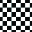
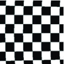
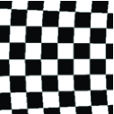
Figure 1: These four images show a physically rectilinear checkerboard as seen from a rolling shutter. The plane is 0.5 meter from the camera, the camera has a 40 degree field of view, is operating at 30 frames per second. From left to right, top to bottom, the camera is shown rotating about the optical axis at $\frac{1}{4}$, $\frac{1}{2}$, $\frac{3}{4}$ and $1$ revolution per second, respectively.

We define a general rolling-shutter constraint on image points which is shown to be true in the case of an arbitrarily moving rolling-shutter camera. Using this constraint we derive a projection equation for the case of constant velocity fronto-parallel motion, which is exact when the angular velocity about the optical axis is zero and furthermore equivalent to a so-called “crossed-slits” camera. The projection equation is expressed in terms of the perspective projection plus a correction term, and we show that bounds on its magnitude yield safe regions in the space of depth vs. velocity where it is sufficient to use pin-hole projection models. For domains where the pin-hole model is insufficient, we demonstrate a simple method to calibrate a rolling shutter camera. With new projection equations we re-derive the optical flow equation, and we present experiments in simulation data.

Despite the prevalence of rolling-shutter cameras for consumer electronics and web cameras, little has been done to address issues related to structure-from-motion. One of the few examples which specifically model the rolling-shutter is the recent work by Levoy et al. [10] who have constructed an array of CMOS-equipped cameras for high speed videography. The authors propose to construct high framerate video by appropriate selection of scanlines from an array of cameras, while compensating for the rolling shutter effect. We are not aware of any research to specifically address the rolling shutter phenomenon for structure-from-motion. However, such cameras are modeled in the study of non-central cameras [8], that is, those cameras which do not have a single effective viewpoint, or focus. In fact, they are closely related to a specific type of camera variously known as X-, crossed-, or two-slit cameras, discussed in [12], [2] and [7], and generalized in [11]. Instead of a single focus, all imaged rays coincide with two slits. We show here that under certain circumstances, the rolling-shutter camera is a two-slit camera. However, the difference in focus between this paper and most of the work on two-slit cameras is that two-slit cameras have heretofore been simulated by selection of rows or columns from a translating camera. Therefore, calibration and motion estimation can be done by traditional means using all the information in each individual image, whereas we do not have that luxury.

In related works, Pless [8] first described the epipolar constraint and infinitessimal motion equations for arbitrary non-central cameras, where cameras are represented by a subset of the space of lines. Pajdla [7] has shown that the pushbroom camera [3], which is approximates some satellite and aerial imagers, is just one type of two-slit camera. Latzel and Tsotsos [5] have studied motion detection in the case of a related sensor problem, namely interlaced cameras.

2 Model of Rolling Shutter Cameras

In this section we describe an equation for modeling cameras with rolling-shutters. When camera motion in the direction parallel to the fronto-parallel plane is taking place we show how this effects the projection and develop a projection equation independent of time. An interpretation of progressive scan as a so-called “X-slit” camera (meaning that instead of obeying a pin-hole projection model the camera is modelled by two slits) results from certain types of motion.

We begin by describing the operation of the MDCS Firewire camera, a specific rolling-shutter camera sold by Videre Design. The principles described here apply to other cameras with rolling shutters, with only minor differences in some of the controllable variables. The Firewire bus has a clock operating at 8Khz so the camera can send no more than $8000$ packets per second. The IIDC specification for digital cameras [1] mandates that frames sent over the bus should be equally spread out over these $8000$ packets. The MDCS camera does not have an on-board buffer of sufficient size to store a whole frame, and therefore it must send data as soon as it is read from scanlines. The scanlines are sequentially exposed, read in, and immediately sent over the bus such that the total time of exposure of one frame is inversely proportional to the framerate. The framerate($f$ frames/sec), the exposure length of one scanline ($e$ $\mu$s), the rate at which scanlines are exposed ($r$ rows/$\mu$s), and any delay between frames ($d$$\mu$s)are the variables which control exposure of the scanlines. All of the $e$, $r$, and $d$ will in general be dependent in some way on $f$, the framerate, and the camera. An example of how a set of scanlines is exposed is shown in Figure 2. We assume that the exposure time within a scanline is instantaneous, i.e. that the peaks in Figure 2 have zero width but integrate to some non-zero constant. The effect of $e$ being non-zero is motion blur within the scanline, but has no geometric effects.

Figure 2: Rolling-shutter cameras expose scanline sequentially; for some Firewire cameras the total exposure and the scanning rate may be inversely proportional to the framerate. The scanline currently being scanned depends on the function $v_{\text{cam}}(t)$, defined in (1), which we assume is linear in $t$.

In a rolling-shutter camera each row of pixels is scanned in sequential order over time to create an image. We can formalize a camera model by noting that each row corresponds to a different instant in time, assuming that the exposure is instantaneous. We suppose that for a frame whose exposure starts at $t_{0}$, the row index as a function of time is described by:

$$v_{\text{cam}}(\hskip 0.5ptt_{0}\hskip 0.5pt+\hskip 0.5ptt\hskip 0.5pt) = r\,t-v_{0}\,,$$ (1)

where $r$ is the rate in rows per microsecond, and $v_{0}$ is the index of the first exposed scanline. The sign of $r$ depends on whether scanning is top-to-bottom or bottom-to-top in the sensor. For now let us assume that $t_{0}=0$.

For an ideal perspective camera, the projection of a point as a function of time is determined using the perspective camera equation:

$$q(t)=\pi(\hskip 0.5ptP(t)\hskip 0.5ptX\hskip 0.5pt)$$ (2)

where $X=(x,y,z,1)\in\mathbb{P}^{3}$ represents, in homogeneous coordinates, some static point in space; $P(t)$ is a camera matrix as a function of time:

$$P(t)\hskip 0.5pt=\hskip 0.5ptK\hskip 0.5pt\begin{bmatrix}R(t)&\!\!\!T(t)\end{bmatrix}\,\text{ and }\,\pi(x,y,z,1)=\left(\frac{x}{z},\frac{y}{z}\right)\!.$$

Here, $R(t)$ is an element of $\mathrm{SO}(3)$, the space of orientation preserving rotations; $T(t)\in\mathbb{R}^{3}$ so that $V(t)=-R(t)\hskip 0.5ptT(t)$ is the camera’s viewpoint at time $t$ in a world coordinate system; and finally $K$ is an upper-triangular calibration matrix. This configuration is shown in Figure 3.

\psfrag{XX}{\tiny$\hskip 1.5ptX$}\psfrag{QT}{\raisebox{1.0pt}{\tiny$q(t)$}}\psfrag{VT}{\raisebox{-7.0pt}{\tiny$V(t)$}}\includegraphics[scale={0.175}]{moving-cam2.ps} \psfrag{VCAM}{\raisebox{-4.0pt}{\tiny$v_{\text{cam}}(t_{c})$}}\psfrag{QTC}{\raisebox{1.0pt}{\tiny$q(t_{c})$}}\includegraphics[scale={0.175}]{rolling-shutter3.ps}

Figure 3: Left: the projection of a point in a moving perspective camera generates some curve $q(t)$ in the image; Right: in the reference frame of the camera, the point is apparently moving and the is capture by the scanline at some $t_{c}$.

Given that we have imaged some point $X$ at say $(u,v)$, it must be the case that:

$$\begin{array}[]{rcccl}\pi_{y}(\hskip 0.5ptP(t_{c})\hskip 0.5ptX\hskip 0.5pt)&=&r\,t_{c}-v_{0}&=&v\end{array}$$ (4)

for some time $t_{c}$, and where $\pi_{y}$ represents the $y$-component of the projection $\pi$. Equation (4) is the general rolling-shutter constraint. The left hand side describes the curve of the projected point over time, while the right hand side of the equation represent the scanline as a function of time. The scanline captures the curve of the projected point at some time instance $t_{c}$.

If the camera is stationary, i.e. $P(t)$ is independent of $t$, then the left hand side of equation (4) is independent of time so the image of $X$ is independent of $t_{c}$ and the resulting projection is the usual perspective one. However, in general the camera will be moving and the resulting projection will depend on $t_{c}$ in some way. Under certain assumptions on $P(t)$ we can solve analytically for $t_{c}$, substitute it into the left hand side of (4) and obtain a projection formula. The goal of the next section is to derive specific projection formulas in common situations.

2.1 Fronto-parallel motion

Suppose that a calibrated camera undergoes a constant angular velocity $\omega$ and a linear velocity $v$. A linear approximation of $P(t_{c})$ about $t_{c}=0$ is given by:

$$P(t_{c}) \approx K\begin{bmatrix}\,(I+t_{c}\,\hat{\omega})R(0)&T(0)+v\,t_{c}\,\end{bmatrix}.$$

When $\omega=0$, i.e., when there is no angular velocity, the linearization is exact; otherwise it is an approximation. Let us analyze the case of constant velocity fronto-parallel motion; that is,

$$v\,=\,[v_{x},v_{y},0]^{T}\,\text{ and }\,\omega=[0,0,\omega_{z}]^{T}.$$

Substituting the approximation of (2.1) into equation (4), the rolling-shutter constraint, yields an equation linear in $t_{c}$. Assuming without loss of generality that $R(0)=I$, $T(0)=[0,0,0]^{T}$, and $K=I$, then after substituting the solution to $t_{c}$ back into equation $q(t_{c})$, we obtain:

$$\!\!\!\!\!q_{\text{rolling}\atop\text{shutter}}\!=\,q(t_{c})\!\!\!\! = \!\!\!\!\begin{bmatrix}\frac{x}{z}+\frac{y+v_{0}z}{(r\hskip 0.5ptz-v_{y}-w_{z}\hskip 0.5ptx)}\frac{(v_{x}-w_{z}y)}{z}\\ \frac{y}{z}+\frac{y+v_{0}z}{(r\hskip 0.5ptz-v_{y}-w_{z}\hskip 0.5ptx)}\frac{(v_{y}+w_{z}x)}{z}\\ \end{bmatrix}\,$$

$$= \!\!\!\!q(0)\;\hskip 0.5pt+\;\,\hskip 0.5ptq_{\text{\tiny{}correction}}\hskip 0.5pt.$$

This is the image of the point $(x,y,z)$ in the frame of a rolling-shutter camera starting at $t=0$. If $\omega=0$, this equation is exact. Therefore, we arrive at a projection equation for a moving camera with a rolling-shutter which is independent of time. We write the projection equation so that it is more obvious what the effects of the rolling-shutter are, namely that the resulting projection equals the ideal perspective projection plus a correction term which is proportional to the optical flow $[\frac{v_{x}-w_{z}y}{z},\frac{v_{y}+w_{z}x}{z}]^{T}$ of a perspective camera. Note that as the rate of scan, $r$, goes to $\infty$, the limit of the correction term becomes $[0,0]^{T}$, corresponding to a camera with a global instantaneous shutter.

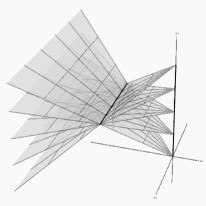
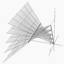
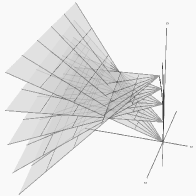
Figure 4: Left: When only $v_{y}\neq 0$, the camera becomes an orthogonal crossed-slit camera; middle: when $v_{x},v_{y}\neq 0$ are non-zero, the camera is a general crossed-slit camera; and right: when $\omega\neq 0$, the approximating camera is no longer a crossed-slit camera.

Thus, what a camera with a rolling-shutter becomes is a camera whose projection geometry is parameterized by its velocity. When stationary, the camera obeys the pinhole projection model. However, when undergoing linear motion with constant velocity, one can show that the camera becomes a crossed-slits camera. For any point $(u,v)$ we may invert (2.1) up to an unknown $z$ and demonstrate that all such inverse image coincide with two lines: the first being the line through $(0,0,0)$ and $(v_{x},v_{y},0)$; and the second through the points $(\pm 1,\frac{v_{0}v_{y}}{r},\frac{v_{y}}{r})$. As $v_{x}$ and $v_{y}$ approach $0$, these two slits coincide at $(0,0,0)$. The case when $\omega_{z}=v_{x}=0$ is shown in the left part of Figure 4; in the middle we show the case when $v_{x}$ and $v_{y}$ are arbitrary, and $\omega_{z}=0$; finally in the right part of Figure 4 we show that the resulting geometry when $\omega_{z}\neq 0$, in which case the camera no longer obeys the crossed-slits camera model.

2.2 Domain of applicability

Under what condition is the perspective model a sufficient model for rolling-shutter cameras? If error in feature location is on the order of one pixel, then we would expect distortions due to the rolling-shutter to be subsumed in noise. Thus, the maximum value that the correction term can obtain should be less than one pixel length in order for a perspective camera model to be an adequate representation of the rolling shutter camera. The correction term varies as a function of velocity and depth $z$. In order to determine when this correction term needs to be factored in, and a perspective model is no longer suitable, these parameters must be evaluated in light of the fixed parameters of the camera and the shutter rate $r$. Given that $s_{\alpha}$ is the length of a pixel, it can be seen that:

$$\frac{1}{s_{\alpha}r}v_{y}<z$$ (6)

must be satisfied in order for the rolling shutter effects to be inconsequential. However, when this inequality does not hold, then the rolling shutter projection model should be used or there will be a bias in estimations. This creates a limit line, as a function of $v_{y}$ and $z$, based on the shutter rate and $s_{\alpha}$, as shown in Figure5. When the values are such that the camera is operating well above this line, a rolling shutter model should be used.

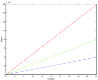
Figure 5: The limit line for a 640 x 480 image for different framerates. Blue represents 3.75fps, green is 7.5fps, and red is 15fps.

Case Solution to $t_{c}$ Projection equation Constant velocities $v=[v_{x},v_{y},0]$, $w=[0,0,w_{z}]$, and linear approximation of $P(t)$. Results in a linear equation which can be solved for $t_{c}$. Equation (2.1). Constant velocities $v=[0,0,v_{z}]$, $w=[0,0,0]$, and linear approximation of $P(t)$. Results in a quadratic equation for $t_{c}$, choose smallest positive root. The smallest positive root of $t_{c}$ when substituted into $q(t_{c})$ yields an analytic equation for the projection without $t_{c}$. Constant velocities $v=[v_{x},v_{y},v_{z}]$, $w=[w_{x},w_{y},w_{z}]$, and linear approximation of $P(t)$. Also results in a quadratic equation in $t_{c}$. Using the solution for $t_{c}$ in the general projection $q(t_{c})$ leads to a projection model is analytic and independent of $t_{c}$. Constant velocities $v=[v_{x},v_{y},v_{z}]$, $w=[w_{x},w_{y},w_{z}]$, without linear approximation of $P(t)$. Nonlinear equation for $t_{c}$; can be solved with a root finder (when $(x,y,z)$ are known). The projection equation $q(t_{c})$ is nonlinear in $t_{c}$.

Table 1: Different assumptions on the motion, and our choice in whether to linearize $P(t)$ lead to different types of solutions for $t_{c}$ and the projection $q(t_{c})$.

2.3 General rotation and translation

Generalizing the motion for any $T=[v_{x}v_{y}v_{z}]^{T}$ and an arbitrary rotation matrix $R$ we can see the relation of the rolling-shutter camera projection to $t_{c}$ for different. We discussed the linearity of the fronto-parallel case previously and can be see in (2.1). When there is a non-zero velocity along the principle axis of the camera, $v_{z}$, the relation now becomes quadratic. Using a root solver, we can find a solution of $t_{c}$ to make a rational projection equation. Different types of motion and the relation of the projection function to $t_{c}$ follow from the rolling-shutter rate (1) and (2). This relation and its effects on the projection are shown in Figure 1.

The linearized $P(t)$ and the resulting projection equation for rolling shutter camera can be used given any type of camera motion. In certain cases $t_{c}$ is a solution to a linear equation and in other cases, $t_{c}$ is a solution to a quadratic. In both instances $t_{c}$ can be found either directly or using a root solver and then used in the general projection equation to find a projection model of the rolling shutter that is independent of $t_{c}$. The resulting projection model will only be dependent on the velocity of the camera, the internal parameters, and the shutter rate.

3 Calibration

In this section we discuss the calibration of a Firewire camera with rolling shutter, namely the MDCS camera from Videre design. Our goal is to determine the constant $r$, the rate of scan, and determine if $d$, the delay between frames, is zero. If we find that $r=n_{r}/f$, where $n_{r}$ is the number of rows and $f$ is the framerate, then we can conclude that $d=0$.

Since the camera exposes only several neighboring scanlines at a time, we can indirectly measure $r$ by placing an LED flashing at known frequency in front of the camera and measuring the peak frequency of vertical slices of the image in the frequency domain. In a simple experiment we placed the camera in front of a green LED, removing its lens to ensure that all pixels are exposed by the LED, and draped a dark cloth over the setup so as to eliminate ambient light. An example of a captured image is shown in Figure 6; we were unable to achieve even distribution of exposure over the length of the scanline. For any choice of framerate and frequency, we selected and summed a subset of the columns from each image, yielding for any one time $t_{i}$ the vector $I(y,t_{i})$, thereby constructing an image $I(y,t)$ for each experiment whose independent variable is the pair of framerate and frequency. The duration of exposure, which is a configurable parameter, affects the width of the horizontal bars in Figure 6, though it does not affect their period. To estimate the frequency we take the two-dimensional Fourier transform of $I(y,t)$, obtaining $\hat{I}(\nu,\omega)$ which we marginalize over $\omega$ to yield $\tilde{I}(\nu)$. The estimate of $r$ is the location of the highest frequency peak (after high frequency components are ignored because the image is not a sine wave). Thus, using the image based frequency of the light flashes in conjunction with the actual frequency of the LED flashes from the pulse generator, we were able to approximate the rate of the rolling shutter for the camera. It can be seen in Figure 2 that it is sufficient to model our camera as having no delay .

FPS calibrated time ideal time (sec/row) (sec/row) 3.75 0.00110 $\pm$ 0.00050 0.00110 7.5 0.00063 $\pm$ 0.00050 0.00056 15 0.00029 $\pm$ 0.00050 0.00028

Table 2: The calibrated time to scan a row in relation to the ideal time to scan a row given the framerate. Note that the accuracy of the pulse generator frequency is taking into account in the offset number

Figure 6: Left: an example image taken during calibration; right: an example of the spatio-temporal image $I(y,t)$ used to estimate the rate $r$.

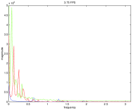
Figure 7: The positive frequencies of the marginalized 2D Fourier Transform of the LED capture image for framerate of 3.75 FPS. The blue shows the results using a pulse generator frequency(LED frequency) of 103Hz. The red shows the results for a pulse generator frequency of 20Hz. The green shows the results for pulse generator frequency of 11Hz.

3.1 Optical flow equations

To determine the optical flow equations for rolling-shutter cameras, we make the assumption that the parameterized camera can be sampled infinitely often in time. Furthermore, for ease of presentation we will assume from now on that $v_{0}=0$; in general this may induce some $t_{c}<0$. To determine the flow we solve the rolling-shutter constraint using the camera $P(t_{0}+t_{c})$, and having found and substituted $t_{c}$ as well as expressions for $x$ and $y$ in terms of the image coordinates and $z$, we differentiate with respect to $t_{0}$ and evaluate at $t_{0}=0$. For the case of fronto-parallel motion, i.e. $v=(v_{x},v_{y},0)^{T}$ and $\omega=(0,0,\omega_{z})$, and linearization of $t_{0}$, this procedure yields the following optical flow:

$$\dot{q}(u,v) = \frac{r\hskip 0.5ptz}{v\hskip 0.5ptv_{x}w_{z}+r\hskip 0.5ptz(r-\dot{v}_{p})}\begin{pmatrix}r\hskip 0.5pt\dot{u}_{p}+\omega_{z}v\hskip 0.5pt\dot{v}_{p}\\ r\hskip 0.5pt\dot{v}_{p}+\omega_{z}v\hskip 0.5pt\dot{u}_{p}\end{pmatrix},$$ (7)

where $(\dot{u}_{p},\dot{v}_{p})$ is the optical flow for perspective cameras in the case of fronto-parallel motion:

$$(\dot{u}_{p},\dot{v}_{p}) = \begin{bmatrix}\frac{v_{x}}{z}-\omega_{z}v,&\frac{v_{y}}{z}+\omega_{z}u\end{bmatrix}.$$

In the case of general motion and linearization of $P(t)$, the resulting equation for optical flow remains analytic but is significantly more complicated.

4 Simulation

\psfrag{DD}{\footnotesize{}Velocity: $1.875$ km/h.}\psfrag{CC}{\footnotesize{}Velocity: $3.75$ km/h.}\psfrag{BB}{\footnotesize{}Velocity: $5.625$ km/h.}\psfrag{AA}{\footnotesize{}Velocity: $7.5$ km/h.}\psfrag{PIXERR}{\tiny{}Simulated error (pixels)}\psfrag{QA}{\rotatebox{90.0}{\begin{minipage}{72.26999pt}\vspace{-3pt}\begin{center}\tiny{}Reprojection error\\ (for comparison only)\end{center}\end{minipage}}}\psfrag{QB}{\rotatebox{90.0}{\begin{minipage}{72.26999pt}\vspace{-3pt}\tiny{}Mean rotation \\ error (degrees)\end{minipage}}}\psfrag{QC}{\rotatebox{90.0}{\begin{minipage}{72.26999pt}\vspace{-3pt}\tiny{}Mean error in direction\\ of translation (degrees)\end{minipage}}}\includegraphics[scale={0.6}]{simfigs2.ps}

Figure 8: Plot of reprojection errors, errors in rotation and translation, and for varying velocities.

In section 2.2 we determined those conditions under which it may be wise to take into account distortions caused by a rolling shutter. In this section we test this claim in simulations under varying speeds and noise conditions. We randomly generate a set of $100$ points and project these points into two cameras according to the rolling-shutter camera model for certain $v_{y}\neq 0$, all others zero. The cameras are placed randomly, but on the order of $10$ meters from the point cloud. Then, assuming a camera sampling at $15$ frames per second, with scanning rate inversely proportional to the framerate, we let $v_{y}=1.875$, $3.75$, $5.625$ and $7.5$ km/h. For each velocity we perform experiments with pixel noises $\sigma=0.5$, $1.33$, $2.16$, $3$, $3.83$ and $4.66$ pixels.

For each instantiation of the experiment, we perform bundle adjustment on the image points using a projection model incorporating the rolling shutter (blue, solid lines) and the perspective projection model (red, dashed lines). The errors, plotted in Figure 8, are: left: reprojection error, middle: the error of the estimate $\hat{R}$ of rotation when compared with the true $R_{0}$, measured as $\|\log R_{0}^{-1}\hat{R}\|$; and, right: the error of the estimate $\hat{t}$ of translation when compared with the true $t_{0}$, measured as $\cos^{-1}\hat{t}^{T}t_{0}/(\|\hat{t}\|\,\|t_{0}\|)$.

For high velocities or low noise we find that by compensating for the rolling shutter, one is able to do better than if one were to ignore the effect. However, for lower velocities and higher noise, the noise effectively becomes louder, comparatively, than the deviation due to the rolling-shutter.

5 Conclusion

Despite the prevalence of rolling-shutter cameras little has been done to address the issues related to structure-from-motion. Since these cameras are becoming more common, the effects due to the shutter rate must be taken into account in vision systems. We have presented an analysis of the projective geometry of the rolling-shutter camera. In turn, we have derived the projection equation for such a camera and demonstrated that under certain conditions on the motion and internal parameters, using this flow equation can increase accuracy when doing structure-from-motion.

The effect of the rolling-shutter becomes important when either the camera or objects in the scene are moving, as the shutter rate can produce distortion if not accounted for. The modeling we have presented may play an important role for incorporating rolling-shutter cameras into moving systems, such as UAV’s and ground robots. Given the improved accuracy in structure-from-motion, this can aid in scene recovery and navigation of systems operating in dynamic worlds. Future work includes testing these models on UAV’s for recovery of scene structure.

References

- [1] 1394 Trade Association. IIDC 1394-based Digital Camera Specification Ver.1.30. July 2000.
- [2] D. Feldman, T. Pajdla, and D. Weinshall. On the epipolar geometry of the crossed-slits projection. In Proceedings of International Conference on Computer Vision, pages 988 – 995, October 2003.
- [3] R. Hartley and R. Gupta. Linear pushbroom cameras. In Proceedings of European Conference on Computer Vision, 1994.
- [4] R. Hartley and A. Zisserman. Multiple View Geometry. Cambridge Univ. Press, 2000.
- [5] M. Latzel and J. K. Tsotso. A robust motion detection and estimation filter for video signals. In Proceedings of Image Processing, pages 381 – 394, October 2001.
- [6] Y. Ma, S. Soatto, J. Košecká, and S. Sastry. An Invitiation to 3D Vision: From Images to Geometric Models. Springer Verlag, New York, 2003.
- [7] T. Pajdla. Geometry of two-slit camera. Czech Technical University, Technical report CTU-CMP-2002-02, 2002.
- [8] R. Pless. Discrete and differential two-view constraints for general imaging systems. In Proceedings of the 3rd Workshop on Omnidirectional Vision, June 2002.
- [9] M. Wäny and G. P. Israel. CMOS image sensor with NMOS-only global shutter and enhanced responsivity. Trans. on Electron Devices, 50(1), January 2003.
- [10] B. Wilburn, N. Joshi, V. Vaish, M. Levoy, and M. Horowitz. High speed video using a dense camera array. In Proceedings of Computer Vision and Pattern Recognition, 2004.
- [11] J. Yu and L. McMillan. General linear cameras. In Proceedings of European Conference on Computer Vision, 2004.
- [12] A. Zomet, D. Feldman, S. Peleg, and D. Weinshall. Mosaicing new views: the crossed-slits projection. Trans. on Pattern Analysis and Machine Intelligence, 25(6), June 2003.