Randomly Spread CDMA: Asymptotics via Statistical Physics

Abstract

This paper studies randomly spread code-division multiple access (CDMA) and multiuser detection in the large-system limit using the replica method developed in statistical physics. Arbitrary input distributions and flat fading are considered. A generic multiuser detector in the form of the posterior mean estimator is applied before single-user decoding. The generic detector can be particularized to the matched filter, decorrelator, linear MMSE detector, the jointly or the individually optimal detector, and others. It is found that the detection output for each user, although in general asymptotically non-Gaussian conditioned on the transmitted symbol, converges as the number of users go to infinity to a deterministic function of a “hidden” Gaussian statistic independent of the interferers. Thus the multiuser channel can be decoupled: Each user experiences an equivalent single-user Gaussian channel, whose signal-to-noise ratio suffers a degradation due to the multiple-access interference. The uncoded error performance (e.g., symbol-error-rate) and the mutual information can then be fully characterized using the degradation factor, also known as the multiuser efficiency, which can be obtained by solving a pair of coupled fixed-point equations identified in this paper. Based on a general linear vector channel model, the results are also applicable to MIMO channels such as in multiantenna systems.

I Introduction

Consider a multidimensional Euclidean space in which each user (or data stream) randomly selects a “signature vector” and modulates its own information-bearing symbols onto it for transmission. The received signal is a superposition of all users’ signals corrupted by Gaussian noise. Such a multiuser scheme, best described by a vector channel model, is very versatile and is widely used in applications that include code-division multiple access (CDMA), as well as certain multi-input multi-output (MIMO) systems. With knowledge of all signature vectors, the goal is to estimate the transmitted symbols and eventually recover the information intended for all or a subset of the users.

This paper focuses on a paradigm of multiuser channels, known as randomly spread CDMA [1]. In such a CDMA system, a number of users share a common media to communicate to a single receiver simultaneously over the same bandwidth. Each user employs a randomly generated spreading sequence (signature waveform) with a large time-bandwidth product. This multiaccess method has many advantages particularly in wireless communications: frequency diversity, robustness to channel impairments, ease of resource allocation, etc. The price to pay is multiple-access interference (MAI) due to non-orthogonal spreading sequences from all users. Numerous multiuser detection techniques have been proposed to mitigate the MAI to various degrees. This work is concerned with the performance of such multiuser systems in two aspects: 1) Uncoded symbol-error-rate (or equivalently, multiuser efficiency) and 2) Spectral efficiency, namely the total information rate achievable by coded transmission and normalized by the dimension of the multiuser channel.

I-A Gaussian or Non-Gaussian?

The most efficient use of a multiuser channel is through jointly optimal decoding, which is prohibitively complex with a large population of users. Although suboptimal, the philosophy of separating the tasks of untangling the mutually interference streams and exploiting the redundancy in the coded streams has received much attention. A multiuser detection front end supplies individual (hard or soft) decision statistics to independent single-user decoders. With the exception of decorrelating receivers, the multiuser detector outputs are still contaminated by multiaccess interference, and their statistical characterization is of paramount interest.

In [2, 3, 4], Verdú first used the concept of multiuser efficiency to refer to the degradation of the output signal-to-noise ratio (SNR) relative to a single-user channel calibrated at the same bit-error-rate (BER) in binary (antipodal) uncoded transmission. The multiuser efficiencies of the single-user matched filter, decorrelator, and linear minimum mean-square error (MMSE) detector were found as functions of the correlation matrix of the spreading sequences. Particular attention has been given to the asymptotic multiuser efficiency in the more tractable region of high SNR. Expressions for the optimum (high-SNR) asymptotic multiuser efficiency were found in [4, 5].

In the large-system limit, where the number of users and the spreading factor both tend to infinity with a fixed ratio, the dependence of system performance on the sequences vanishes, and random matrix theory proves to be a capable tool for analyzing linear detectors. The limiting multiuser efficiency of the matched filter is trivial [1]. The large-system multiuser efficiency of the linear MMSE detector is obtained explicitly in [1] for the equal-power case (perfect power control), and in [6] for the case with flat fading as the solution to the Tse-Hanly fixed-point equation. The efficiency of the decorrelator is also known [1, 7, 8]. The success of the multiuser efficiency analysis of the wide class of linear detectors hinges on the fact that 1) the detection output is a sum of independent components: the desired signal, the MAI and Gaussian background noise, e.g., the decision statistic for user $k$ is

$$\left\langle X_{k}\right\rangle=X_{k}+I_{k}+N_{k};$$ (1)

and 2) the multiple-access interference ($I_{k}$) is asymptotically Gaussian (e.g., [9]). As far as linear multiuser detectors are concerned, regardless of the input distribution, the performance is fully characterized by the noise enhancement associated with the MAI variance. Indeed, by regarding the multiuser detector as part of the channel, an individual user experiences asymptotically a single-user Gaussian channel with an SNR degradation equal to the multiuser efficiency.

The performance analysis of nonlinear detectors such as the optimal ones is a hard problem. The difficulty here is inherent to nonlinear operations: The detection output cannot be decomposed as a sum of independent components associated with the desired signal, the interferences and the noise respectively. Moreover, the detection output is in general asymptotically non-Gaussian conditioned on the input. An extreme case is the maximum-likelihood multiuser detector for binary transmission, the hard decision output of which takes only two values. The difficulty remains even if we consider soft detection outputs. Hence, unlike for a Gaussian output statistic, the conditional variance of a general detection output does not lead to a simple characterization of the multiuser efficiency or error performance. For illustration, Figure 1 plots the approximate probability density function obtained from the histogram of the soft output statistic of the individually optimal detector conditioned on $+1$ being transmitted. The simulated system has 8 users with binary inputs, a spreading factor of 12, and SNR=2 dB. A total of 10,000 trials were recorded. Note that negative decision values correspond to decision error; hence the area under the curve on the negative half plane gives the BER. The distribution shown in Figure 1 is far from Gaussian. Thus the usual notion of output SNR fails to capture the essence of system performance. In fact, much literature is devoted to evaluating the error performance by Monte Carlo simulation.

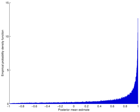
Figure 1: The empirical probability density function of the individually optimal soft detection output conditioned on $+1$ being transmitted. The system has 8 users, the spreading factor is 12, and SNR=2 dB.

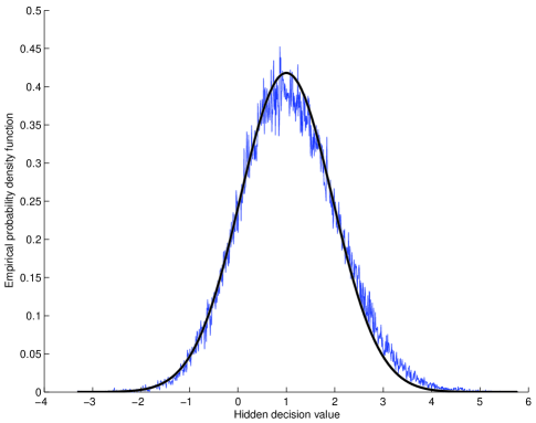
Figure 2: The empirical probability density function of the hidden equivalent Gaussian statistic conditioned on $+1$ being transmitted. The system has 8 users, the spreading factor is 12, and SNR=2 dB. The asymptotic Gaussian distribution is also plotted for comparison.

This paper makes a contribution to the understanding of multiuser detection in the large-system regime. It is found under certain assumptions that the output decision statistic of a nonlinear detector, such as the one whose distribution is depicted by Figure 1, converges in fact to a very simple monotone function of a “hidden” conditionally Gaussian random variable, i.e.,

$$\left\langle X_{k}\right\rangle\rightarrow f(Z_{k})$$ (2)

where $Z_{k}=X_{k}+N^{\prime}_{k}$ and $N^{\prime}_{k}$ is Gaussian. One may contend that it is always possible to monotonically map a non-Gaussian random variable to a Gaussian one. What is surprisingly simple and useful here is that 1) the mapping $f$ neither depends on the instantaneous spreading sequences, nor on the transmitted symbols which we wish to estimate in the first place; and 2) the statistic $Z_{k}$ is equal to the desired signal plus an independent Gaussian noise. Indeed, a few parameters of the system determine the function $f$. By applying an inverse of this function to the detection output $\left\langle X_{k}\right\rangle$, an equivalent conditionally Gaussian statistic $Z_{k}$ is recovered, so that we are back to the familiar ground where the output SNR (defined for the equivalent Gaussian statistic $Z_{k}$) completely characterizes the system performance. The multiuser efficiency is simply obtained as the ratio of the output and input SNRs. We will refer to this result as the “decoupling principle” since asymptotically, after applying $f^{-1}$, each user’s data goes through an equivalent single-user channel with an additive Gaussian noise which is independent of the interferers’ data.

Under certain assumptions, we show the decoupling principle to hold for not only optimal detection, but also a broad family of generic multiuser detectors, called the posterior mean estimators (PME), which compute the mean value of the input conditioned on the observation assuming a certain postulated posterior probability distribution. Simply put, the generic detector is the optimal detector for a postulated multiuser system that may be different from the actual one. In case the postulated posterior is identical to the one induced by the actual multiuser channel and input, the PME is a soft version of the individually optimal detector. The postulated posterior, however, can also be chosen such that the resulting PME becomes one of many other detectors, including but not limited to the matched filter, decorrelator, linear MMSE detector, as well as the jointly optimal detector. Moreover, the decoupling principle holds for not only binary inputs, but arbitrary input distributions with finite power.

For illustration of the new findings, Figure 2 plots the approximate probability density function obtained from the histogram of the conditionally Gaussian statistic obtained by applying $f^{-1}$ to the non-Gaussian detection output in Figure 1. The theoretically predicted Gaussian density function is also shown for comparison. The “fit” is good considering that a relatively small system of 8 users with a processing gain of 12 is considered. Note that in case the multiuser detector is linear, the mapping $f$ is also linear, and (2) reduces to (1).

By virtue of the decoupling principle, the mutual information between the input and the output of the generic detector for each user converges to the input-output mutual information of the equivalent single-user Gaussian channel under the same input, which admits a simple analytical expression. Hence the large-system spectral efficiency of several well-known linear detectors, first found in [10] and [11] with and without fading respectively, can be recovered straightforwardly using the decoupling principle. New results on the spectral efficiency of nonlinear detection and arbitrary inputs under both joint and separate decoding are also obtained. Furthermore, the additive decomposition of optimal spectral efficiency as a sum of single-user efficiencies and a joint decoding gain [11] applies under more general conditions than originally thought.

As in random matrix spectrum analysis, our large-system results are representative of the behavior of systems of moderate size. As shown in Figures 1 and 2, a randomly spread system with as few as 8 users can often be well approximated by the large-system limiting results.

I-B Random Matrix vs. Spin Glass

Much of the early success in the large-system analysis of linear detectors relies on the fact that the multiuser efficiency of a finite-size system can be written as an explicit function of the eigenvalues of the correlation matrix of the random signature waveforms, the empirical distributions of which converge to a known function in the large-system limit [12, 13]. As a result, the large-system multiuser efficiency can be obtained as an integral with respect to the limiting eigenvalue distribution. Indeed, this random matrix technique is applicable to any performance measure that can be expressed as a function of the eigenvalues. Based on an explicit expression for CDMA channel capacity in [14], Verdú and Shamai quantified the optimal spectral efficiency in the large-system limit [10, 11] (see also [15, 16]). The expression found in [10] also solved the capacity of single-user narrowband multiantenna channels as the number of antennas grows—a problem that was open since the pioneering work of Foschini [17] and Telatar [18]. Unfortunately, few explicit expressions of the efficiencies in terms of eigenvalues are available beyond the above cases. Much less success has been reported in the application of random matrix theory when either the detector is nonlinear or the inputs are non-Gaussian constellations.

A major consequence of random matrix theory is that the dependence of performance measures on the spreading sequences vanishes as the system size increases without bound. In other words, the performance measures are “self-averaging.” In the context of physical science, this property is nothing but a manifestation of a fundamental law that the fluctuation of macroscopic properties of certain many-body systems vanishes in the thermodynamic limit, i.e., when the number of interacting bodies becomes large. This falls under the general scope of statistical mechanics (aka statistical physics), whose principal goal is to study the macroscopic properties of physical systems from the principle of microscopic interactions. Indeed, the asymptotic eigenvalue distribution of certain correlation matrices can be derived via statistical physics (e.g., [19]). Tanaka pioneered the user of statistical physics concepts and methodologies in multiuser detection and obtained the large-system uncoded minimum BER (hence the optimal multiuser efficiency) and spectral efficiency with equal-power binary inputs [20, 21, 22, 23]. In [8] we further elucidated the relationship between CDMA and statistical physics and generalized to the case of unequal powers. Inspired by [23], Müller and Gerstacker [24] studied the channel capacity under separate decoding and noticed that the additive decomposition of the optimum spectral efficiency in [11] holds also for binary inputs. Müller thus further conjectured the same formula to be valid regardless of the input distribution [25].

In this paper, we build upon Tanaka’s ground-breaking contribution [23] and present a unified treatment of Gaussian CDMA channels and multiuser detection assuming an arbitrary input distribution and flat fading characteristic. A wide class of multiuser detectors, optimal as well as suboptimal, are studied under the same umbrella of posterior mean estimation. The central results are the decoupling principle for generic multiuser detection, the characterization of multiuser efficiency via a pair of nonlinear equations, as well as the spectral efficiencies of separate and joint decoding.

The key tool in this paper, the replica method, has its origin in spin glass theory [26]. Analogies between statistical physics and neural networks, coding, image processing, and communications have long been noted (e.g., [27, 28]). There have been many recent activities applying statistical physics wisdom to sparse-graph error-correcting codes (e.g., [29, 30, 31, 32, 33]). Similar techniques have also been used to study capacity of MIMO channels [34]. Among others, mean field theory is used to derive iterative detection algorithms [35, 36]. The first application of the replica method to multiuser detection was made in [23]. In this paper, we draw a parallel between the general statistical inference problem in multiuser communications and the problem of determining the configuration of random spins subject to quenched randomness. For the purpose of analytical tractability, we will invoke common assumptions in the statistical physics literature: 1) the self-averaging property applies, 2) the “replica trick” is valid, and 3) replica symmetry holds. These assumptions have been used successfully in many problems in statistical physics as well as in neural networks and coding theory, to name a few, while a complete justification of the replica method is a notoriously difficult challenge in mathematical physics, which has seen some important progress recently [37, 38]. The results in this paper are based on the aforementioned assumptions and therefore the mathematical rigor is pending on breakthroughs in those problems. A set of easy-to-check sufficient conditions under which the replica method is justified is yet to be found. In statistical physics it has been found that results obtained using the replica method may still capture many of the qualitative features of the system performance even when the key assumptions fail [39, 40]. Furthermore, the decoupling principle carries great practicality and finds convenient uses in finite-size systems where the analytical asymptotic results are a good approximation.

The remainder of this paper is organized as follows. Section II gives the model and summarizes the main results. Relevant statistical physics concepts and methodologies are introduced in Section III. Calculations based on a real-valued channel are presented in Section IV. Complex-valued channels are discussed in Section V, followed by some numerical examples in Section VI. Some conclusions are drawn in Section VII.

II Model and Summary of Results

II-A System Model

Figure 3: A multiuser system with joint decoding.

Consider the synchronous $K$-user CDMA system with spreading factor $L$ as depicted in Figure 3. Each encoder maps its message into a sequence of channel symbols. All users employ the same type of signaling so that at each interval the $K$ symbols are independent identically distributed (i.i.d.) random variables with distribution (probability measure) $P_{X}$, which has zero mean and unit variance. Let ${\boldsymbol{X}}=[X_{1},\dots,X_{K}]^{\!\top\!}$ denote the vector of input symbols from the $K$ users in one symbol interval. For notational convenience in the analysis, it is assumed that either a probability density function or a probability mass function of $P_{X}$ exists, and is denoted by $p_{X}$. Let also $p_{\boldsymbol{X}}({\boldsymbol{x}})=\prod^{K}_{k=1}p_{X}(x_{k})$ denote the joint (product) distribution.

Let the instantaneous SNR of user $k$ be denoted by ${\mathsf{snr}}_{k}$ and ${\boldsymbol{A}}=\text{diag}\{\sqrt{{\mathsf{snr}}_{1}}\,,\dots,\sqrt{{\mathsf{snr}}_{K}}\,\}$. Denote the spreading sequence of user $k$ by ${\boldsymbol{s}}_{k}=\frac{1}{\sqrt{L}}[S_{1k},S_{2k},\dots,S_{Lk}]^{\!\top\!}$, where $S_{nk}$ are i.i.d. random variables with zero mean and finite moments. Let the symbols and spreading sequences be randomly chosen for each user and not dependent on the SNRs. The $L\times K$ channel “state” matrix is denoted by ${\boldsymbol{S}}=[\sqrt{{\mathsf{snr}}_{1}}\,{\boldsymbol{s}}_{1},\dots,\sqrt{{\mathsf{snr}}_{K}}\,{\boldsymbol{s}}_{K}]$. The synchronous CDMA channel with flat fading is described by:

$${\boldsymbol{Y}} = \sum^{K}_{k=1}\sqrt{{\mathsf{snr}}_{k}}\,{\boldsymbol{s}}_{k}X_{k}+{\boldsymbol{N}}$$ (3)

$$= {\boldsymbol{S}}{\boldsymbol{X}}+{\boldsymbol{N}}$$ (4)

where ${\boldsymbol{N}}$ is a vector consisting of i.i.d. zero-mean Gaussian random variables. Depending on the domain that the inputs and spreading chips take values, the input-output relationship (4) describes either a real-valued or a complex-valued fading channel.

The linear system (4) is quite versatile. In particular, with ${\mathsf{snr}}_{k}={\mathsf{snr}}$ for all $k$, it models the canonical MIMO channel in which all propagation coefficients are i.i.d. An example is single-user communication with $K$ transmit antennas and $L$ receive antennas, where the channel coefficients are not known to the transmitter.

II-B Posterior Mean Estimation

Figure 4: Multiuser detection followed by independent single-user decoding.

The information-bearing symbol (vector) ${\boldsymbol{X}}$ is drawn according to the prior distribution $p_{\boldsymbol{X}}$. The channel response to the input ${\boldsymbol{X}}$ is an output ${\boldsymbol{Y}}$ generated according to a conditional probability distribution $p_{{\boldsymbol{Y}}|{\boldsymbol{X}},{\boldsymbol{S}}}$ where ${\boldsymbol{S}}$ is the channel state. Upon receiving ${\boldsymbol{Y}}$, the estimator would like to infer the transmitted symbol ${\boldsymbol{X}}$ with knowledge of ${\boldsymbol{S}}$.

The most efficient use of the multiuser channel (4) is achieved by optimal joint decoding as depicted in Figure 3. Due to the complexity of joint decoding, the processing is often separated into multiuser detection followed by single-user error-control decoding as shown in Figure 4. A multiuser detector front end estimates the transmitted symbols given the received signal and the channel state, without using any knowledge of the error-control codes employed by the transmitters. Conversely, each single-user decoder only observes the sequence of decision statistics corresponding to one user, and does not take into account the existence of any other users (in particular, it does not use any knowledge of the spreading sequences). By adopting this separate decoding approach, the channel together with the multiuser detector front end is viewed as a bank of coupled single-user channels. The detection output sequence for an individual user is in general not a sufficient statistic for decoding this user’s own information.

To capture the intended suboptimal structure, one has to restrict the capability of the multiuser detector; otherwise the detector could in principle encode the channel state and the received signal $({\boldsymbol{S}},{\boldsymbol{Y}})$ into a single real number as its output to each user, which is a sufficient statistic for all users. A plausible choice is the (canonical) posterior mean estimator, which computes the mean value of the posterior probability distribution $p_{{\boldsymbol{X}}|{\boldsymbol{Y}},{\boldsymbol{S}}}$, hereafter denoted by angle brackets $\left\langle\cdot\right\rangle$:

$$\left\langle{\boldsymbol{X}}\right\rangle={\mathsf{E}}\left\{\left.{\boldsymbol{X}}\,\right|\,{\boldsymbol{Y}},{\boldsymbol{S}}\right\}.$$ (5)

Also known as the conditional mean estimator, this estimator achieves the minimum mean-square error for each user, and is therefore the (nonlinear) MMSE detector. We also regard it as a soft-output version of the individually optimal multiuser detector (assuming uncoded transmission). The posterior probability distribution $p_{{\boldsymbol{X}}|{\boldsymbol{Y}},{\boldsymbol{S}}}$ is induced from the input distribution $p_{\boldsymbol{X}}$ and the conditional Gaussian density function $p_{{\boldsymbol{Y}}|{\boldsymbol{X}},{\boldsymbol{S}}}$ of the channel (4) by the Bayes formula:

$$p_{{\boldsymbol{X}}|{\boldsymbol{Y}},{\boldsymbol{S}}}({\boldsymbol{x}}|{\boldsymbol{y}},{\boldsymbol{S}})=\frac{p_{{\boldsymbol{X}}}({\boldsymbol{x}})p_{{\boldsymbol{Y}}|{\boldsymbol{X}},{\boldsymbol{S}}}({\boldsymbol{y}}|{\boldsymbol{x}},{\boldsymbol{S}})}{\int p_{{\boldsymbol{X}}}({\boldsymbol{x}})p_{{\boldsymbol{Y}}|{\boldsymbol{X}},{\boldsymbol{S}}}({\boldsymbol{y}}|{\boldsymbol{x}},{\boldsymbol{S}})\,{\,{\text{d}}}{\boldsymbol{x}}}.$$ (6)

The PME can be understood as an “informed” optimal estimator which is supplied with the posterior distribution $p_{{\boldsymbol{X}}|{\boldsymbol{Y}},{\boldsymbol{S}}}$ and then computes its mean. A generalization of the canonical PME is conceivable: Instead of informing the estimator with the actual posterior $p_{{\boldsymbol{X}}|{\boldsymbol{Y}},{\boldsymbol{S}}}$, we can supply at will any other well-defined conditional distribution $q_{{\boldsymbol{X}}|{\boldsymbol{Y}},{\boldsymbol{S}}}$. Given $({\boldsymbol{Y}},{\boldsymbol{S}})$, the estimator can nonetheless perform “optimal” estimation based on this postulated measure $q$. We call this the generalized posterior mean estimation, which is conveniently denoted as

$$\left\langle{\boldsymbol{X}}\right\rangle_{q}={\mathsf{E}_{q}}\left\{\left.{\boldsymbol{X}}\,\right|\,{\boldsymbol{Y}},{\boldsymbol{S}}\right\}$$ (7)

where $\mathsf{E}_{q}\{\cdot\}$ stands for the expectation with respect to the postulated measure $q$. For brevity, we will also refer to (7) by the name of the posterior mean estimator, or simply the PME. In view of (5), the subscript in (7) can be dropped if the postulated measure $q$ coincides with the actual one $p$.

In general, postulating $q\neq p$ causes degradation in detection performance. Such a strategy may be either due to lack of knowledge of the true statistics or a particular choice that corresponds to a certain estimator of interest. In principle, any deterministic estimation can be regarded as a PME since we can always choose to put a unit mass at the desired estimation output given $({\boldsymbol{Y}},{\boldsymbol{S}})$. We will see in Section II-C that by postulating an appropriate measure $q$, the PME can be particularized to many important multiuser detectors. As will also be shown in this paper, the generic representation (7) allows a uniform treatment of a large family of multiuser detectors which results in a simple performance characterization for all of them.

It is enlightening to introduce a new concept: the retrochannel, which is defined for a given channel and input as a companion channel in the opposite direction characterized by a posterior distribution. Given the multiuser channel $p_{{\boldsymbol{Y}}|{\boldsymbol{X}},{\boldsymbol{S}}}$ with an input $p_{\boldsymbol{X}}$, we have a (canonical) retrochannel defined by $p_{{\boldsymbol{X}}|{\boldsymbol{Y}},{\boldsymbol{S}}}$ (6), which, upon an input $({\boldsymbol{Y}},{\boldsymbol{S}})$, generates a random output ${\boldsymbol{X}}$ according to $p_{{\boldsymbol{X}}|{\boldsymbol{Y}},{\boldsymbol{S}}}$. A retrochannel in the single-user setting is similarly defined. In general, any valid posterior distribution $q_{{\boldsymbol{X}}|{\boldsymbol{Y}},{\boldsymbol{S}}}$ can be regarded as a retrochannel. Note that the retrochannel samples from the Bayesian posterior distribution (in general, the postulated one) in such a way that, conditioned on the observation, the input to the channel and the output of the retrochannel are independent. It is clear that the PME output $\left\langle{\boldsymbol{X}}\right\rangle_{q}$ is the expected value of the output of the retrochannel $q_{{\boldsymbol{X}}|{\boldsymbol{Y}},{\boldsymbol{S}}}$ given $({\boldsymbol{Y}},{\boldsymbol{S}})$.

In this paper, the posterior $q_{{\boldsymbol{X}}|{\boldsymbol{Y}},{\boldsymbol{S}}}$ supplied to the PME is assumed to be the one that corresponds to a postulated CDMA system, where the input distribution is an arbitrary $q_{X}$, and the input-output relationship of the postulated channel differs from the actual channel (4) by only the noise variance. Precisely, the postulated channel is characterized by

$${\boldsymbol{Y}}={\boldsymbol{S}}{\boldsymbol{X}}^{\prime}+\sigma{\boldsymbol{N}}^{\prime}$$ (8)

where the channel state matrix ${\boldsymbol{S}}$ is identical to that of the actual channel (4), and ${\boldsymbol{N}}^{\prime}$ is statistically the same as the Gaussian noise ${\boldsymbol{N}}$ in (4). The postulated input distribution $q_{X}$ is assumed to have zero-mean and finite moments, and $q_{{\boldsymbol{X}}|{\boldsymbol{Y}},{\boldsymbol{S}}}$ is determined by $q_{X}$ and $q_{{\boldsymbol{Y}}|{\boldsymbol{X}},{\boldsymbol{S}}}$ according to the Bayes formula. Here, $\sigma$ serves as a control parameter. Indeed, the PME so defined is the optimal detector for a postulated multiuser system with its input distribution and noise level different from the actual ones. In general, the assumed information about the channel state ${\boldsymbol{S}}$ could also be different from the actual instances, but this is out of the scope of this work, as we limit ourselves to study the (rich) family of multiuser detectors that can be represented as the PME parameterized by the postulated input and noise level $(q_{X},\sigma)$.

We note that PME under postulated posterior is known in the Bayes statistics literature. This technique was introduced to multiuser detection by Tanaka in the special case of equal-power users with binary or Gaussian inputs under the name of marginal-posterior-mode detectors [20, 23]. In this paper we pursue further that direction to treat arbitrary input, arbitrary power distribution, and generic multiuser detection.

II-C Specific Detectors

The rest of this section assumes the system model (4) to be real-valued. The inputs $X_{k}$, the spreading chips $S_{nk}$, and all entries of ${\boldsymbol{N}}$ take real values and have unit variance. The characteristic of the actual channel is

$$p_{{\boldsymbol{Y}}|{\boldsymbol{X}},{\boldsymbol{S}}}({\boldsymbol{y}}|{\boldsymbol{x}},{\boldsymbol{S}})=(2\pi)^{-\frac{L}{2}}\exp\left[-\frac{\|{\boldsymbol{y}}-{\boldsymbol{S}}{\boldsymbol{x}}\|^{2}}{2}\right],$$ (9)

and that of the postulated channel is

$$q_{{\boldsymbol{Y}}|{\boldsymbol{X}},{\boldsymbol{S}}}({\boldsymbol{y}}|{\boldsymbol{x}},{\boldsymbol{S}})=\left(2\pi\sigma^{2}\right)^{-\frac{L}{2}}\exp\left[-\frac{\|{\boldsymbol{y}}-{\boldsymbol{S}}{\boldsymbol{x}}\|^{2}}{2\sigma^{2}}\right].$$ (10)

We identify specific choices of the postulated input distribution $q_{X}$ and noise level $\sigma$ under which the PME is particularized to well-known multiuser detectors.

II-C1 Linear Detectors

Let the postulated input be standard Gaussian, $q_{X}\sim\mathcal{N}(0,1)$. The optimal detector (PME) for the postulated model (8) with standard Gaussian inputs is a linear filtering of the received signal ${\boldsymbol{Y}}$:

$$\left\langle{\boldsymbol{X}}\right\rangle_{q}=\left[{\boldsymbol{S}}^{\!\top\!}{\boldsymbol{S}}+\sigma^{2}{\boldsymbol{I}}\right]^{\scriptscriptstyle-\!1}\,{\boldsymbol{S}}^{\!\top\!}\,{\boldsymbol{Y}}.$$ (11)

The control parameter $\sigma$ can be tuned to choose from the single-user matched filter, decorrelator, MMSE detector, etc. If $\sigma\rightarrow\infty$, the PME estimate (11) is consistent with the single-user matched filter output:

$$\sigma^{2}\,\left\langle X_{k}\right\rangle_{q}\longrightarrow{\boldsymbol{s}}^{\!\top\!}_{k}\,{\boldsymbol{Y}},\quad\text{in }L^{2}\text{ as }\sigma\rightarrow\infty.$$ (12)

If $\sigma=1$, (11) is exactly the soft output of the linear MMSE detector. If $\sigma\rightarrow 0$, (11) converges to the decorrelator output.

II-C2 Optimal Detectors

Let the postulated $q_{X}$ be identical to the true one, $p_{X}$. The posterior is then

$$q_{{\boldsymbol{X}}|{\boldsymbol{Y}},{\boldsymbol{S}}}({\boldsymbol{x}}|{\boldsymbol{y}},{\boldsymbol{S}})=\frac{p_{\boldsymbol{X}}({\boldsymbol{x}})}{Z({\boldsymbol{y}},{\boldsymbol{S}})}\,\exp\left[{-\frac{1}{2\sigma^{2}}\|{\boldsymbol{y}}-{\boldsymbol{S}}{\boldsymbol{x}}\|^{2}}\right]$$ (13)

where $Z({\boldsymbol{y}},{\boldsymbol{S}})$ is a normalization factor.

Suppose that the postulated noise level $\sigma\rightarrow 0$, then the probability mass of the distribution $q_{{\boldsymbol{X}}|{\boldsymbol{Y}},{\boldsymbol{S}}}$ is concentrated on a vector that minimizes $\|{\boldsymbol{y}}-{\boldsymbol{S}}{\boldsymbol{x}}\|$, which also maximizes the likelihood function $p_{{\boldsymbol{Y}}|{\boldsymbol{X}},{\boldsymbol{S}}}({\boldsymbol{y}}|{\boldsymbol{x}},{\boldsymbol{S}})$. The PME $\lim_{\sigma\rightarrow 0}\left\langle{\boldsymbol{X}}\right\rangle_{q}$ is thus equivalent to that of jointly optimal (or maximum-likelihood) detection [1].

Alternatively, if $\sigma=1$, then the postulated measure coincides with the actual measure, i.e., $q=p$. The PME output $\left\langle{\boldsymbol{X}}\right\rangle$ is the mean of the marginal of the conditional posterior probability distribution. It is the nonlinear MMSE detector for the actual system, and is seen as a soft version of the individually optimal detector [1].

Also worth mentioning here is that, if $\sigma\rightarrow\infty$, the PME reduces to the single-user matched filter. Indeed, (12) can be shown to hold by noticing from (13) that

$$q_{{\boldsymbol{X}}|{\boldsymbol{Y}},{\boldsymbol{S}}}({\boldsymbol{x}}|{\boldsymbol{y}},{\boldsymbol{S}})=p_{{\boldsymbol{X}}}({\boldsymbol{x}})\left[1-\frac{\|{\boldsymbol{y}}-{\boldsymbol{S}}{\boldsymbol{x}}\|^{2}}{2\sigma^{2}}+\mathcal{O}\Big{(}\frac{1}{\sigma^{4}}\Big{)}\right].$$ (14)

II-D Main Results

This subsection gives the main results of this paper assuming the real-valued system model. The detailed replica analysis for obtaining these results is relegated to Sections III and IV. Results for a complex-valued model are given in Section V.

Consider the multiuser channel $p_{{\boldsymbol{Y}}|{\boldsymbol{X}},{\boldsymbol{S}}}$ given by (9) with input ${\boldsymbol{X}}\sim p_{\boldsymbol{X}}$, and the posterior mean estimator (7) parameterized by $(q_{X},\sigma)$. Section II-C illustrated the versatility of the PME encompassing many well-known detectors. The goal here is to quantify the optimal spectral efficiency $\frac{1}{L}I({\boldsymbol{X}};{\boldsymbol{Y}}|{\boldsymbol{S}})$, the quality of the detection output $\left\langle X_{k}\right\rangle_{q}$ for each user $k$, as well as the input-output mutual information $I(X_{k};\left\langle X_{k}\right\rangle_{q}|{\boldsymbol{S}})$.

Although these performance measures are all dependent on the realization of the channel state, such dependence vanishes in the large-system asymptote. A large system here refers to the limit that both the number of users and the spreading factor tend to infinity but with their ratio, known as the system load, converging to a positive number, i.e., $K/L\rightarrow\beta$, which may or may not be smaller than 1. It is also assumed that the SNRs of all users, $\{{\mathsf{snr}}_{k}\}^{K}_{k=1}$, are i.i.d. with distribution $P_{\mathsf{snr}}$, hereafter referred to as the SNR distribution. All moments of the SNR distribution are assumed to be finite. Clearly, the empirical distributions of the SNRs converge to the same distribution $P_{\mathsf{snr}}$ as $K\rightarrow\infty$. Note that this SNR distribution captures the (flat) fading characteristics of the channel.

Given $(\beta,P_{\mathsf{snr}},p_{X},q_{X},\sigma)$, we express the large-system limit of the multiuser efficiency and spectral efficiency under both separate and joint decoding.

II-D1 The Decoupling Principle

Figure 5: (a) The multiuser channel, the (multiuser) PME, and the companion (multiuser) retrochannel. (b) The equivalent single-user Gaussian channel, PME and retrochannel.

The multiuser channel $p_{{\boldsymbol{Y}}|{\boldsymbol{X}},{\boldsymbol{S}}}$ and the multiuser posterior mean estimator parameterized by $(q_{X},\sigma)$ are depicted in Figure 5, together with the companion (multiuser) retrochannel $q_{{\boldsymbol{X}}|{\boldsymbol{Y}},{\boldsymbol{S}}}$. Here the input to the multiuser channel is denoted by ${\boldsymbol{X}}_{0}$ to distinguish from the output ${\boldsymbol{X}}$ of the retrochannel. For an arbitrary user $k$, the SNR is ${\mathsf{snr}}_{k}$, and $X_{0k}$, $X_{k}$ and $\left\langle X_{k}\right\rangle_{q}$ denote the input symbol, the retrochannel output and the PME output, all for user $k$.

In order to show the decoupling result, let us also consider the composition of a Gaussian channel, a PME and a companion retrochannel in the single-user setting as depicted in Figure 5. The input and output are related by:

$$Z=\sqrt{{\mathsf{snr}}}\,X_{0}+\frac{1}{\sqrt{{\mathsf{\eta}}}}\,N$$ (15)

where the input $X_{0}\sim p_{X}$, ${\mathsf{snr}}$ is the input SNR, $N\sim\mathcal{N}(0,1)$ the noise independent of $X_{0}$, and ${\mathsf{\eta}}>0$ the inverse noise variance. The conditional distribution associated with the channel is

$$p_{Z|X,{\mathsf{snr}};{\mathsf{\eta}}}(z|x,{\mathsf{snr}};{\mathsf{\eta}})=\sqrt{\frac{{\mathsf{\eta}}}{2\pi}}\exp\left[{-\frac{{\mathsf{\eta}}}{2}\left(z-\sqrt{{\mathsf{snr}}}\,x\right)^{2}}\right].$$ (16)

Let $q_{Z|X,{\mathsf{snr}};\xi}$ represent a Gaussian channel akin to (15), the only difference being that the inverse noise variance is $\xi$ instead of ${\mathsf{\eta}}$:

$$q_{Z|X,{\mathsf{snr}};\xi}(z|x,{\mathsf{snr}};\xi)=\sqrt{\frac{\xi}{2\pi}}\exp\left[{-\frac{\xi}{2}\left(z-\sqrt{{\mathsf{snr}}}\,x\right)^{2}}\right].$$ (17)

Similar to that in the multiuser setting, by postulating the input distribution to be $q_{X}$, a posterior probability distribution $q_{X|Z,{\mathsf{snr}};\xi}$ is induced by $q_{X}$ and $q_{Z|X,{\mathsf{snr}};\xi}$ using the Bayes rule. Thus we have a single-user retrochannel defined by $q_{X|Z,{\mathsf{snr}};\xi}$, which outputs a random variable $X$ given the channel output $Z$ (Figure 5). A (generalized) single-user PME is defined naturally as (cf. (7)):

$$\left\langle X\right\rangle_{q}={\mathsf{E}_{q}}\left\{\left.X\,\right|\,Z,{\mathsf{snr}};\xi\right\}.$$ (18)

The probability law of the composite system depicted by Figure 5 is determined by ${\mathsf{snr}}$ and two parameters ${\mathsf{\eta}}$ and $\xi$. We define the mean-square error of the PME as

$${\mathcal{E}}({\mathsf{snr}};{\mathsf{\eta}},\xi)={\mathsf{E}}\left\{\left.\left(X_{0}-\left\langle X\right\rangle_{q}\right)^{2}\,\right|\,{\mathsf{snr}};{\mathsf{\eta}},\xi\right\},$$ (19)

and also define the variance of the retrochannel as

$${\mathcal{V}}({\mathsf{snr}};{\mathsf{\eta}},\xi)={\mathsf{E}}\left\{\left.\left(X-\left\langle X\right\rangle_{q}\right)^{2}\,\right|\,{\mathsf{snr}};{\mathsf{\eta}},\xi\right\}.$$ (20)

The following is claimed.

Claim 1

Consider the multiuser channel (4) with input distribution $p_{X}$ and SNR distribution $P_{\mathsf{snr}}$. Let its output be fed into the posterior mean estimator (7) and a retrochannel $q_{{\boldsymbol{X}}|{\boldsymbol{Y}},{\boldsymbol{S}}}$, both parameterized by the postulated input $q_{X}$ and noise level $\sigma$ (refer to Figure 5). Fix $(\beta,P_{\mathsf{snr}}$, $p_{X},q_{X},\sigma)$. Let $X_{0k}$, $X_{k}$, and $\left\langle X_{k}\right\rangle_{q}$ be the input, the retrochannel output and the posterior mean estimate for user $k$ with input signal-to-noise ratio ${\mathsf{snr}}_{k}$. Then,

(a) The joint distribution of  $(X_{0k},X_{k},\left\langle X_{k}\right\rangle_{q})$ conditioned on the channel state ${\boldsymbol{S}}$ converges in probability as $K\rightarrow\infty$ and $K/L\rightarrow\beta$ to the joint distribution of  $(X_{0},X,\left\langle X\right\rangle_{q})$, where $X_{0}\sim p_{X}$ is the input to the single-user Gaussian channel (16) with inverse noise variance ${\mathsf{\eta}}$, $X$ is the output of the single-user retrochannel parameterized by $(q_{X},\xi)$, and $\left\langle X\right\rangle_{q}$ is the corresponding posterior mean estimate (18), with ${\mathsf{snr}}={\mathsf{snr}}_{k}$ (refer to Figure 5).

(b) The parameter ${\mathsf{\eta}}$, known as the multiuser efficiency, satisfies together with $\xi$ the coupled equations:

$${\mathsf{\eta}}^{-1} = 1\;+\beta\,{\mathsf{E}}\left\{{\mathsf{snr}}\cdot{\mathcal{E}}({\mathsf{snr}};{\mathsf{\eta}},\xi)\right\},$$ (21a)

$$\xi^{-1} = \!\sigma^{2}+\beta\,{\mathsf{E}}\left\{{\mathsf{snr}}\cdot{\mathcal{V}}({\mathsf{snr}};{\mathsf{\eta}},\xi)\right\},$$ (21b)

where the expectations are taken over $P_{\mathsf{snr}}$. In case of multiple solutions to (21), $({\mathsf{\eta}},\xi)$ is chosen to minimize the free energy expressed as

$$\begin{split}{\mathcal{F}}=&-{\mathsf{E}}\left\{\int p_{Z|{\mathsf{snr}};{\mathsf{\eta}}}(z|{\mathsf{snr}};{\mathsf{\eta}})\,\log q_{Z|{\mathsf{snr}};\xi}(z|{\mathsf{snr}};\xi){\,{\text{d}}}\,z\right\}\\ &\quad+\frac{1}{2\beta}[(\xi-1)\log e-\log\xi]-\frac{1}{2}\log\frac{2\pi}{\xi}-\frac{\xi}{2{\mathsf{\eta}}}\log e\\ &\quad+\frac{\sigma^{2}\xi({\mathsf{\eta}}-\xi)}{2\beta{\mathsf{\eta}}}\log e+\frac{1}{2\beta}\log(2\pi)+\frac{\xi}{2\beta{\mathsf{\eta}}}\log e.\end{split}$$ (22)

Claim 1 reveals that, from an individual user’s viewpoint, the input-output relationship of the multiuser channel, PME and companion retrochannel is increasingly similar to that under a simple single-user setting as the system becomes large. In other words, given the three (scalar) input and output statistics, it is not possible to distinguish whether the underlying system is in the (large) multiuser or the single-user setting as depicted in Figures 5 and 5 respectively. It is also interesting to note that the (asymptotically) equivalent single-user system takes an analogous structure as the multiuser one.

Obtained using the replica method, the coupled equations (21) may have multiple solutions. This is known as phase coexistence in statistical physics. Among those solutions, the thermodynamically dominant solution is the one that gives the smallest value of the free energy (22). This is the solution that carries relevant operational meaning in the communication problem. In general, as the system parameters (such as the load) change, the dominant solution may switch from one of the coexisting solutions to another. This phenomenon is known as phase transition (refer to Section VI for numerical examples).

The single-user PME (18) is merely a decision function applied to the Gaussian channel output, which can be expressed explicitly as

$${\mathsf{E}_{q}}\left\{\left.X\,\right|\,Z,{\mathsf{snr}};\xi\right\}=\frac{q_{1}(Z,{\mathsf{snr}};\xi)}{q_{0}(Z,{\mathsf{snr}};\xi)}$$ (23)

where we define the following useful functions for all positive integers $i=0,1,\dots$:

$$q_{i}(z,{\mathsf{snr}};\xi)={\mathsf{E}_{q}}\left\{\left.X^{i}\,q_{Z|X,{\mathsf{snr}};\xi}(z|X,{\mathsf{snr}};\xi)\,\right|\,{\mathsf{snr}}\right\},$$ (24)

where the expectation is taken over $q_{X}$. Note that $q_{0}(z,{\mathsf{snr}};\xi)=q_{Z|{\mathsf{snr}};\xi}(z|{\mathsf{snr}};\xi)$. The decision function (23) is in general nonlinear. Due to Claim 1, although the multiuser PME output $\left\langle X_{k}\right\rangle_{q}$ is in general non-Gaussian, it is in fact asymptotically a function (the decision function (23)) of a conditional Gaussian random variable $Z$ centered at the actual input $X_{k}$ scaled by $\sqrt{{\mathsf{snr}}_{k}}$   with a variance of ${\mathsf{\eta}}^{-1}$.

Corollary 1

In the large-system limit, the channel between the input $X_{0k}$ and the multiuser posterior mean estimate $\left\langle X_{k}\right\rangle_{q}$ for user $k$ is equivalent to the Gaussian channel $p_{Z|X,{\mathsf{snr}};{\mathsf{\eta}}}$ concatenated with the one-to-one decision function (23) with ${\mathsf{snr}}={\mathsf{snr}}_{k}$, where ${\mathsf{\eta}}$ is the multiuser efficiency determined by Claim 1.

As shown in Section IV-B, for fixed ${\mathsf{snr}}$ and $\xi$, the decision function (23) is strictly monotone increasing in $Z$. Therefore, in the large-system limit, given the detection output $\left\langle X_{k}\right\rangle_{q}$, one can apply the inverse of the decision function to recover an equivalent conditionally Gaussian statistic $Z$. Note that ${\mathsf{\eta}}\in[0,1]$ from (21a). It is clear that, in the large-system limit, the multiple-access interference is consolidated into an enhancement of the thermal noise by ${\mathsf{\eta}}^{-1}$, i.e., the effective SNR is reduced by a factor of ${\mathsf{\eta}}$, hence the term multiuser efficiency. Equal for all users, the multiuser efficiency solves the coupled fixed-point equations (21). Indeed, in the large-system limit, the multiuser channel with the PME front end can be decoupled into a bank of independent single-user Gaussian channels with the same degradation in each user’s SNR. This is referred to as the decoupling principle.

Since the decision function is one-to-one, it is inconsequential from both the detection and the information theoretic viewpoints. Hence the following result:

Corollary 2

In the large-system limit, the mutual information between input symbol and the output of the multiuser posterior mean estimator for a particular user is equal to the input-output mutual information of the equivalent single-user Gaussian channel with the same input distribution and SNR, and an inverse noise variance ${\mathsf{\eta}}$ equal to the multiuser efficiency given by Claim 1.

According to Corollary 2, the mutual information $I\left(X_{k};\left\langle X_{k}\right\rangle|{\boldsymbol{S}}\right)$ for a user with signal-to-noise ratio ${\mathsf{snr}}_{k}={\mathsf{snr}}$ converges to a function of the effective SNR defined as

$$I({\mathsf{\eta}}\,{\mathsf{snr}})=\mathsf{D}\left(p_{Z|X,{\mathsf{snr}};{\mathsf{\eta}}}\|p_{Z|{\mathsf{snr}};{\mathsf{\eta}}}|p_{X}\right),$$ (25)

where $\mathsf{D}\left(\,\cdot\,\|\cdot|\,\cdot\,\right)$ stands for conditional (Kullback-Leibler) divergence, and $p_{Z|{\mathsf{snr}};{\mathsf{\eta}}}$ is the marginal distribution of the output of the channel (15). The overall spectral efficiency under separate decoding is the sum of the single-user mutual informations divided by the dimension of the multiuser channel (spreading factor $L$), which is simply

$${\mathsf{C}}_{{\text{sep}}}(\beta)=\beta\,{\mathsf{E}}\left\{I({\mathsf{\eta}}\,{\mathsf{snr}})\right\},$$ (26)

where the expectation is over $P_{\mathsf{snr}}$.

In general, it is straightforward to determine the multiuser efficiency ${\mathsf{\eta}}$ (and the inverse noise variance $\xi$) by solving the joint equations (21). Define the following functions akin to (24):

$$p_{i}(z,{\mathsf{snr}};{\mathsf{\eta}})={\mathsf{E}}\left\{\left.X^{i}\,p_{Z|X,{\mathsf{snr}};{\mathsf{\eta}}}(z\,|\,X,{\mathsf{snr}};{\mathsf{\eta}})\,\right|\,{\mathsf{snr}}\right\}.$$ (27)

Some algebra leads to

$$\begin{split}{\mathcal{E}}({\mathsf{snr}};{\mathsf{\eta}},\xi)=1+\int&p_{0}(z,{\mathsf{snr}};{\mathsf{\eta}})\frac{q_{1}^{2}(z,{\mathsf{snr}};\xi)}{q_{0}^{2}(z,{\mathsf{snr}};\xi)}\\ &\quad-2p_{1}(z,{\mathsf{snr}};{\mathsf{\eta}})\frac{q_{1}(z,{\mathsf{snr}};\xi)}{q_{0}(z,{\mathsf{snr}};\xi)}{\,{\text{d}}}z\end{split}$$ (28)

and

$$\begin{split}{\mathcal{V}}({\mathsf{snr}};{\mathsf{\eta}},\xi)=\int&p_{0}(z,{\mathsf{snr}};{\mathsf{\eta}})\frac{q_{2}(z,{\mathsf{snr}};\xi)}{q_{0}(z,{\mathsf{snr}};\xi)}\\ &\quad-p_{0}(z,{\mathsf{snr}};{\mathsf{\eta}})\frac{q_{1}^{2}(z,{\mathsf{snr}};\xi)}{q_{0}^{2}(z,{\mathsf{snr}};\xi)}{\,{\text{d}}}z.\end{split}$$ (29)

Numerical integrations can be applied to evaluate (28) and (29) in general. It is then viable to find solutions to the joint equations (21) numerically. In case of multiple sets of solutions, the ambiguity is resolved by choosing the one that minimizes the free energy (22). Note that the mean-square error and variance often admit simpler expressions than (28) and (29) under certain practical inputs, which may ease the computation significantly (see examples in Section II-E).

II-D2 Optimal Detection and Spectral Efficiency

Among all multiuser detection schemes, the individually optimal detector has particular importance. As we shall see, the optimal spectral efficiency achievable by joint decoding is also tightly related to the multiuser efficiency of optimal detection.

As shown in Section II-C, the soft individually optimal detector can be regarded as a PME with a postulated measure that is exactly the same as the actual measure, i.e., $q=p$. Consider the channel, PME and retrochannel in the multiuser setting as depicted in Figure 5. It is clear that in case of optimal detection, the input ${\boldsymbol{X}}_{0}$ to the multiuser channel and the retrochannel output ${\boldsymbol{X}}$ are i.i.d. given $({\boldsymbol{Y}},{\boldsymbol{S}})$. The decoupling principle stated in Claim 1 can be particularized in the case of $q=p$. Easily, the multiuser efficiency and the postulated inverse noise variance satisfy joint equations:

$${\mathsf{\eta}}^{-1} = 1+\beta\,{\mathsf{E}}\left\{{\mathsf{snr}}\cdot{\mathcal{E}}({\mathsf{snr}};{\mathsf{\eta}},\xi)\right\},$$ (30a)

$$\xi^{-1} = 1+\beta\,{\mathsf{E}}\left\{{\mathsf{snr}}\cdot{\mathcal{V}}({\mathsf{snr}};{\mathsf{\eta}},\xi)\right\}.$$ (30b)

Due to the replica symmetry assumption, and noting that ${\mathcal{E}}({\mathsf{snr}};x,x)={\mathcal{V}}({\mathsf{snr}};x,x)$ for all $x$, we take the solution ${\mathsf{\eta}}=\xi$. It should be cautioned that (30) may have other solutions with ${\mathsf{\eta}}\neq\xi$ in the unlikely case that replica symmetry does not hold for optimal detection.

In the equivalent single-user setting (Figure 5), the above arguments imply that the postulated channel is also identical to the actual channel, and $X$ and $X_{0}$ are i.i.d. given $Z$. The posterior mean estimate of $X$ given the output $Z$ is

$$\left\langle X\right\rangle={\mathsf{E}}\left\{X|Z,{\mathsf{snr}};{\mathsf{\eta}}\right\}.$$ (31)

Clearly, $\left\langle X\right\rangle$ is also the (nonlinear) MMSE estimate, since it achieves the minimum mean-square error:

$${\mathsf{mmse}}({\mathsf{\eta}}\,{\mathsf{snr}})={\mathsf{E}}\left\{\left.(X-\left\langle X\right\rangle)^{2}\,\right|\,{\mathsf{snr}};{\mathsf{\eta}}\right\}.$$ (32)

Indeed,

$${\mathcal{E}}({\mathsf{snr}};x,x)={\mathcal{V}}({\mathsf{snr}};x,x)={\mathsf{mmse}}(x\,{\mathsf{snr}}),\quad\forall x.$$ (33)

The following is a special case of Corollary 1 for the individually optimal detector.

Claim 2

In the large-system limit, the distribution of the output $\left\langle X_{k}\right\rangle$ of the individually optimal detector for the multiuser channel (4) conditioned on $X_{k}=x$ being transmitted with signal-to-noise ratio ${\mathsf{snr}}_{k}$ is identical to the distribution of the posterior mean estimate $\left\langle X\right\rangle$ of the single-user Gaussian channel (15) conditioned on $X_{0}=x$ being transmitted with ${\mathsf{snr}}={\mathsf{snr}}_{k}$, where the optimal multiuser efficiency ${\mathsf{\eta}}$ satisfies a fixed-point equation:

$${\mathsf{\eta}}^{-1}=1+\beta\,{\mathsf{E}}\left\{{\mathsf{snr}}\cdot{\mathsf{mmse}}({\mathsf{\eta}}\,{\mathsf{snr}})\right\}.$$ (34)

The single-user PME (31) is a (nonlinear) decision function that admits an expression as (23) with $q$ replaced by $p$. The MMSE can be computed as

$${\mathsf{mmse}}({\mathsf{\eta}}\,{\mathsf{snr}})=1-\int\frac{p_{1}^{2}(z,{\mathsf{snr}};{\mathsf{\eta}})}{p_{0}(z,{\mathsf{snr}};{\mathsf{\eta}})}{\,{\text{d}}}z.$$ (35)

Solutions to the fixed-point equation (34) can in general be found numerically. There are cases in which (34) has more than one solution. The ambiguity is resolved by taking the one that minimizes the free energy (22) with $\xi={\mathsf{\eta}}$, or equivalently, as we shall see next, the optimal spectral efficiency.

The single-user mutual information is given by (25) due to Corollary 2, where the multiuser efficiency is now given by Claim 2. The optimal spectral efficiency under joint decoding is greater than that under separate decoding (26), where the increase is given by the following:

Claim 3

The spectral efficiency gain of optimal joint decoding over individually optimal detection followed by separate decoding of the multiuser channel (4) is determined, in the large-system limit, by the optimal multiuser efficiency as

$${\mathsf{C}}_{{\text{joint}}}(\beta)-{\mathsf{C}}_{{\text{sep}}}(\beta) = \frac{1}{2}[({\mathsf{\eta}}-1)\log e-\log{\mathsf{\eta}}]$$ (36)

$$= \mathsf{D}\left(\mathcal{N}(0,{\mathsf{\eta}})\|\mathcal{N}(0,1)\right).$$ (37)

In other words, the spectral efficiency under joint decoding is

$${\mathsf{C}}_{{\text{joint}}}(\beta)=\beta\,{\mathsf{E}}\left\{I({\mathsf{\eta}}\,{\mathsf{snr}})\right\}+\frac{1}{2}[({\mathsf{\eta}}-1)\log e-\log{\mathsf{\eta}}].$$ (38)

In case of multiple solutions to (34), the optimal multiuser efficiency ${\mathsf{\eta}}$ is the one that gives the smallest ${\mathsf{C}}_{{\text{joint}}}$.

Indeed, Müller’s conjecture on the mutual information loss [25] is true for arbitrary inputs and SNRs. Incidentally, the loss is identified as a divergence between two Gaussian distributions in (37).

Equal-power Gaussian input is the first known case that admits a closed-form solution for the multiuser efficiency [1, p. 305] and thus also the spectral efficiencies. The spectral efficiencies under joint and separate decoding were found for Gaussian inputs with fading in [11], and then found implicitly in [23] and later explicitly in [24] for equal-power users with binary inputs. Formula (38) is the first general result for arbitrary input distributions and received powers.

Interestingly, the spectral efficiencies under joint and separate decoding are also related by an integral equation, given in [11, (160)] for the special case of Gaussian inputs.

Theorem 1

Regardless of the input and power distributions,

$${\mathsf{C}}_{{\text{joint}}}(\beta)=\int_{0}^{\beta}\frac{1}{\beta^{\prime}}{\mathsf{C}}_{{\text{sep}}}(\beta^{\prime}){\,{\text{d}}}\beta^{\prime}.$$ (39)

Proof:

Since ${\mathsf{C}}_{{\text{joint}}}(0)=0$ trivially, it suffices to show

$$\beta{\frac{{\,{\text{d}}}}{{\,{\text{d}}}{\beta}}}{\mathsf{C}}_{{\text{joint}}}(\beta)={\mathsf{C}}_{{\text{sep}}}(\beta).$$ (40)

By (37) and (38), it is enough to show

$$\beta{\frac{{\,{\text{d}}}}{{\,{\text{d}}}{\beta}}}{\mathsf{E}}\left\{I({\mathsf{\eta}}\,{\mathsf{snr}})\right\}+\frac{1}{2}{\frac{{\,{\text{d}}}}{{\,{\text{d}}}{\beta}}}[({\mathsf{\eta}}-1)\log e-\log{\mathsf{\eta}}]=0.$$ (41)

Noticing that the multiuser efficiency ${\mathsf{\eta}}$ is a function of the system load $\beta$, (41) is equivalent to

$${\frac{{\,{\text{d}}}}{{\,{\text{d}}}{{\mathsf{\eta}}}}}{\mathsf{E}}\left\{I({\mathsf{\eta}}\,{\mathsf{snr}})\right\}+\frac{1}{2\beta}\left(1-{\mathsf{\eta}}^{-1}\right)\log e=0.$$ (42)

By a recent formula that links the mutual information and MMSE in Gaussian channels [41],

$$\frac{1}{\log e}{\frac{{\,{\text{d}}}}{{\,{\text{d}}}{{\mathsf{\eta}}}}}I({\mathsf{\eta}}{\mathsf{snr}})=\frac{{\mathsf{snr}}}{2}\,{\mathsf{mmse}}({\mathsf{\eta}}\,{\mathsf{snr}}).$$ (43)

Thus (42) holds as ${\mathsf{\eta}}$ satisfies the fixed-point equation (34). ∎

Theorem 1 is an outcome of the chain rule of mutual information, which holds for all inputs and arbitrary number of users:

$$I({\boldsymbol{X}};{\boldsymbol{Y}}|{\boldsymbol{S}})=\sum^{K}_{k=1}I(X_{k};{\boldsymbol{Y}}|{\boldsymbol{S}},X_{k+1},\dots,X_{K}).$$ (44)

The left hand side of (44) is the total mutual information of the multiuser channel. Each mutual information in the right hand side of (44) is a single-user mutual information over the multiuser channel conditioned on the symbols of previously decoded users. As argued below, the limit of (44) as $K\rightarrow\infty$ becomes the integral equation (39).

Consider an interference canceler with PME front ends against yet undecoded users that decodes the users successively in which reliably decoded symbols are used to reconstruct the interference for cancellation. Since the error probability of intermediate decisions vanishes with code block-length, the interference from decoded users are asymptotically completely removed. Assume without loss of generality that the users are decoded in reverse order, then the PME for user $k$ sees only $k-1$ interfering users. Hence the performance for user $k$ under such successive decoding is identical to that under multiuser detection with separate decoding in a system with $k$ instead of $K$ users. Nonetheless, the equivalent single-user channel for each user is Gaussian by Corollary 1. The multiuser efficiency experienced by user $k$, ${\mathsf{\eta}}(k/L)$, is a function of the load $k/L$ seen by the PME for user $k$. By Corollary 2, the single-user mutual information for user $k$ is therefore

$$I\left({\mathsf{\eta}}(k/L)\,{\mathsf{snr}}_{k}\right).$$ (45)

Since ${\mathsf{snr}}_{k}$ are i.i.d., the overall spectral efficiency under successive decoding converges almost surely:

$$\frac{1}{L}\sum^{K}_{k=1}I\left({\mathsf{\eta}}(k/L)\,{\mathsf{snr}}_{k}\right)\rightarrow{\mathsf{E}}\left\{\int_{0}^{\beta}I(\beta^{\prime}\,{\mathsf{snr}}){\,{\text{d}}}\beta^{\prime}\right\}.$$ (46)

Note that the above result on successive decoding is true for arbitrary input distribution and arbitrary PME detectors. In the special case of individually optimal detection, for which the postulated system is identical to the actual one, the right hand side of (46) is equal to ${\mathsf{C}}_{{\text{joint}}}(\beta)$ by Theorem 1. We can summarize this principle as:

Claim 4

In the large-system limit, successive decoding with an individually optimal detection front end against yet undecoded users achieves the optimal CDMA channel capacity under arbitrary constraint on the input.

Claim 4 is a generalization of the result that a successive canceler with a linear MMSE front end against undecoded users achieves the capacity of the CDMA channel under Gaussian inputs.

II-E Recovering Known Results

As shown in II-C, several well-known multiuser detectors can be regarded as appropriately parameterized PMEs. Thus many previously known results can be recovered as special case of the new findings in Section II-D.

II-E1 Linear Detectors

Let the postulated prior $q_{X}$ be standard Gaussian so that the PME represents a linear multiuser detector. Since the input $Z$ and output $X$ of the retrochannel are jointly Gaussian (refer to Figure 5), the single-user PME is simply a linear attenuator:

$$\left\langle X\right\rangle_{q}=\frac{\xi\sqrt{{\mathsf{snr}}}}{1+\xi{\mathsf{snr}}}Z.$$ (47)

From (19), the mean-square error is

$${\mathcal{E}}({\mathsf{snr}};{\mathsf{\eta}},\xi) = {\mathsf{E}}\left\{\left[X_{0}-\frac{\xi\sqrt{{\mathsf{snr}}}}{1+\xi{\mathsf{snr}}}\Big{(}\sqrt{{\mathsf{snr}}}X_{0}+\frac{N}{\sqrt{{\mathsf{\eta}}}}\Big{)}\right]^{2}\right\}$$ (48)

$$= \frac{{\mathsf{\eta}}+\xi^{2}{\mathsf{snr}}}{{\mathsf{\eta}}(1+\xi{\mathsf{snr}})^{2}}.$$ (49)

Meanwhile, the variance of $X$ conditioned on $Z$ is independent of $Z$. Hence the variance (20) of the retrochannel output is independent of ${\mathsf{\eta}}$:

$${\mathcal{V}}({\mathsf{snr}};{\mathsf{\eta}},\xi)=\frac{1}{1+\xi{\mathsf{snr}}}.$$ (50)

From Claim 1, one finds that $\xi$ is the solution to

$$\xi^{-1}=\sigma^{2}+\beta\,{\mathsf{E}}\left\{\frac{{\mathsf{snr}}}{1+\xi{\mathsf{snr}}}\right\},$$ (51)

and the multiuser efficiency is determined as

$${\mathsf{\eta}}=\xi+\xi\,(\sigma^{2}-1)\,\left[1+\beta\,{\mathsf{E}}\left\{\frac{{\mathsf{snr}}}{(1+\xi{\mathsf{snr}})^{2}}\right\}\right]^{-1}.$$ (52)

Clearly, the large-system multiuser efficiency of such a linear detector is independent of the input distribution.

Suppose also that the postulated noise level $\sigma\rightarrow\infty$. The PME becomes the matched filter. One finds $\xi\sigma^{2}\rightarrow 1$ by (51) and consequently, the multiuser efficiency of the matched filter is [1]

$${\mathsf{\eta}}^{\text{(mf)}}=\frac{1}{1+\beta\,{\mathsf{E}}\left\{{\mathsf{snr}}\right\}}.$$ (53)

In case $\sigma=1$, one has the linear MMSE detector. By (52), ${\mathsf{\eta}}=\xi$ and by (51), the multiuser efficiency ${\mathsf{\eta}}^{{\text{(lmmse)}}}$ satisfies

$${\mathsf{\eta}}^{-1}=1+\beta\,{\mathsf{E}}\left\{\frac{{\mathsf{snr}}}{1+{\mathsf{\eta}}{\mathsf{snr}}}\right\},$$ (54)

which is the Tse-Hanly equation [6, 10]. The fixed-point equation (54) has a unique positive solution.

By letting $\sigma\rightarrow 0$ one obtains the decorrelator. If $\beta<1$, then (51) gives $\xi\rightarrow\infty$ and $\xi\sigma^{2}\rightarrow 1-\beta$, and the multiuser efficiency is found as ${\mathsf{\eta}}=1-\beta$ by (52) regardless of the SNR distribution (as shown in [1]). If $\beta>1$, and assuming the generalized form of the decorrelator as the Moore-Penrose inverse of the correlation matrix [1], then $\xi$ is the unique solution to

$$\xi^{-1}=\beta\,{\mathsf{E}}\left\{\frac{{\mathsf{snr}}}{1+\xi{\mathsf{snr}}}\right\}$$ (55)

and the multiuser efficiency is found by (52) with $\sigma=0$. In the special case of identical SNRs, an explicit expression is found [7, 8]

$${\mathsf{\eta}}^{\text{(dec)}}=\frac{\beta-1}{\beta+{\mathsf{snr}}(\beta-1)^{2}},\quad\quad\beta>1.$$ (56)

By Corollary 1, the mutual information with input distribution $p_{X}$ for a user with ${\mathsf{snr}}$ under linear multiuser detection is equal to the input-output mutual information of the single-user Gaussian channel (15) with the same input:

$$I(X;\left\langle X\right\rangle_{q}|{\mathsf{snr}})=I({\mathsf{\eta}}\,{\mathsf{snr}}),$$ (57)

where ${\mathsf{\eta}}$ depends on which type of linear detector is in use. Gaussian priors are known to achieve the capacity:

$${\mathsf{C}}({\mathsf{snr}})=\frac{1}{2}\log(1+{\mathsf{\eta}}\,{\mathsf{snr}}).$$ (58)

By Corollary 3, the total spectral efficiency under Gaussian inputs is expressed in terms of the linear MMSE multiuser efficiency:

$$\begin{split}{\mathsf{C}}_{{\text{joint}}}^{\text{(Gaussian)}}=&\frac{\beta}{2}\,{\mathsf{E}}\left\{\log\left(1+{\mathsf{\eta}}^{{\text{(lmmse)}}}{\mathsf{snr}}\right)\right\}\\ &\quad+\frac{1}{2}\left[\left({\mathsf{\eta}}^{{\text{(lmmse)}}}-1\right)\log e-\log{\mathsf{\eta}}^{{\text{(lmmse)}}}\right].\end{split}$$ (59)

This is Shamai and Verdú’s result for fading channels [11].

II-E2 Optimal Detectors

Using the actual input distribution $p_{X}$ as the postulated prior of the PME results in optimum multiuser detectors. In case of the jointly optimal detector, the postulated noise level $\sigma=0$, and (21) becomes

$${\mathsf{\eta}}^{-1} = 1+\beta\,{\mathsf{E}}\left\{{\mathsf{snr}}\cdot{\mathcal{E}}({\mathsf{snr}};{\mathsf{\eta}},\xi)\right\},$$ (60a)

$$\xi^{-1} = \beta\,{\mathsf{E}}\left\{{\mathsf{snr}}\cdot{\mathcal{V}}({\mathsf{snr}};{\mathsf{\eta}},\xi)\right\},$$ (60b)

where ${\mathcal{E}}(\cdot)$ and ${\mathcal{V}}(\cdot)$ are given by (28) and (29) respectively with $q_{i}(z,{\mathsf{snr}};x)=p_{i}(z,{\mathsf{snr}};x)$, $\forall x$. The parameters can then be solved numerically.

In case of the individually optimal detector, one sets $\sigma=1$ so that $q=p$. The optimal multiuser efficiency ${\mathsf{\eta}}$ is the solution to the fixed-point equation (34) given in Claim 2.

It is of practical interest to find the spectral efficiency under the constraint that the input symbols are antipodally modulated as in the popular BPSK. In this case, the probability mass function $p_{X}(x)=1/2$, $x=\pm 1$, maximizes the mutual information. It can be shown that

$${\mathsf{mmse}}(\gamma)=1-\int\frac{e^{-\frac{z^{2}}{2}}}{\sqrt{2\pi}}\tanh\left(\gamma-z\sqrt{\gamma}\right){\,{\text{d}}}z.$$ (61)

By Claim 2, The multiuser efficiency, ${\mathsf{\eta}}^{{\text{(b)}}}$, where the superscript (b) stands for binary inputs, is a solution to the fixed-point equation [8]:

$$\frac{1}{{\mathsf{\eta}}}=1+\beta\,{\mathsf{E}}\left\{{\mathsf{snr}}\bigg{[}1-\int\frac{e^{-\frac{z^{2}}{2}}}{\sqrt{2\pi}}\tanh\left({\mathsf{\eta}}{\mathsf{snr}}-z\sqrt{{\mathsf{\eta}}{\mathsf{snr}}}\right){\,{\text{d}}}z\bigg{]}\right\}$$ (62)

which is a generalization of an earlier result assuming equal-power users due to Tanaka [23]. The single-user channel capacity for a user with signal-to-noise ratio ${\mathsf{snr}}$ is the same as that obtained by Müller and Gerstacker [24] and is given by

$$\begin{split}{\mathsf{C}}^{{\text{(b)}}}({\mathsf{snr}})=&-\int\frac{e^{-\frac{z^{2}}{2}}}{\sqrt{2\pi}}\log\,\cosh\left({\mathsf{\eta}}^{{\text{(b)}}}{\mathsf{snr}}-z\sqrt{{\mathsf{\eta}}^{{\text{(b)}}}{\mathsf{snr}}}\right){\,{\text{d}}}z\\ &\quad+{\mathsf{\eta}}^{{\text{(b)}}}\,{\mathsf{snr}}\log e.\end{split}$$ (63)

The total spectral efficiency of the CDMA channel subject to binary inputs is thus

$$\begin{split}{\mathsf{C}}_{{\text{joint}}}^{{\text{(b)}}}=&\beta\,{\mathsf{E}}\left\{-\int\frac{e^{-\frac{z^{2}}{2}}}{\sqrt{2\pi}}\log\,\cosh\left({\mathsf{\eta}}^{{\text{(b)}}}{\mathsf{snr}}-z\sqrt{{\mathsf{\eta}}^{{\text{(b)}}}{\mathsf{snr}}}\right){\,{\text{d}}}z\right\}\\ &+\beta\,{\mathsf{\eta}}^{{\text{(b)}}}\,\mathsf{E}{{\mathsf{snr}}}\log e+\frac{1}{2}\left[\left({\mathsf{\eta}}^{{\text{(b)}}}-1\right)\log e-\log{\mathsf{\eta}}^{{\text{(b)}}}\right],\end{split}$$ (64)

which is also a generalization of Tanaka’s implicit result [23].

III Communications and Statistical Physics

This section briefs the reader with concepts and methodologies that will be needed to prove the results summarized in Section II-D. Although one can work with the mathematical framework only and avoid foreign concepts, we believe it is more enlightening to draw an equivalence between multiuser communications and many-body problems in statistical physics. Such an analogy is seen in a embryonic form in [23] and will be developed to a full generality here.

III-A A Note on Statistical Physics

Consider the physics of a many-body system, the microscopic state of which is described by the configuration of some $K$ variables as a vector ${\boldsymbol{x}}$. The state of the system evolves over time according to some physical laws. Let the energy associated with the state, called the Hamiltonian, be denoted by the function $H({\boldsymbol{x}})$. Let $p({\boldsymbol{x}})$ denote the probability that the system is found in configuration ${\boldsymbol{x}}$. Then, at thermal equilibrium, the energy of the system

$${\mathcal{E}}=\sum_{{\boldsymbol{x}}}p({\boldsymbol{x}})H({\boldsymbol{x}})$$ (65)

is preserved, while the Second Law of Thermodynamics dictates that the entropy (disorder) of the system

$${\mathcal{S}}=-\sum_{\boldsymbol{x}}p({\boldsymbol{x}})\log p({\boldsymbol{x}})$$ (66)

is maximized. Although we are unable to follow the exact trajectory of the configuration, e.g., we do not know the exact configuration ${\boldsymbol{x}}$ at a given time, the probability distribution of the configuration can be determined using the Lagrange multiplier method. Indeed, using (65) and (66), the equilibrium probability distribution $p({\boldsymbol{x}})$ is found to be negative exponential in the Hamiltonian, which is known as the Boltzmann distribution:

$$p({\boldsymbol{x}})=Z^{-1}\,\exp\left[-\frac{1}{T}H({\boldsymbol{x}})\right]$$ (67)

where

$$Z=\sum_{\boldsymbol{x}}\exp\left[-\frac{1}{T}H({\boldsymbol{x}})\right]$$ (68)

is the partition function, and the temperature $T\geq 0$ is determined by the energy constraint (65). The most probable configuration is the ground state which has the minimum Hamiltonian. Generally speaking, statistical physics is a theory that studies macroscopic properties (e.g., pressure, magnetization) of such a system starting from the Hamiltonian by taking the above probabilistic viewpoint. One particularly useful macroscopic quantity of the thermodynamic system is the free energy:

$${\mathcal{F}}={\mathcal{E}}-T\,{\mathcal{S}}.$$ (69)

Using (65)–(68), one finds that the free energy at equilibrium can also be expressed as

$${\mathcal{F}}=-T\,\log Z.$$ (70)

Indeed, at thermal equilibrium, the temperature and energy of the system remain constant, the entropy is the maximum possible, and the free energy is at its minimum. The free energy is often the starting point for calculating macroscopic properties of a thermodynamic system.

III-B Multiuser Communications and Spin Glasses

The communication problem faced by the detector is to infer statistically the information-bearing symbols given the received signal and knowledge about the channel state. Naturally, the posterior probability distribution plays a central role. In the multiple-access channel (4), the channel state consists of the spreading sequences and the SNRs, collectively represented by the matrix ${\boldsymbol{S}}$. The channel is described by the Gaussian density $p_{{\boldsymbol{Y}}|{\boldsymbol{X}},{\boldsymbol{S}}}$ given by (9). By postulating an input $q_{X}$ and a channel (10) which differs from the actual one only in the noise level, the postulated posterior distribution can be obtained by using the Bayes formula (cf. (6)) as

$$q_{{\boldsymbol{X}}|{\boldsymbol{Y}},{\boldsymbol{S}}}({\boldsymbol{x}}|{\boldsymbol{y}},{\boldsymbol{S}})=\frac{\left(2\pi\sigma^{2}\right)^{-\frac{L}{2}}q_{\boldsymbol{X}}({\boldsymbol{x}})}{q_{{\boldsymbol{Y}}|{\boldsymbol{S}}}({\boldsymbol{y}}|{\boldsymbol{S}})}\exp\left[-\frac{\|{\boldsymbol{y}}-{\boldsymbol{S}}{\boldsymbol{x}}\|^{2}}{2\sigma^{2}}\right]$$ (71)

where

$$q_{{\boldsymbol{Y}}|{\boldsymbol{S}}}({\boldsymbol{y}}|{\boldsymbol{S}})=\left(2\pi\sigma^{2}\right)^{-\frac{L}{2}}{\mathsf{E}_{q}}\left\{\left.\exp\left[-\frac{\|{\boldsymbol{y}}-{\boldsymbol{S}}{\boldsymbol{X}}\|^{2}}{2\sigma^{2}}\right]\,\right|\,{\boldsymbol{S}}\right\}$$ (72)

and the expectation in (72) is taken conditioned on ${\boldsymbol{S}}$ over ${\boldsymbol{X}}$ with distribution $q_{\boldsymbol{X}}$.

In order to take advantage of the statistical physics methodologies, we create an artificial thermodynamic system, called spin glass, that is equivalent to the communication problem. In certain special cases, this connection is found in [23], while we now draw this analogy in the general setting. A spin glass is a system consisting of many directional spins, in which the interaction of the spins is determined by the so-called quenched random variables whose values are determined by the realization of the spin glass. An example is a system consisting molecules with magnetic spins that evolve over time, while the positions of the molecules that determine the amount of interactions are random (disordered) but remain fixed for each concrete instance as in a piece of glass. Let the microscopic state of a spin glass be denoted by a $K$-dimensional vector ${\boldsymbol{x}}$, and the quenched random variables by $({\boldsymbol{y}},{\boldsymbol{S}})$. The system can be understood as $K$ random spins sitting in quenched randomness $({\boldsymbol{y}},{\boldsymbol{S}})$, and its statistical physics described as in Section III-A with a parameterized Hamiltonian $H_{{\boldsymbol{y}},{\boldsymbol{S}}}({\boldsymbol{x}})$.

Indeed, suppose the temperature $T=1$ and that the Hamiltonian of a piece of spin glass is defined as

$$H_{{\boldsymbol{y}},{\boldsymbol{S}}}({\boldsymbol{x}})=\frac{\|{\boldsymbol{y}}-{\boldsymbol{S}}{\boldsymbol{x}}\|^{2}}{2\sigma^{2}}-\log q_{\boldsymbol{X}}({\boldsymbol{x}})+\frac{L}{2}\log\left(2\pi\sigma^{2}\right),$$ (73)

then the configuration distribution of the spin glass at equilibrium is given by (71) and its corresponding partition function by (72) (cf. (67) and (68)). Precisely, the probability that the transmitted symbol is ${\boldsymbol{X}}={\boldsymbol{x}}$ under the postulated model, given the observation ${\boldsymbol{Y}}$ and the channel state ${\boldsymbol{S}}$, is equal to the probability that the spin glass is found at configuration ${\boldsymbol{x}}$, given the quenched random variables $({\boldsymbol{Y}},{\boldsymbol{S}})$. Note that Gaussian distribution is a natural Boltzmann distribution with squared Euclidean norm as the Hamiltonian.

The richness of the system is encoded in the quenched randomness $({\boldsymbol{Y}},{\boldsymbol{S}})$. In the communication channel described by (4), $({\boldsymbol{Y}},{\boldsymbol{S}})$ takes a specific distribution, i.e., it is a realization of the received signal and channel state matrix according to the prior and conditional distributions that underlie the “original” spins. Indeed, the communication system depicted in Figure 5 can be also understood as a spin glass ${\boldsymbol{X}}$ subject to physical law $q$ sitting in the quenched randomness caused by another spin glass ${\boldsymbol{X}}_{0}$ subject to physical law $p$. The channel corresponds to the random mapping from a given spin glass configuration to an induced quenched randomness. Conversely, the retrochannel corresponds to the random mechanism that maps some quenched randomness into an induced spin glass configuration distribution.

The free energy of the thermodynamic (or communication) system normalized by the number of users is ($T=1$)

$$-\frac{T}{K}\log Z({\boldsymbol{Y}},{\boldsymbol{S}})=-\frac{1}{K}\log q_{{\boldsymbol{Y}}|{\boldsymbol{S}}}({\boldsymbol{Y}}|{\boldsymbol{S}}).$$ (74)

Due to the self-averaging assumption, the randomness of (74) vanishes as $K\rightarrow\infty$. As a result, the free energy per user converges in probability to its expected value over the distribution of the quenched random variables $({\boldsymbol{Y}},{\boldsymbol{S}})$ in the large-system limit, which is denoted by ${\mathcal{F}}$,

$${\mathcal{F}}=-\lim_{K\rightarrow\infty}{\mathsf{E}}\left\{\frac{1}{K}\log q_{{\boldsymbol{Y}}|{\boldsymbol{S}}}({\boldsymbol{Y}}|{\boldsymbol{S}})\right\}.$$ (75)

Hereafter, by the free energy we refer to the large-system limit (75), which will be calculated in Section IV.

The reader should be cautioned that for disordered systems, thermodynamic quantities may or may not be self-averaging [48]. The self-averaging property remains to be proved or disproved in the CDMA context. This is a challenging problem on its own. Buttressed by numerical examples and associated results using random matrix theory, in this work the self-averaging property is assumed to hold.

The self-averaging property resembles the asymptotic equipartition property (AEP) in information theory [49]. An important consequence is that a macroscopic quantity of a thermodynamic system, which is a function of a large number of random variables, may become increasingly predictable from merely a few parameters independent of the realization of the random variables as the system size grows without bound. Indeed, such a macroscopic quantity converges in probability to its ensemble average in the thermodynamic limit.

In the CDMA context, the self-averaging property leads to the strong consequence that for almost all realizations of the received signal and the spreading sequences, macroscopic quantities such as the BER, the output SNR and the spectral efficiency, averaged over data, converge to deterministic quantities in the large-system limit. Previous work (e.g. [6, 9, 10]) has shown convergence of performance measures for almost all spreading sequences. The self-averaging property results in convergence of certain empirical performance measures, which holds for almost all realizations of the data as well as noise.

III-C Spectral Efficiency and Detection Performance

Consider the multiuser channel, the multiuser PME and the companion retrochannel as depicted in Figure 5. Equipped with the statistical physics concepts introduced in III-A and III-B, this subsection associates the spectral efficiency and detection performance of such a system with more tangible quantities for calculation.

III-C1 Spectral Efficiency and Free Energy

For a fixed input distribution $p_{X}$, the total input-output mutual information of the multiuser channel is

$$I({\boldsymbol{X}};{\boldsymbol{Y}}|{\boldsymbol{S}}) = {\mathsf{E}}\left\{\left.\log\frac{p_{{\boldsymbol{Y}}|{\boldsymbol{X}},{\boldsymbol{S}}}({\boldsymbol{Y}}|{\boldsymbol{X}},{\boldsymbol{S}})}{p_{{\boldsymbol{Y}}|{\boldsymbol{S}}}({\boldsymbol{Y}}|{\boldsymbol{S}})}\,\right|\,{\boldsymbol{S}}\right\}$$ (76)

$$= {\mathsf{E}}\left\{\left.\log p_{{\boldsymbol{Y}}|{\boldsymbol{S}}}({\boldsymbol{Y}}|{\boldsymbol{S}})\,\right|\,{\boldsymbol{S}}\right\}-\frac{L}{2}\log(2\pi e).$$ (77)

where the simplification to (77) is because $p_{{\boldsymbol{Y}}|{\boldsymbol{X}},{\boldsymbol{S}}}$ given by (9) is an $L$-dimensional Gaussian density. Calculating (77) is formidable for an arbitrary realization of ${\boldsymbol{S}}$. However, due to the self-averaging property, it suffices to evaluate its expectation over the spreading sequences. In view of (75), the large-system spectral efficiency is affine in the free energy with a postulated measure $q$ identical to the actual measure $p$:

$${\mathsf{C}} = \frac{1}{L}I({\boldsymbol{X}};{\boldsymbol{Y}}|{\boldsymbol{S}})$$ (78)

$$= -\beta\,{\mathsf{E}}\left\{\left.\frac{1}{K}\log p_{{\boldsymbol{Y}}|{\boldsymbol{S}}}({\boldsymbol{Y}}|{\boldsymbol{S}})\,\right|\,{\boldsymbol{S}}\right\}-\frac{1}{2}\log(2\pi e)$$ (79)

$$\rightarrow \beta\,{\mathcal{F}}|_{q=p}-\frac{1}{2}\log(2\pi e).$$ (80)

Relationship (80) is a full generalization of a previous observation [23, (82)] in some special cases. In fact, the analogy between free energy and information-theoretic quantities has also been noticed in belief propagation [50, 51], coding [52] and optimization problems [53].

III-C2 Detection Performance and Moments

In case of a multiuser detector front end, one is interested in the quality of the detection output for each user, which is completely described by the distribution of the detection output conditioned on the input. Let us focus on an arbitrary user $k$, and let $X_{0k}$, $\left\langle X_{k}\right\rangle_{q}$ and $X_{k}$ be the input, the PME output, and the retrochannel output, respectively (cf. Figure 5). Instead of the conditional distribution $P_{\left\langle X_{k}\right\rangle_{q}|X_{0k}}$, we solve a more ambitious problem: the joint distribution of $(X_{0k},\left\langle X_{k}\right\rangle_{q},X_{k})$ conditioned on the channel state ${\boldsymbol{S}}$ in the large-system limit.

Our approach is to calculate the joint moments

$${\mathsf{E}}\left\{\left.X_{0k}^{i}\,X_{k}^{j}\,\left\langle X_{k}\right\rangle_{q}^{l}\,\right|\,{\boldsymbol{S}}\right\},\quad i,j,l=0,1,\dots$$ (81)

By the self-averaging property, each moment, as a function of the channel state ${\boldsymbol{S}}$, converges to the same value for almost all realizations of ${\boldsymbol{S}}$. Thus it suffices to calculate

$${\mathsf{E}}\left\{X_{0k}^{i}\,X_{k}^{j}\,\left\langle X_{k}\right\rangle_{q}^{l}\right\}$$ (82)

as $K\rightarrow\infty$, which is viable by studying the free energy associated with a modified version of the partition function (72). More on this later.

The joint distribution becomes clear once all the moments (82) are determined, so does the relationship between the detection output $\left\langle X_{k}\right\rangle_{q}$ and the input $X_{0k}$. It turns out the large-system joint distribution of $(X_{0k},\left\langle X_{k}\right\rangle_{q},X_{k})$ is exactly the same as that of the input, PME output and retrochannel output associated with a single-user Gaussian channel with the same input distribution but with a degradation in the SNR. In other words, the subchannel seen by an individual user is essentially equivalent to a single-user Gaussian channel in the large-system limit. The mutual information between the input and the detection output for user $k$ is expressed as

$$I(X_{0k};\left\langle X_{k}\right\rangle_{q}\,|\,{\boldsymbol{S}}),$$ (83)

which can be obtained once the input-output relationship is known. It will be shown that conditioning on the channel state ${\boldsymbol{S}}$ becomes superfluous as $K\rightarrow\infty$.

We have distilled our problems under both joint and separate decoding to finding some ensemble averages, namely, the free energy (75) and the joint moments (82). In order to calculate these quantities, we resort to a powerful technique developed in the theory of spin glass, the heart of which is sketched in the following subsection.

III-D Replica Method

Figure 6: The replicas of the retrochannel.

Direct calculation of the free energy in (80) is hard. In 1975, S. F. Edwards and P. W. Anderson [26] invented the replica method to study the free energy of magnetic and disordered systems, which has since become a standard technique in statistical physics [39]. The replica method was introduced to the field of multiuser detection by Tanaka [23] to analyze the optimal detectors under equal-power Gaussian or binary input (see also [54]). Concurrent to our work [8, 55, 56, 57], the replica method has also been used to analyze large dual antenna systems [58] and belief propagation decoding of CDMA [59, 35, 60, 61].

Essentially, the replica method takes the following steps:

1. Reformulate (75) as

   $${\mathcal{F}}=-\lim_{K\rightarrow\infty}\frac{1}{K}\lim_{u\rightarrow 0}\frac{\partial}{\partial u}\log{\mathsf{E}}\left\{Z^{u}({\boldsymbol{Y}},{\boldsymbol{S}})\right\}$$ (84)

   where $Z({\boldsymbol{Y}},{\boldsymbol{S}})=q_{{\boldsymbol{Y}}|{\boldsymbol{S}}}({\boldsymbol{Y}}|{\boldsymbol{S}})$. The equivalence of (75) and (84) can be verified by noticing that for all $\Theta>0$,

   $$\lim_{u\rightarrow 0}\frac{\partial}{\partial u}\log{\mathsf{E}}\left\{\Theta^{u}\right\}=\lim_{u\rightarrow 0}\frac{{\mathsf{E}}\left\{\Theta^{u}\log\Theta\right\}}{{\mathsf{E}}\left\{\Theta^{u}\right\}}={\mathsf{E}}\left\{\log\Theta\right\}.$$ (85)

2. For an arbitrary positive integer $u$, calculate

   $$-\lim_{K\rightarrow\infty}\frac{1}{K}\log{\mathsf{E}}\left\{Z^{u}({\boldsymbol{Y}},{\boldsymbol{S}})\right\}$$ (86)

   by introducing $u$ replicas of the system (hence the name “replica” method).

3. Assuming the resulting expression from Step 2 to be valid for all real-valued $u$ at the vicinity of $u=0$, take its derivative at $u=0$ to obtain the free energy (84). It is also assumed that the limits in (84) can be interchanged.

Note that the validity of the replica method hinges on the two assumptions made in Step 3. We now elaborate on how to perform Step 2, i.e., how to calculate (86) for an integer $u$, henceforth referred to as the replica number.

For an arbitrary positive integer $u$, we introduce $u$ independent replicas of the retrochannel (or the spin glass) with the same received signal ${\boldsymbol{Y}}$ and channel state ${\boldsymbol{S}}$ as depicted in Figure 6. The partition function of the replicated system is

$$Z^{u}({\boldsymbol{y}},{\boldsymbol{S}})={\mathsf{E}_{q}}\left\{\left.\prod^{u}_{a=1}q_{{\boldsymbol{Y}}|{\boldsymbol{X}},{\boldsymbol{S}}}({\boldsymbol{y}}|{\boldsymbol{X}}_{a},{\boldsymbol{S}})\,\right|\,{\boldsymbol{S}}\right\}$$ (87)

where the expectation is taken over the replicas $\{X_{ak}|a=1,\dots,u,\,k=1,\dots,K\}$. Here, $X_{ak}$ are i.i.d. (with distribution $q_{X}$) since $({\boldsymbol{Y}},{\boldsymbol{S}})$ are given. With the new expression (87) using the replicas, we proceed as follows. Since $q_{{\boldsymbol{Y}}|{\boldsymbol{X}}_{a},{\boldsymbol{S}}}$ is a conditional Gaussian density, their product in (87) is a scaled version of another Gaussian density conditioned on ${\boldsymbol{S}}$ and all ${\boldsymbol{X}}_{a}$. By taking the integral with respect to ${\boldsymbol{y}}$ first and then averaging over the spreading sequences, one finds that

$$\frac{1}{K}\log{\mathsf{E}}\left\{Z^{u}({\boldsymbol{Y}},{\boldsymbol{S}})\right\}=\frac{1}{K}\log{\mathsf{E}}\left\{\exp\left[{\frac{K}{\beta}G_{K}^{(u)}({\boldsymbol{A}},\underline{{\boldsymbol{X}}})}\right]\right\}$$ (88)

where $G_{K}^{(u)}$ is some function of the SNRs and the transmitted symbols and their replicas, collectively denoted by a $K\times(u+1)$ matrix $\underline{{\boldsymbol{X}}}=[{\boldsymbol{X}}_{0},\dots,{\boldsymbol{X}}_{u}]$.

The replica method then exploits the symmetry in $\underline{{\boldsymbol{X}}}$ in order to evaluate (88). Instead of calculating the expectation (88) with respect to $\underline{{\boldsymbol{X}}}$ all at once, we do it by first conditioning on the correlation matrix ${\boldsymbol{Q}}=(1/K)\underline{{\boldsymbol{X}}}^{\!\top\!}{\boldsymbol{A}}^{2}\underline{{\boldsymbol{X}}}$. It turns out that conditioned on the replica correlation matrix ${\boldsymbol{Q}}$, the expectation with respect to $\underline{{\boldsymbol{X}}}$ is equivalent to an integral over a multivariate Gaussian distribution due to the central limit theorem, which helps to reduce (88) to:

$$\frac{1}{K}\log\int\exp\left[{\frac{K}{\beta}G^{(u)}({\boldsymbol{Q}})}\right]\mu^{(u)}_{K}({\,{\text{d}}}{\boldsymbol{Q}})+\mathcal{O}\left(\frac{1}{K}\right)$$ (89)

where $G^{(u)}$ is some function (independent of $K$) of the $(u+1)\times(u+1)$ random correlation matrix ${\boldsymbol{Q}}$, and $\mu^{(u)}_{K}$ is the probability measure of ${\boldsymbol{Q}}$.

Since for each pair $(a,b)$, $Q_{ab}=\frac{1}{K}\sum^{K}_{k=1}{\mathsf{snr}}_{k}X_{ak}X_{bk}$ is a sum of independent random variables, the probability measure $\mu^{(u)}_{K}$ satisfies the large deviations property. Indeed, by Cramér’s Theorem [62], there exists a rate function $I^{(u)}$ such that the measure $\mu^{(u)}_{K}$ satisfies

$$-\lim_{K\rightarrow\infty}\frac{1}{K}\log\mu^{(u)}_{K}(\mathcal{A})=\inf_{{\boldsymbol{Q}}\in\mathcal{A}}I^{(u)}({\boldsymbol{Q}})\,\log e$$ (90)

for all measurable sets $\mathcal{A}$ of $(u+1)\times(u+1)$ matrices. The rate function $I^{(u)}$ is obtained through the Legendre-Fenchel transform of the cumulant generating function of $\mu^{(u)}_{K}$. A key observation is that as $K\rightarrow\infty$, the mass of the integral in (89) concentrates on a particular subshell of ${\boldsymbol{Q}}$. Using Varadhan’s theorem [62], (89) is found to converge to

$$\sup_{{\boldsymbol{Q}}}\left[\frac{1}{\beta}G^{(u)}({\boldsymbol{Q}})-I^{(u)}({\boldsymbol{Q}})\right]\,\log e.$$ (91)

Seeking the extremum (91) over a $(u+1)^{2}$-dimensional space is hard. It turns out that in many problems the supremum in ${\boldsymbol{Q}}$ satisfies replica symmetry, namely, that the supremum in ${\boldsymbol{Q}}$ is identical over all replicated dimensions. Assuming replica symmetry holds, the supremum is over merely a few order parameters, and the free energy can be obtained analytically. The validity of replica symmetry can be checked by calculating the Hessian of $\big{[}\beta^{-1}G^{(u)}-I^{(u)}\big{]}$ at the replica symmetric supremum [27]. If the Hessian is positive definite, then the replica symmetric solution is stable against replica symmetry breaking, and it is the unique solution because of the convexity of the function $\big{[}\beta^{-1}G^{(u)}-I^{(u)}\big{]}$. Under equal-power binary input and individually optimal detection, [23] showed that if the system parameters satisfy certain condition, the replica-symmetric solution is stable against replica symmetry breaking (see also [63]). In some other cases, replica symmetry can be broken [35]. Unfortunately, there is no known general condition for replica symmetry to hold. The replica-symmetric solution, assumed for analytical tractability in this paper, is consistent with numerical results in the experiments shown in Section VI.

At any rate, the supremum (91) can be obtained as a function of the replica number $u$. The final step is to continue the expression to real-valued $u$ and take the derivative at $u=0$. The free energy (84) is thus found and the mutual information obtained by (80).

The replica method is also used to calculate the moments (82). Clearly, ${\boldsymbol{X}}_{0}$—$({\boldsymbol{Y}},{\boldsymbol{S}})$—$[{\boldsymbol{X}}_{1},\dots,{\boldsymbol{X}}_{u}]$ is a Markov chain. The moments (82) are equivalent to some moments under the replicated system:

$$\lim_{K\rightarrow\infty}{\mathsf{E}}\left\{X_{0k}^{i}\,X_{mk}^{j}\,\prod^{l}_{a=1}X_{ak}\right\}$$ (92)

where we choose $m>l$, which can be readily evaluated by working with a modified partition function akin to (87).

We remark that the essence of the replica method here is its capability of converting a difficult expectation (e.g., of a logarithm) with respect to a given large system to an expectation of a simpler form with respect to the replicated system. Quite different from conventional techniques is the emphasis of large systems and symmetry from the beginning, where the central limit theorem and large deviations help to calculate the otherwise intractable quantities. The fact that certain statistics converge to a Gaussian distribution in the thermodynamic limit is central to the application of replica theory and to practical algorithms based upon the fixed-disorder equivalent of replica theory (i.e., the TAP approach [27]). Another technique that takes advantage of the asymptotic normality is the so-called “cavity method” in [39].

Following the replica recipe outlined above, a more detailed analysis of the real-valued channel is carried out in Section IV. The complex-valued counterpart is discussed in Section V. As previously mentioned, while the replica trick and replica symmetry are assumed to be valid as well as the self-averaging property, their rigorous justification is still an open problem in mathematical physics.

IV Proofs Using the Replica Method

This section proves Claims 1–3 using the replica method. The free energy (75) is first obtained and then the spectral efficiency under joint decoding is derived. The joint moments (82) are then found and it is demonstrated that the multiuser channel can be effectively decoupled. For notational convenience, natural logarithms are assumed throughout this section.

IV-A Free Energy

We will find the free energy by (84) and then the spectral efficiency follows immediately from (80). From (9), (10) and (87),

$${\mathsf{E}}\left\{Z^{u}({\boldsymbol{Y}},{\boldsymbol{S}})\right\}$$ (94)

$$= {\mathsf{E}}\left\{\int p_{{\boldsymbol{Y}}|{\boldsymbol{X}},{\boldsymbol{S}}}({\boldsymbol{y}}|{\boldsymbol{X}}_{0},{\boldsymbol{S}})\prod^{u}_{a=1}q_{{\boldsymbol{Y}}|{\boldsymbol{X}},{\boldsymbol{S}}}({\boldsymbol{y}}|{\boldsymbol{X}}_{a},{\boldsymbol{S}}){\,{\text{d}}}{\boldsymbol{y}}\right\}$$

$$= \mathsf{E}\left\{\int(2\pi)^{-\frac{L}{2}}(2\pi\sigma^{2})^{-\frac{uL}{2}}\,\exp\left[-\frac{1}{2}\|{\boldsymbol{y}}-{\boldsymbol{S}}{\boldsymbol{X}}_{0}\|^{2}\right]\right.$$

$$\quad\times\left.\prod^{u}_{a=1}\exp\left[{-\frac{1}{2\sigma^{2}}\|{\boldsymbol{y}}-{\boldsymbol{S}}{\boldsymbol{X}}_{a}\|^{2}}\right]\,{\,{\text{d}}}{\boldsymbol{y}}\right\}.$$

where the expectations are taken over the channel state matrix ${\boldsymbol{S}}$, the original symbol vector ${\boldsymbol{X}}_{0}$ (i.i.d. entries with distribution $p_{X}$), and the replicated symbols ${\boldsymbol{X}}_{a}$, $a=1,\dots,u$ (i.i.d. entries with distribution $q_{X}$). Note that ${\boldsymbol{S}}$, ${\boldsymbol{X}}_{0}$ and ${\boldsymbol{X}}_{a}$ are independent in (94). Let $\underline{{\boldsymbol{X}}}=[{\boldsymbol{X}}_{0},\dots,{\boldsymbol{X}}_{u}]$. From the fact that the $L$ dimensions of the CDMA channel are independent and statistically identical, we write (94) as

$$\begin{split}&{\mathsf{E}}\left\{Z^{u}({\boldsymbol{Y}},{\boldsymbol{S}})\right\}\\ =&\;\mathsf{E}\Bigg{\{}\vphantom{\left[{\mathsf{E}}\left\{\prod^{u}_{a=1}\right\}\right]^{L}}\left[\left(2\pi\sigma^{2}\right)^{-\frac{u}{2}}\int\mathsf{E}\left\{\exp\left[-\frac{(y-\tilde{{\boldsymbol{S}}}{\boldsymbol{A}}{\boldsymbol{X}}_{0})^{2}}{2}\right]\right.\right.\\ &\;\times\prod^{u}_{a=1}\left.\left.\left.\exp\left[-\frac{(y-\tilde{{\boldsymbol{S}}}{\boldsymbol{A}}{\boldsymbol{X}}_{a})^{2}}{2\sigma^{2}}\right]\right|{\boldsymbol{A}},\underline{{\boldsymbol{X}}}\right\}\frac{{\,{\text{d}}}y}{\sqrt{2\pi}}\right]^{L}\Bigg{\}}\end{split}$$ (95)

where the inner expectation in (95) is taken over $\tilde{{\boldsymbol{S}}}=[S_{1},\dots,S_{K}]$, a vector of i.i.d. random variables each taking the same distribution as the random spreading chips $S_{nk}$. Define the following variables:

$$V_{a}=\frac{1}{\sqrt{K}}\sum^{K}_{k=1}\sqrt{{\mathsf{snr}}_{k}}\,S_{k}X_{ak},\quad a=0,1,\dots,u.$$ (96)

Clearly, (95) can be rewritten as

$${\mathsf{E}}\left\{Z^{u}({\boldsymbol{Y}},{\boldsymbol{S}})\right\}={\mathsf{E}}\left\{\exp\left[{L\,G^{(u)}_{K}\left({\boldsymbol{A}},\underline{{\boldsymbol{X}}}\right)}\right]\right\}$$ (97)

where

$$\begin{split}&G^{(u)}_{K}\left({\boldsymbol{A}},\underline{{\boldsymbol{X}}}\right)\\ =&-\frac{u}{2}\log\left(2\pi\sigma^{2}\right)+\log\int\mathsf{E}\left\{\exp\left[-\frac{\big{(}y-\sqrt{\beta}\,V_{0}\big{)}^{2}}{2}\right]\right.\\ &\quad\times\prod^{u}_{a=1}\left.\left.\exp\left[-\frac{\big{(}y-\sqrt{\beta}\,V_{a}\big{)}^{2}}{2\sigma^{2}}\right]\right|{\boldsymbol{A}},\underline{{\boldsymbol{X}}}\right\}\frac{{\,{\text{d}}}y}{\sqrt{2\pi}}.\end{split}$$ (98)

Note that given ${\boldsymbol{A}}$ and $\underline{{\boldsymbol{X}}}$, each $V_{a}$ is a sum of $K$ weighted i.i.d. random chips. Due to a vector version of the central limit theorem, ${\boldsymbol{V}}$ converges to a zero-mean Gaussian random vector as $K\rightarrow\infty$. For $a,b=0,1,\dots,u$, define

$$Q_{ab}={\mathsf{E}}\left\{\left.V_{a}V_{b}\,\right|\,{\boldsymbol{A}},\underline{{\boldsymbol{X}}}\right\}=\frac{1}{K}\sum^{K}_{k=1}{\mathsf{snr}}_{k}X_{ak}X_{bk},$$ (99)

Although inexplicit in notation, $Q_{ab}$ is a function of $\{{\mathsf{snr}}_{k},X_{ak},X_{bk}\}^{K}_{k=1}$. The random vector ${\boldsymbol{V}}$ in (98) can be replaced by a zero-mean Gaussian vector with covariance matrix ${\boldsymbol{Q}}$. The reader is referred to [23, Appendix B] or [57] for a justification of the change through the Edgeworth expansion. As a result,

$$\exp\left[{G^{(u)}_{K}({\boldsymbol{A}},\underline{{\boldsymbol{X}}})}\right]=\exp\left[{G^{(u)}({\boldsymbol{Q}})+\mathcal{O}(K^{-1})}\right]$$ (100)

where the integral of the Gaussian density in (98) can be simplified to obtain (refer to [57] for details)

$$\begin{split}G^{(u)}({\boldsymbol{Q}})=-\frac{1}{2}&\log\det({\boldsymbol{I}}+\mathbf{\Sigma}{\boldsymbol{Q}})-\frac{1}{2}\log\left(1+\frac{u}{\sigma^{2}}\right)\\ &-\frac{u}{2}\log\left(2\pi\sigma^{2}\right)\end{split}$$ (101)

where $\mathbf{\Sigma}$ is a $(u+1)\times(u+1)$ matrix:

$$\mathbf{\Sigma}=\frac{\beta}{\sigma^{2}+u}\left[\vbox{\hbox{\kern-1.1563pt\raise 0.0pt\hbox{\kern 67.83795pt}\kern 0.0pt\vbox{}\kern-1.1563pt}}\right]$$ (102)

where ${\boldsymbol{e}}$ is a $u\times 1$ column vector whose entries are all 1. It is clear that $\mathbf{\Sigma}$ is invariant if two nonzero indexes are interchanged, i.e., $\mathbf{\Sigma}$ is symmetric in the replicas.

By (97) and (100),

$$\frac{1}{K}\log{\mathsf{E}}\left\{Z^{u}({\boldsymbol{Y}},{\boldsymbol{S}})\right\}$$ (103)

$$= \frac{1}{K}\log{\mathsf{E}}\left\{\exp\left[{L\,\left(G^{(u)}({\boldsymbol{Q}})+\mathcal{O}\left(K^{-1}\right)\right)}\right]\right\}$$

$$= \frac{1}{K}\log\int\exp\left[{\frac{K}{\beta}G^{(u)}({\boldsymbol{Q}})}\right]{\,{\text{d}}}\mu^{(u)}_{K}({\boldsymbol{Q}})+\mathcal{O}\Big{(}\frac{1}{K}\Big{)}$$ (104)

where the expectation over the replicated symbols is rewritten as an integral over the probability measure of the correlation matrix ${\boldsymbol{Q}}$, which is expressed as

$$\mu^{(u)}_{K}({\boldsymbol{Q}})={\mathsf{E}}\left\{\prod^{u}_{0\leq a\leq b}\delta\left(\sum^{K}_{k=1}{\mathsf{snr}}_{k}X_{ak}X_{bk}-KQ_{ab}\right)\right\}$$ (105)

where $\delta(\cdot)$ is the Dirac function. Note that the limit in $K$ and the expectation can be exchanged from (103) to (104) by Lebesgue’s dominated convergence theorem since $\exp\left[G^{(u)}({\boldsymbol{Q}})\right]$ is bounded by a function of $u$ independent of ${\boldsymbol{Q}}$.

By Cramér’s theorem [62, Theorem II.4.1], the probability measure of the empirical means $Q_{ab}$ defined by (99) satisfies, as $K\rightarrow\infty$, the large deviations property with some rate function $I^{(u)}({\boldsymbol{Q}})$. Let the moment generating function be defined as

$$M^{(u)}{(\tilde{{\boldsymbol{Q}}})}={\mathsf{E}}\left\{\exp\left[{{\mathsf{snr}}{\boldsymbol{X}}^{\!\top\!}\tilde{{\boldsymbol{Q}}}{\boldsymbol{X}}}\right]\right\}$$ (106)

where $\tilde{{\boldsymbol{Q}}}$ is a $(u+1)\times(u+1)$ symmetric matrix, ${\boldsymbol{X}}=[X_{0},X_{1},\dots,X_{u}]^{\!\top\!}$, and the expectation in (106) is taken over independent random variables ${\mathsf{snr}}\sim P_{\mathsf{snr}}$, $X_{0}\sim p_{X}$ and $X_{1},\dots,X_{u}\sim q_{X}$. The rate of the measure $\mu^{(u)}_{K}$ is given by the Legendre-Fenchel transform of the cumulant generating function (logarithm of the moment generating function) [62]:

$$I^{(u)}({\boldsymbol{Q}})=\sup_{\tilde{{\boldsymbol{Q}}}}\left[\mathsf{tr}\left\{\tilde{{\boldsymbol{Q}}}{\boldsymbol{Q}}\right\}-\log M^{(u)}{(\tilde{{\boldsymbol{Q}}})}\right]$$ (107)

where the supremum is taken with respect to the symmetric matrix $\tilde{{\boldsymbol{Q}}}$.

Note the factor $K$ in the exponent in the integral in (104). As $K\rightarrow\infty$, the integral is dominated by the maximum of the overall effect of the exponent and the rate of the measure on which the integral takes place. Precisely, by Varadhan’s theorem [62, Theorem II.7.1],

$$\lim_{K\rightarrow\infty}\frac{1}{K}\log{\mathsf{E}}\left\{Z^{u}({\boldsymbol{Y}},{\boldsymbol{S}})\right\}=\sup_{{\boldsymbol{Q}}}\left[\frac{1}{\beta}G^{(u)}({\boldsymbol{Q}})-I^{(u)}({\boldsymbol{Q}})\right]$$ (108)

where the supremum is over all (symmetric) valid correlation matrices.

$$M^{(u)}{(\tilde{{\boldsymbol{Q}}}^{*})} = {\mathsf{E}}\left\{\exp\left[{{\mathsf{snr}}\left(2d\sum^{u}_{a=1}X_{0}X_{a}+2f\sum^{u}_{0<a<b}X_{a}X_{b}+cX_{0}^{2}+g\sum^{u}_{a=1}X_{a}^{2}\right)}\right]\right\}$$ (117)

$$= \mathsf{E}\left\{\exp\left[{\mathsf{snr}}\left(\frac{d}{\sqrt{f}}X_{0}+\sqrt{f}\sum^{u}_{a=1}X_{a}\right)^{2}+\left(c-\frac{d^{2}}{f}\right){\mathsf{snr}}X_{0}^{2}+(g-f){\mathsf{snr}}\sum^{u}_{a=1}X_{a}^{2}\right]\right\},$$ (118)

$$M^{(u)}{(\tilde{{\boldsymbol{Q}}}^{*})}=\mathsf{E}\left\{\sqrt{\frac{d^{2}}{f\pi}}\int\exp\left[-\frac{d^{2}}{f}z^{2}+2\sqrt{{\mathsf{snr}}}\bigg{(}\frac{d^{2}}{f}X_{0}+d\sum^{u}_{a=1}X_{a}\bigg{)}z+\bigg{(}c-\frac{d^{2}}{f}\bigg{)}{\mathsf{snr}}X_{0}^{2}+(g-f){\mathsf{snr}}\sum^{u}_{a=1}X_{a}^{2}\right]{\,{\text{d}}}z\right\}.$$ (120)

$$\begin{split}&I^{(u)}\left({\boldsymbol{Q}}^{*}\right)=rc+upg+2umd+u(u-1)qf\\ &-\log\mathsf{E}\Biggl{\{}\int\sqrt{\frac{d^{2}}{f\pi}}{\mathsf{E}}\left\{\left.\exp\left[{-\frac{d^{2}}{f}\left(z-\sqrt{{\mathsf{snr}}}X_{0}\right)^{2}+c{\mathsf{snr}}X_{0}^{2}}\right]\,\right|\,{\mathsf{snr}}\right\}\Big{[}{\mathsf{E}_{q}}\left\{\left.\exp\left[{2d\sqrt{{\mathsf{snr}}}Xz+(g-f){\mathsf{snr}}X^{2}}\right]\,\right|\,{\mathsf{snr}}\right\}\Big{]}^{u}{\,{\text{d}}}z\vphantom{\frac{d^{2}}{f}}\Biggr{\}}.\end{split}$$ (121)

By (108), (107) and (101), one has

$$\frac{1}{K}\log{\mathsf{E}}\left\{Z^{u}({\boldsymbol{Y}},{\boldsymbol{S}})\right\}$$ (109)

$$= \sup_{{\boldsymbol{Q}}}\left[\frac{1}{\beta}G^{(u)}({\boldsymbol{Q}})-\sup_{\tilde{{\boldsymbol{Q}}}}\left[\mathsf{tr}\left\{\tilde{{\boldsymbol{Q}}}{\boldsymbol{Q}}\right\}-\log M^{(u)}{(\tilde{{\boldsymbol{Q}}})}\right]\right]$$

$$= \sup_{{\boldsymbol{Q}}}\,\inf_{\tilde{{\boldsymbol{Q}}}}\,T^{(u)}({\boldsymbol{Q}},\tilde{{\boldsymbol{Q}}})$$ (110)

where

$$\begin{split}T^{(u)}({\boldsymbol{Q}},\tilde{{\boldsymbol{Q}}})=&-\frac{1}{2\beta}\log\det({\boldsymbol{I}}+\mathbf{\Sigma}{\boldsymbol{Q}})-\mathsf{tr}\left\{\tilde{{\boldsymbol{Q}}}{\boldsymbol{Q}}\right\}\\ &+\log{\mathsf{E}}\left\{\exp\left[{{\mathsf{snr}}{\boldsymbol{X}}^{\!\top\!}\tilde{{\boldsymbol{Q}}}{\boldsymbol{X}}}\right]\right\}\\ &-\frac{1}{2\beta}\log\left(1+\frac{u}{\sigma^{2}}\right)-\frac{u}{2\beta}\log\left(2\pi\sigma^{2}\right).\end{split}$$ (111)

For an arbitrary ${\boldsymbol{Q}}$, we first seek the point of zero gradient with respect to $\tilde{{\boldsymbol{Q}}}$ and find that for any given ${\boldsymbol{Q}}$, the extremum in $\tilde{{\boldsymbol{Q}}}$ satisfies

$${\boldsymbol{Q}}=\frac{{\mathsf{E}}\left\{{\mathsf{snr}}{\boldsymbol{X}}{\boldsymbol{X}}^{\!\top\!}\exp\left[{{\mathsf{snr}}{\boldsymbol{X}}^{\!\top\!}\tilde{{\boldsymbol{Q}}}{\boldsymbol{X}}}\right]\right\}}{{\mathsf{E}}\left\{\exp\left[{{\mathsf{snr}}{\boldsymbol{X}}^{\!\top\!}\tilde{{\boldsymbol{Q}}}{\boldsymbol{X}}}\right]\right\}}.$$ (112)

Let $\tilde{{\boldsymbol{Q}}}^{*}({\boldsymbol{Q}})$ denote the solution to (112). We then seek the point of zero gradient of $T^{(u)}\left({\boldsymbol{Q}},\tilde{{\boldsymbol{Q}}}^{*}({\boldsymbol{Q}})\right)$ with respect to ${\boldsymbol{Q}}$. By virtue of the relationship (112), one finds that the derivative of $\tilde{{\boldsymbol{Q}}}^{*}$ with respect to ${\boldsymbol{Q}}$ is multiplied by 0 and hence inconsequential. Therefore, the extremum in ${\boldsymbol{Q}}$ satisfies

$$\tilde{{\boldsymbol{Q}}}=-\beta^{-1}\left({\boldsymbol{I}}+\mathbf{\Sigma}{\boldsymbol{Q}}\right)^{\scriptscriptstyle-\!1}\mathbf{\Sigma}.$$ (113)

It is interesting to note from the resulting joint equations (112)–(113) that the order in which the supremum and infimum are taken in (110) can be exchanged. The solution $\left({\boldsymbol{Q}}^{*},\tilde{{\boldsymbol{Q}}}^{*}\right)$ is in fact a saddle point of $T^{(u)}$. Notice that (112) can also be expressed as

$${\boldsymbol{Q}}={\mathsf{E}}\left\{\left.{\mathsf{snr}}{\boldsymbol{X}}{\boldsymbol{X}}^{\!\top\!}\,\right|\,\tilde{{\boldsymbol{Q}}}\right\}$$ (114)

where the expectation is over an appropriately defined conditional Gaussian measure $p_{{\boldsymbol{X}},{\mathsf{snr}}|\tilde{{\boldsymbol{Q}}}}$.

Solving joint equations (112) and (113) directly is prohibitive except in the simplest cases such as $q_{X}$ being Gaussian. In the general case, because of symmetry in the matrix $\mathbf{\Sigma}$ (102), we postulate that the solution to the joint equations satisfies replica symmetry, namely, both ${\boldsymbol{Q}}^{*}$ and $\tilde{{\boldsymbol{Q}}}^{*}$ are invariant if two (nonzero) replica indexes are interchanged. In other words, the extremum can be written as

$${\boldsymbol{Q}}^{*}=\;\begin{bmatrix}r&m&m&\dots&m\cr\-m&p&q&\dots&q\cr m&q&p&\ddots&\vdots\cr\vdots&\vdots&\ddots&\ddots&q\cr m&q&\dots&q&p\cr\end{bmatrix},$$ (115a)

$$\tilde{{\boldsymbol{Q}}}^{*}=\!\begin{bmatrix}\;c\;&d&d&\dots&d\;\\ \;d\;&g&f&\dots&f\;\\ \;d\;&f&g&\ddots&\vdots\\ \;\vdots\;&\vdots&\ddots&\ddots&f\;\\ \;d\;&f&\dots&f&g\;\end{bmatrix}$$ (115b)

where $r,m,p,q,c,d,f,g$ are some real numbers. Under replica symmetry, (101) is evaluated to obtain

$$G^{(u)}\left({\boldsymbol{Q}}^{*}\right)=-\frac{u}{2}\log\left(2\pi\sigma^{2}\right)-\frac{u-1}{2}\log\left[1+\frac{\beta}{\sigma^{2}}(p-q)\right]$$

$$\;-\frac{1}{2}\log\left[1+\frac{\beta}{\sigma^{2}}(p-q)+\frac{u}{\sigma^{2}}(1+\beta(r-2m+q))\right].$$ (116)

The moment generating function (106) is evaluated as (117)–(118) where $X_{0}\sim p_{X}$ while $X_{a}\sim q_{X}$ are all independent. The expectation (118) with respect to the symbols can be decoupled using the unit area property of Gaussian density:

$$e^{x^{2}}=\sqrt{\frac{{\mathsf{\eta}}}{2\pi}}\int\exp\left[{-\frac{{\mathsf{\eta}}}{2}z^{2}+\sqrt{2{\mathsf{\eta}}}\,xz}\right]{\,{\text{d}}}z,\;\;\;\forall x,{\mathsf{\eta}}.$$ (119)

Using (119) with ${\mathsf{\eta}}=2d^{2}/f$, (118) becomes (120). Since $X_{0},\dots,X_{u}$ and ${\mathsf{snr}}$ are independent, the rate of the measure (107) under replica symmetry is obtained from (120) as (121). Let ${\boldsymbol{Q}}^{*}$ be the replica-symmetric solution to (112)–(113). The free energy is then found by (84) and (108):

$${\mathcal{F}}=-\lim_{u\rightarrow 0}\frac{\partial}{\partial u}\left[\beta^{-1}G^{(u)}\left({\boldsymbol{Q}}^{*}\right)-I^{(u)}\left({\boldsymbol{Q}}^{*}\right)\right].$$ (122)

The eight parameters $(r,m,p,q,c,d,f,g)$ that define ${\boldsymbol{Q}}^{*}$ and $\tilde{{\boldsymbol{Q}}}^{*}$ are the solution to the joint equations (112)–(113) under replica symmetry. It is interesting to note that as functions of $u$, the derivative of each of the eight parameters with respect to $u$ vanishes as $u\rightarrow 0$. Thus for the purpose of the free energy (122), it suffices to find the extremum of $\left[\beta^{-1}G^{(u)}-I^{(u)}\right]$ at $u=0$. Using (113), it can be shown that at $u=0$,

$$c = 0,$$ (123a)

$$d = \frac{1}{2[\sigma^{2}+\beta(p-q)]},$$ (123b)

$$f = \frac{1+\beta(r-2m+q)}{2[\sigma^{2}+\beta(p-q)]^{2}},$$ (123c)

$$g = f-d.$$ (123d)

The parameters $r,m,p,q$ can be determined from (114) by studying the measure $p_{{\boldsymbol{X}},{\mathsf{snr}}|\tilde{{\boldsymbol{Q}}}}$ under replica symmetry and $u\rightarrow 0$. For that purpose, define two useful parameters:

$${\mathsf{\eta}}=\frac{2d^{2}}{f}\quad\text{and}\quad\xi=2d.$$ (124)

Noticing that $c=0$, $g-f=-d$, (120) can be written as

$$\begin{split}&M^{(u)}{(\tilde{{\boldsymbol{Q}}}^{*})}=\mathsf{E}\left\{\sqrt{\frac{{\mathsf{\eta}}}{2\pi}}\int\exp\left[{-\frac{{\mathsf{\eta}}}{2}\left(z-\sqrt{{\mathsf{snr}}}X_{0}\right)^{2}}\right]\right.\\ &\;\times\left.\left[{\mathsf{E}_{q}}\left\{\left.\exp\left[{-\frac{\xi}{2}z^{2}-\frac{\xi}{2}\left(z-\sqrt{{\mathsf{snr}}}X\right)^{2}}\right]\,\right|\,{\mathsf{snr}}\right\}\right]^{u}{\,{\text{d}}}z\right\}.\end{split}$$ (125)

It is clear that the limit of (125) as $u\rightarrow 0$ is 1. Hence by (112), as $u\rightarrow 0$,

$$Q^{*}_{ab} = {\mathsf{E}}\left\{\left.{\mathsf{snr}}X_{a}X_{b}\,\right|\,\tilde{{\boldsymbol{Q}}}^{*}\right\}$$ (126)

$$\rightarrow {\mathsf{E}}\left\{{\mathsf{snr}}X_{a}X_{b}\exp\left[{{\boldsymbol{X}}^{\!\top\!}\tilde{{\boldsymbol{Q}}}^{*}{\boldsymbol{X}}}\right]\right\}.$$ (127)

We now give a useful representation for the parameters $r,m,p,q$ defined in (115). Consider for instance $a=0$ and $b=1$. Note that as $u\rightarrow 0$,

$$\begin{split}&{\mathsf{E}}\left\{{\mathsf{snr}}X_{0}X_{1}\exp\left[{{\boldsymbol{X}}^{\!\top\!}\tilde{{\boldsymbol{Q}}}^{*}{\boldsymbol{X}}}\right]\right\}\\ =&\mathsf{E}\Biggl{\{}{\mathsf{snr}}X_{0}\,\int\sqrt{\frac{{\mathsf{\eta}}}{2\pi}}\exp\left[{-\frac{{\mathsf{\eta}}}{2}\left(z-\sqrt{{\mathsf{snr}}}X_{0}\right)^{2}}\right]\\ &\times\frac{X_{1}\,\sqrt{\frac{\xi}{2\pi}}\exp\left[{-\frac{\xi}{2}\left(z-\sqrt{{\mathsf{snr}}}X_{1}\right)^{2}}\right]}{{\mathsf{E}_{q}}\left\{\left.\sqrt{\frac{\xi}{2\pi}}\exp\left[{-\frac{\xi}{2}\left(z-\sqrt{{\mathsf{snr}}}X_{1}\right)^{2}}\right]\,\right|\,{\mathsf{snr}}\right\}}\,{\,{\text{d}}}z\Biggr{\}}.\end{split}$$ (128)

Let two single-user Gaussian channels be defined as in Section II-D, i.e., $p_{Z|X,{\mathsf{snr}};{\mathsf{\eta}}}$ given by (16) and $q_{Z|X,{\mathsf{snr}};\xi}$ by (17). Assuming that the input distribution to the channel $q_{Z|X,{\mathsf{snr}};\xi}$ is $q_{X}$, a posterior probability distribution $q_{X|Z,{\mathsf{snr}};\xi}$ is induced, which defines a retrochannel. Let $X_{0}$ be the input to the channel $p_{Z|X,{\mathsf{snr}};{\mathsf{\eta}}}$ and $X=X_{1}$ be the output of the retrochannel $q_{X|Z,{\mathsf{snr}};\xi}$. The posterior mean with respect to the measure $q$, denoted by $\left\langle X\right\rangle_{q}$, is given by (18). The Gaussian channel $p_{Z|X,{\mathsf{snr}};{\mathsf{\eta}}}$, the retrochannel $q_{X|Z,{\mathsf{snr}};\xi}$ and the PME, all in the single-user setting, are depicted in Figure 5. Then, (128) can be understood as an expectation over $X_{0}$, $X$ and $Z$ to obtain

$$Q^{*}_{01} = {\mathsf{E}}\left\{{\mathsf{snr}}X_{0}X_{1}\exp\left[{{\boldsymbol{X}}^{\!\top\!}\tilde{{\boldsymbol{Q}}}^{*}{\boldsymbol{X}}}\right]\right\}$$ (130)

$$= \mathsf{E}\bigg{\{}{\mathsf{snr}}X_{0}\int{\mathsf{E}_{q}}\left\{\left.X\,\right|\,Z=z,{\mathsf{snr}};\xi\right\}$$

$$\qquad\quad\times p_{Z|X,{\mathsf{snr}};{\mathsf{\eta}}}(z|X_{0},{\mathsf{snr}};{\mathsf{\eta}})\,{\,{\text{d}}}z\bigg{\}}$$

$$= {\mathsf{E}}\left\{{\mathsf{snr}}\,X_{0}\left\langle X\right\rangle_{q}\right\}.$$ (131)

Similarly, (127) can be evaluated for all indexes $(a,b)$ yielding together with (115):

$$r = Q^{*}_{00}={\mathsf{E}}\left\{{\mathsf{snr}}\,X_{0}^{2}\right\}={\mathsf{E}}\left\{{\mathsf{snr}}\right\},$$ (132a)

$$m = Q^{*}_{01}={\mathsf{E}}\left\{{\mathsf{snr}}\,X_{0}\left\langle X\right\rangle_{q}\right\},$$ (132b)

$$p = Q^{*}_{11}={\mathsf{E}}\left\{{\mathsf{snr}}\,X^{2}\right\},$$ (132c)

$$q = Q^{*}_{12}={\mathsf{E}}\left\{{\mathsf{snr}}\,(\left\langle X\right\rangle_{q})^{2}\right\}.$$ (132d)

In summary, under replica symmetry, the parameters $c,d,f,g$ are given by (123) as functions of $r,m,p,q$, which are in turn determined by the statistics of the two channels (16) and (17) parameterized by ${\mathsf{\eta}}=2d^{2}/f$ and $\xi=2d$ respectively. It is not difficult to see that

$$r-2m+q = {\mathsf{E}}\left\{{\mathsf{snr}}\,\left(X_{0}-\left\langle X\right\rangle_{q}\right)^{2}\right\},$$ (133a)

$$p-q = {\mathsf{E}}\left\{{\mathsf{snr}}\,\left(X-\left\langle X\right\rangle_{q}\right)^{2}\right\}.$$ (133b)

Using (123) and (124), it can be checked that

$$r-2m+q = \frac{1}{\beta}\left(\frac{1}{{\mathsf{\eta}}}-1\right),$$ (134a)

$$p-q = \frac{1}{\beta}\left(\frac{1}{\xi}-\sigma^{2}\right).$$ (134b)

Thus $G^{(u)}$ and $I^{(u)}$ given by (116) and (121) can be expressed in ${\mathsf{\eta}}$ and $\xi$. Using (122) and (134), the free energy is found as (22), where $({\mathsf{\eta}},\xi)$ satisfies fixed-point equations

$${\mathsf{\eta}}^{-1} = 1\;+\beta\,{\mathsf{E}}\left\{{\mathsf{snr}}\left(X_{0}-\left\langle X\right\rangle_{q}\right)^{2}\right\},$$ (135a)

$$\xi^{-1} = \!\sigma^{2}+\beta\,{\mathsf{E}}\left\{{\mathsf{snr}}\left(X-\left\langle X\right\rangle_{q}\right)^{2}\right\}.$$ (135b)

Because of (108), in case of multiple solutions to (135), $({\mathsf{\eta}},\xi)$ is chosen as the solution that gives the minimum free energy ${\mathcal{F}}$. By defining ${\mathcal{E}}({\mathsf{snr}};{\mathsf{\eta}},\xi)$ and ${\mathcal{V}}({\mathsf{snr}};{\mathsf{\eta}},\xi)$ as in (19) and (20), the coupled equations (123) and (132) can be summarized to establish the key fixed-point equations (21). It will be shown in Section IV-B that, from an individual user’s viewpoint, the multiuser PME and the multiuser retrochannel, parameterized by arbitrary $(q_{X},\sigma)$, have an equivalence as a single-user PME and a single-user retrochannel.

Finally, for the purpose of the total spectral efficiency, we set the postulated measure $q$ to be identical to the actual measure $p$ (i.e., $q_{X}=p_{X}$ and $\sigma=1$). The inverse noise variances $({\mathsf{\eta}},\xi)$ satisfy joint equations but we choose the replica-symmetric solution ${\mathsf{\eta}}=\xi$ as argued in Section II-D. Using (80), the total spectral efficiency is

$$\begin{split}{\mathsf{C}}_{{\text{joint}}}=&-\beta\,{\mathsf{E}}\left\{\int p_{Z|{\mathsf{snr}};{\mathsf{\eta}}}(z|{\mathsf{snr}};{\mathsf{\eta}})\,\log p_{Z|{\mathsf{snr}};{\mathsf{\eta}}}(z|{\mathsf{snr}};{\mathsf{\eta}}){\,{\text{d}}}\,z\right\}\\ &\quad-\frac{\beta}{2}\log\frac{2\pi e}{{\mathsf{\eta}}}+\frac{1}{2}({\mathsf{\eta}}-1-\log{\mathsf{\eta}}),\end{split}$$ (136)

where ${\mathsf{\eta}}$ satisfies

$${\mathsf{\eta}}+{\mathsf{\eta}}\,\beta\,{\mathsf{E}}\left\{{\mathsf{snr}}\,\left[1-\int\frac{\left[p_{1}(z,{\mathsf{snr}};{\mathsf{\eta}})\right]^{2}}{p_{Z|{\mathsf{snr}};{\mathsf{\eta}}}(z|{\mathsf{snr}};{\mathsf{\eta}})}{\,{\text{d}}}\,z\right]\right\}=1.$$ (137)

The optimal spectral efficiency of the multiuser channel is thus found.

IV-B Joint Moments

Consider again the Gaussian channel, the PME and the retrochannel in the multiuser setting depicted in Figure 5. The joint moments (82) are of interest here. For simplicity, we first study joint moments of the input symbol and the retrochannel output, which can be obtained as expectations under the replicated system [57, Lemma 3.1]:

$${\mathsf{E}}\left\{X_{0k}^{i}X_{k}^{j}\right\}={\mathsf{E}}\left\{X_{0k}^{i}X_{mk}^{j}\right\},\quad m=1,\dots,u.$$ (138)

It is then straightforward to calculate (82) by following the same procedure.

The following lemma allows us to determine the expected value of a function of the symbols and their replicas by considering a modified partition function akin to (87).

Lemma 1

Given an arbitrary function $f({\boldsymbol{X}}_{0},\underline{{\boldsymbol{X}}}_{a})$, where $\underline{{\boldsymbol{X}}}_{a}=[{\boldsymbol{X}}_{1},\dots,{\boldsymbol{X}}_{u}]$, define

$$\begin{split}&Z^{(u)}({\boldsymbol{y}},{\boldsymbol{S}},{\boldsymbol{x}}_{0};h)\\ &={\mathsf{E}_{q}}\left\{\left.\exp\left[{h\,f({\boldsymbol{x}}_{0},\underline{{\boldsymbol{X}}}_{a})}\right]\,\prod^{u}_{a=1}q_{{\boldsymbol{Y}}|{\boldsymbol{X}},{\boldsymbol{S}}}({\boldsymbol{y}}|{\boldsymbol{X}}_{a},{\boldsymbol{S}})\,\right|\,{\boldsymbol{S}}\right\},\end{split}$$ (139)

where ${\boldsymbol{X}}_{a}$ has i.i.d. entries with distribution $q_{X}$. If  ${\mathsf{E}}\left\{\left.f({\boldsymbol{X}}_{0},\underline{{\boldsymbol{X}}}_{a})\,\right|\,{\boldsymbol{Y}},{\boldsymbol{S}},{\boldsymbol{X}}_{0}\right\}$ is not dependent on $u$, then

$${\mathsf{E}}\left\{f({\boldsymbol{X}}_{0},\underline{{\boldsymbol{X}}}_{a})\right\}=\lim_{u\rightarrow 0}\frac{\partial}{\partial h}\log\left.{\mathsf{E}}\left\{Z^{(u)}({\boldsymbol{Y}},{\boldsymbol{S}},{\boldsymbol{X}}_{0};h)\right\}\right|_{h=0}.$$ (140)

Proof:

It is easy to see that

$$\left.Z^{(u)}({\boldsymbol{Y}},{\boldsymbol{S}},{\boldsymbol{X}}_{0};h)\right|_{h=0}=Z^{u}({\boldsymbol{Y}},{\boldsymbol{S}}).$$ (141)

By taking the derivative and letting $h=0$, the right hand side of (140) is

$$\begin{split}\frac{1}{K}\lim_{u\rightarrow 0}&\mathsf{E}\Bigg{\{}\mathsf{E}_{q}\bigg{\{}f({\boldsymbol{X}}_{0},\underline{{\boldsymbol{X}}}_{a}^{\prime})\\ &\quad\times\prod^{u}_{a=1}q_{{\boldsymbol{Y}}|{\boldsymbol{X}},{\boldsymbol{S}}}({\boldsymbol{Y}}|{\boldsymbol{X}}_{a}^{\prime},{\boldsymbol{S}})\bigg{|}{{\boldsymbol{Y}},{\boldsymbol{S}},{\boldsymbol{X}}_{0}}\bigg{\}}\Bigg{\}},\end{split}$$ (142)

where $\underline{{\boldsymbol{X}}}_{a}^{\prime}$ has the same statistics as $\underline{{\boldsymbol{X}}}_{a}$ (i.e., contains i.i.d. entries with distribution $q_{X}$) but independent of $({\boldsymbol{X}}_{0},{\boldsymbol{Y}},{\boldsymbol{S}})$. Also note that

$$\begin{split}&q_{\underline{{\boldsymbol{X}}}_{a}|{\boldsymbol{Y}},{\boldsymbol{S}}}(\underline{{\boldsymbol{X}}}_{a}\,|\,{\boldsymbol{Y}},{\boldsymbol{S}})\\ &\quad=Z^{-u}({\boldsymbol{Y}},{\boldsymbol{S}})\,q_{\underline{{\boldsymbol{X}}}_{a}}(\underline{{\boldsymbol{X}}}_{a})\,\prod^{u}_{a=1}q_{{\boldsymbol{Y}}|{\boldsymbol{X}},{\boldsymbol{S}}}({\boldsymbol{Y}}\,|\,{\boldsymbol{X}}_{a},{\boldsymbol{S}}).\end{split}$$ (143)

One can change the expectation over the replicas $\underline{{\boldsymbol{X}}}_{a}^{\prime}$ independent of $({\boldsymbol{Y}},{\boldsymbol{S}},{\boldsymbol{X}}_{0})$ to an expectation over $\underline{{\boldsymbol{X}}}_{a}$ conditioned on $({\boldsymbol{Y}},{\boldsymbol{S}},{\boldsymbol{X}}_{0})$. Hence (142) can be further written as

$$\frac{1}{K}\lim_{u\rightarrow 0}{\mathsf{E}}\left\{{\mathsf{E}}\left\{f({\boldsymbol{X}}_{0},\underline{{\boldsymbol{X}}}_{a})|{\boldsymbol{Y}},{\boldsymbol{S}},{\boldsymbol{X}}_{0}\right\}\,Z^{u}({\boldsymbol{Y}},{\boldsymbol{S}})\right\}$$ (144)

$$= \frac{1}{K}{\mathsf{E}}\left\{{\mathsf{E}}\left\{f({\boldsymbol{X}}_{0},\underline{{\boldsymbol{X}}}_{a})|{\boldsymbol{Y}},{\boldsymbol{S}},{\boldsymbol{X}}_{0}\right\}\right\}$$

$$= \frac{1}{K}{\mathsf{E}}\left\{f({\boldsymbol{X}}_{0},\underline{{\boldsymbol{X}}}_{a})\right\}$$ (145)

where $Z^{u}({\boldsymbol{Y}},{\boldsymbol{S}})$ can be dropped as $u\rightarrow 0$ in (144) since the conditional expectation is not dependent on $u$ by the assumption in the lemma. ∎

For the function $f({\boldsymbol{X}}_{0},\underline{{\boldsymbol{X}}}_{a})$ to have influence on the free energy, it must grow at least linearly with $K$. Assume that $f({\boldsymbol{X}}_{0},\underline{{\boldsymbol{X}}}_{a})$ involves users 1 through $K_{1}=\alpha_{1}K$ where $0<\alpha_{1}<1$ is fixed as $K\rightarrow\infty$:

$$f({\boldsymbol{X}}_{0},\underline{{\boldsymbol{X}}}_{a})=\sum^{K_{1}}_{k=1}X_{0k}^{i}X_{mk}^{j}$$ (146)

where $m$ is an arbitrary replica number in $\{1,\dots,u\}$. Without loss of generality, we calculate (138) for a user $\kappa\in\{1,\dots,K_{1}\}$. It is also assumed that user 1 through $K_{1}$ take the same signal-to-noise ratio ${\mathsf{snr}}$. We will finally take the limit $\alpha_{1}\rightarrow 0$ so that the equal-power constraint for the first $K_{1}$ users becomes superfluous.

Clearly, the moments (138) for user $\kappa$ can be rewritten as

$${\mathsf{E}}\left\{X_{0\kappa}^{i}X_{m\kappa}^{j}\right\} = \frac{1}{K_{1}}\,\sum^{K_{1}}_{k=1}{\mathsf{E}}\left\{X_{0k}^{i}\,X_{mk}^{j}\right\}$$ (147)

$$= \frac{1}{K_{1}}\,{\mathsf{E}}\left\{f({\boldsymbol{X}}_{0},\underline{{\boldsymbol{X}}}_{a})\right\}.$$ (148)

Note that

$${\mathsf{E}}\left\{\left.f({\boldsymbol{X}}_{0},\underline{{\boldsymbol{X}}}_{a})\,\right|\,{\boldsymbol{Y}},{\boldsymbol{S}},{\boldsymbol{X}}_{0}\right\}={\mathsf{E}}\left\{\left.\sum^{K_{1}}_{k=1}X_{0k}^{i}\,X_{k}^{j}\,\right|\,{\boldsymbol{Y}},{\boldsymbol{S}},{\boldsymbol{X}}_{0}\right\}$$ (149)

is not dependent on $u$. By Lemma 1, the moments (148) can be obtained as

$$\lim_{u\rightarrow 0}\frac{\partial}{\partial h}\frac{1}{\alpha_{1}K}\log\left.{\mathsf{E}}\left\{Z^{(u)}({\boldsymbol{Y}},{\boldsymbol{S}},{\boldsymbol{X}}_{0};h)\right\}\right|_{h=0}$$ (150)

where

$$\begin{split}Z^{(u)}({\boldsymbol{y}},{\boldsymbol{S}},{\boldsymbol{x}}_{0};h)&=\left(2\pi\sigma^{2}\right)^{-\frac{uL}{2}}\mathsf{E}_{q}\left\{\exp\left[{h\sum^{K_{1}}_{k=1}x_{0k}^{j}X_{mk}^{i}}\right]\right.\\ &\times\left.\left.\prod^{u}_{a=1}\exp\left[{-\frac{1}{2\sigma^{2}}\|{\boldsymbol{y}}-{\boldsymbol{S}}{\boldsymbol{X}}_{a}\|^{2}}\right]\right|{\boldsymbol{S}}\right\}.\end{split}$$ (151)

Regarding (151) as a partition function for some random system allows the same techniques in Section IV-A to be used to write

$$\begin{split}\lim_{K\rightarrow\infty}&\frac{1}{K}\log{\mathsf{E}}\left\{Z^{(u)}({\boldsymbol{Y}},{\boldsymbol{S}},{\boldsymbol{X}}_{0};h)\right\}\\ &=\sup_{{\boldsymbol{Q}}}\left[\beta^{-1}G^{(u)}({\boldsymbol{Q}})-I^{(u)}({\boldsymbol{Q}};h)\right]\end{split}$$ (152)

where $G^{(u)}({\boldsymbol{Q}})$ is given by (101) and $I^{(u)}({\boldsymbol{Q}};h)$ is the rate of the following measure (cf. (105))

$$\begin{split}\mu_{K}^{(u)}({\boldsymbol{Q}};h)=&\mathsf{E}\Bigg{\{}\prod^{u}_{0\leq a\leq b}\delta\left(\sum^{K}_{k=1}{\mathsf{snr}}_{k}X_{ak}X_{bk}-KQ_{ab}\right)\\ &\qquad\quad\times\exp\left[{h\sum^{K_{1}}_{k=1}X_{0k}^{i}X_{mk}^{j}}\right]\Bigg{\}}.\end{split}$$ (153)

By the large deviations property, one finds the rate

$$\begin{split}&I^{(u)}({\boldsymbol{Q}};h)=\sup_{\tilde{{\boldsymbol{Q}}}}\bigg{[}\mathsf{tr}\left\{\tilde{{\boldsymbol{Q}}}{\boldsymbol{Q}}\right\}-\log M^{(u)}{(\tilde{{\boldsymbol{Q}}})}\\ &\;-\alpha_{1}\left(\log M^{(u)}{(\tilde{{\boldsymbol{Q}}},{\mathsf{snr}};h)}-\log M^{(u)}{(\tilde{{\boldsymbol{Q}}},{\mathsf{snr}};0)}\right)\bigg{]}\end{split}$$ (154)

where $M^{(u)}{(\tilde{{\boldsymbol{Q}}})}$ is defined in (106), and

$$\begin{split}&M^{(u)}{(\tilde{{\boldsymbol{Q}}},{\mathsf{snr}};h)}\\ &\quad={\mathsf{E}}\left\{\left.\exp\left[{h\,X_{0}^{i}X_{m}^{j}}\right]\exp\left[{{\mathsf{snr}}{\boldsymbol{X}}^{\!\top\!}\tilde{{\boldsymbol{Q}}}{\boldsymbol{X}}}\right]\,\right|\,{\mathsf{snr}}\right\}.\end{split}$$ (155)

From (152) and (154), taking the derivative in (150) with respect to $h$ at $h=0$ leaves only one term

$$\begin{split}\frac{\partial}{\partial h}\log&M^{(u)}{(\tilde{{\boldsymbol{Q}}},{\mathsf{snr}};h)}\bigg{|}_{h=0}\\ &=\frac{{\mathsf{E}}\left\{X_{0}^{i}X_{m}^{j}\exp\left[{{\mathsf{snr}}{\boldsymbol{X}}^{\!\top\!}\tilde{{\boldsymbol{Q}}}{\boldsymbol{X}}}\right]\right\}}{{\mathsf{E}}\left\{\exp\left[{{\mathsf{snr}}{\boldsymbol{X}}^{\!\top\!}\tilde{{\boldsymbol{Q}}}{\boldsymbol{X}}}\right]\right\}}.\end{split}$$ (156)

Since

$$\left.Z^{(u)}({\boldsymbol{Y}},{\boldsymbol{S}},{\boldsymbol{X}}_{0};h)\right|_{h=0}=Z^{u}({\boldsymbol{Y}},{\boldsymbol{S}}),$$ (157)

the $\tilde{{\boldsymbol{Q}}}$ in (156) that give the supremum in (154) at $h\rightarrow 0$ is exactly the $\tilde{{\boldsymbol{Q}}}$ that gives the supremum of (107), which is replica-symmetric by assumption. By introducing the parameters $({\mathsf{\eta}},\xi)$ the same as in Section IV-A, and by definition of $q_{i}$ and $p_{i}$ in (24) and (27) respectively, (156) can be further evaluated as

$$\frac{\int\Big{(}\sqrt{\frac{2\pi}{\xi}}e^{\frac{\xi z^{2}}{2}}\Big{)}^{u}p_{i}(z,{\mathsf{snr}};{\mathsf{\eta}})\,q_{0}^{u-1}(z,{\mathsf{snr}};\xi)\,q_{j}(z,{\mathsf{snr}};\xi){\,{\text{d}}}z}{\int\Big{(}\sqrt{\frac{2\pi}{\xi}}e^{\frac{\xi z^{2}}{2}}\Big{)}^{u}p_{0}(z,{\mathsf{snr}};{\mathsf{\eta}})q_{0}^{u}(z,{\mathsf{snr}};\xi){\,{\text{d}}}z}.$$ (158)

Taking the limit $u\rightarrow 0$, one has from (148)–(158) that as $K\rightarrow\infty$,

$$\frac{1}{K_{1}}\,\sum^{K_{1}}_{k=1}{\mathsf{E}}\left\{X_{0k}^{i}\,X_{mk}^{j}\right\}\rightarrow\int p_{i}(z,{\mathsf{snr}};{\mathsf{\eta}})\,\frac{q_{j}(z,{\mathsf{snr}};\xi)}{q_{0}(z,{\mathsf{snr}};\xi)}{\,{\text{d}}}z.$$ (159)

Let $X_{0}\sim p_{X}$ be the input to the single-user Gaussian channel $p_{Z|X,{\mathsf{snr}};{\mathsf{\eta}}}$ and $Z$ be its output (see Figure 5). Let $X$ be the corresponding output of the companion retrochannel with $Z$ as its input. Then $X_{0}$–$Z$–$X$ is a Markov chain. By definition of $p_{i}$ and $q_{i}$, the right hand side of (159) is

$$\begin{split}\int p_{0}(z,{\mathsf{snr}};{\mathsf{\eta}})&\,\frac{p_{i}(z,{\mathsf{snr}};\xi)}{p_{0}(z,{\mathsf{snr}};\xi)}\,\frac{q_{j}(z,{\mathsf{snr}};\xi)}{q_{0}(z,{\mathsf{snr}};\xi)}{\,{\text{d}}}z\\ &={\mathsf{E}}\left\{{\mathsf{E}}\left\{\left.X_{0}^{i}\,\right|\,Z\right\}{\mathsf{E}}\left\{\left.X^{j}\,\right|\,Z\right\}\right\}.\end{split}$$ (160)

Letting $K_{1}\rightarrow 1$ (thus $\alpha_{1}\rightarrow 0$) so that the requirement that the first $K_{1}$ users take the same SNR becomes unnecessary, we have proved by (138), (147), (159) and (160) that for every SNR distribution and every user $k\in\{1,\dots,K\}$

$${\mathsf{E}}\left\{X_{0k}^{i}\,X_{k}^{j}\right\}\rightarrow{\mathsf{E}}\left\{X_{0}^{i}X^{j}\right\}\quad\text{as}\;K\rightarrow\infty.$$ (161)

Since the moments (161) are uniformly bounded, the distribution is thus uniquely determined by the moments due to Carleman’s Theorem [65, p. 227]. Therefore, for every user $k$, the joint distribution of the input $X_{0k}$ to the multiuser channel and the output $X_{k}$ of the multiuser retrochannel converges to the joint distribution of the input $X_{0}$ to the single-user Gaussian channel $p_{Z|X,{\mathsf{snr}};{\mathsf{\eta}}}$ and the output $X$ of the single-user retrochannel $q_{X|Z,{\mathsf{snr}};\xi}$.

Applying the same methodology as developed thus far in this subsection, one can also calculate the joint moments (82) by letting

$$f({\boldsymbol{X}}_{0},\underline{{\boldsymbol{X}}}_{a})=\sum^{K_{1}}_{k=1}X_{0k}^{i}X_{mk}^{j}\prod^{l}_{a=1}X_{ak}$$ (162)

where it is assumed that $m>l$. The rationale is that ${\boldsymbol{X}}_{0}$–$({\boldsymbol{Y}},{\boldsymbol{S}})$–${\boldsymbol{X}}_{a}$ is a Markov chain and $X_{a}$’s are i.i.d. conditioned on $({\boldsymbol{Y}},{\boldsymbol{S}})$; hence (82) can be calculated as expectations under the replicated system:

$${\mathsf{E}}\left\{X_{0k}^{i}\,X_{k}^{j}\,\left\langle X_{k}\right\rangle_{q}^{l}\right\}$$ (163)

$$= {\mathsf{E}}\left\{X_{0k}^{i}\,X_{mk}^{j}\,\prod^{l}_{a=1}{\mathsf{E}}\left\{\left.X_{ak}\,\right|\,{\boldsymbol{Y}},{\boldsymbol{S}}\right\}\right\}$$

$$= {\mathsf{E}}\left\{f({\boldsymbol{X}}_{0},\underline{{\boldsymbol{X}}}_{a})\right\}.$$ (164)

It is straightforward by Lemma 1 to calculate (164) and obtain that, as $K\rightarrow\infty$,

$$\begin{split}&{\mathsf{E}}\left\{f({\boldsymbol{X}}_{0},\underline{{\boldsymbol{X}}}_{a})\right\}\rightarrow\\ &\quad\int p_{i}(z,{\mathsf{snr}};{\mathsf{\eta}})\,\frac{q_{j}(z,{\mathsf{snr}};\xi)}{q_{0}(z,{\mathsf{snr}};\xi)}\,\left(\frac{q_{1}(z,{\mathsf{snr}};\xi)}{q_{0}(z,{\mathsf{snr}};\xi)}\right)^{l}{\,{\text{d}}}z.\end{split}$$ (165)

Let $\left\langle X\right\rangle_{q}$ be the single-user PME output as seen in Figure 5, which is a function of the Gaussian channel output $Z$. Then the right hand side of (165) represents a joint moment and thus

$${\mathsf{E}}\left\{X_{0k}^{i}\,X_{k}^{j}\,\left\langle X_{k}\right\rangle_{q}^{l}\right\}\rightarrow{\mathsf{E}}\left\{X_{0}^{i}X^{j}\left\langle X\right\rangle_{q}^{l}\right\}.$$ (166)

Again, by Carleman’s Theorem, the joint distributions of $(X_{0k},X_{k},\left\langle X_{k}\right\rangle_{q})$ converge to that of $(X_{0},X,\left\langle X\right\rangle_{q})$. Indeed, from the viewpoint of user $k$, the multiuser setting is equivalent to the single-user setting in which the SNR suffers a degradation ${\mathsf{\eta}}$ (compare Figures 5 and 5). Hence we have proved the decoupling principle and Claim 1.

In the large-system limit, the transformation from the input $X_{0k}$ to the multiuser detection output $\left\langle X_{k}\right\rangle_{q}$ is nothing but a single-user Gaussian channel $p_{Z|X,{\mathsf{snr}};{\mathsf{\eta}}}$ concatenated with a decision function (23). The decision function can be ignored from both detection- and information-theoretic viewpoints due to its monotonicity:

Proposition 1

The decision function (23) is strictly monotone increasing in $z$ for all ${\mathsf{snr}}$ and $\xi$.

Proof:

Let $(\cdot)^{\prime}$ denote derivative with respect to $z$. One can show that for $i=0,1,\dots$,

$$q_{i}^{\prime}(z,{\mathsf{snr}};\xi)=\xi\sqrt{{\mathsf{snr}}}\,q_{i+1}(z,{\mathsf{snr}};\xi)-\xi z\,q_{i}(z,{\mathsf{snr}};\xi).$$ (167)

Clearly,

$$\begin{split}&\left[\frac{q_{1}(z,{\mathsf{snr}};\xi)}{q_{0}(z,{\mathsf{snr}};\xi)}\right]^{\prime}\\ &\quad=\xi\sqrt{{\mathsf{snr}}}\,\frac{q_{2}(z,{\mathsf{snr}};\xi)q_{0}(z,{\mathsf{snr}};\xi)-q_{1}^{2}(z,{\mathsf{snr}};\xi)}{q_{0}^{2}(z,{\mathsf{snr}};\xi)}.\end{split}$$ (168)

The numerator in (168) is nonnegative by the Cauchy-Schwartz inequality. For the numerator in (168) to be 0, $X$ must be a constant, which contradicts the assumption that $X$ has zero mean and unit variance. Therefore, (23) is strictly increasing. ∎

We may now conclude that the equivalent single-user channel is an additive Gaussian noise channel with input signal-to-noise ratio ${\mathsf{snr}}$ and noise variance ${\mathsf{\eta}}^{-1}$ as depicted in Figure 5. Corollaries 1 and 2 are thus proved. In the special case that the postulated measure $q$ is identical to the actual measure $p$, Claim 1 reduces to Claim 2.

The single-user mutual information is now simply that of a Gaussian channel with input distribution $p_{X}$,

$$\begin{split}I({\mathsf{\eta}}\,{\mathsf{snr}})=&-\int p_{Z|{\mathsf{snr}};{\mathsf{\eta}}}(z|{\mathsf{snr}};{\mathsf{\eta}})\log p_{Z|{\mathsf{snr}};{\mathsf{\eta}}}(z|{\mathsf{snr}};{\mathsf{\eta}}){\,{\text{d}}}z\\ &\quad-\frac{1}{2}\log\frac{2\pi e}{{\mathsf{\eta}}},\end{split}$$ (169)

which is as defined in (25). The overall spectral efficiency under separate decoding is

$${\mathsf{C}}_{{\text{sep}}}=\beta\,{\mathsf{E}}\left\{I({\mathsf{\eta}}\,{\mathsf{snr}})\right\}.$$ (170)

Hence the proof of (26). Claim 3 is proved by comparing (170) to (136).

V Complex-valued Channels

Until now the discussion is based on a real-valued setting of the multiuser system, namely, both the inputs $X_{k}$ and the spreading chips $S_{nk}$ take real values. In practice, particularly in carrier-modulated communications where spectral efficiency is a major concern, transmission in the complex domain must be addressed. Either the input symbols or the spreading chips or both can take values in the complex number set. In the complex-valued setting, the channel model (4) is equivalent to the following real-valued one:

$$\begin{bmatrix}{\boldsymbol{Y}}^{\text{(r)}}\\ {\boldsymbol{Y}}^{\text{(i)}}\end{bmatrix}=\begin{bmatrix}{\boldsymbol{S}}^{\text{(r)}}&-{\boldsymbol{S}}^{\text{(i)}}\\ {\boldsymbol{S}}^{\text{(i)}}&{\boldsymbol{S}}^{\text{(r)}}\end{bmatrix}\begin{bmatrix}{\boldsymbol{X}}^{\text{(r)}}\\ {\boldsymbol{X}}^{\text{(i)}}\end{bmatrix}+\begin{bmatrix}{\boldsymbol{N}}^{\text{(r)}}\\ {\boldsymbol{N}}^{\text{(i)}}\end{bmatrix},$$ (171)

where the superscripts (r) and (i) denote real and imaginary components respectively. Note that the previous analysis does not apply to (171) since the entries of the channel state matrix are not i.i.d. in this case.

If the inputs take complex values but the spreading is real-valued (${\boldsymbol{S}}^{\text{(i)}}=0$), the channel can be regarded as two uses of the real-valued channel ${\boldsymbol{S}}={\boldsymbol{S}}^{\text{(r)}}$, where the inputs ${\boldsymbol{X}}^{\text{(r)}}$ and ${\boldsymbol{X}}^{\text{(i)}}$ to the two channels may be dependent. Since independent inputs maximize the channel capacity, there is little reason to transmit dependent signals in the two subchannels. Thus the analysis of the real-valued channel in previous sections also applies to the case of independent in-phase and quadrature components, while the only change is that the spectral efficiency is the sum of that of the two subchannels.

We can also compare the real-valued and the complex-valued channels assuming the same real-valued input distribution. Under the complex-valued channel,

$$\begin{bmatrix}{\boldsymbol{Y}}^{\text{(r)}}\\ {\boldsymbol{Y}}^{\text{(i)}}\end{bmatrix}=\begin{bmatrix}{\boldsymbol{S}}^{\text{(r)}}\\ {\boldsymbol{S}}^{\text{(i)}}\end{bmatrix}{\boldsymbol{X}}+\begin{bmatrix}{\boldsymbol{N}}^{\text{(r)}}\\ {\boldsymbol{N}}^{\text{(i)}}\end{bmatrix},$$ (172)

which is equivalent to transmitting the same real-valued ${\boldsymbol{X}}$ twice over the two component real-valued channels. This is equivalent to having a real-valued channel with the load $\beta$ halved.

If both the symbols and the spreading chips are complex-valued, the analysis in the previous sections can be modified to take this into account. For convenience it is assumed that the real and imaginary components of spreading chips, $S_{nk}^{\text{(r)}}$, $S_{nk}^{\text{(i)}}$ are i.i.d. with zero mean and unit variance. The noise vector has i.i.d. circularly symmetric Gaussian entries, i.e., ${\mathsf{E}}\left\{{\boldsymbol{N}}{\boldsymbol{N}}^{\scriptscriptstyle\text{H}\!}\right\}=2{\boldsymbol{I}}$. Thus the conditional probability density function of the actual multiuser channel is

$$p_{{\boldsymbol{Y}}|{\boldsymbol{X}},{\boldsymbol{S}}}({\boldsymbol{y}}|{\boldsymbol{x}},{\boldsymbol{S}})=(2\pi)^{-L}\exp\left[-\frac{\|{\boldsymbol{y}}-{\boldsymbol{S}}{\boldsymbol{x}}\|^{2}}{2}\right],$$ (173)

whereas that of the postulated channel is

$$q_{{\boldsymbol{Y}}|{\boldsymbol{X}},{\boldsymbol{S}}}({\boldsymbol{y}}|{\boldsymbol{x}},{\boldsymbol{S}})=\left(2\pi\sigma^{2}\right)^{-L}\exp\left[-\frac{\|{\boldsymbol{y}}-{\boldsymbol{S}}{\boldsymbol{x}}\|^{2}}{2\sigma^{2}}\right].$$ (174)

Also, the actual and the postulated input distributions $p_{X}$ and $q_{X}$ have both zero-mean and unit variance, ${\mathsf{E}}\left\{|X|^{2}\right\}=\mathsf{E}_{q}\left\{|X|^{2}\right\}=1$. Note that the in-phase and the quadrature components are intertwined due to complex spreading.

The replica analysis can be carried out in parallel to that in Section IV. In the following we highlight the major differences. Given $({\boldsymbol{A}},\underline{{\boldsymbol{X}}})$, the variables $V_{a}$ defined in (96) have asymptotically independent real and imaginary components. Thus, $G^{(u)}_{K}$ can be evaluated to be twice that under real-valued channels with

$$Q_{ab}=\frac{1}{K}\sum^{K}_{k=1}{\mathsf{snr}}_{k}\Re\big{\{}X_{ak}X_{bk}^{*}\big{\}},\quad a,b=0,\dots,u.$$ (175)

The rate $I^{(u)}$ of the measure $\mu^{(u)}_{K}$ of ${\boldsymbol{Q}}$ is obtained as

$$I^{(u)}({\boldsymbol{Q}})=\sup_{\tilde{{\boldsymbol{Q}}}}\left[\mathsf{tr}\left\{\tilde{{\boldsymbol{Q}}}{\boldsymbol{Q}}\right\}-\log_{e}{\mathsf{E}}\left\{\exp\left[{{\mathsf{snr}}{\boldsymbol{X}}^{\scriptscriptstyle\text{H}\!}\tilde{{\boldsymbol{Q}}}{\boldsymbol{X}}}\right]\right\}\right].$$ (176)

As a result, the fixed-point joint equations for ${\boldsymbol{Q}}$ and $\tilde{{\boldsymbol{Q}}}$ are

$$\tilde{{\boldsymbol{Q}}} = -\frac{2}{\beta}\left(\mathbf{\Sigma}^{\scriptscriptstyle-\!1}+{\boldsymbol{Q}}\right)^{\scriptscriptstyle-\!1},$$ (177a)

$${\boldsymbol{Q}} = \frac{{\mathsf{E}}\left\{{\mathsf{snr}}{\boldsymbol{X}}{\boldsymbol{X}}^{\scriptscriptstyle\text{H}\!}\exp\left[{{\mathsf{snr}}{\boldsymbol{X}}^{\scriptscriptstyle\text{H}\!}\tilde{{\boldsymbol{Q}}}{\boldsymbol{X}}}\right]\right\}}{{\mathsf{E}}\left\{\exp\left[{{\mathsf{snr}}{\boldsymbol{X}}^{\scriptscriptstyle\text{H}\!}\tilde{{\boldsymbol{Q}}}{\boldsymbol{X}}}\right]\right\}}.$$ (177b)

Under replica symmetry (115), the parameters $(c,d,f,g)$ are found to be 2 times the corresponding values given in (123), and $(r,m,p,q)$ are found the same as in (132) except that all squares are replaced by squared norms. By defining two parameters (which differ from (124) by a factor of 2):

$${\mathsf{\eta}}=\frac{d^{2}}{f}\quad\text{and}\quad\xi=d,$$ (178)

we have the following result.

Claim 5

Let the multiuser posterior mean estimate of the complex-valued multiple-access channel (173) with complex-valued spreading be $\left\langle{\boldsymbol{X}}\right\rangle_{q}$ parameterized by a postulated input distribution $q_{X}$ and noise level $\sigma$. Then, in the large-system limit, the distribution of the multiuser detection output $\left\langle X_{k}\right\rangle_{q}$ conditioned on $X_{k}=x$ being transmitted with signal-to-noise ratio ${\mathsf{snr}}_{k}$ is identical to the distribution of the estimate $\left\langle X\right\rangle_{q}$ of a single-user complex Gaussian channel

$$Z=\sqrt{{\mathsf{snr}}}\,X+\frac{1}{\sqrt{{\mathsf{\eta}}}}\,N$$ (179)

conditioned on $X=x$ being transmitted with ${\mathsf{snr}}={\mathsf{snr}}_{k}$, where $N$ is circularly symmetric Gaussian with unit variance, ${\mathsf{E}}\left\{|N|^{2}\right\}=1$. The multiuser efficiency ${\mathsf{\eta}}$ and the inverse noise variance $\xi$ of the postulated single-user channel (174) satisfy the coupled equations (21), where the mean-square error ${\mathcal{E}}({\mathsf{snr}};{\mathsf{\eta}},\xi)$ of the posterior mean estimate and the variance ${\mathcal{V}}({\mathsf{snr}};{\mathsf{\eta}},\xi)$ of the retrochannel are defined similarly as that of the real-valued channel, with the squares in (19) and (20) replaced by squared norms. In case of multiple solutions to (21), $({\mathsf{\eta}},\xi)$ are chosen to minimize the free energy:

$$\begin{split}{\mathcal{F}}=&-{\mathsf{E}}\left\{\int p_{Z|{\mathsf{snr}};{\mathsf{\eta}}}(z|{\mathsf{snr}};{\mathsf{\eta}})\log q_{Z|{\mathsf{snr}};\xi}(z|{\mathsf{snr}};\xi){\,{\text{d}}}z\right\}\\ &\quad+\frac{1}{\beta}[(\xi-1)\log e-\log\xi]+\log\frac{\xi}{\pi}-\frac{\xi}{{\mathsf{\eta}}}\log e\\ &\quad+\frac{\sigma^{2}\xi({\mathsf{\eta}}-\xi)}{\beta{\mathsf{\eta}}}\log e+\frac{1}{\beta}\log(2\pi)+\frac{\xi}{\beta{\mathsf{\eta}}}\log e.\end{split}$$ (180)

Corollary 3

For the complex-valued channel (173), the mutual information of the single-user channel seen at the multiuser posterior mean estimator output for a user with signal-to-noise ratio ${\mathsf{snr}}$ takes the same formula as (25):

$$I({\mathsf{\eta}}\,{\mathsf{snr}})=\mathsf{D}\left(p_{Z|X,{\mathsf{snr}};{\mathsf{\eta}}}\|p_{Z|{\mathsf{snr}};{\mathsf{\eta}}}|p_{X}\right).$$ (181)

where ${\mathsf{\eta}}$ is the multiuser efficiency given by Claim 5 and $p_{Z|{\mathsf{snr}};{\mathsf{\eta}}}$ is the marginal probability distribution of the output of channel (179). The overall spectral efficiency under suboptimal separate decoding is ${\mathsf{C}}_{{\text{sep}}}(\beta)=\beta\,{\mathsf{E}}\left\{I({\mathsf{\eta}}\,{\mathsf{snr}})\right\}.$

Claim 6

The optimal spectral efficiency under joint decoding is

$${\mathsf{C}}_{{\text{joint}}}(\beta)=\beta\,{\mathsf{E}}\left\{I({\mathsf{\eta}}\,{\mathsf{snr}})\right\}+({\mathsf{\eta}}-1)\log e-\log{\mathsf{\eta}},$$ (182)

where ${\mathsf{\eta}}$ is the optimal multiuser efficiency determined by Claim 5 by postulating a measure $q$ that is identical to $p$.

It is interesting to compare the performance of the real-valued channel and that of the complex-valued channel. We assume the in-phase and quadrature components of the input symbols are independent with identical distribution $p_{X}^{\prime}$ which has a variance of $\frac{1}{2}$. By Claim 5, the equivalent single-user channel (179) can also be regarded as two independent subchannels. The mean-square error and the variance in (21) are the sum of those of the subchannels. It can be checked that the performance of each subchannel is identical to that of the real-valued channel with input distribution $p_{X}^{\prime}$ normalized to unit variance. Note, however, that the total transmit energy in case of complex spreading take twice the energy of their real counterparts. In all, the error performance under complex-valued spreading is exactly the same as those under real-valued spreading. This result simplifies the analysis of complex-valued channels such as those arise in multiantenna systems. If we have control over the channel state matrix, as in CDMA systems, complex-valued spreading should be avoided due to higher complexity with no direct performance gain.

VI Numerical Results

Figures 7–8 plot the simulated distribution of the posterior mean estimate and its corresponding “hidden” Gaussian statistic. Equal-power users with binary input are considered. We simulate CDMA systems of 4, 8, 12 and 16 users respectively. The load is fixed to $\beta=2/3$ and the SNR is 2 dB. Let $X_{k}=1$ be transmitted by all users. We collect the output decision statistics of the posterior mean estimator (i.e., the soft output of the individually optimal detector, $\left\langle X_{k}\right\rangle$) out of 1000 trials. A histogram of the statistic is obtained and then scaled to plot an estimate of the probability density function in Figure 7. We also apply the inverse nonlinear decision function to recover the “hidden” Gaussian decision statistic (normalized so that its conditional mean is equal to $X_{k}=1$), which in this case is

$$\tilde{Z}_{k}=\frac{\tanh^{-1}(\left\langle X_{k}\right\rangle)}{{\mathsf{\eta}}\,{\mathsf{snr}}_{k}}.$$ (183)

The probability density function of $\tilde{Z}_{k}$ estimated from its histogram is then compared to the theoretically predicted Gaussian density function in Figure 8. It is clear that even though the PME output $\left\langle X_{k}\right\rangle$ takes a non-Gaussian distribution, the equivalent statistic $\tilde{Z}_{k}$ converges to a Gaussian distribution centered at $X_{k}$ as $K$ becomes large. This result is particularly desirable considering that the “fit” to the Gaussian distribution is quite good even for a system with merely 8 users.

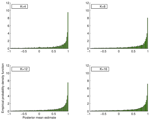
Figure 7: The empirical probability density functions of the posterior mean estimates with binary input conditioned on “+1” being transmitted.

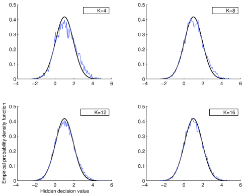
Figure 8: The empirical probability density functions of the “hidden” Gaussian statistic with binary input conditioned on “+1” being transmitted. The asymptotic Gaussian distribution predicted by the decoupling principle is also plotted for comparison.

In Figures 9–10, multiuser efficiency and spectral efficiency are plotted as functions of the average SNR. We consider three input distributions, namely, QPSK, 8PSK, and complex Gaussian inputs. Complex-valued spreading is assumed, where the multiuser efficiency and the spectral efficiency are given by Claim 5 and Corollary 3 respectively. We also consider two SNR distributions: 1) identical SNRs for all users (perfect power control), and 2) two groups of users of equal population with a power difference of 10 dB. We first assume a system load of $\beta=1$ and then redo the experiments with $\beta=3$.

In Figure 9, multiuser efficiency under complex Gaussian inputs and linear MMSE detection is plotted as a function of the average SNR. The load is $\beta=1$. We find the multiuser efficiencies decrease from 1 to 0 as the SNR increases. The monotonicity can be easily verified by inspecting the Tse-Hanly equation (54). Transmission with unbalanced power improves the multiuser efficiency. The corresponding spectral efficiencies of the system are plotted in Figure 9. Both joint decoding and separate decoding are considered. The gain in the spectral efficiency due to joint decoding is small for low SNR but significant for high SNR. Unbalanced SNR reduces the spectral efficiency, where under separate decoding the loss is almost negligible.

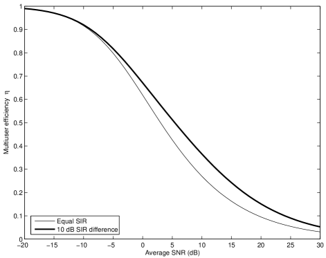
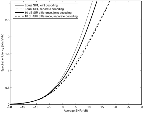
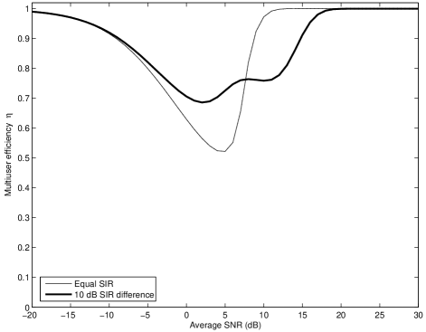
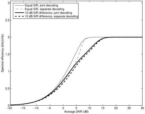
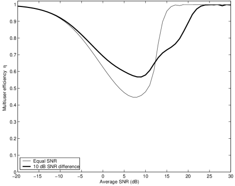
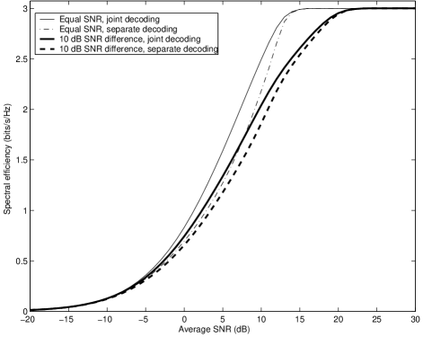
Figure 9: Multiuser efficiency and spectral efficiency as functions of SNR. The load is $\beta=1$. (a) Multiuser efficiency, complex Gaussian inputs. (b) Spectral efficiency, complex Gaussian inputs. (c) Multiuser efficiency, QPSK inputs. (d) Spectral efficiency, QPSK inputs. (e) Multiuser efficiency, 8PSK inputs. (f) Spectral efficiency, 8PSK inputs.

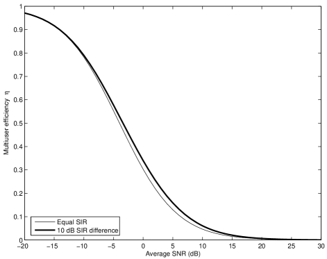
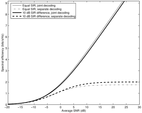
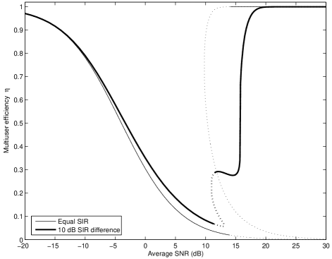
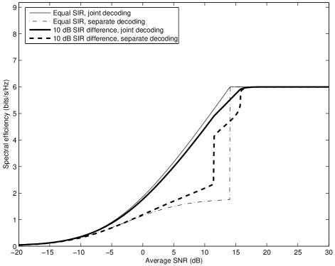
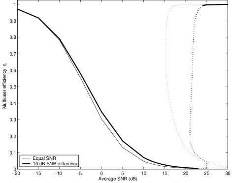
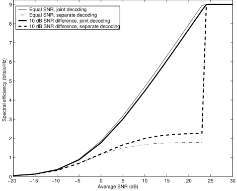
Figure 10: Multiuser efficiency and spectral efficiency as functions of SNR. The load is $\beta=3$. (a) Multiuser efficiency, complex Gaussian inputs. (b) Spectral efficiency, complex Gaussian inputs. (c) Multiuser efficiency, QPSK inputs. (d) Spectral efficiency, QPSK inputs. (e) Multiuser efficiency, 8PSK inputs. (f) Spectral efficiency, 8PSK inputs.

Multiuser efficiency with QPSK inputs and nonlinear MMSE (individually optimal) detection is plotted in Figure 9. Note that this function is not monotonic: it converges to 1 for both vanishing SNR and infinite SNR. While for vanishing SNR this follows directly from the definition of multiuser efficiency, the convergence to unity as the SNR goes to infinity was shown in [66] for the case of binary inputs. A single dip is observed for the case of identical SNRs while two dips are observed in the case of two SNRs of equal population with 10 dB difference in SNR (the gap is about 10 dB). The corresponding spectral efficiencies are plotted in Figure 9. The spectral efficiencies saturate to 1 bit/s/dimension at high SNR. The difference between joint decoding and separate decoding is quite small for both very low and very high SNRs while it can be 30% at around 6 dB.

Multiuser efficiency under 8PSK inputs and nonlinear MMSE detection is plotted in Figure 9. The multiuser efficiency curve is slightly better than that for QPSK inputs. The corresponding spectral efficiencies are plotted in Figure 9. The spectral efficiencies saturate to 3 bit/s/dimension at hight SNR.

In Figure 10, we redo the previous experiments only with a different system load $\beta=3$. The results are to be compared with those in Figure 9.

For Gaussian inputs, the multiuser efficiency curves in Figure 10 take a similar shape as in Figure 9, but are significantly lower due to higher load. The corresponding spectral efficiencies are shown in Figure 10. It is clear that higher load results in higher spectrum usage under joint decoding. Separate decoding, however, is interference limited and the spectral efficiency saturates under high SNR (cf. [10, Figure 1]).

Figure 10 plots multiuser efficiency under QPSK inputs. All solutions to the fixed-point equation (34) of the multiuser efficiency are shown. Under equal SNR, multiple solutions coexist for an average SNR of 10 dB or higher. If two groups of users with 10 dB difference in SNR, multiple solutions are seen between 11 to 13 dB. The solution that minimizes the free energy is valid and is shown in solid lines, while invalid solutions are plotted using dotted lines. An almost 0 to 1 jump is observed under equal SNR and a much smaller jump is seen under unbalanced SNRs. This is known as phase transition. The asymptotics under equal SNR can be shown by taking the limit ${\mathsf{snr}}\rightarrow\infty$ in (62). Essentially, if ${\mathsf{\eta}}{\mathsf{snr}}\rightarrow\infty$, then ${\mathsf{\eta}}\rightarrow 1$; while if ${\mathsf{\eta}}{\mathsf{snr}}\rightarrow\tau$ where $\tau$ is the solution to

$$\tau\int\frac{1}{\sqrt{2\pi}}e^{-\frac{z^{2}}{2}}[1-\tanh(\tau-z\sqrt{\tau})]{\,{\text{d}}}z=\frac{1}{\beta},$$ (184)

then ${\mathsf{\eta}}\rightarrow 0$. If $\beta>2.085$, there exists a solution to (184) so that two solutions coexist for large SNR.

The spectral efficiency under QPSK inputs and $\beta=3$ is shown in Figure 10. As a result of phase transition, one observes a jump to saturation in the spectral efficiency under equal-power inputs. The gain due to joint decoding can be significant in moderate SNRs. In case of two groups of users with 10 dB difference in SNR, the spectral efficiency curve also shows one jump and the loss due to separate decoding is reduced significantly for a small window of SNRs around the areas of phase transition (11–13 dB). Therefore, perfect power control may not be the best strategy in such cases.

Under 8PSK inputs, the multiuser efficiency and spectral efficiency curves in Figure 10 and 10 take similar shape as the curves under QPSK inputs. Phase transition causes jumps in both the multiuser efficiency and the spectral efficiency.

In Figures 10 and 10 a sharp bend upward is observed at the point of phase transition. This is known as “spinodal” in statistical physics.

A comparison of Figures 10, 10 and 10 shows that under separate decoding, the spectral efficiency under Gaussian inputs saturates well below that of QPSK and 8PSK inputs.

VII Conclusion

The main contribution of this paper is a simple characterization of the performance of CDMA multiuser detection under arbitrary input distribution and SNR (and/or flat fading) in the large-system limit. A broad family of multiuser detectors is studied under the name of posterior mean estimators, which includes well-known detectors such as the matched filter, decorrelator, linear MMSE detector, maximum likelihood (jointly optimal) detector, and the individually optimal detector.

A key conclusion is the decoupling of a Gaussian multiuser channel concatenated with a generic multiuser detector front end. It is found that the multiuser detection output for each user is a deterministic function of a hidden Gaussian statistic centered at the transmitted symbol. Hence the single-user channel seen at the multiuser detection output is equivalent to a Gaussian channel in which the overall effect of multiple-access interference is a degradation in the effective signal-to-interference ratio. The degradation factor, known as the multiuser efficiency, is the solution to a pair of coupled fixed-point equations, and can be easily computed numerically if not analytically.

Another set of results, tightly related to the decoupling principle, lead to general formulas for the large-system spectral efficiency of multiuser channels expressed in terms of the multiuser efficiency, both under joint and separate decoding. It is found that the decomposition of optimum spectral efficiency as a sum of single-user efficiencies and a joint decoding gain applies under more general conditions than shown in [11], thereby validating Müller’s conjecture [25]. A relationship between the spectral efficiencies under joint and separate decoding is one of the applications of a recent basic formula that links the mutual information and the MMSE [41].

From a practical viewpoint, this paper presents new results on the efficiency of CDMA communication under arbitrary input signaling such as $m$-PSK and $m$-QAM with an arbitrary power profile. More importantly, the results in this paper allow the performance of multiuser detection to be characterized by a single parameter, the multiuser efficiency. The efficiency of spectrum usage is also easily quantified by means of this parameter. Thus, the results offer convenient performance measures and valuable insights in the design and analysis of CDMA systems, e.g., in power control [67].

The linear system in our study also models multiple-input multiple-output channels under various circumstances. The results can thus be used to evaluate the output SNR or spectral efficiency of high-dimensional MIMO channels (such as multiple-antenna systems) with arbitrary signaling and various detection techniques. Some of the results in this paper have been generalized to MIMO channels with spatial correlation at both transmitter and receiver sides [68].

VIII Acknowledgements

The authors are grateful to the anonymous referees for their helpful reviews. Thanks also to Ralf Müller, Toshiyuki Tanaka and Chih-Chun Wang for interesting discussions.

References

- [1] S. Verdú, Multiuser Detection. Cambridge University Press, 1998.
- [2] S. Verdú, “Minimum probability of error for asynchronous multiple access communication systems,” in Proc. IEEE Military Communications Conference, vol. 1, Nov. 1983, pp. 213–219.
- [3] ——, “Optimum multiuser signal detection,” Ph.D. dissertation, Dept. of Electrical Engineering, University of Illinois at Urbana-Champaign, 1984, technical Report T-151, Coordinated Science Laboratory.
- [4] S. Verdú, “Minimum probability of error for asynchronous Gaussian multiple-access channels,” IEEE Trans. Inform. Theory, vol. 32, pp. 85–96, Jan. 1986.
- [5] S. Verdú, “Optimum multiuser asymptotic efficiency,” IEEE Trans. Inform. Theory, vol. 34, pp. 890–897, Sept. 1986.
- [6] D. N. C. Tse and S. V. Hanly, “Linear multiuser receivers: Effective interference, effective bandwidth and user capacity,” IEEE Trans. Inform. Theory, vol. 45, pp. 641–657, Mar. 1999.
- [7] Y. C. Eldar and A. M. Chan, “On the asymptotic performance of the decorrelator,” IEEE Trans. Inform. Theory, vol. 49, pp. 2309–2313, Sept. 2003.
- [8] D. Guo and S. Verdú, “Multiuser detection and statistical mechanics,” in Communications, Information and Network Security, V. Bhargava, H. V. Poor, V. Tarokh, and S. Yoon, Eds. Kluwer Academic Publishers, 2002, ch. 13, pp. 229–277.
- [9] D. Guo, S. Verdú, and L. K. Rasmussen, “Asymptotic normality of linear multiuser receiver outputs,” IEEE Trans. Inform. Theory, vol. 48, pp. 3080–3095, Dec. 2002.
- [10] S. Verdú and S. Shamai, “Spectral efficiency of CDMA with random spreading,” IEEE Trans. Inform. Theory, vol. 45, pp. 622–640, Mar. 1999.
- [11] S. Shamai and S. Verdú, “The impact of frequency-flat fading on the spectral efficiency of CDMA,” IEEE Trans. Inform. Theory, vol. 47, pp. 1302–1327, May 2001.
- [12] A. M. Tulino and S. Verdú, “Random matrix theory and wireless communications,” Foundations and Trends in Communications and Information Theory, vol. 1, pp. 1–182, 2004.
- [13] Z. D. Bai, “Methodologies in spectral analysis of large dimensional random matrices, a review,” Statistica Sinica, vol. 9, pp. 611–677, July 1999.
- [14] S. Verdú, “Capacity region of Gaussian CDMA channels: The symbol-synchronous case,” in Proc. 24th Allerton Conf. Commun., Control and Computing, Oct. 1986, pp. 1025–1034.
- [15] A. J. Grant and P. D. Alexander, “Random sequence multisets for synchronous code-division multiple-access channels,” IEEE Trans. Inform. Theory, vol. 44, pp. 2832–2836, Nov. 1998.
- [16] P. B. Rapajic and D. Popescu, “Information capacity of a random signature multiple-input multiple-output channel,” IEEE Trans. Commun., vol. 48, pp. 1245–1248, Aug. 2000.
- [17] G. J. Foschini, “Layered space-time architecture for wireless communication in a fading environment when using multiple antennas,” Bell Labs Technical Journal, vol. 1, pp. 41–59, 1996.
- [18] I. E. Telatar, “Capacity of multi-antenna Gaussian channels,” European Transactions on Telecommunications, vol. 10, pp. 585–595, Nov./Dec. 1999.
- [19] G. J. Rodgers, “Comment: Spectral analysis of random matrices using the replica method,” Statistica Sinica, vol. 9, pp. 662–667, 1999.
- [20] T. Tanaka, “Analysis of bit error probability of direct-sequence CDMA multiuser demodulators,” in Advances in Neural Information Processing Systems, T. K. Leen et al., Ed. The MIT Press, 2001, vol. 13, pp. 315–321.
- [21] ——, “Average-case analysis of multiuser detectors,” in Proceedings IEEE International Symposium on Information Theory. Washington, D.C., June 2001, p. 287.
- [22] ——, “Statistical mechanics of CDMA multiuser demodulation,” Europhysics Letters, vol. 54, pp. 540–546, 2001.
- [23] ——, “A statistical mechanics approach to large-system analysis of CDMA multiuser detectors,” IEEE Trans. Inform. Theory, vol. 48, pp. 2888–2910, Nov. 2002.
- [24] R. R. Müller and W. H. Gerstacker, “On the capacity loss due to separation of detection and decoding,” IEEE Trans. Inform. Theory, vol. 50, pp. 1769–1778, Aug. 2004.
- [25] R. R. Müller, “On channel capacity, uncoded error probability, ML-detection and spin glasses,” in Proc. Workshop on Concepts in Information Theory. Breisach, Germany, 2002, pp. 79–81.
- [26] S. F. Edwards and P. W. Anderson, “Theory of spin glasses,” Journal of Physics F: Metal Physics, vol. 5, pp. 965–974, 1975.
- [27] H. Nishimori, Statistical Physics of Spin Glasses and Information Processing: An Introduction, ser. Number 111 in International Series of Monographs on Physics. Oxford University Press, 2001.
- [28] N. Sourlas, “Spin-glass models as error-correcting codes,” Nature, vol. 339, pp. 693–695, June 1989.
- [29] Y. Kabashima and D. Saad, “Statistical mechanics of error-correcting codes,” Europhysics Letters, vol. 45, pp. 97–103, 1999.
- [30] A. Montanari, “Turbo codes: The phase transition,” European Physical Journal B, vol. 18, pp. 121–136, 2000.
- [31] T. Murayama, Y. Kabashima, D. Saad, and R. Vicente, “Statistical physics of regular low-density parity-check error-correcting codes,” Physical Review E, vol. 62, pp. 1577–1591, 2000.
- [32] A. Montanari and N. Sourlas, “The statistical mechanics of turbo codes,” European Physical Journal B, vol. 18, pp. 107–119, 2000.
- [33] Y. Kabashima and D. Saad, “Statistical mechanics of low-density parity-check codes,” Journal of Physics A: Mathematical and General, vol. 37, pp. R1–R43, 2004.
- [34] A. L. Moustakas, S. H. Simon, and A. M. Sengupta, “MIMO capacity through correlated channels in the presence of correlated interferers and noise: A (not so) large analysis,” IEEE Trans. Inform. Theory, vol. 49, pp. 2545–2561, Oct. 2003.
- [35] Y. Kabashima, “A CDMA multiuser detection algorithm on the basis of belief propagation,” Journal of Physics A: Mathematical and General, vol. 36, pp. 11 111–11 121, 2003.
- [36] T. Fabricius and O. Winther, “Correcting the bias of subtractive interference cancellation in CDMA: Advanced mean field theory,” IEEE Trans. Inform. Theory, 2003, submitted.
- [37] M. Talagrand, “Rigorous results for mean field models for spin glasses,” Theoretical Computer Science, vol. 265, pp. 69–77, Aug. 2001.
- [38] ——, Spin Glasses: A Challenge for Mathematicians. Springer, 2003.
- [39] M. Mezard, G. Parisi, and M. A. Virasoro, Spin Glass Theory and Beyond. World Scientific, 1987.
- [40] V. Dotsenko, The Theory of Spin Glasses and Neural Networks. World Scientific, 1994.
- [41] D. Guo, S. Shamai, and S. Verdú, “Mutual information and minimum mean-square error in Gaussian channels,” IEEE Trans. Inform. Theory, Apr. 2005, to appear.
- [42] M. K. Varanasi and T. Guess, “Optimum decision feedback multiuser equalization with successive decoding achieves the total capacity of the Gaussian multiple-access channel,” in Proc. Asilomar Conf. on Signals, Systems and Computers. Monterey, CA, USA, Nov. 1997, pp. 1405–1409.
- [43] P. Rapajic, M. Honig, and G. Woodward, “Multiuser decision-feedback detection: Performance bounds and adaptive algorithms,” in Proceedings IEEE International Symposium on Information Theory. Cambridge, MA USA, Aug. 1998, p. 34.
- [44] S. L. Ariyavisitakul, “Turbo space-time processing to improve wireless channel capacity,” IEEE Trans. Commun., vol. 48, pp. 1347–1359, Aug. 2000.
- [45] R. R. Müller, “Multiuser receivers for randomly spread signals: Fundamental limits with and without decision-feedback,” IEEE Trans. Inform. Theory, vol. 47, pp. 268–283, Jan. 2001.
- [46] T. Guess and M. K. Varanasi, “An information-theoretic framework for deriving canonical decision-feedback receivers in Gaussian channels,” IEEE Trans. Inform. Theory, vol. 51, pp. 173–187, Jan. 2005.
- [47] G. D. Forney, Jr., “Shannon meets Wiener II: On MMSE estimation in successive decoding schemes,” in Proc. 42nd Allerton Conf. Commun., Control, and Computing. Monticello, IL, USA, 2004. [Online]. Available: http://arxiv.org/pdf/cs.IT/0409011
- [48] F. Comets, “The martingale method for mean-field disordered systems at high temperature,” in Mathematical Aspects of Spin Glasses and Neural Networks, A. Bovier and P. Picco, Eds. Birkhäuser, 1998, pp. 91–113.
- [49] T. M. Cover and J. A. Thomas, Elements of Information Theory. Wiley, 1991.
- [50] J. Yedidia, W. Freeman, and Y. Weiss, “Generalized belief propagation,” in Advances in Neural Information Processing Systems 13. MIT Press, 2001, pp. 689–695.
- [51] P. Pakzad and V. Anantharam, “Belief propagation and statistical physics,” in Proc. Conf. Inform. Sci. Sys. Princeton, NJ, USA, Mar. 2002.
- [52] J. van Mourik, D. Saad, and Y. Kabashima, “Critical noise levels for LPDC decoding,” Physics Review E, vol. 66, pp. 026 705:1–8, 2002.
- [53] M. Chiang and S. Boyd, “Geometric programming duals of channel capacity and rate distortion,” IEEE Trans. Inform. Theory, vol. 50, pp. 245–258, Feb. 2004.
- [54] R. R. Müller, “Random matrices, free probability, and the replica method,” in Proceedings of European Signal Processing Conference, Vienna, Austria, 2004.
- [55] D. Guo and S. Verdú, “Minimum probability of error of many-user CDMA without power control,” in Proceedings 2002 IEEE International Symposium on Information Theory. Lausanne, Switzerland, 2002, p. 188.
- [56] ——, “Replica analysis of CDMA spectral efficiency,” in Proceedings 2003 IEEE Information Theory Workshop. Paris, France, 2003.
- [57] D. Guo, “Gaussian channels: Information, estimation and multiuser detection,” Ph.D. dissertation, Department of Electrical Engineering, Princeton University, 2004.
- [58] R. R. Müller, “Channel capacity and minimum probability of error in large dual antenna array systems with binary modulation,” IEEE Trans. Signal Processing, vol. 51, pp. 2821–2828, Nov. 2003.
- [59] G. Caire, “Statistical physics and the analysis of exact belief-propagation decoding of CDMA,” in Proc. JWCC. Barolo, Italy, 2002, pp. 30–32.
- [60] G. Caire, R. R. Müller, and T. Tanaka, “Iterative multiuser joint decoding: Optimal power allocation and low-complexity implementation,” IEEE Trans. Inform. Theory, vol. 50, pp. 1950–1973, Sept. 2004.
- [61] T. Tanaka and M. Okada, “Approximate belief propagation, density evolution, and statistical neurodynamics for CDMA multiuser detection,” IEEE Trans. Inform. Theory, vol. 51, pp. 700–706, Feb. 2005.
- [62] R. S. Ellis, Entropy, Large Deviations, and Statistical Mechanics, ser. A series of comprehensive studies in mathematics. Springer-Verlag, 1985, vol. 271.
- [63] H. Nishimori and D. Sherrington, “Absence of replica symmetry breaking in a region of the phase diagram of the Ising spin glass,” in AIP Conf. Proc. 553: Disordered and Complex Systems, 2001, p. 67.
- [64] J. Hubbard, “Calculation of partition functions,” Physics Review Letters, vol. 3, pp. 77–78, 1959.
- [65] W. Feller, An Introduction to Probability Theory and Its Applications, 2nd ed. John Wiley & Sons, Inc., 1971, vol. II.
- [66] D. N. C. Tse and S. Verdú, “Optimum asymptotic multiuser efficiency for randomly spread CDMA,” IEEE Trans. Inform. Theory, vol. 46, pp. 2718–2722, Nov. 2000.
- [67] F. Meshkati, D. Guo, H. V. Poor, S. Schwartz, and N. B. Mandayam, “A unified approach to power control for multiuser detectors,” in Proceedings 2nd International Workshop on Signal Processing for Wireless Communications. London, England, 2004.
- [68] C.-K. Wen and K.-K. Wong, “Asymptotic spectral efficiency of spatially correlated MIMO multiple-access channels with arbitrary signaling inputs for joint and separate decoding,” in Proceedings IEEE International Symposium on Information Theory. Chicago, IL, USA, 2004, p. 282.