Hiding Satisfying Assignments: Two are Better than One

Abstract

The evaluation of incomplete satisfiability solvers depends critically on the availability of hard satisfiable instances. A plausible source of such instances consists of random $k$-SAT formulas whose clauses are chosen uniformly from among all clauses satisfying some randomly chosen truth assignment $A$. Unfortunately, instances generated in this manner tend to be relatively easy and can be solved efficiently by practical heuristics. Roughly speaking, as the formula’s density increases, for a number of different algorithms, $A$ acts as a stronger and stronger attractor. Motivated by recent results on the geometry of the space of satisfying truth assignments of random $k$-SAT and NAE-$k$-SAT formulas, we introduce a simple twist on this basic model, which appears to dramatically increase its hardness. Namely, in addition to forbidding the clauses violated by the hidden assignment $A$, we also forbid the clauses violated by its complement, so that both $A$ and $\overline{A}$ are satisfying. It appears that under this “symmetrization” the effects of the two attractors largely cancel out, making it much harder for algorithms to find any truth assignment. We give theoretical and experimental evidence supporting this assertion.

1 Introduction

Recent years have witnessed the rapid development and application of search methods for constraint satisfaction and Boolean satisfiability. An important factor in the success of these algorithms is the availability of good sets of benchmark problems to evaluate and fine-tune them. There are two main sources of such problems: the real world, and random instance generators. Real-world problems are arguably the best benchmark, but unfortunately are often in short supply. Moreover, using real-world problems carries the risk of tuning algorithms toward the specific application domains for which good benchmarks are available. In that sense, random instance generators are a good additional source, with the advantage of controllable characteristics, such as size and expected hardness.

Hard random instances have led to the development of new stochastic search methods such as WalkSAT [28] and the breakout procedure [26], and have been used in detailed comparisons of local search methods for graph coloring and related graph problems [17]. The results of various competitions for CSP and SAT algorithms show a fairly direct correlation between the performance on real-world benchmarks and on hard random instances [16, 13, 17]. Nevertheless, a key limitation of current problem generators concerns their use in evaluating incomplete satisfiability solvers such as those based on local search methods.

When an incomplete algorithm does not find a solution, it can be difficult to determine whether this is because the instance is in fact unsatisfiable, or simply because the algorithm failed to find the satisfying assignment. The standard way of dealing with this problem is to use a complete search method to filter out the unsatisfiable cases. However, this greatly limits the size and difficulty of problem instances that can be considered. Ideally, one would use problem generators that generate satisfiable instances only. One relatively recent source of such problems is the quasigroup completion problem [29, 3, 19]. However, a generator for random hard satisfiable instances of 3-SAT, say, has remained elusive.

Perhaps the most natural candidate for generating random hard satisfiable 3-SAT formulas is the following. Pick a random truth assignment $A$, and then generate a formula with $n$ variables and $rn$ random clauses, rejecting any clause that is violated by $A$. In particular, we might hope that if we work close to the satisfiability threshold region $r\approx 4.25$, where the hardest random 3-SAT problems seem to be [10, 15, 25], this would generate hard satisfiable instances. Unfortunately, this generator is highly biased towards formulas with many assignments clustered around $A$. When given to local search methods such as WalkSAT, the resulting formulas turn out to be much easier than formulas of comparable size obtained by filtering satisfiable instances from a 3-SAT generator. More sophisticated versions of this “hidden assignment” scheme [7, 30] improve matters somewhat but still lead to easily solvable formulas.

In this paper we introduce a new generator of random satisfiable problems. The idea is simple: we pick a random 3-SAT formula that has a “hidden” complementary pair of satisfying assignments, $A$ and $\overline{A}$, by rejecting clauses that are violated by either $A$ or $\overline{A}$. We call these “2-hidden” formulas. Our motivation comes from recent work [4, 6] which showed that moving from random $k$-SAT to random NAE-$k$-SAT (in which every clause in the formula must have at least one true and at least one false literal) tremendously reduces the correlation between solutions. That is, whereas in random $k$-SAT, satisfying assignments tend to form clumps, in random NAE-$k$-SAT the solutions appear to be scattered throughout $\{0,1\}^{n}$ in a rather uniform “mist”, even for densities extremely close to the threshold. An intuitive explanation for this phenomenon is that since the complement of every NAE-assignment is also an NAE-assignment, the attractions of solution pairs largely “cancel out.” In this paper we exploit this phenomenon to impose a similar symmetry on the hidden assignments $A$ and $\overline{A}$, so that their attractions cancel out, making it hard for a wide variety of algorithms to “feel” either one.

A particularly nice feature of our generator is that it is based on an extremely simple probabilistic procedure, in sharp contrast with 3-SAT generators based on, say, cryptographic ideas [23]. In particular, our generator is readily amenable to all the mathematical tools that have been developed for the rigorous study of random $k$-SAT formulas. Here we make two first steps in that direction. In Section 2, via a first moment calculation we study the distribution of the number of solutions as a function of their distance from the hidden assignments. In Section 3, on the other hand, we use the technique of differential equations to analyze the performance of the Unit Clause (UC) heuristic on our formulas.

Naturally, mathematical simplicity would not be worth much if the formulas produced by our generator were easily solvable. In Section 4, we compare experimentally the hardness of “2-hidden” formulas with that of “1-hidden” and “0-hidden” formulas. That is, we compare our formulas with random 3-SAT formulas with one hidden assignment and with standard random 3-SAT formulas with no hidden assignment. We examine four leading algorithms: two complete solvers, zChaff and Satz, and two incomplete ones, WalkSAT and the recently introduced Survey Propagation (SP).

For all these algorithms, we find that our formulas are much harder than 1-hidden formulas and, more importantly, about as hard as 0-hidden formulas, of the same size and density.

2 A picture of the space of solutions

In this section we compare 1-hidden and 2-hidden formulas with respect to the expected number of solutions at a given distance from the hidden assignment(s).

2.1 1-hidden formulas

Let $X$ be the number of satisfying truth assignments in a random $k$-SAT formula with $n$ variables and $m=rn$ clauses chosen uniformly and independently among all $k$-clauses with at least one positive literal, i.e., 1-hidden formulas where we hide the all–ones truth assignment. To calculate the expectation ${\bf E}[X]$, it is helpful to parametrize truth assignments according to their overlap with the hidden assignment, i.e., the fraction $\alpha$ of variables on which they agree with $A$, which in this case is the fraction of variables that are set to one. Then, linearity of expectation gives (1), clause independence gives (2), selecting the literals in each clause uniformly and independently gives (2.1), and, finally, writing $z=\alpha n$ and using Stirling’s approximation for the factorial gives (2.1):

$${\bf E}[X] = \sum_{A\in\{0,1\}^{n}}\Pr[A\mbox{ is satisfying}]$$ (1)

$$= \sum_{z=0}^{n}\binom{n}{z}\Pr[\mbox{a truth assignment with $z$ ones satisfies a random clause}]^{m}$$ (2)

$$= \sum_{z=0}^{n}\binom{n}{z}\left(1-\frac{1}{2^{k}-1}\sum_{j=1}^{k}\binom{k}{j}(1-z/n)^{j}(z/n)^{k-j}\right)^{m}$$

$$= \sum_{z=0}^{n}\binom{n}{z}\left(1-\frac{1-(z/n)^{k}}{2^{k}-1}\right)^{m}$$

$$= {\mathrm{poly}}(n)\times\max_{\alpha\in[0,1]}\left[\frac{1}{\alpha^{\alpha}(1-\alpha)^{1-\alpha}}\left(1-\frac{1-\alpha^{k}}{2^{k}-1}\right)^{r}\right]^{n}$$

$$\equiv {\mathrm{poly}}(n)\times\max_{\alpha\in[0,1]}[f_{k,r}(\alpha)]^{n^{\phantom{k^{k^{k}}}}}$$

where

$$f_{k,r}(\alpha)=\frac{1}{\alpha^{\alpha}(1-\alpha)^{1-\alpha}}\left(1-\frac{1-\alpha^{k}}{2^{k}-1}\right)^{r}\enspace.$$

From this calculation we see that ${\bf E}[X]$ is dominated by the contribution of the truth assignments that maximize $f_{k,r}(\alpha)$ (since we raise $f_{k,r}$ to the $n$th power all other contributions vanish). Now, we readily see that $f$ is the product of an “entropic” factor $1/(\alpha^{\alpha}(1-\alpha)^{1-\alpha})$ which is symmetric around $\alpha=1/2$, and a “correlation” factor which is strictly increasing in $\alpha$. As a result, it is always maximized for some $\alpha>1/2$. This means that the dominant contribution to ${\bf E}[X]$ comes from truth assignments that agree with the hidden assignment on more that half the variables. That is, the set of solutions is dominated by truth assignments that can “feel” the hidden assignments. Moreover, as $r$ increases this phenomenon becomes more and more acute (see Figure 1 below).

2.2 2-hidden formulas

Now let $X$ be the number of satisfying truth assignments in a random $k$-SAT formula with $n$ variables and $m=rn$ clauses chosen uniformly among all $k$-clauses that have at least one positive and at least one negative literal, i.e., 2-hidden formulas where we hide the all–ones assignment and its complement. To compute ${\bf E}[X]$ we proceed as above, except that now (2.1) is replaced by

$$\sum_{z=0}^{n}\binom{n}{z}\left(1-\frac{1}{2^{k}-2}\sum_{j=1}^{k-1}\binom{k}{j}(1-z/n)^{j}(z/n)^{k-j}\right)^{m}\enspace.$$

Carrying through the ensuing changes we find that now

$${\bf E}[X]={\mathrm{poly}}(n)\times\max_{\alpha\in[0,1]}[g_{k,r}(\alpha)]^{n}$$

where

$$g_{k,r}(\alpha)=\frac{1}{\alpha^{\alpha}(1-\alpha)^{1-\alpha}}\left(1-\frac{1-\alpha^{k}-(1-\alpha)^{k}}{2^{k}-2}\right)^{r}\enspace.$$

This time, both the entropic factor and the correlation factor comprising $g$ are symmetric functions of $\alpha$, so $g_{k,r}$ is symmetric around $\alpha=1/2$ (unlike $f_{k,r}$). Indeed, one can prove that for all $r$ up to extremely close to the random $k$-SAT threshold $r_{k}$, the function $g_{k,r}$ has its global maximum at $\alpha=1/2$. In other words, for all such $r$, the dominant contribution to ${\bf E}[X]$ comes from truth assignments at distance $n/2$ from the hidden assignments, i.e., the hidden assignments are “not felt.” More precisely, there exists a sequence $\epsilon_{k}\rightarrow 0$ such that $g_{k,r}$ has a unique global maximum at $\alpha=1/2$, for all

$$r\leq 2^{k}\ln 2-\frac{\ln 2}{2}-1-\epsilon_{k}\enspace.$$ (5)

Contrast this with the fact (implicit in [20]) that for

$$r\geq 2^{k}\ln 2-\frac{\ln 2}{2}-\frac{1}{2}\enspace,$$ (6)

a random $k$-SAT formula with $n$ variables and $m=rn$ clauses is unsatisfiable with probability $1-o(1)$. Moreover, the convergence of the sequence $\epsilon_{k}\to 0$ is rapid, as can be seen from the concrete values in table 1.

$$\begin{array}[]{l|cccccc}\hskip 2.84544ptk&\makebox[34.14322pt]{3}&\makebox[36.98866pt]{4}&\makebox[39.83368pt]{5}&\makebox[42.67912pt]{7}&\makebox[45.52458pt]{10}&\makebox[48.36958pt]{20}\\ \hline\cr\mbox{Eq.\ \eqref{lower}}&7/2&35/4&20.38&87.23&708.40&726816.15\\ \mbox{Eq.\ \eqref{upper}}&4.67&10.23&21.33&87.88&708.94&726816.66\end{array}$$

Table 1: The convergence (in $k$) to the asymptotic gap of $1/2$ is rapid

Below we plot $f_{k,r}$ and $g_{k,r}$ for $k=5$ and $r=16,18,20,22,24$ (from top to bottom). We see that in the case of 1-hidden formulas, i.e., $f_{k,r}$, the maximum always occurs to the right of $\alpha=1/2$. Moreover, observe that for $r=22,24$, i.e., after we cross the 5-SAT threshold (which occurs at $r\approx 21$) we have a dramatic shift in the location of the maximum and, thus, in the extent of the bias: as one would expect, the only remaining satisfying assignments above the threshold are those extremely close to the hidden assignment.

In the case of 2-hidden formulas, on the other hand, we see that for $r=16,18,20$ the global maximum occurs at $\alpha=1/2$ (from the table above we know that the critical $r$ for $k=5$ is $20.38$). For $r=20$, we also have two local maxima, near $\alpha=0,1$, but since $g_{k,r}$ is raised to the $n$th power, these are exponentially suppressed. Naturally, for $r$ above the threshold, i.e., $r=22,24$, these local maxima become global, signifying that indeed the only remaining truth assignments are those extremely close to one of the two hidden ones.

Intuitively, we expect that because $g$ is flat at $\alpha=1/2$ where random truth assignments are concentrated, for 2-hidden formulas local search algorithms like WalkSAT will essentially perform a random walk until they are lucky enough to get close to one of the two hidden assignments. Thus we expect WalkSAT to take about as long on 2-hidden formulas as it does on 0-hidden ones. For 1-hidden formulas, in contrast, we expect the nonzero gradient of $f$ at $\alpha=1/2$ to provide a strong “hint” to WalkSAT that it should move towards the hidden assignment, and that therefore 1-hidden formulas will be much easier for it to solve. We will see below that our experimental results bear out these intuitions perfectly.

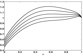
1-hidden formulas

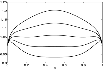
2-hidden formulas

Figure 1: The $n$th root of the expected number of solutions $f_{k,r}$ and $g_{k,r}$ for 1-hidden and 2-hidden formulas respectively, as a function of the overlap fraction $\alpha=z/n$ with the hidden assignment. Here $k=5$ and $r=16,18,20,22,24$ from top to bottom.

3 The Unit Clause heuristic and DPLL algorithms

Consider the following linear-time heuristic, called Unit Clause (UC), which permanently sets one variable in each step as follows: pick a random literal and satisfy it; repeatedly satisfy any 1-clauses present. In [9], Chao and Franco showed that UC succeeds with constant probability on random 3-SAT formulas with $r<8/3$, and fails with high probability, i.e., with probability $1-o(1)$ as $n\to\infty$, for $r>8/3$. One can think of UC as the first branch of the simplest possible DPLL algorithm $S$: set variables in a random order, each time choosing randomly which branch to take first. The result of [9] then shows that, with constant probability, $S$ solves random 3-SAT formulas with $r<8/3$ with no backtracking at all.

Conversely, calculations from statistical physics [11, 12] suggest that with high probability $S$ takes exponential time for all $r>8/3$. That is, around $r=8/3$ the running time of $S$ goes from linear to exponential, with no intermediate regime. In [2], it was proved that $S$ takes exponential time for $r>3.81$, which is already well below the conjectured satisfiability threshold $r\approx 4.2$. Moreover, the results in [2] imply that if the “tricritical point” of $(2+p)$-SAT is $r=2/5$, one can replace 3.81 with 8/3.

In this section we analyze the performance of UC on 1-hidden and 2-hidden formulas. Specifically, we show that UC fails for 2-hidden formulas at precisely the same density as for 0-hidden ones. Based on this, we conjecture that the running time of $S$, and other simple DPLL algorithms, becomes exponential for 2-hidden formulas at the same density as for 0-hidden ones.

To analyze UC on random 1-hidden and 2-hidden formulas we actually analyze UC on arbitrary initial distributions of 3-clauses, i.e., where for each $0\leq j\leq 3$ we specify the initial number of 3-clauses with $j$ positive literals and $3-j$ negative ones. We use the method of differential equations; see [1] for a review. To simplify notation, we assume that $A$ is the all–ones assignment, so that 1-hidden formulas forbid clauses where all literals are negative, while 2-hidden formulas forbid all-negative and all-positive clauses.

A round of UC consists of a free step, in which we satisfy a random literal, and the ensuing chain of unit-clause propagations. For $0\leq i\leq 3$ and $0\leq j\leq i$, let $S_{i,j}=s_{i,j}n$ be the number of clauses of length $i$ with $j$ positive literals and $i-j$ negative ones. We will also refer to the total density of clauses of size $i$ as $s_{i}=\sum_{j}s_{i,j}$. Let $X=xn$ be the number of variables set so far. Our goal is to write the expected change in these variables in a given round as a function of their values at the beginning of the round. Note that at the beginning of each round $S_{1,0}=S_{1,1}=0$ by definition, so the “state space” of our analysis will consist of the variables $S_{i,j}$ for $i\geq 2$.

It is convenient to define two new quantities, $m_{T}$ and $m_{F}$, which are the expected number of variables set True and False in a round. We will calculate these below. Then, in terms of $m_{T},m_{F}$, we have

$${\bf E}[\Delta S_{3,j}] = -(m_{T}+m_{F})\,\frac{3s_{3,j}}{1-x}$$ (7)

$${\bf E}[\Delta S_{2,j}] = -(m_{T}+m_{F})\,\frac{2s_{2,j}}{1-x}+m_{F}\,\frac{(j+1)s_{3,j+1}}{1-x}+m_{T}\,\frac{(3-j)s_{3,j}}{1-x}$$ (8)

$${\bf E}[\Delta X] = -(m_{T}+m_{F})\enspace.$$

To see this, note that a variable appears positively in a clause of type $i,j$ with probability $j/(n-X)$, and negatively with probability $(i-j)/(n-X)$. Thus, the negative terms in (7) and (8) correspond to clauses being “hit” by the variables set, while the positive term is the “flow” of 3-clauses to 2-clauses.

To calculate $m_{T}$ and $m_{F}$, we consider the process by which unit clauses are created during a round. We can model this with a two-type branching process, which we analyze as in [5]. Since the free step gives the chosen variable a random value, we can think of it as creating a unit clause, which is positive or negative with equal probability. Thus the initial expected population of unit clauses can be represented by a vector

$$p_{0}=\left(\begin{array}[]{c}1/2\\ 1/2\end{array}\right)$$

where the first and second components count the negative and positive unit clauses respectively. Moreover, at time $X=xn$, a unit clause procreates according to the matrix

$$M=\frac{1}{1-x}\left(\begin{array}[]{cc}s_{2,1}&2s_{2,0}\\ 2s_{2,2}&s_{2,1}\end{array}\right)\enspace.$$

In other words, satisfying a negative unit clause creates, in expectation, $M_{1,1}=s_{2,1}/(1-x)$ negative unit clauses and $M_{2,1}=2s_{2,2}/(1-x)$ positive unit clauses, and similarly for satisfying a positive unit clause.

Thus, as long as the largest eigenvalue $\lambda_{1}$ of $M$ is less than $1$, the expected number of variables set true or false during the round is given by

$$\left(\begin{array}[]{c}m_{F}\\ m_{T}\end{array}\right)=(I+M+M^{2}+\cdots)\cdot p_{0}=\left(I-M\right)^{-1}\cdot p_{0}$$

where $I$ is the identity matrix. Moreover, as long as $\lambda_{1}<1$ throughout the algorithm, i.e., as long as the branching process is subcritical for all $x$, UC succeeds with constant probability. On the other hand, if $\lambda_{1}$ ever exceeds $1$, then the branching process becomes supercritical, with high probability the unit clauses proliferate and the algorithm fails. Note that

$$\lambda_{1}=\frac{s_{2,1}+2\sqrt{s_{2,0}\,s_{2,2}}}{1-x}\enspace.$$ (9)

Now let us rescale (7) to give a system of differential equations for the $s_{i,j}$. Wormald’s Theorem [31] implies that w.h.p. the random variables $S_{i,j}(xn)$ will be within $o(n)$ of $s_{i,j}(x)\cdot n$ for all $x$:

$$\frac{{\rm d}s_{3,j}}{{\rm d}x} = -\frac{3s_{3,j}}{1-x}$$ (10)

$$\frac{{\rm d}s_{2,j}}{{\rm d}x} = -\frac{2s_{2,j}}{1-x}+\frac{m_{F}}{m_{T}+m_{F}}\,\frac{(j+1)s_{3,j+1}}{1-x}+\frac{m_{T}}{m_{T}+m_{F}}\,\frac{(3-j)s_{3,j}}{1-x}$$

Now, suppose our initial distribution of 3-clauses is symmetric, i.e., $s_{3,0}(0)=s_{3,3}(0)$ and $s_{3,1}(0)=s_{3,2}(0)$. It is easy to see from (10) that in that case, both the 3-clauses and the 2-clauses are symmetric at all times, i.e., $s_{i,j}=s_{i,i-j}$ and $m_{F}=m_{T}$. In that case $s_{2,1}+2\sqrt{s_{2,0}s_{2,2}}=s_{2}$, so the criterion for subcriticality becomes

$$\lambda_{1}=\frac{s_{2}}{1-x}<1\enspace.$$

Moreover, since the system (10) is now symmetric with respect to $j$, summing over $j$ gives the differential equations

$$\frac{{\rm d}s_{3}}{{\rm d}x} = -\frac{3s_{3}}{1-x}$$

$$\frac{{\rm d}s_{2}}{{\rm d}x} = -\frac{2s_{2}}{1-x}+\frac{3s_{3}}{2(1-x)}$$

which are precisely the differential equations for UC on 0-hidden formulas, i.e., random instances of 3-SAT.

Since 2-hidden formulas correspond to symmetric initial conditions, we have thus shown that UC succeeds on them with constant probability if and only if $r<8/3$, i.e., that UC fails on these formulas at exactly the same density for which it fails on random 3-SAT instances. (In contrast, integrating (10) with the initial conditions corresponding to 1-hidden formulas shows that UC succeeds for them at a slightly higher density, up to $r<2.679$.)

Of course, UC can easily be improved by making the free step more intelligent: for instance, choosing the variable according the number of its occurrences in the formula, and using the majority of these occurrences to decide its truth value. The best known heuristic of this type [18, 14] succeeds with constant probability for $r<3.52$. However, we believe that much of the progress that has been made in analyzing the performance of such algorithms can be “pushed through” to 2-hidden formulas. Specifically, nearly all algorithms analyzed so far have the property that given as input a symmetric initial distribution of 3-clauses, e.g. random 3-SAT, their residual formulas consist of symmetric mixes of 2- and 3-clauses. As a result, we conjecture that the above methods can be used to show that such algorithms act on 2-hidden formulas exactly as they do on 0-hidden ones, failing w.h.p. at the same density.

More generally, call a DPLL algorithm myopic if its splitting rule consists of choosing a random clause of a given size, based on the current distribution of clause sizes, and deciding how to satisfy it based on the number of occurrences of its variables in other clauses. For a given myopic algorithm $A$, let $r_{A}$ be the density below which $A$ succeeds without any backtracking with constant probability. The results of [2] imply the following statement: if the tricritical point for random $(2+p)$-SAT is $p_{c}=2/5$ then every myopic algorithm $A$ takes exponential time for $r>r_{A}$. Thus, not only UC, but in fact a very large class of natural DPLL algorithms, would go from linear time for $r<r_{A}$ to exponential time for $r>r_{A}$. The fact that the linear-time heuristics corresponding to the first branch of $A$ act on 2-hidden formulas just as they do on 0-hidden ones suggests that, for a wide variety of DPLL algorithms, 2-hidden formulas become exponentially hard at the same density as 0-hidden ones. Proving this, or indeed proving that 2-hidden formulas take exponential time for $r$ above some critical density, appears to us a very promising direction for future work.

4 Experimental results

In this section we report experimental results on our 2-hidden formulas, and compare them to 1-hidden and 0-hidden ones. We use two leading complete solvers, zChaff and Satz, and two leading incomplete solvers, WalkSAT and the new Survey Propagation algorithm SP. In an attempt to avoid the numerous spurious features present in “too-small” random instances, i.e., in non-asymptotic behavior, we restricted our attention to experiments where $n\geq 1000$. This meant that zChaff and Satz could only be examined at densities significantly above the satisfiability threshold, as neither algorithm could practically solve either 0-hidden or 2-hidden formulas with $n\sim 1000$ variables close to the threshold. For WalkSAT and SP, on the other hand, we can easily run experiments in the hardest range (around the satisfiability threshold) for $n\sim 10^{4}$.

4.1 zChaff and Satz

In order to do experiments with $n\geq 1000$ with zChaff and Satz, we focused on the regime where $r$ is relatively large, $20<r<60$. As stated above, for $r$ near the satisfiability threshold, 0-hidden and 2-hidden random formulas with $n\sim 1000$ variables seem completely out of the reach of either algorithm. While formulas in this overconstrained regime are still challenging, the presence of many forced steps allows both solvers to completely explore the space fairly quickly.

We obtained zChaff from the Princeton web site [27]. The left part of Figure 2 shows its performance on random formulas of all three types (with $n=1000$ for $20\leq r\leq 40$ and $n=3000$ for $40\leq n\leq 60$). We see that the number of decisions for all three types of problems decreases rapidly as $r$ increases, consistent with earlier findings for complete solvers on random 3-SAT formulas.

Figure 2 shows that zChaff finds 2-hidden formulas almost as difficult as 0-hidden ones, which for this range of $r$ are unsatisfiable with overwhelming probability. On the other hand, the 1-hidden formulas are much easier, with a number of branchings between 2 and 5 orders of magnitude smaller. It appears that while zChaff’s smarts allow it to quickly “zero in” on a single hidden assignment, the attractions exerted by a complementary pair of assignments do indeed cancel out, making 2-hidden formulas almost as hard as unsatisfiable ones. That is, the algorithm eventually “stumbles” upon one of the two hidden assignments after a search that is nearly as exhaustive as for the unsatisfiable random 3-SAT formulas of the same density.

We obtained Satz from the SATLIB web site [22]. The right part of Figure 2 shows experiments on random formulas of all three types with $n=3000$. As for zChaff, the 2-hidden formulas are almost as hard for Satz as the 0-hidden formulas are. On the other hand, the 1-hidden formulas are too. Indeed, Figure 2 shows that the median number of branches for all three types of formulas is within a multiplicative constant.

The reason for this is simple: while Satz makes intelligent decisions about which variable to branch on, it tries these branches in a fixed order, attempting first to set each variable false [21]. Therefore, a single hidden assignment will appear at a uniformly random leaf in Satz’s search tree. In the 2-hidden case, since the two hidden assignments are complementary, one will appear in a random position and the other one in the symmetric position with respect to the search tree. Naturally, trying branches in a fixed order is a good idea when the true goal is to prove that a formula is unsatisfiable, e.g. in hardware verification. However, we expect that if Satz were modified to, say, use the majority heuristic to choose a variable’s first value, its performance on the three types of problems would be similar to zChaff’s.

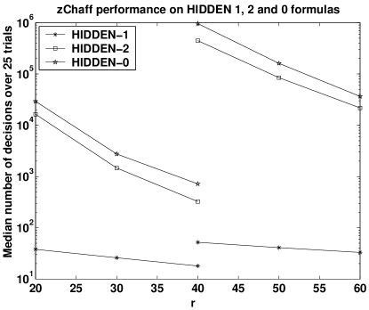
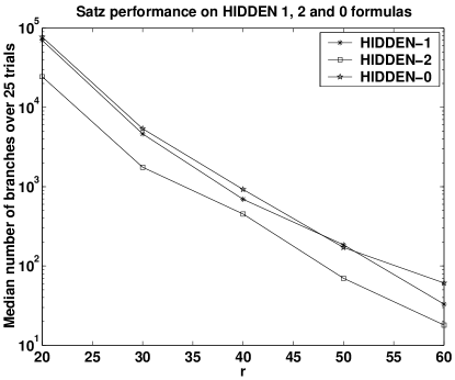
Figure 2: The median number of branchings made by zChaff and Satz  on random instances with 0, 1, and 2 hidden assignments (on a $\log_{10}$ scale). For zChaff we use $n=1000$ for $r=20,30,40$ and $n=3000$ for $r=40,50,60$, and for Satz we use $n=3000$ throughout. Each point is the median of 25 trials. The 2-hidden formulas are almost as hard for both algorithms as the 0-hidden ones, while the 1-hidden formulas are much easier for zChaff.

4.2 SP

SP is an incomplete solver recently introduced by Mézard and Zecchina [24] based on a generalization of belief propagation the authors call survey propagation. It is inspired by the physical notion of “replica symmetry breaking” and the observation that for $3.9<r<4.25$, random 3-SAT formulas appear to be satisfiable, but their satisfying assignments appear to be organized into clumps.

In Figure 3 we compare SP’s performance on the three types of problems near the satisfiability threshold. For $n=10^{4}$ SP solves 2-hidden formulas at densities somewhat above the threshold, up to $r\approx 4.8$, while it solves the 1-hidden formulas at still higher densities, up to $r\approx 5.6$.

Presumably the 1-hidden formulas are easier for SP since the “messages” from clauses to variables, like the majority heuristic, tend to push the algorithm towards a hidden assignment. Having two hidden assignments appears to cancel these messages out to some extent, causing SP to fail at a lower density. However, this argument does not explain why the SP-threshold for 2-hidden formulas should be higher than the satisfiability threshold; nor does it explain why SP does not solve 1-hidden formulas for arbitrarily large $r$. Indeed, we find this latter result surprising, since as $r$ increases the majority of clauses should point more and more consistently towards the hidden assignment in the 1-hidden case.

We note that we also performed the above experiments with $n=2\times 10^{4}$ and with $5000$ iterations, instead of the default $1000$, for SP’s convergence procedure. The thresholds of Figure 3 for 1-hidden and 2-hidden formulas appeared to be stable under both these changes, suggesting that they are not merely artifacts of our particular experiments. We propose investigating these thresholds as a direction for further work.

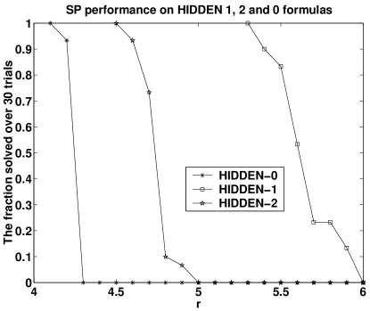
Figure 3: The fraction of problems successfully solved by SP as a function of density, with $n=10^{4}$ and $30$ trials for each value of $r$. The threshold for solving 2-hidden formulas is somewhat higher than for 0-hidden ones, and for 1-hidden formulas it is higher still.

4.3 WalkSAT

We conclude with a local search algorithm, WalkSAT. Unlike the complete solvers, WalkSAT can solve problems with $n=10^{4}$ fairly close to the threshold. We performed experiments both with a random initial state, and with a biased initial state where the algorithm starts with $75\%$ agreement with one of the hidden assignments (note that this is exponentially unlikely). In both cases, we performed trials of $10^{8}$ flips for each formula, without random restarts, where each step does a random or greedy flip with equal probability. Since random initial states w.h.p. have roughly $50\%$ agreement with both hidden assignments, we expect their attractions to cancel out so that WalkSAT will have difficulty finding either of them. On the other hand, if we begin with a biased initial state, then the attraction from the nearby assignment will be much stronger than the other one; this situation is similar to a 1-hidden formula, and we expect WalkSAT to find it easily. Indeed our data confirms these expectations.

In the first part of Figure 4 we measure WalkSAT’s performance on the three types of problems with $n=10^{4}$ and $r$ ranging from $3.7$ to $5.5$, and compare them with 0-hidden formulas for $r$ ranging from $3.7$ up to $4.1$, just below the threshold where they become unsatisfiable. We see that, below the threshold, the 2-hidden formulas are just as hard as the 0-hidden ones when WalkSAT sets its initial state randomly; indeed, their running times coincide to within the resolution of the figure! They both become hardest when $r\approx 4.2$, where $10^{8}$ flips no longer suffice to solve them.

On the other hand, the 1-hidden formulas are much easier than the 2-hidden ones, and their running time peaks around $r=5.2$. Finally, the 2-hidden formulas are much easier to solve when we start with a biased initial state, in which case the running time is closer to that of 1-hidden formulas.

In the second part of Figure 4, we compare the three types of formulas at a density very close to the threshold, $r=4.25$, and measure their running times as a function of $n$. The data suggests that 2-hidden formulas with random initial states are much harder than 1-hidden ones, while 2-hidden formulas with biased initial states have running times within a constant of that of 1-hidden formulas. (Note that, consistent with experiments of [8], the median running time of all three types of problems is polynomial in $n$.)

Based on this, we conjecture the following. Our 2-hidden formulas are just as hard for WalkSAT as 0-hidden ones up to the satisfiability threshold, and they are hardest at or near the threshold. Moreover, they are much harder than 1-hidden formulas, unless WalkSAT is lucky enough to have an initial state biased towards one of the hidden assignments.

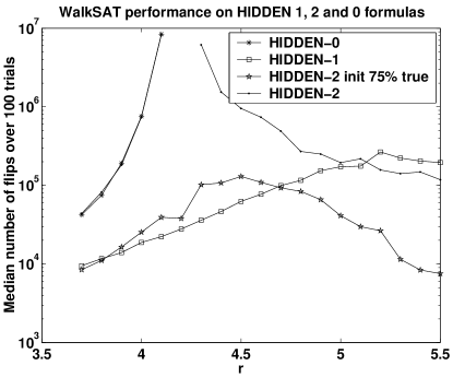
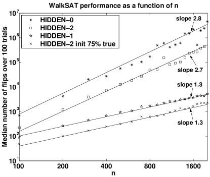
Figure 4: Left, the median number of flips needed by WalkSAT for formulas of all three types below and above the threshold, with $n=10^{4}$. Below the threshold, 2-hidden formulas are just as hard as 0-hidden ones (they coincide to within the resolution of the figure) and their running time increases steeply as we approach the threshold. Both above and below the threshold, 2-hidden formulas are much harder than 1-hidden ones, unless the algorithm starts with a (exponentially lucky) biased initial state. Right, the median number of flips needed by WalkSAT to solve the three types of formulas at $r=4.25$ as a function of $n$. Here $n$ ranges from $100$ to $2000$. While the median running time for all three is polynomial, the 2-hidden problems are much harder than the 1-hidden ones unless the have a biased initial state, with a running time that scales similarly to 0-hidden problems, i.e., random 3-SAT.

5 Conclusions

We have introduced an extremely simple new generator of random satisfiable 3-SAT instances which is amenable to all the mathematical tools developed for the rigorous study of random 3-SAT instances. Experimentally, our generator appears to produce instances that are as hard as random 3-SAT instances, in sharp contrast to instances with a single hidden assignment. This hardness appears quite robust; our experiments have demonstrated it both above and below the satisfiability threshold, and for algorithms that use very different strategies, i.e., DPLL solvers (zChaff and Satz), local search algorithms (WalkSAT), and survey propagation (SP).

We believe that random 2-hidden instances could make excellent satisfiable benchmarks, especially just around the satisfiability threshold, say at $r=4.25$ where they appear to be the hardest for WalkSAT (although beating SP requires somewhat higher densities).

Several aspects of our experiments suggest exciting directions for further work, including:

1. Proving that the expected running time of natural Davis-Putnam algorithms on 2-hidden formulas is exponential in $n$ for $r$ above some critical density.

2. Explaining the different threshold behaviors of SP on 1-hidden and 2-hidden formulas.

3. Understanding how long WalkSAT takes at the midpoint between the two hidden assignments, before it becomes sufficiently unbalanced to converge to one of them.

4. Studying random 2-hidden formulas in the dense case where there are $\omega(n)$ clauses.

References

- [1] D. Achlioptas, Lower bounds for random 3-sat via differential equations, Theor. Comp. Sci. 265 (2001), 159–185.
- [2] D. Achlioptas, P. Beame, and M. Molloy, A sharp threshold in proof complexity, STOC (2001), 337–346.
- [3] D. Achlioptas, C. Gomes, H. Kautz, and B. Selman, Generating satisfiable problem instances, AAAI (2000), 256–261.
- [4] D. Achlioptas and C. Moore, Two moments suffice to cross a sharp threshold, SIAM J. Comput., to appear.
- [5] , Almost all graphs with average degree 4 are 3-colorable, STOC (2002), 199–208.
- [6] , The asymptotic order of the random -sat threshold, FOCS (2002), 779–788.
- [7] Y. Asahiro, K. Iwama, and E. Miyano, Random generation of test instances with controlled attributes, DIMACS Series in Disc. Math. and Theor. Comp. Sci. 26 (1996), 377–393.
- [8] W. Barthel, A.K. Hartmann, M. Leone, F. Ricci-Tersenghi, M. Weigt, and R. Zecchina, Hiding solutions in random satisfiability problems: A statistical mechanics approach, Phys. Rev. Lett 88 (2002), no. 188701.
- [9] M.T. Chao and J. Franco, Probabilistic analysis of two heuristics for the 3-satisfiability problem, SIAM J. Comput. 15 (1986), no. 4, 1106–1118.
- [10] P. Cheeseman, R. Kanefsky, and W. Taylor, Where the really hard problems are, IJCAI (1991), 163–169.
- [11] S. Cocco and R. Monasson, Statistical physics analysis of the computational complexity of solving random satisfiability problems using backtrack algorithms, Eur. Phys. J. B 22 (2001), 505–531.
- [12] S. Coco and R. Monasson, Trajectories in phase diagrams, growth processes and computational complexity: how search algorithms solve the 3-satisfiability problem, Physical Review Letters 86 (2001), 1654–1657.
- [13] D.J. Du, J. Gu, and P. Pardalos, Dimacs workshop on the satisfiability problem, 1996, vol. 35, AMS, 1997.
- [14] M. Hajiaghayi and G.B. Sorkin, The satisfiability threshold for random 3-sat is at least 3.52, 2003.
- [15] T. Hogg, B.A. Huberman, and C.P. Williams, Phase transitions and complexity, Artificial Intelligence 81 (1996), special issue.
- [16] D. Johnson and M. Trick, Second dimacs implementation challenge, 1993, DIMACS Series in Disc. Math. and Theor. Comp. Sci., vol. 26, 1996.
- [17] D.S. Johnson, C.R. Aragon, L.A. McGeoch, and C. Shevon, Optimization by simulated annealing: an experimental evaluation, Operations Research 37 (1989), no. 6, 865–892.
- [18] AC. Kaporis, L.M. Kirousis, and E.G. Lalas, Selecting complementary pairs of literals, Proceedings of LICS Workshop on Typical Case Complexity and Phase Transitions (2003).
- [19] H. Kautz, Y.l. Ruan, D. Achlioptas, C. Gomes, B. Selman, and M. Stickel, Balance and filtering in structured satisfiable problems, IJCAI (2001), 351–358.
- [20] L.M. Kirousis, E. Kranakis, D. Krizanc, and Y. Stamatiou, Approximating the unsatisfiability threshold of random formulas, Random Structures Algorithms 12 (1998), no. 3, 253–269.
- [21] C.M. Li and Anbulagan, Heuristics based on unit propagation for satisfiability problems, IJCAI (1997), 366–371.
- [22] , Look-ahead versus look-back for satisfiability problems, 3rd Intl. Conf. on Principles and Practice of Constraint Programming (1997), 341–355.
- [23] F. Massacci, Using walk-sat and rel-sat for cyptographic key search, IJCAI (1999), 290–295.
- [24] M. Mézard and R. Zecchina, Random k-satisfiability: from an analytic solution to a new efficient algorithm, Phys. Rev. E 66 (2002), Available at: http://www.ictp.trieste.it/~zecchina/SP/.
- [25] D. Mitchell, B. Selman, and H.J. Levesque, Hard and easy distributions of sat problems, AAAI (1992), 459–465.
- [26] P. Morris, The breakout method for escaping from local minima, AAAI (1993), 40–45.
- [27] M. Moskewicz, C. Madigan, Y. Zhao, L. Zhang, and S. Malik, Chaff: engineering an efficient sat solver, 38th Design Automation Conference (2001), 530–535.
- [28] B. Selman, H.A. Kautz, and B. Cohen, Local search strategies for satisfiability testing, 2nd DIMACS Challange on Cliques, Coloring, and Satisfiability (1996).
- [29] P. Shaw, K. Stergiou, and T. Walsh, Arc consistency and quasigroup completion, ECAI, workshop on binary constraints (1998).
- [30] A. Van Gelder, Problem generator mkcnf.c, DIMACS (1993), Challenge archive.
- [31] N.C. Wormald, Differential equations for random processes and random graphs, Ann. Appl. Probab. 5 (1995), no. 4, 1217–1235.