Uplink Throughput in a Single-Macrocell/Single-Microcell CDMA System, with Application to Data Access Points

Abstract

This paper studies a two-tier CDMA system in which the microcell base is converted into a data access point (DAP), i.e., a limited-range base station that provides high-speed access to one user at a time. The microcell (or DAP) user operates on the same frequency as the macrocell users and has the same chip rate. However, it adapts its spreading factor, and thus its data rate, in accordance with interference conditions. By contrast, the macrocell serves multiple simultaneous data users, each with the same fixed rate. The achieveable throughput for individual microcell users is examined and a simple, accurate approximation for its probability distribution is presented. Computations for average throughputs, both per-user and total, are also presented. The numerical results highlight the impact of a desensitivity parameter used in the base-selection process.

I Introduction

In [1], we studied the uplink user capacity in a two-tier CDMA system composed of a single macrocell within which a single microcell is embedded. This system assumed that all users transmit over the same set of frequencies, with handoff between tiers. Analytical techniques were developed to both exactly compute and accurately approximate the user capacity supported in such a two-tier system. Here, we implement these techniques to study a particular kind of single-macrocell/single-microcell system. Specifically, we consider a wireless data system where the microcell is designed to attract only a small number of users $(n)$, while the macrocell attracts a larger number of users $(N_{M})$. The users are uniformly distributed over the entire system coverage area, all having the same chip rate, $1/W$, where $W$ is the system bandwidth. The macrocell users have the same fixed data rate, $R_{M}$, and the same output signal-to-interference-plus-noise ratio (SINR) requirement, $\Gamma_{M}$. The $n$ microcell users, on the other hand, can be high-speed and are given access to the microcell one-at-a-time. The microcell resembles a data access point (DAP), i.e., a base station with limited coverage area that provides high data rates to a small number of users in sequence. Some examples of DAP-like applications are in [2]-[5]. The uplink data rate, $R_{\mu}$, of any given microcell user has a maximum achieveable value, $R_{\mu}^{*}$, determined by existing interference conditions. We will quantify $R_{\mu}^{*}$ and related quantities for a given a microcell output SINR requirement. We focus here on the uplink, which we have shown in [6] to be the limiting direction in this kind of architecture.

In Section II, we elaborate on the system architecture, the uplink SINR’s, and the path gain model used. In the process, we identify a normalized desensitivity factor, $\zeta$, that is a key design variable. In Section III, we derive the uplink transmission rate for a given user and propose (and confirm via simulation) a simple approximation for its probability distribution. In Section IV, we compute, as functions of $\zeta$, the average per-user and per-DAP throughputs and show that the choice of $\zeta$ involves a tradeoff between user high-speed capability and overall DAP utilization. We also show the tradeoff between DAP performance and total user population.

II System and Channel Assumptions

II-A Architecture

We assume a system in which $N$ data users in some region $\mathcal{R}$ communicate with either a low-speed macrocell base or a microcell base acting as a DAP, as shown in Fig. 1. In our computations, we will further assume that the region $\mathcal{R}$ is a square of side $L$, with the macrocell base at its center, the microcell base at some distance $D$ from the center, and users located with uniform randomness over the region.

Each data user communicates with the macrocell at a fixed rate $R_{M}=W/G$, where $G$ is the spreading factor of the CDMA code. However, when a user’s path gain to the microcell base (DAP) exceeds some threshold, it becomes a candidate for communication, at higher speed, with the DAP. The base selection criterion we use is that the macrocell base is selected whenever the user’s path gain to it exceeds that to the DAP by some fraction $\delta$, called the desensitivity factor, or just desensitivity. Clearly, the smaller $\delta$ is, the smaller the number of users eligible for DAP access.

We denote by $n$ the number of eligible DAP users at any time, and specify that they access the DAP sequentially. Each gets a timeslot whose duty cycle is $1/n$, and a data rate during the timeslot that depends on factors discussed below. The remaining $N_{M}=N-n$ users simultaneously access the macrocell base at data rate $R_{M}$. These users require a minimum SINR of $\Gamma_{M}$ while each of the $n$ DAP users requires a minimum SINR of $\Gamma_{\mu}$.

II-B Uplink SINR’s

Each of the $n$ microcells users accesses the microcell one-at-a-time so that, at any one time, there are exactly $N_{M}+1$ system users. The base stations employ matched filter (RAKE) receivers to detect these active users. Each base controls the transmit powers of its own users so that each user meets the minimum output SINR requirement at that base. For such a system, the output SINR’s at the macrocell and microcell are

$$\mbox{SINR}_{M}=\frac{\frac{W}{R_{M}}S_{M}}{(N_{M}-1)S_{M}+S_{\mu}I_{M}+\eta W}$$ (1)

and

$$\mbox{SINR}_{\mu}=\frac{\frac{W}{R_{\mu}}S_{\mu}}{S_{M}I_{\mu}+\eta W},$$ (2)

respectively, where $S_{M}$ and $S_{\mu}$ are the received power from each macrocell user at the macrocell base and the received power from the microcell user at the microcell base, respectively; $\eta W$ is the received noise power, at each base, in bandwidth $W$; $R_{M}$ and $R_{\mu}$ are the bit rates of macrocell and microcell users, respectively; and $I_{M}$ and $I_{\mu}$ are the normalized cross-tier interferences. Specifically, $I_{\mu}$ is the normalized interference from the $N_{M}$ macrocell users into the microcell base, and $I_{M}$ is the normalized interference from the one active microcell user into the macrocell base. As shown in [1], $I_{\mu}$ and $I_{M}$ depend solely on the set of path gains from the active users to both bases, and on $\delta$. They are

$$I_{M}=\frac{T_{M}}{T_{\mu}}$$ (3)

and

$$I_{\mu}=\sum_{k\in M}\frac{T_{\mu k}}{T_{Mk}},$$ (4)

where $T_{M}$ ($T_{\mu}$) is the path gain from the microcell user to the macrocell (microcell) base; $T_{\mu k}$ ($T_{Mk}$) is the path gain from the $k$-th macrocell user to the microcell (macrocell) base; and $M$ denotes the set of all macrocell users. The denominators in (3) and in each term of (4) are a consequence of using power control to each user from its serving base. Adequate performance requires that $\mbox{SINR}_{M}\geq\Gamma_{M}$ and $\mbox{SINR}_{\mu}\geq\Gamma_{\mu}$.

II-C Path Gain Model

The path gain, $T$, between either base and a user at a distance $d$ is assumed to be

$$T=\left\{\begin{array}[]{cc}H\left(\frac{b}{d}\right)^{2}10^{\chi/10},&d\leq b\\ H\left(\frac{b}{d}\right)^{4}10^{\chi/10},&d>b\end{array}\right.,$$ (7)

where $b$ is the “breakpoint distance” (in the same units as $d$), at which the slope of the dB path gain versus distance changes; $\chi$ is a zero-mean Gaussian random variable for each user position, with standard deviation $\sigma$; and $H$ is a proportionality constant that depends on wavelength, antenna heights and antenna gains. Note that $T$ is a local spatial average, so that multipath effects are averaged out. There can be different values of $b$ for the microcell and macrocell, and similarly for $\sigma$ and $H$. The factor $10^{\chi/10}$ is often referred to as lognormal shadow fading, which varies slowly over the terrain. Both $\chi$ and $d$ are random variables for a randomly selected user.

Due to the greater height and gain of the typical macrocell antenna, we can assume $H_{M}>H_{\mu}$. As mentioned above, the system we examine here assumes path-gain-based selection, i.e., a user selects the macrocell base if the path gain to it exceeds the path gain to the microcell base by some specified fraction $\delta$. In addition, the path gain of a user to the macrocell exceeds its path gain to the microcell by a value $h=H_{M}/H_{\mu}$ for the same distance and shadow fading. Therefore, base selection depends fundamentally on the ratio $\delta/h$, as opposed to $\delta$ alone. (We chose not to normalize $\delta$ by $h$ in our study in [1].) The factor $\delta/h$ is called the normalized desensitivity of the microcell, and is hereafter denoted by $\zeta$. Smaller values of $\zeta$ correspond to higher path gain requirements to the microcell. This means that outlying users are generally excluded from access to the microcell, and a smaller microcell coverage area results.

III Data Rate for a DAP User

For a given number of DAP users $n$, we have $N_{M}=N-n$ macrocell users, and there is a probability $p_{n}$ (derivable from the results in [1]) that $n$ of the $N$ users will choose the microcell and $N-n$ the macrocell. We can show from (1) and (2) that the requirements $\mbox{SINR}_{M}\geq\Gamma_{M}$ and $\mbox{SINR}_{\mu}\geq\Gamma_{\mu}$ yield positive solutions for $S_{\mu}$ and $S_{M}$ if and only if

$$\frac{W}{R_{\mu}}(K-N_{M})-\Gamma_{\mu}I_{M}I_{\mu}\geq 0,$$ (8)

where $K=W/(R_{M}\Gamma_{M})+1$ is the single-cell pole capacity of the macrocell [7]. Thus, we can find $R_{\mu}^{*}(n)$, the maximum achieveable $R_{\mu}$ when $n$ users choose the microcell: Using (8) with $N_{M}=N-n$, and noting that the spreading factor $W/R_{\mu}$ cannot be less than 1, we have

$$R_{\mu}^{*}(n)=\min\left(\frac{W(K-N+n)}{\Gamma_{\mu}I_{M}I_{\mu}},W\right),\mbox{~{}~{}~{}}1\leq n\leq N.$$ (9)

We define $r=R_{\mu}^{*}/W$ and, henceforth, we examine this normalized data rate. Note that $r$ will be different as each of the $n$ users takes its turn, because $I_{M}I_{\mu}$ depends on the set of all (active) user path gains. Also, for any given user, we see that $I_{M}$ and $I_{\mu}$ are random variables because of the random locations and shadow fadings of all users. Thus, $r$ is itself a random variable. To facilitate analysis, we assume (and will show) that $I_{M}$ and $I_{\mu}$ can be treated as lognormal variates, whose first and second moments are obtainable using the results in [8]. Since $1/(I_{M}I_{\mu})$ is lognormal under this assumption, we conclude that $r$, as given above, is a truncated lognormal random variable. The Appendix shows how the lognormal parameters are obtained from the moments of $I_{M}$ and $I_{\mu}$.

Let $F(r|n)$ denote the cumulative distribution function (CDF) of $r$ for a given $n$. The CDF of $r$ with the condition on $n$ removed, but subject to $n$ exceeding 0, is

$$F(r)=\frac{\sum_{n=1}^{N}p_{n}F(r|n)}{1-p_{0}}.$$ (10)

Assuming that $F(r|n)$ can be approximated as the CDF of a truncated lognormal random variable, $F(r)$ can approximated by a weighted sum of CDF’s of truncated lognormals.

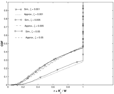
Figure 2: CDF’s of $r$ using both simulation and the approximation method, for $\zeta=0.001$, $0.005$ and $0.05$. Results are for $N=26$.

To test the reliability of the lognormal approximation, we performed a series of simulation trials. We assumed a square region $\mathcal{R}$ with sides of length $L$ over which users are uniformly distributed, with the two bases separated by $D$. For the system and propagation parameters listed in Table 1, we determined the achieveable data rates of microcell users over 10,000 trials, for various values of $\zeta$ and with $N=26$. The resulting CDF of $r$ is plotted in Fig. 2. Along with simulation results, this figure contains CDFs obtained from analysis, (10), assuming lognormal cross-tier interferences. These results show that the lognormal approximation is reliable over a wide range of $\zeta$. As $\zeta$ gets smaller, the data rates of the microcell users increase, suggesting that smaller $\zeta$ is desirable. The problem with extremely small $\zeta$, however, is that it shrinks the population of possible microcell users. The result is under-utilization of the DAP, as discussed below.

IV Results

IV-A Per-User and Total DAP Throughputs

We define our throughput variable as the time-averaged data rate normalized by $W$. The per-user throughput, $\tau_{u}$, takes into account the time-limited access that data users must accept if there is more than one microcell user in the system. This division of time effectively reduces data rates $(r)$ in a system with $n$ microcell users by a factor of $n$. The CDF of $\tau_{u}$ is thus

$$F_{\tau_{u}}(\tau_{u})=\frac{\sum_{n=1}^{N}p_{n}F(n\tau_{u}|n)}{1-p_{0}},$$ (11)

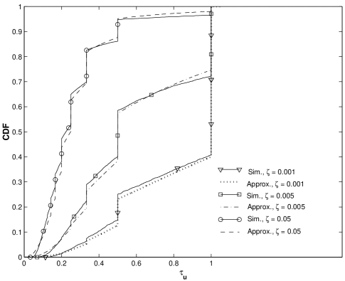
Figure 3: CDF of $\tau_{u}$ using both simulation and the approximation method, for $\zeta=0.001$, $0.005$ and $0.05$. Results are for $N=26$.

where $F(\cdot|n)$ is as defined earlier. The CDF of $\tau_{u}$ can be approximated using the truncated-lognormal assumption for $R_{\mu}^{*}$, (9). Using both simulation and this approximation, we again considered the single-macrocell/single-microcell system described above, with the parameters in Table 1. The results are plotted in Fig. 3 for three different values of $\zeta$. We see that the approximate distribution follows the simulation distribution very closely for all three values. The jumps in Fig. 3 are related to the fact that per-user data rates are confined to the discrete values $W/n$, $n=1,2,\ldots$ for the high fraction of cases where $R^{*}_{\mu}=W$.

The total throughput for the DAP, for given a $n\geq 0$, is the sum of the throughputs for the $n$ users. We denote the total throughput (i.e., DAP utilization) by $\tau_{d}$. Thus, $\tau_{d}$ represents performance from the network operator’s point-of-view, while $\tau_{u}$ represents performance from the user’s point-of-view. We quantify the average per-user and per-DAP throughputs, as functions of $\zeta$, where the averaging is over random locations and shadow fadings of the users. $\mbox{E}\{\tau_{u}\}$ is obtained via the formula for its CDF, (11). $\mbox{E}\{\tau_{d}\}$ is obtained by noting that $\mbox{E}\{\tau_{d}|n\}$ is just $\mbox{E}\{r|n\}$. Removing the condition on $n$, we get

$$\mbox{E}\{\tau_{d}\}=\sum_{n=0}^{N}p_{n}\mbox{E}\{r|n\}.$$ (12)

The results for $\mbox{E}\{\tau_{u}\}$ and $\mbox{E}\{\tau_{d}\}$ are shown in Fig. 4 for $N=26$. They are given for both simulation and the approximation method, and we see very strong agreement. For this system, we see that, when $\zeta\approx 0.007$, $\mbox{E}\{\tau_{u}\}=\mbox{E}\{\tau_{d}\}\equiv\tau^{*}$. This value of $\zeta$ (which we call $\zeta^{*}$) is desirable, since it balances the throughput for both individual users and the overall DAP. When $\zeta>\zeta^{*}$, individual user throughputs are compromised for the sake of higher DAP utilization; when $\zeta<\zeta^{*}$, higher per-user throughputs are obtained, but for an under-utilized DAP.

IV-B Effect of $N$ on $\tau^{*}$

The results reported thus far assumed $N=26$, i.e., $N\approx K$. It is instructive to repeat the above exercise for a range of $N$, to show the tradeoff between total user population and DAP throughput. Thus, we have computed $\mbox{E}\{\tau_{u}\}$ and $\mbox{E}\{\tau_{d}\}$ as functions of $\zeta$ for various $N$, still assuming a uniform distribution of users. For each value of $N$, $\mbox{E}\{\tau_{u}\}$ decreases and $\mbox{E}\{\tau_{d}\}$ increases with increasing $\zeta$, just as in Fig. 4; however, the values of $\tau^{*}$ and $\zeta^{*}$ change with $N$. This is shown in Fig. 5.

For a given $\zeta$, decreasing $N$ implies a shrinking number of DAP users, leading to a less utilized DAP. Thus, $\zeta$ must be increased to maintain high DAP utility, i.e., $\zeta^{*}$ must increase as $N$ decreases below $K$. At the same time, the cross-tier interference at the DAP shrinks, leading to increases in $\tau^{*}$. In the region $N\leq K$, the average $n$ at $\zeta=\zeta^{*}$ is close to 1, so that $N_{M}\approx N-1$. In the region $N>K$, meeting the feasibility condition $N_{M}<K$, (6), requires that $n>1$. The result is a sharp decline in $\tau^{*}$ as $N$ increases from $K$, as foretold by the steepness of the $\tau^{*}$-curve at $N=26$.

IV-C Effect of Dense User Distribution Around the DAP

Using the methods presented here, throughput results can be obtained for a system with a denser user distribution around the DAP. We found that, as the density around the DAP increases, both $\zeta^{*}$ and $\tau^{*}$ decrease. Smaller values of $\zeta^{*}$ are desirable because they help reduce $n$, the number of users that must share the DAP. Despite this, as the user density around the DAP increases, the most probable value of $n$ increases, resulting in smaller $\tau_{u}$ and a net (modest) reduction in $\tau^{*}$.

V Conclusion

We have demonstrated that by controlling the desensitivity factor, a microcell can be converted to a data access point. The data rate of the single DAP user was analyzed and shown to be well-represented as a truncated-lognormal variate. A method was then developed to compute the throughput statistics, and we found values of desensitivity, over the practical range of user population, for which both per-user and total DAP throughputs are reasonably high.

Appendix A Lognormal Representation of the User Data Rate

The user data rate, $r=R_{\mu}^{*}/W$ is seen from (9) to be the lesser of 1 and $Z$, where $Z=(K-N-n)/(\Gamma_{\mu}I_{M}I_{\mu})$. Defining $z=\ln Z$, we have $z=\ln((K-N-n)/\Gamma_{\mu})-\ln I_{M}-\ln I_{\mu}$. Clearly, if $I_{M}$ and $I_{\mu}$ are lognormal, $z$ is a Gaussian random variable whose mean and standard deviation are obtainable from the means and standard deviations of $\ln I_{M}$ and $\ln I_{\mu}$.

In [8], the first and second moments of $I_{M}$ and $I_{\mu}$ are derived for the two-cell system. The means and standard deviations of $\ln I_{M}$ and $\ln I_{\mu}$ are then obtainable as follows: Let the mean and standard deviation of $\ln I_{M}$ be $m$ and $\sigma$, respectively. From lognormal statistics [9], [10],

$$\mbox{E}\{I_{M}\}=e^{m}e^{\sigma^{2}/2}\mbox{~{}~{}~{}and~{}~{}~{}~{}}\mbox{E}\{I_{M}^{2}\}=e^{2m}e^{2\sigma^{2}}.$$

Solving for $m$ and $\sigma$,

$$m=\frac{1}{2}\ln\left(\frac{(\mbox{E}\{I_{M}\})^{4}}{\mbox{E}\{I_{M}^{2}\}}\right)\mbox{~{}~{};~{}~{}~{}}\sigma=\sqrt{\ln\left(\frac{\mbox{E}\{I_{M}^{2}\}}{(\mbox{E}\{I_{M}\})^{2}}\right)}.$$

Similar results apply to $\ln I_{\mu}$. Thus, $r$ can be fully described as a truncated lognormal variate given the first two moments of $I_{M}$ and $I_{\mu}$, and assuming both are lognormal.

$W/R_{M}$	128	$L$	1 km
$\Gamma_{M}$	7 dB	$\Gamma_{\mu}$	8.45 dB
$b_{M}$	100 m	$b_{\mu}$	100 m
$H_{M}$	$10H_{\mu}$	$D$	300 m
$\sigma_{M}$	8 dB	$\sigma_{\mu}$	4 dB

TABLE I: System Parameters Used

Figure 1: An example of a region $\mathcal{R}$, with macrocell and microcell base station. Here M BS and $\mu$ BS denote the macrocell and microcell base stations, respectively.

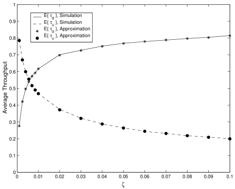
Figure 4: $\mbox{E}\{\tau_{u}\}$ and $\mbox{E}\{\tau_{d}\}$ as functions of $\zeta$ using both simulation and the approximation method. Results are for $N=26$.

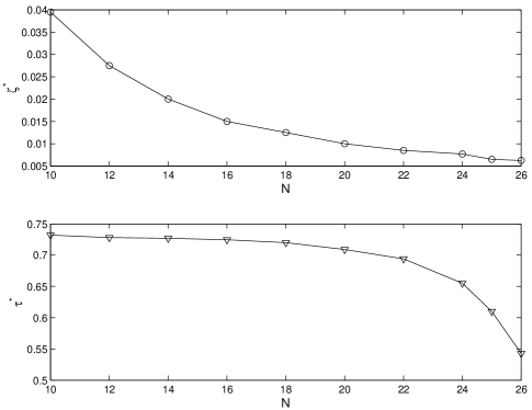
Figure 5: $\zeta^{*}$ and $\tau^{*}$ as functions of $N$, for $10\leq N\leq K$.

References

- [1] S. Kishore, et al., “Uplink Capacity in a CDMA Macrocell with a Hotspot Microcell: Exact and Approximate Analyses,” IEEE Transactions on Wireless Communications, Vol. 2, No. 2, pp. 364-374, March 2003.
- [2] R. Kohno, “ITS and Mobile Multi-Media Communication in Japan,” Proc. of Telecommunication Technique Workshop for ITS, Seoul, Korea, pp. 9-33, May 2000.
- [3] B.S. Lee, et al., “Performance Evaluation of the Physical Layer of the DSRC Operating in 5.8 GHz Frequency Band” ETRI Journal, Vol. 23, No. 3, pp. 121-128, September 2001.
- [4] R. Frenkiel and T. Imielinski, “Infostations: The Joy of Many-Time, Many-Where Communications,” WINLAB Technical Report, TR-119, Rutgers University, 1996.
- [5] D. Goodman, et al., “Infostations: A New System Model for Data and Messaging Services,” Proceedings of the 1997 IEEE Vehicular Techn. Conf., Phoenix, AZ, pp. 969-973, May 1997.
- [6] S. Kishore, et al., “Downlink User Capacity in a CDMA Macrocell with a Hotspot Microcell,” in Proceedings of IEEE Globecom, vol. 3, pp. 1573-1577, December 2003.
- [7] K.S. Gilhousen, et al., “On the Capacity of a Cellular CDMA System,” IEEE Transactions on Vehicular Technology, Vol. 40, pp. 303-312, May 1991.
- [8] S. Kishore, “Capacity and Coverage of Two-Tier Cellular CDMA Networks,” Ph.D. Thesis, Department of Electrical Engineering, Princeton University, January 2003, Appendix B.
- [9] A. J. Goldsmith, et al., “Error Statistics of Real-Time Power Measurements in Cellular Channels with Multipath and Shadowing,” IEEE Transactions on Vehicular Technology, Vol. 43, No. 3, pp. 439-446, August 1994.
- [10] S.C. Schwartz and Y.S. Yeh, “On the Distribution Function and Moments of Power Sums with Lognormal Components,” Bell System Technical Journal, Vol. 61, No. 7, September 1982, pp. 1441-1462.