Approximation of Dynamical Systems using S-Systems Theory: Application to Biological Systems

Abstract

In this article we propose a new symbolic-numeric algorithm to find positive equilibria of a $n$-dimensional dynamical system. This algorithm implies a symbolic manipulation of ODE in order to give a local approximation of differential equations with power-law dynamics (S-systems). A numerical calculus is then needed to converge towards an equilibrium, giving at the same time a S-system approximating the initial system around this equilibrium. This algorithm is applied to a real biological example in 14 dimensions which is a subsystem of a metabolic pathway in Arabidopsis Thaliana.

1 Introduction

The modelling and study of biological or biochemical systems has become an exciting challenge in applied mathematics. The complexity of real biological dynamical systems lies essentially in the non-linearities of the dynamics as well as in the huge dimension of systems, often leading to a numerical approach. However, as the understanding of cellular mechanisms grows, it has become obvious that the modelling step strongly needs symbolic tools in order to manipulate more and more information and data, and to improve computational tools. Therefore a new area emerged, called ”systems biology”. It involves different fields of applied mathematics, from computer algebra (see for instance [10]) to numerical computation ([7]).
In the past decades, a lot of different frameworks have been developped to study behaviors of complex biochemical processes. Let us cite here three of them: the discrete networks (see the work of R. Thomas [15]), the piecewise linear systems (the so-called Glass networks [6], see also [5]) and sigmoidal switch systems ([12]). The main goal of all these approaches is to propose a (more or less) generic class of dynamical systems, either discrete or differential, that model some behaviors of complex interaction systems. Once this class is clearly defined, its mathematical relevance generally allows both theoretical and numerical analysis.
The class of systems we use in this paper is the set of S-systems (see [1], [16], [17]). The basic idea of this model is to represent interactions between biochemical species with power-law dynamics. Their mathematical expression is quite general, but sufficiently simple to allow theoretical and practical investigations. We propose in this article a symbolic-numeric algorithm that is based upon S-systems theory. Its goal is to compute the positive equilibria of a $n$-dimensional system of ordinary differential equations (ODE). As it converges towards an equilibrium, it provides a S-system that approaches the original dynamics around this equilibrium. As we will see, the local approximation of some dynamics with power-laws can be made symbolically in any point of the phase space. It can also include treatment of symbolic parameters. However, iterating this process in order to converge towards equilibria needs a numerical computation, which prevents the use of pure symbolic tools to the end.
In the following, we give a definition of the S-system class as it can be found in the litterature(see for instance [16]). We then propose a symbolic-numeric algorithm that computes an iteration leading to the positive equilibria of a dynamical system. We will see an application of this algorithm on a biological example in dimension $14$. We finally conclude with some remarks on our algorithm and some future works.

2 S-systems

2.1 Definition

We give here a definition of the class of S-systems.

Definition 2.1

A $n$-dimensional S-system $S(\alpha,\beta,G,H)$ is a dynamical system defined by the $n$ differential equations:

$$\dot{x_{i}}=\alpha_{i}\prod_{j=1}^{n}x_{j}^{g_{ij}}-\beta_{i}\prod_{j=1}^{n}x_{j}^{h_{ij}}\;,\;\;i=1\dots n$$

with $\alpha=\left(\alpha_{1},\dots,\alpha_{n}\right)\in{(\mathbb{R}^{*}_{+})^{n}}$ , $\beta=\left(\beta_{1}\dots\beta_{n}\right)\in{(\mathbb{R}^{*}_{+})^{n}}$
and $G=\left(g_{ij}\right)_{i,j=1\dots n}\in\mathcal{M}_{n}(\mathbb{R})$, $H=\left(h_{ij}\right)_{i,j=1\dots n}\in\mathcal{M}_{n}(\mathbb{R}).$
$\mathbb{R}^{*}_{+}$ denotes the set of strictly positive real numbers and $\mathcal{M}_{n}(\mathbb{R})$ denotes the set of real square matrices of order $n$.

Let us introduce the vector field $F$ defined on $\Omega={(\mathbb{R}^{*}_{+})^{n}}$:

$$F(x)=\left(\begin{array}[]{c}f_{1}(x_{1},\dots,x_{n})\\ \vdots\\ f_{n}(x_{1},\dots,x_{n})\end{array}\right)$$

with:

$$f_{i}(x_{1}\dots,x_{n})=\alpha_{i}\prod_{j=1}^{n}x_{j}^{g_{ij}}-\beta_{i}\prod_{j=1}^{n}x_{j}^{h_{ij}}\,,\quad i=1\dots n$$

$F$ is $\mathcal{C}^{1}$ and therefore locally lipschitz on the open $\Omega$. Cauchy-Lipschitz theorem ensures the existence and unicity of a maximal solution of $S(\alpha,\beta,G,H)$ in $\Omega$, given any initial condition $x(0)=x^{0}\in\Omega$.

This definition of S-systems with power-law differential equations is strongly linked with equations of chemical kinetics. As an example, if we consider the following chemical pathway:

$$A+2B\stackrel{{\scriptstyle k_{1}}}{{\rightarrow}}C\stackrel{{\scriptstyle k_{2}}}{{\rightarrow}}3D+E$$

then the mass-action law applied to species $C$ gives the equation:

$$\frac{dc}{dt}=k_{1}ab^{2}-k_{2}d^{3}e$$

(capital letters design species and small letters design concentrations)
Therefore in definition 2.1, coefficients $\alpha_{i}$ and $\beta_{i}$ are sometimes called kinetic rates while $g_{ij}$ and $h_{ij}$ are called kinetic orders.

S-systems are part of a broader formalism known as quasi-monomial (QM) systems (see [2]). An interesting result shows that QM systems can be expressed in the form of Lotka-Volterra quadratic systems (see [2] for details).

2.2 Equilibrium points

The study of the phase portrait of a S-system $S(\alpha,\beta,G,H)$ begins with the search for equilibrium points in $\Omega$. To find them, we have to solve the system:

$$\alpha_{i}\prod_{j=1}^{n}x_{j}^{g_{ij}}=\beta_{i}\prod_{j=1}^{n}x_{j}^{h_{ij}}\,,\quad i=1\dots n$$ (1)

In this paper we will use the following notation:
Given a vector $x\in{(\mathbb{R}^{*}_{+})^{n}}$ and a real square matrix $A=\left(a_{ij}\right)_{i,j=1\dots n}$, we define the vector $x^{A}\in{(\mathbb{R}^{*}_{+})^{n}}$ by:

$$(x^{A})_{i}=\prod_{j=1}^{n}x_{j}^{a_{ij}}\,,\quad i=1\dots n$$

With this notation, we can express equation (1) as follows:

$$x^{G-H}=b$$

where $b$ is the vector $\left(\beta_{1}/\alpha_{1},\dots,\beta_{n}/\alpha_{n}\right)$.
Taking the neperian logarithm, this equation leads to:

$$(G-H)\ln x=\ln b$$

(the logarithm is applied to all components of vector, i.e. $\ln x$ is the $n$-dimensional vector $(\ln x_{1},\dots,\ln x_{n})$). Posing $y=\ln x$, we are brought back to the resolution of a $n$-dimensional linear system in $y$.
We have therefore the following proposition:

Proposition 2.1

A S-system $S(\alpha,\beta,G,H)$ has a unique equilibrium $\widetilde{x}$ in $\Omega$ (i.e. a positive equilibrium) if and only if the matrix $(G-H)$ is invertible. $\widetilde{x}$ can be calculated by the formula:

$$\widetilde{x}=b^{(G-H)^{-1}}$$ (2)

2.3 Stability analysis of the equilibrium

The stability analysis of the equilibrium $\widetilde{x}$ uses the study of the spectrum of $J_{F}(\widetilde{x})$ (the jacobian of $F$ in $\widetilde{x}$). The question we tackle here is to find some relationship between the stability of $\widetilde{x}$ and some properties of the matrix $G-H$.
As a motivating example, let us consider the one-dimensional case. A one-dimensional S-system is expressed by a single differential equation:

$$S(\alpha,\beta,g,h)\,:\quad\dot{x}=f(x)=\alpha x^{g}-\beta x^{h}$$

where $\alpha,\beta>0$ and $g,h\in\mathbb{R}$. The positive equilibrium $\widetilde{x}$ of $(S)$ exists and is unique if and only if $g-h\neq 0$. In this case, an obvious calculation leads to:

$$\frac{\partial f}{\partial x}(\widetilde{x})=\alpha\widetilde{x}^{g-1}(g-h)$$

so the stability of $\widetilde{x}$ depends directly on the sign of $g-h$: it is asymptotically stable if $g-h<0$ and unstable if $g-h>0$, regardless of parameters $\alpha$ and $\beta$.

In the $n$-dimensional case, the stability depends on the sign of the real parts of the jacobian’s eigenvalues. Derivating the functions $f_{i}(x_{1}\dots,x_{n})$, we obtain, for $i,j=1\dots n$:

$$\frac{\partial f_{i}}{\partial x_{j}}(\widetilde{x})=\frac{\alpha_{i}}{\widetilde{x}_{j}}\prod_{k=1}^{n}\widetilde{x}_{k}^{g_{ik}}.\,(g_{ij}-h_{ij})$$ (3)

As in one-dimensional case, we thus obtain a formula that links the jacobian of $F$ in $\widetilde{x}$ with the matrix $G-H$. However, it is not trivial to link the spectrum of $J_{F}(\widetilde{x})$ with the spectrum of $G-H$.
Let us recall here the definition of stability of matrices:

Definition 2.2

A real square matrix $A$ of order $n$ is said to be stable (resp. semi-stable) if all its eigenvalues $\lambda_{i}$, $i=1\dots n$, have a negative (resp. non positive) real part.

We could hope that the stability of matrix $G-H$ was sufficient to deduce the stability of $\widetilde{x}$. However this is not true, as we can see in the following example.
For $n=2$, consider the S-system:

$$(S1):\left\{\begin{array}[]{lll}\dot{x}&=&3xy^{2}-2x^{4}\\ \dot{y}&=&4x^{3}y^{4}-x^{5}y^{3}\end{array}\right.$$

we have:

$$\alpha=\left(\begin{array}[]{l}3\\ 4\end{array}\right),\,\beta=\left(\begin{array}[]{l}2\\ 1\end{array}\right),\,G=\left(\begin{array}[]{ll}1&2\\ 3&4\end{array}\right),\,H=\left(\begin{array}[]{ll}4&0\\ 5&3\end{array}\right)$$

The matrix $G-H$ is equal to:

$$G-H=\left(\begin{array}[]{ll}-3&2\\ -2&1\end{array}\right)$$

Its characteristic polynomial is $\chi(\lambda)=(\lambda+1)^{2}$ so the matrix is stable.
Since $G-H$ is invertible, there is a unique equilibrium: $\widetilde{x}=\left(\frac{32}{3},\frac{256}{9}\right)$.We can calculate the two eigenvalues $\lambda_{1}$ and $\lambda_{2}$ of $J_{F}(\widetilde{x})$. We find that $\lambda_{1},\lambda_{2}>0$, implying that $\widetilde{x}$ is an unstable node. As a result, in spite of the stability of matrix $G-H$, the equilibrium $\widetilde{x}$ is unstable.

The stability of $G-H$ is therefore insufficient to deduce the stability of $\widetilde{x}$.
We need a stronger property known as sign stability (see [9],[11]).

Definition 2.3

Two real square matrices of order $n$, $A=\left(a_{ij}\right)_{i,j=1\dots n}$ and $B=\left(b_{ij}\right)_{i,j=1\dots n}$, have the same sign pattern if:

$$\forall\,i,j=1\dots n\,,\;\text{sgn}(a_{ij})=\text{sgn}(b_{ij})$$

The function sgn is the classical signum function:

$$\forall x\in\mathbb{R}\,,\;\text{sgn}(x)=\left\{\begin{array}[]{cl}+1&\text{ if }x>0\\ 0&\text{ if }x=0\\ -1&\text{ if }x<0\\ \end{array}\right.$$

Definition 2.4

A real square matrix $A$ of order $n$ is said to be sign stable (resp. sign semi-stable) if all the matrices that have the same sign pattern are stable (resp. semi-stable) in the sense of definition 2.2.

In [9] we find a characterization of the sign semi-stability:

Theorem 2.1 (Quirk-Ruppert-Maybee)

A real square matrix $A=\left(a_{ij}\right)_{i,j=1\dots n}$ is sign semi-stable if and only if it satisfies the following three conditions:
(i) $\forall\,i=1\dots n\,,\;a_{ii}\leq 0$ (ii) $\forall\,i\neq j\,,\;a_{ij}a_{ji}\leq 0$ (iii) for each sequence of $k\geq 3$ distinct indices $i_{1},\dots,i_{k}$,       we have: $a_{i(1)i(2)}\dots a_{i(k-1)i(k)}a_{i(k)i(1)}=0$
(The third condition is equivalent to the fact that the directed graph associated to $A$ admits no $k$-cycle for $k\geq 3$)

With this notion, we can formulate the following proposition, which links the stability of the equilibrium $\widetilde{x}$ of a S-system with the sign semi-stability of matrix $G-H$:

Proposition 2.2

Let consider a $n$-dimensional S-system $S(\alpha,\beta,G,H)$. We assume that $G-H$ is invertible and we note $\widetilde{x}$ the unique positive equilibrium of $(S)$. We also assume that $\widetilde{x}$ is hyperbolic (i.e. none of the eigenvalues of the jacobian of $F$ in $\widetilde{x}$ have zero real part).
If the matrix $G-H$ is sign semi-stable (i.e. if it verifies the three conditions of theorem 2.1) then, regardless of parameters $\alpha$ and $\beta$, the equilibrium $\widetilde{x}$ is asymptotically stable.

proof.
Let us note $J$ the Jacobian of $F$ in $\widetilde{x}$ and $P$ the matrix $G-H$. The equation 3 yields:

$$\frac{\partial f_{i}}{\partial x_{j}}(\widetilde{x})=\frac{\gamma_{i}}{\widetilde{x}_{j}}p_{ij}$$

with $\gamma_{i}=\alpha_{i}\prod_{k=1}^{n}\widetilde{x}_{k}^{g_{ik}}$. As $\gamma_{i}>0$ and $\widetilde{x}_{j}>0$ for all $i$ and $j$, matrices $J$ and $P$ have the same sign pattern. We can thus deduce that $J$ is semi-stable and as $\widetilde{x}$ is supposed hyperbolic, it is asymptotically stable.

$\Box$

Let us remark that the latter equation gives, in matricial notation:

$$J=\Gamma PD^{-1}$$

where $\Gamma$ and $D$ are diagonal matrices:

$$\Gamma=\left(\begin{array}[]{ccc}\gamma_{1}&&\\ &\ddots&\\ &&\gamma_{n}\end{array}\right)\,,\qquad D=\left(\begin{array}[]{ccc}\widetilde{x}_{1}&&\\ &\ddots&\\ &&\widetilde{x}_{n}\end{array}\right)$$

so $\text{sgn}(\det(J))=\text{sgn}(\det(P))$. As we have supposed that $P$ is invertible, we deduce that $J$ is also invertible and does not have null eigenvalues. So we supposed the hyperbolicity of $\widetilde{x}$ in order to avoid imaginary eigenvalues of $J$.
We can easily verify in the previous example that $G-H$ is stable but not sign semi-stable ($g_{22}-h_{22}=1>0$).

3 Local approximation of dynamical system using S-systems

In this part, we propose an algorithm for approaching the equilibria of a dynamical system using S-systems. Simultaneously, we obtain a S-system that approximates the initial system around the equilibrium.

3.1 Monomial approximation of a positive vector field

(see [17],[14],[16]).
Let’s consider the positive vector field $F:{(\mathbb{R}^{*}_{+})^{n}}\rightarrow{(\mathbb{R}^{*}_{+})^{n}}$.

$$F(x)=\left(\begin{array}[]{c}f_{1}(x_{1},\dots,x_{n})\\ \vdots\\ f_{n}(x_{1},\dots,x_{n})\end{array}\right)$$

We will suppose $F$ sufficiently smooth on ${(\mathbb{R}^{*}_{+})^{n}}$.
Let us define the following change of variables: $y=\ln x$, and express the logarithm of $F(x)$ as a function $G$ of the new variable $y$:

$$\ln F(x)=\ln F(e^{y})=G(y)$$

The function G is sufficiently smooth on ${\mathbb{R}^{n}}$. Given any arbitrary point $y^{0}\in{\mathbb{R}^{n}}$, let us write the Taylor expansion of $g_{i}$ (for $i=1\dots n$) in the neighborhood of $y^{0}$ at the first order:

$$\forall i=1\dots n\,,\;g_{i}(y)=g_{i}(y^{0})+\sum_{j=1}^{n}(y_{j}-y_{j}^{0})\frac{\partial g_{i}}{\partial y_{j}}(y^{0})+o(\parallel y-y^{0}\parallel)$$

We introduce the functions $\tilde{g}_{i}(y)$ for $i=1\dots n$:

$$\forall i=1\dots n\,,\;\tilde{g}_{i}(y)=g_{i}(y^{0})+\sum_{j=1}^{n}(y_{j}-y_{j}^{0})\frac{\partial g_{i}}{\partial y_{j}}(y^{0})$$

and the functions $\tilde{f}_{i}=\exp(\tilde{g}_{i}(y))$:

$$\begin{array}[]{lll}\tilde{f}_{i}(x)&\stackrel{{\scriptstyle def}}{{=}}&e^{\tilde{g_{i}}(y)}\\ &=&e^{g_{i}(y^{0})}\exp\left(\displaystyle\sum_{j=1}^{n}(y_{j}-y_{j}^{0})\frac{\partial g_{i}}{\partial y_{j}}(y^{0})\right)\\ &=&e^{g_{i}(y^{0})}\displaystyle\prod_{j=1}^{n}\exp\left((y_{j}-y_{j}^{0})\frac{\partial g_{i}}{\partial y_{j}}(y^{0})\right)\end{array}$$

As $y=\ln x$ and $g_{i}(y)=\ln f_{i}(x)$, we have:

$$\tilde{f}_{i}(x)=f_{i}(x^{0})\prod_{j=1}^{n}\left(\frac{x_{j}}{x_{j}^{0}}\right)^{\frac{\partial g_{i}}{\partial y_{j}}(y^{0})}$$

and:

$$\begin{array}[]{lll}\displaystyle\frac{\partial g_{i}}{\partial y_{j}}(y)&=&\displaystyle\frac{\partial}{\partial y_{j}}\left(\ln(f_{i}(e^{y}))\right)\\[8.53581pt] {}&=&\displaystyle\frac{1}{f_{i}(e^{y})}\frac{\partial}{\partial y_{j}}\left(f_{i}(e^{y})\right)\\[8.53581pt] {}&=&\displaystyle\frac{1}{f_{i}(x)}e^{y_{j}}\frac{\partial f_{i}}{\partial x_{j}}(e^{y})\\[8.53581pt] {}&=&\displaystyle\frac{x_{j}}{f_{i}(x)}\frac{\partial f_{i}}{\partial x_{j}}(x)\\ \end{array}$$

Therefore, we have defined a vector field $\widetilde{F}=\displaystyle\left(\tilde{f}_{i}\right)_{i=1\dots n}$

$$\widetilde{F}(x)=\left(\alpha_{i}\prod_{j=1}^{n}x_{j}^{g_{ij}}\right)_{i=1\dots n}$$ (4)

$$\text{with: }\left\{\begin{array}[]{lcl}\alpha_{i}(x^{0})&=&\displaystyle f_{i}(x^{0})\prod_{j=1}^{n}(x_{j}^{0})^{-g_{ij}}\\[5.69054pt] {}g_{ij}(x^{0})&=&\displaystyle\frac{x_{j}^{0}}{f_{i}(x^{0})}\frac{\partial f_{i}}{\partial x_{j}}(x^{0})\end{array}\right.$$ (5)

The basic idea is to use the monomial vector field $\widetilde{F}$ as an approximation of $F$ in a neighborhood of $x^{0}$.

Definition 3.1

Let $F$ be a smooth $n$-dimensional vector field, $F:{(\mathbb{R}^{*}_{+})^{n}}\rightarrow{(\mathbb{R}^{*}_{+})^{n}}$ and $x^{0}$ any vector of ${(\mathbb{R}^{*}_{+})^{n}}$. We call S-approximation of $F$ in $x^{0}$ the vector field $\widetilde{F}$ defined by equations (4) and (5).

The following proposition is basic for what follows:

Proposition 3.1

Let $F$ be a positive vector field and $\widetilde{F}$ its S-approximation in $x^{0}$. The following equalities hold:

• $\widetilde{F}(x^{0})=F(x^{0})$

• $\displaystyle\forall\,i,j=1\dots n\,,\;\frac{\partial\tilde{f}_{i}}{\partial x_{j}}(x^{0})=\frac{\partial f_{i}}{\partial x_{j}}(x^{0})$
  (or, which is equivalent: $J_{F}(x^{0})=J_{\widetilde{F}}(x^{0})$)

3.2 Finding equilibria of a dynamical system

We consider a $n$-dimensional dynamical system of the form:

$$(S)\quad\dot{x}=V^{+}(x)-V^{-}(x)$$

where $x$ lies in ${(\mathbb{R}^{*}_{+})^{n}}$ and $V^{+}$, $V^{-}$ are positive vector fields. $V^{+},V^{-}:{(\mathbb{R}^{*}_{+})^{n}}\rightarrow{(\mathbb{R}^{*}_{+})^{n}}$. For $i=1\dots n$, the term $v_{i}^{+}(x)$ is the production term of the variable $x_{i}$ and $v_{i}^{-}(x)$ the decay term of $x_{i}$. We propose an algorithm for finding an equilibrium point of $(S)$ that lies in ${(\mathbb{R}^{*}_{+})^{n}}$. Meanwhile, we get a S-system that approximates the system $(S)$ around this equilibrium.

Given a point $x^{0}$ in ${(\mathbb{R}^{*}_{+})^{n}}$, we introduce the fields $\widetilde{V}^{+}$ and $\widetilde{V}^{-}$ which are the S-approximations of the fields $V^{+}$ and $V^{-}$ in $x^{0}$. Let us consider the $n$-dimensional S-system:

$$(S_{x^{0}})\quad\dot{x}=\widetilde{V}^{+}(x)-\widetilde{V}^{-}(x)$$

using (4) and (5), we obtain:

$$(S_{x^{0}}):\quad\dot{x}_{i}=\alpha_{i}\prod_{j=1}^{n}x_{j}^{g_{ij}}-\beta_{i}\prod_{j=1}^{n}x_{j}^{h_{ij}},\quad i=1\dots n$$

where:

$$\left\{\begin{array}[]{lll}\alpha_{i}&=&\displaystyle v_{i}^{+}(x^{0})\prod_{j=1}^{n}(x_{j}^{0})^{-g_{ij}}\\[5.69054pt] {}\beta_{i}&=&\displaystyle v_{i}^{-}(x^{0})\prod_{j=1}^{n}(x_{j}^{0})^{-h_{ij}}\\ \end{array}\right.$$ (6)

and:

$$\left\{\begin{array}[]{lll}g_{ij}&=&\displaystyle\frac{x_{j}^{0}}{v_{i}^{+}(x^{0})}\frac{\partial v_{i}^{+}}{\partial x_{j}}(x^{0})\\[5.69054pt] {}h_{ij}&=&\displaystyle\frac{x_{j}^{0}}{v_{i}^{-}(x^{0})}\frac{\partial v_{i}^{-}}{\partial x_{j}}(x^{0})\end{array}\right.$$ (7)

If the matrix $G-H$ is invertible, the system $(S_{x^{0}})$ admits a unique equilibrium $x_{eq}\in{(\mathbb{R}^{*}_{+})^{n}}$:

$$x_{eq}=b^{(G-H)^{-1}}$$

with $b=\left(\beta_{1}/\alpha_{1},\dots,\beta_{n}/\alpha_{n}\right)$. This point $x_{eq}$ depends on the initial point $x^{0}$ where we made our approximation. Let $x^{1}=x_{eq}$ be the new initial point where we make our new S-approximation. The algorithm (1) computes the iteration of that process.

Algorithm 1 Search of an equilibrium point of system $(S)$

0:  

$$\begin{array}[]{ll}X=x^{0}&\in{(\mathbb{R}^{*}_{+})^{n}}\text{ (initial condition)}\\ V^{+},V^{-}&\text{: positive vector fields defined over }{(\mathbb{R}^{*}_{+})^{n}}\\ \epsilon>0&\text{: precision }\end{array}$$

0:  unless we fall in a degenerate case, we find a point $y$ close to a positive equilibrium of $(S)$ with the precision $\epsilon$. Meanwhile, we obtain the S-system $(S_{y})$ that approximate system $(S)$ around this equilibrium.

  

  repeat

     $Y:=X$

     for $i=1$ to $n$ do

        for $j=1$ to $n$ do

           $g_{ij}:=\displaystyle\frac{X_{j}}{v_{i}^{+}(X)}\frac{\partial v_{i}^{+}}{\partial X_{j}}$

           $h_{ij}:=\displaystyle\frac{X_{j}}{v_{i}^{-}(X)}\frac{\partial v_{i}^{-}}{\partial X_{j}}$

        end for

        $\alpha_{i}:=\displaystyle v_{i}^{+}(X)\prod_{j=1}^{n}(X_{j})^{-g_{ij}}$

        $\beta_{i}:=\displaystyle v_{i}^{-}(X)\prod_{j=1}^{n}(X_{j})^{-h_{ij}}$

        $b_{i}:=\beta_{i}/\alpha_{i}$

     end for

     if $\det(G-H)\neq 0$ then

        $X:=b^{(G-H)^{-1}}$

     else

        degenerate case: algorithm terminated $\rightarrow$ restart the algorithm with a new initial condition

     end if

  until $\parallel X-Y\parallel<\epsilon$

  Result $:=X$

3.3 Correctness of the algorithm

Let’s describe the first iteration.
Let $x^{0}\in{(\mathbb{R}^{*}_{+})^{n}}$. With formulae (6) and (7), we define the quantities $\alpha_{i}(x^{0})$, $\beta_{i}(x^{0})$, $g_{ij}(x^{0})$ and $h_{ij}(x^{0})$.They depend on the choice of the initial point $x^{0}$. We assume that the constructed matrices $G(x^{0})$ and $H(x^{0})$ verify the condition: $\det(G-H)\neq 0$. Thanks to this assumption, there exists a unique equilibrium point of the system $(S_{x^{0}})$. We will denote it $x^{1}$, and we define the function $\Psi:{(\mathbb{R}^{*}_{+})^{n}}\rightarrow{(\mathbb{R}^{*}_{+})^{n}}$ that, to each $x^{0}\in{(\mathbb{R}^{*}_{+})^{n}}$ associates the point $x^{1}$.
Our algorithm is iterative, in the sense that it computes:

$$(I)\left\{\begin{array}[]{l}x^{0}\in{(\mathbb{R}^{*}_{+})^{n}}\\ x^{n+1}=\Psi(x^{n})\end{array}\right.$$

This iterative process converges towards fixed points of $\Psi$. However we do not a priori know if all fixed points of $\Psi$ are indeed limits of $(I)$. In other words, we must find which fixed points are attracting.
The correctness of the algorithm (1) is a consequence of the two following lemmas:

Lemma 3.1

The equilibria of initial system $(S)$ are the fixed points of the function $\Psi$

Lemma 3.2

Given a fixed point $\bar{x}$ of $\Psi$, there exists some initial points $x^{0}$ that lead to $\bar{x}$ by the iteration $(I)$. In other words, the positive equilibria of $(S)$ are the attracting fixed points of $\Psi$.

proof.
(First lemma) Let $\bar{x}\in{(\mathbb{R}^{*}_{+})^{n}}$ such that $\det(G(\bar{x})-H(\bar{x}))$ is different from zero. (for convenience, we will omit the dependency in $\bar{x}$, and note for instance $G$ in place of $G(\bar{x})$). Using equation (2), we have:

$$\Psi(\bar{x})=b^{(G-H)^{-1}}$$ (8)

where $b$ is the vector $\left(\beta_{i}/\alpha_{i}\right)_{i=1\dots n}$.
Therefore:

$$\begin{array}[]{lll}\Psi(\bar{x})=\bar{x}&\Longleftrightarrow&b^{(G-H)^{-1}}=\bar{x}\\ &\Longleftrightarrow&b=\bar{x}^{(G-H)}\\ &\Longleftrightarrow&\displaystyle\forall i=1\dots n,\,\frac{\beta_{i}}{\alpha_{i}}=\prod_{j=1}^{n}\bar{x}_{j}^{g_{ij}-h_{ij}}\\ &\Longleftrightarrow&\displaystyle\forall i=1\dots n,\,\beta_{i}\prod_{j=1}^{n}\bar{x}_{j}^{h_{ij}}=\alpha_{i}\prod_{j=1}^{n}\bar{x}_{j}^{g_{ij}}\\ \end{array}$$

By definition, $\alpha_{i}\prod_{j=1}^{n}\bar{x}_{j}^{g_{ij}}$ (resp. $\beta_{i}\prod_{j=1}^{n}\bar{x}_{j}^{h_{ij}}$) is the S-approximation of $V^{+}$ (resp. $V^{-}$) in $\bar{x}$. Proposition 3.1 implies then:

$$\Psi(\bar{x})=\bar{x}\quad\Longleftrightarrow\quad V^{+}(\bar{x})=V^{-}(\bar{x})$$

Thus, the equilibria of $(S)$ are the fixed points of the function $\Psi$.

$\Box$

In order to prove the second lemma, we will use the following fixed point criterion:
If the function $\Psi$ is a contraction on the open set $W$ and if $\bar{x}\in W$ is a fixed point of $\Psi$, then $\bar{x}$ is the unique fixed point of $\Psi$ in $W$ and it is attracting, that is to say, for all $x^{0}\in W$, the iteration $(I)$ converges towards $\bar{x}$. proof.
(Second lemma) Let $\bar{x}$ be a fixed point of $\Psi$. We assume that $\det(G(\bar{x})-H(\bar{x}))\neq 0$. The continuity of the determinant implies that there exists a neighboorhood $W$ of $\bar{x}$ in which $\det(G-H)\neq 0$. To prove that $\bar{x}$ is attracting, it is sufficient to show that $\Psi$ is contracting in a neighboorhood of $\bar{x}$. For that, we show that the jacobian of $\Psi$ in $\bar{x}$ is zero.
Using (6) and (7) and posing:

$$\left\{\begin{array}[]{lll}U^{+}&=&\log(V^{+})\\ U^{-}&=&\log(V^{-})\\ U&=&U^{+}-U^{-}=\displaystyle\log\left(\frac{V^{+}}{V^{-}}\right)\\ P&=&G-H\end{array}\right.$$

we obtain, for all $x\in W$:

$$\Psi_{i}(x)=\prod_{j=1}^{n}\left(\frac{v_{j}^{+}(x)}{v_{j}^{-}(x)}\right)^{p_{ij}^{(-1)}(x)}$$

where $\displaystyle\left(p_{ij}^{(-1)}\right)_{i,j=1\dots n}$ is the inverse of the matrix $P=G-H$.
Let’s calculate $p_{ij}^{(-1)}$:

$$\begin{array}[]{lll}p_{ij}&=&g_{ij}-h_{ij}\\ &=&\displaystyle x_{j}\left(\frac{1}{v_{i}^{+}}\frac{\partial v_{i}^{+}}{\partial x_{j}}-\frac{1}{v_{i}^{-}}\frac{\partial v_{i}^{-}}{\partial x_{j}}\right)\\[8.53581pt] {}&=&\displaystyle x_{j}\left(\frac{\partial u_{i}^{+}}{\partial x_{j}}-\frac{\partial u_{i}^{-}}{\partial x_{j}}\right)\\[8.53581pt] {}&=&x_{j}\displaystyle\frac{\partial u_{i}}{\partial x_{j}}\end{array}$$

in matricial notation: $P=J_{u}(x)\Delta\,$ where $J_{u}(x)$ is the jacobian of the function $U$ evaluated in $x$ and $\Delta$ is the diagonal matrix:

$$\Delta=\left(\begin{array}[]{lll}x_{1}&&\\ &\ddots&\\ &&x_{n}\end{array}\right)$$

Therefore $P^{-1}=\Delta^{-1}\left(J_{u}(x)\right)^{-1}=\Delta^{-1}\left(J_{u^{-1}}(x)\right)$ ($u^{-1}$ is the reciprocal function of $u$) and so:

$$\forall i,j=1\dots n\,,\quad p_{ij}^{(-1)}=\frac{1}{x_{i}}\frac{\partial u_{i}^{-1}}{\partial x_{j}}$$

with (8) we have, for $i=1\dots n$ and $x\in W$:

$$\begin{array}[]{lll}\Psi_{i}(x)&=&\displaystyle x_{i}\prod_{j=1}^{n}\exp\left(-\frac{1}{x_{i}}u_{j}(x)\frac{\partial u_{i}^{-1}}{\partial x_{j}}(x)\right)\\ &=&\displaystyle x_{i}\exp\left(-\sum_{j=1}^{n}\frac{u_{j}(x)}{x_{i}}\frac{\partial u_{i}^{-1}}{\partial x_{j}}(x)\right)\end{array}$$

Deriving this (and omitting the dependency in $x$), we get, for $k\neq i$:

$$\frac{\partial\Psi_{i}}{\partial x_{k}}=\left[\displaystyle\sum_{j=1}^{n}u_{j}\frac{\partial^{2}u_{i}^{-1}}{\partial x_{j}\partial x_{k}}\right]\exp\left(-\sum_{j=1}^{n}\frac{u_{j}(x)}{x_{i}}\frac{\partial u_{i}^{-1}}{\partial x_{j}}\right)$$

and

$\displaystyle\frac{\partial\Psi_{i}}{\partial x_{i}}=\left[\displaystyle\sum_{j=1}^{n}u_{j}\frac{\partial^{2}u_{i}^{-1}}{\partial x_{j}\partial x_{k}}-\frac{1}{x_{i}}\sum_{j=1}^{n}u_{j}\frac{\partial u_{i}^{-1}}{\partial x_{j}}\right]\times$

$\displaystyle\exp\left(-\sum_{j=1}^{n}\frac{u_{j}(x)}{x_{i}}\frac{\partial u_{i}^{-1}}{\partial x_{j}}\right)$

As we have shown that the fixed points of $\Psi$ are the equilibria of $(S)$, we deduce that $\forall k=1\dots n,\,u_{k}(\bar{x})=0$, therefore:

$$J_{\Psi}(\bar{x})=0$$

We deduce that $\Psi$ is contracting in a neighboorhood of $\bar{x}$, and then that $\bar{x}$ is attracting. This concludes the proof of the second lemma and the correctness of the algorithm.

$\Box$

3.4 An example with multiple positive equilibria

We present here the application of our algorithm for a dynamical system having multiple positive equilibrium points. It is a system known as biological switch (see [3]).
Let’s consider the two dimensional dynamical system:

$$\left\{\begin{array}[]{lll}\dot{x}&=&\displaystyle\frac{3}{1+y^{2}}-x\\[8.53581pt] {}\dot{y}&=&\displaystyle\frac{6.75}{3.375+x^{3}}-y\end{array}\right.$$ (9)

It represents the temporal evolution of two positive quantities $x$ and $y$ with linear decay and sigmoidal production (we use here the Hill function $\displaystyle H^{-}(z)=\frac{K^{n}}{K^{n}+z^{n}}$ often used by biologists to model sigmoidal interactions). As we can see on figure 1, This system shows three equilibrium points. The values of these points can be calculated:

$$P1\approx\left(\begin{array}[]{l}0.697\\ 1.818\end{array}\right)\quad P2=\left(\begin{array}[]{l}1.5\\ 1.0\end{array}\right)\quad P3\approx\left(\begin{array}[]{l}2.802\\ 0.266\end{array}\right)$$

We can show that $P2$ is unstable whereas $P1$ and $P3$ are stable (cf. [3]).

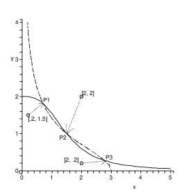
Figure 1: nullclines of system (9). (The dash line represents $f_{1}(x,y)=0$ and the solid one represents $f_{2}(x,y)=0$). The central equilibrium $P2$ can be shown to be unstable while the two others, $P1$ and $P3$ are stable. The arrows represent the three experimentations described in the text.

Applying our program in Maple, we found three different initial conditions each of which tends towards one of the three equilibrium points (see figure 1 and numerical results below). The convergence appears to be fast since we need only 4 iterations to approach the equilibria with a precision of $10^{-5}$. We will discuss about the convergence speed in part 5.1.

• With initial condition $x^{0}=(2,2)$, algorithm finished in 4 iterations and found $P2$ with a precision of $10^{-5}$. The numerical S-system obtained is given by:

  $$\left\{\begin{array}[]{lll}\dot{x}&=&1.500\,y^{-1}-x\\ \dot{y}&=&1.837\,x^{-1.5}-y\end{array}\right.$$

• With initial condition $x^{0}=(0.2,1.5)$, algorithm finished in 4 iterations and found $P1$ with a precision of $10^{-5}$. The numerical S-system obtained is given by:

  $$\left\{\begin{array}[]{lll}\dot{x}&=&1.745\,y^{-1.535}-x\\ \dot{y}&=&1.647\,x^{-0.274}-y\end{array}\right.$$

• With initial condition $x^{0}=(2,0.2)$, algorithm finished in 4 iterations and found $P3$ with a precision of $10^{-5}$. The numerical S-system obtained is given by:

  $$\left\{\begin{array}[]{lll}\dot{x}&=&2.352\,y^{-0.132}-x\\ \dot{y}&=&3.879\,x^{-2.6}-y\end{array}\right.$$

3.5 Stability analysis of approximate S-systems

Consider the $n$-dimensional dynamical system:

$$\left\{\begin{array}[]{l}\displaystyle\frac{dx}{dt}=F(x)=V^{+}(x)-V^{-}(x)\\ x\in{(\mathbb{R}^{*}_{+})^{n}}\end{array}\right.$$ (10)

Algorithm 1 ensures that, given any initial condition $x^{0}$ in ${(\mathbb{R}^{*}_{+})^{n}}$, unless we fall in a degenerate case, we produce a sequence $(x^{q})_{q\in\mathbb{N}}$ (with $x^{q}\in{(\mathbb{R}^{*}_{+})^{n}}$) that tends towards a limit point $\widetilde{x}\in{(\mathbb{R}^{*}_{+})^{n}}$ which is an equilibrium of (10). More precisely, $x^{q}=\Psi^{(q)}(x^{0})$.
Meanwhile, at each step, it provides us with a S-system $S_{q}(\alpha_{q},\beta_{q},G_{q},H_{q})$ which comes from the S-approximations of functions $V^{+}$ and $V^{-}$ in $x^{q}$. Thus, we have:

$$\left\{\begin{array}[]{lll}\alpha_{q}&=&\alpha(x^{q})\\ \beta_{q}&=&\beta(x^{q})\\ G_{q}&=&\displaystyle\left(g_{ij}^{q}\right)_{i,j=1\dots n}\text{ with: }g_{ij}^{q}=g_{ij}(x^{q})\\ H_{q}&=&\displaystyle\left(h_{ij}^{q}\right)_{i,j=1\dots n}\text{ with: }h_{ij}^{q}=h_{ij}(x^{q})\\ \end{array}\right.$$

where $\alpha$, $\beta$, $g_{ij}$ and $h_{ij}$ are the functions defined in (5). If we assume that $V^{+}$ and $V^{-}$ are at least $\mathcal{C}^{1}$, we deduce that these sequences converge, as $q$ tends to $\infty$, towards:

$$\left\{\begin{array}[]{lllll}\alpha_{q}&\rightarrow&\alpha(\widetilde{x})&\stackrel{{\scriptstyle def}}{{=}}&\widetilde{\alpha}\\ \beta_{q}&\rightarrow&\beta(\widetilde{x})&\stackrel{{\scriptstyle def}}{{=}}&\widetilde{\beta}\\ G_{q}&\rightarrow&G(\widetilde{x})&\stackrel{{\scriptstyle def}}{{=}}&\widetilde{G}\\ H_{q}&\rightarrow&H(\widetilde{x})&\stackrel{{\scriptstyle def}}{{=}}&\widetilde{H}\\ \end{array}\right.$$

Let $(\widetilde{S})$ be the following S-system:

$$(\widetilde{S})\,:\;\dot{x_{i}}=\widetilde{\alpha}_{i}\prod_{j=1}^{n}x_{j}^{\tilde{g}_{ij}}-\widetilde{\beta}_{i}\prod_{j=1}^{n}x_{j}^{\tilde{h}_{ij}},\;i=1\dots n$$ (11)

We want to know in what sense the system (11) approach the system (10). An answer is given by the following proposition:

Proposition 3.2

$F$ is supposed $\mathcal{C}^{r}$ ($r\geq 1$). The equilibrium $\widetilde{x}$ of (10) is an equilibrium of (11). Moreover, if $\widetilde{x}$ is hyperbolic, then the flow generated by (11) is topologically conjugate to the flow generated by (10) in a neighborhood of $\widetilde{x}$.

proof.
The first assertion is obvious with proposition 3.1. Let prove the second assertion: it is a direct consequence of the Hartman-Grobman theorem (see for instance [18]).
Proposition 3.1 shows that systems (10) and (11) have the same linearized dynamical systems in $\widetilde{x}$. Thanks to the Hartman-Grobman theorem, we know that these systems are topologically conjugate to their linearized dynamical systems. By transitivity of the topological conjugation, we deduce that (10) and (11) are topologically conjugate around $\widetilde{x}$.

$\Box$

This proposition implies that the stability of $\widetilde{x}$ for system (11) is the same that the stability of $\widetilde{x}$ for system (10). As an exemple, let us consider the following 2-dimensional dynamical system:

$$(Ex)\left\{\begin{array}[]{lll}\dot{x}&=&\displaystyle\frac{x}{2+y}-\frac{x^{2}y^{4}}{(3+x)(4+y^{3})}\\[8.53581pt] {}\dot{y}&=&\displaystyle\frac{5x}{3+x}-\frac{2xy^{3}}{(x+1)(y+2)}\\ \end{array}\right.$$

We find the equilibrium point $\widetilde{x}\approx(1.2301,1.6950)$ and the matrix $\widetilde{G}-\widetilde{H}$:

$$\widetilde{G}-\widetilde{H}=\left(\begin{array}[]{cc}-0.709&-2.812\\ 0.261&-2.541\end{array}\right)$$

Thanks to theorem 2.1, we see that $\widetilde{G}-\widetilde{H}$ is sign semi-stable. The point $\widetilde{x}$, as equilibrium of $(Ex)$ is hence stable.

4 Application to a biological example

We present here a current work we are doing in collaboration with G. Curien (see [4]). The goal of this work is to understand the metabolic system responsible for the synthesis of aminoacids in Arabidopsis Thaliana. So far, we have focused our study on a subsystem of $14$ variables, with $9$ symbolic parameters. The differential equations present several strongly nonlinear terms due to allosteric control of some enzymes ; in particular, Hill functions and compositions of Hill functions. Since the latter are rational functions, seeking positive equilibria is equivalent to solving a polynomial system. Algebraic manipulations have led us to a simplified system with $5$ polynomial equations in $5$ variables. Because of the complexity of these equations, we were not able to achieve the resolution of this system with purely symbolic computations and manipulating symbolic parameters (we used Maple 8 and 9). That is why symbolic-numeric methods appeared as a satisfactory way to tackle this problem. As it is a system of equations coming from biochemical kinetics, S-systems seemed to be an appropriate tool in this work.
In vivo, this system exhibits a stationnary behavior. Giving realistic values of parameters, we managed, thanks to our algorithm, to find this positive equilibrium. We now have to study the S-approximation of the system near this equilibrium, with different realistic sets of parameters. An interesting idea is also to propose a piecewise S-approximation of the system in order to reproduce its behavior in a wider zone of the phase space. This work is in progress.

5 Discussions and concluding remarks

5.1 Convergence of our algorithm

The algorithm described above computes the iterations of a vectorial function $\Psi$ on an initial point $x^{0}\in{(\mathbb{R}^{*}_{+})^{n}}$, in order to converge towards a fixed point of $\Psi$. As the jacobian of $\Psi$ is the null matrix in those fixed points, we know that the convergence speed is very fast (up to four or five iterations in all the examples presented, for a precision of $10^{-4}$ or $10^{-5}$). As a matter of fact, we are in a case where the speed of convergence is the best possible. Indeed, if the function $\Psi$ is $K$-contractant, one can easily verify that the convergence of the iteration is in $K^{n}$ (where $n$ is the number of iterations). Since $J_{\Psi}(\widetilde{x})=0$, then we can find a neighborhood of $\widetilde{x}$ wherein $\Psi$ is $K$-contractant for any $0<K<1$.
However, even if the speed of convergence is very fast, the algorithm behaviour is strongly dependent on the choice of initial point $x^{0}$. Indeed, if initial system has multiple positive equilibria, each of them have distinct basins of attraction. We cannot a priori know in which of these basins is the point $x^{0}$. We even cannot ensure that $x^{0}$ actually lye in one of them. In fact, the study of basins of attractions of such iterations is a complex issue. The boundaries of such basins can be quite complicated, even fractals [8]. As an example, we launched our algorithm for the switch system (equations (9)) with initial conditions taken on a grid of $]0,4]^{2}$. To vizualize the three basins, we colored the initial points (fig 2).

5.2 interaction between symbolic and numerical calculus

As we said in the introduction, a large part of research concerning the analysis of biological phenomena uses both symbolic and numerical techniques. The S-systems as we described represent a large class of systems, yet their simple mathematical expression allows symbolic manipulations, providing a practical framework of study. Algorithm 1, as presented here needs numerical estimations of symbolic parameters. Nevertheless the technique of S-approximation (def 3.1) consists of symbolic manipulations (in particular, we use symbolic computation of partial derivatives). It can be calculated in any point of the phase space and can include symbolic parameters.
S-approximation gives a computable and rather good approximation of ODE systems (see [17] for a comparison between power-law approximation and linearization). A very interesting idea is therefore to use the context information (given for instance by biologists) of a particular system in order to create a piecewise S-approximation of this system. This should provide a global approximation interpolating the system in some critical points in the phase space (see [13]).

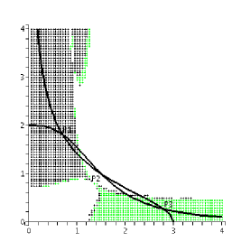
Figure 2: Basins of attraction of points $P1$ (dark), $P2$ (white) and $P3$ (grey). We obtained these graphs by applying algorithm 1 for system (9) with initial conditions taken in a regular grid of $]0,4]$.

References

- [1] M. Antoniotti, A. Policriti, N. Ugel, and B. Mishra. Xs-systems : extended s-systems and algebraic differential automata for modeling cellular behavior. Proceedings of the International Conference on Hih Performance Computing, HiPC 2002, pages 431–442, 2002.
- [2] L. Brenig and A. Goriely. Universal canonical forms for time continuous dynamical systems. Phys. Rev. A, 40:4119–4121, 1989.
- [3] J.L. Cherry and F.R. Adler. How to make a biological switch. J. Theor. Biol., 203:117–133, 2000.
- [4] G. Curien, S. Ravanel, and R. Dumas. A kinetic model of the branch-point between the methionine and threonine biosynthesis pathways in arabidopsis thaliana. Eur. J. Biochem., 270(23):4615–4627, 2003.
- [5] H. de Jong, J.-L. Gouz , C. Hernandez, M. Page, S. Tewfik, and J. Geiselmann. Qualitative simulation of genetic regulatory networks using piecewise-linear model. Bull. Math. Biol., 66(2):301–340, 2004.
- [6] L. Glass. Combinatorial and topological methods is nonlinear chemical kinetics. J. Chem. Phys., 63, 1975.
- [7] A. Goldbeter. Biochemical oscillations and cellular rhythms. Cambridge University Press, 1996.
- [8] C. Grebogi and E. Ott. Fractal basin boundaries, long-lived chaotic transients, and unstable-unstable pair bifurcation. Phys. Rev. Lett., 50(13):935–938, 1983.
- [9] C. Jeffries, V. Klee, and P. Van Den Driessche. When is a matrix sign stable ? Can. J. Math., 29(2):315–326, 1976.
- [10] R. Laubenbacher. A computer algebra approach to biological systems. Proceedings of the 2003 International Symposium on Symbolic and Algebraic Computation (ISSAC), 2003.
- [11] J. Maybee and J. Quirk. Qualitative problems in matrix theory. SIAM Review, 11(1):30–51, 1969.
- [12] T. Mestl, E. Plahte, and S.W. Omholt. A mathematical framework for describing and analyzing gene regulatory networks. J. Theor. Biol., 176:291–300, 1995.
- [13] M.A. Savageau. Alternative designs for a genetic switch: analysis of switching times using the piecewise power-law representation. Math. Biosci., 180:237–253, 2002.
- [14] M.A. Savageau and E.O. Voit. Recasting nonlinear differential equations as s-systems : a canonical nonlinear form. Math. Biosci., 87:83–115, 1987.
- [15] R. Thomas and M. Kaufman. Multistationarity, the basis of cell differentiation and memory. i. structural conditions of multistationarity and other non-trivial behaviour, and ii. logical analysis of regulatory networks in terms of feedback circuits. Chaos, 11:170–195, 2001.
- [16] E.O. Voit. Computational analysis of biochemical systems. Cambridge University Press, 2000.
- [17] E.O. Voit and M.A. Savageau. Accuracy of alternative representations for integrated biochemical systems. Biochemistry, 26:6869–6880, 1987.
- [18] S. Wiggins. Introduction to applied nonlinear dynamical systems and chaos. Springer Verlag, 1990.