Towards a divergence-free wavelet method for the simulation of 2D/3D turbulent flows

Abstract

In this paper, we investigate the use of compactly supported divergence-free wavelets for the representation of the Navier-Stokes solution. After reminding the theoretical construction of divergence-free wavelet vectors, we present in detail the bases and corresponding fast algorithms for 2D and 3D incompressible flows. In order to compute the nonlinear term, we propose a new method which provides in practice with the Hodge decomposition of any flow: this decomposition enables us to separate the incompressible part of the flow from its orthogonal complement, which corresponds to the gradient component of the flow. Finally we show numerical tests to validate our approach.

1 Introduction

The prediction of fully-developed turbulent flows represents an extremely challenging field of research in scientific computing. The Direct Numerical Simulations (DNS) of turbulence requires the integration in time of the nonlinear Navier-Stokes equations, which assumes the computation of all scales of motion. However, at large Reynolds number, turbulent flows generate increasingly small scales: to be realistic, the discretization in space (and correlatively in time) ought to handle a huge number of degrees of freedom, that is in 3D out of the reach of available computers.

Many tentatives have been done or are underway to overcome this problem: one can cite the Vortex Methods which are able to generate very thin scales, or Large Eddy Simulation (LES) and subgrid-scale techniques which separate the flow into large scales, that are explicitly computed, from the small scales, that are parametrized or statistically computed.

In that context, wavelet bases offer an intermediate decomposition to suitably represent the intermittent spatial structure of turbulent flows, with only few degrees of freedom: this property is mainly due to the good localization, both in physical and frequency domains, of the basis functions. The wavelet decomposition was introduced in the beginning of the 90s for the analysis of turbulent flows [8, 23, 21]. Wavelet based methods for the resolution of the Navier-Stokes equations appear later [2, 11, 9, 16, 13]. They have also been used to define LES-type methods such as the CVS method [10]. Most of the works cited below use a Galerkin or a Petrov-Galerkin approach for the 2D vorticity formulation with periodic boundary conditions. However, if we want to turn to the 3D case, with non periodic boundary conditions, these approaches are no more available.

An alternative was at the same period firstly considered by K. Urban and after investigated by several authors: they proposed to use the divergence-free wavelet bases originally designed by Lemarié-Rieusset [19]. Divergence-free wavelet vectors have been implemented and used to analyze 2D turbulence flows [1, 15, 29], as well as to compute the 2D/3D Stokes solution for the driven cavity problem [26, 27]. Seeing that divergence-free wavelets are constructed from standard compactly supported biorthogonal wavelet bases, they allow to incorporate boundary conditions in their construction [5, 28].

This research direction is of great interest, since divergence-free wavelets provide with bases suitable to represent the incompressible Navier-Stokes solution, in two and three dimension. Our objective is now to investigate their feasibility and amenability for such problem. The first point lies in avoiding the pressure by projecting the equations onto the space of divergence-free vectors. This (orthogonal) projection is the well-known Leray projector, and it can be computed explicitly in Fourier space, for periodic boundary conditions. Unfortunately, as already noted by K. Urban [28], if we want to explicit the Leray operator in terms of divergence-free wavelets, since they form biorthogonal bases (and not orthogonal), they would not give rise, in a simple way, to the orthogonal projection onto the space of divergence-free vectors.

Nevertheless, we propose in the present paper to investigate the use of divergence-free wavelets for the simulation of turbulent flows. Firstly, we remind the basic ingredients of the theory of compactly supported divergence-free wavelet vectors, developed by Lemarié-Rieusset [19]. In section 3, we present in detail the bases we proposed to implement in space dimensions 2 and 3. We will see that the choice of the complement wavelet basis is not unique from this construction, and it induces the values of divergence-free coefficients, for compressible flows. We discuss the algorithmic implementation of divergence-free wavelet coefficients in dimensions 2 and 3, leading to fast algorithms (in O($N$) operations where $N$ is the number of grid points).

Section 4 is devoted to the Hodge decomposition of a compressible field, in a wavelet formulation: the method we present uses both the biorthogonal projectors on divergence-free, and on curl-free wavelets: our method is an iterative procedure, and we will experimentally prove that it converges. The last section presents numerical tests to validate our approach: nonlinear compression of 2D and 3D incompressible turbulent flows, and Hodge decomposition of well chosen examples, such as the nonlinear term of the Navier-Stokes equations.

2 Theory of divergence-free wavelet bases

In this section, we review briefly the relevant properties of wavelet bases, that will be used for the construction of divergence-free wavelets. Compactly supported divergence-free vector wavelets were originally designed by Lemarié-Rieusset, in the context of biorthogonal Multiresolution Analyses. We illustrate the construction with the explicit example of splines of degree 1 and 2. For more details, we refer to [19, 6, 17, 27].

2.1 Multiresolution Analyses (MRA)

Multiresolution Analyses (MRA) are approximation spaces allowing the construction of wavelet bases, introduced by S. Mallat [22]. We begin with the one-dimensional case of functions defined on the real line.

Definition (MRA): A Multiresolution Analysis of $L^{2}(\mathbb{R})$ is a sequence of closed subspaces $(V_{j})_{j\in\mathbb{Z}}$ verifying:

(1)

$\forall j,~{}~{}V_{j}\subset V_{j+1},\quad\bigcap_{j\in\mathbb{Z}}V_{j}=\{0\},\quad\bigcup_{j\in\mathbb{Z}}V_{j}\mbox{ is dense in }L^{2}(\mathbb{R})$

(2)

(Dilation invariance)  $f\in V_{j}\quad\iff\quad f(2.)\in V_{j+1}$

(3)

(Shift-invariance)  There exists a function $\phi\in V_{0}$ such that the family $\{\phi(.-k)~{};~{}k\in\mathbb{Z}\}$ form a (Riesz) basis of $V_{0}$.

The function $\phi$ in (3) is called a scaling function of the MRA.
Here, $j$ denotes the level of refinement. By virtue of the dilation invariance property (2) above, we can deduce that each space $V_{j}$ is spanned by $\{\phi_{j,k}~{};~{}k\in\mbox{$\mathbb{Z}$}\}$ where $\phi_{j,k}(x)=2^{j/2}\phi(2^{j}x-k)$.

Wavelets appear as bases of complementary spaces $W_{j}$:

$$V_{j+1}=V_{j}\oplus W_{j}$$ (1)

where the sum is direct, but not necessarily orthogonal. In this context (called the biorthogonal case), the choice of spaces $W_{j}$ is not unique. The problem of constructing the spaces $W_{j}$ means to find a function $\psi$, called wavelet such that the system $\{\psi(.-k)~{}~{};k\in\mathbb{Z}\}$ spans $W_{0}$. Repeated decomposition of $V_{j}$ yields the multiresolution analysis of $V_{j}$ with the wavelet spaces:

$$V_{j}=V_{0}\bigoplus_{\ell=0}^{j-1}W_{\ell}$$

which leads, when $j\to+\infty$, to the wavelet decomposition of the whole space:

$$L^{2}(\mathbb{R})=V_{0}\bigoplus_{\ell=0}^{+\infty}W_{\ell}$$

As a result, we can write any function $f\in L^{2}(\mathbb{R})$ in the basis $\{\phi_{k},~{}\psi_{j,k}~{};~{}j\geq 0,k\in\mathbb{Z}\}$, with $\phi_{k}=\phi\cdot-k)$ and $\quad\psi_{j,k}=2^{j/2}\psi(2^{j}\cdot-k)$:

$$f=\sum_{k\in\mathbb{Z}}c_{k}~{}\mathbf{\phi}_{k}+\sum_{j\geq 0}\sum_{k\in\mathbb{Z}}~{}d_{j,k}~{}\mathbf{\psi}_{j,k}$$ (2)

Dual bases: Let a pair $(\phi,\psi)$ of scaling function and wavelet, arising from a Multiresolution Analysis, be given, then we can associate a unique dual pair $(\phi^{*},\psi^{*})$, such that the following biorthogonality (in space $L^{2}$) relations are fulfilled: for all $k\in\mathbb{Z}$ and $j\geq 0$,

$$<\phi|\phi^{*}_{k}>=\delta_{k,0},~{}<\phi|\psi^{*}_{j,k}>=0,~{}<\psi|\psi^{*}_{j,k}>=\delta_{j,0}\delta_{k,0},~{}<\psi|\phi^{*}_{k}>=0$$ (3)

Moreover the dual scaling functions $\phi^{*}_{k}$ and the dual wavelets $\psi^{*}_{j,k}$ have the same structure as above: $\phi^{*}_{k}=\phi^{*}(\cdot-k)$ and $\psi^{*}_{j,k}=2^{j/2}\psi^{*}(2^{j}\cdot-k)$.

Scaling equations and filter design: Since the function $\frac{1}{\sqrt{2}}\phi(\frac{\cdot}{2})$ lives in $V_{0}$, there exists a sequence $(h_{k})$ (also called the low pass filter) verifying:

$$\frac{1}{\sqrt{2}}\phi(\frac{x}{2})=\sum_{k\in\mathbb{Z}}h_{k}~{}\phi(x-k)$$ (4)

By applying the Fourier transform, (4) rewrites:

$$\hat{\phi}(2\xi)=m_{0}(\xi)\hat{\phi}(\xi)$$

where $m_{0}(\xi)=\frac{1}{\sqrt{2}}\sum_{k\in\mathbb{Z}}h_{k}e^{-ik\xi}$ is the transfer function of the filter $(h_{k})$.

Again, because of $W_{-1}\subset V_{0}$, the wavelet satisfies a two-scale equation:

$$\frac{1}{\sqrt{2}}\psi(\frac{x}{2})=\sum_{k\in\mathbb{Z}}g_{k}~{}\phi(x-k)$$ (5)

where the coefficients $(g_{k})$ are called the high pass filter. Again the Fourier transform of $\psi$ expresses with the transfer function $n_{0}$ of filter $g_{k}$ as:

$$\hat{\psi}(2\xi)=n_{0}(\xi)\hat{\phi}(\xi)$$

In the same way, the dual functions satisfy scaling equations:

$$\begin{array}[]{ccc}\frac{1}{\sqrt{2}}\phi^{*}(\frac{x}{2})=\sum_{k\in\mathbb{Z}}h^{*}_{k}~{}\phi^{*}(x-k),&&\hat{\phi^{*}}(2\xi)=m^{*}_{0}(\xi)\hat{\phi^{*}}(\xi)\\ \frac{1}{\sqrt{2}}\psi^{*}(\frac{x}{2})=\sum_{k\in\mathbb{Z}}g^{*}_{k}~{}\phi^{*}(x-k),&&\hat{\psi^{*}}(2\xi)=n^{*}_{0}(\xi)\hat{\phi^{*}}(\xi)\end{array}$$ (6)

Following [17, 6], the biorthogonality conditions (3) for the scaling functions imply:

$$m_{0}(\xi)\overline{m^{*}_{0}(\xi)}+m_{0}(\xi+\pi)\overline{m^{*}_{0}(\xi+\pi)}=1\quad$$

while one can choose, for example, as transfer functions for the associated wavelets:

$$\begin{array}[]{ccc}n_{0}(\xi)=e^{-i\xi}~{}\overline{m^{*}_{0}(\xi+\pi)},&&n^{*}_{0}(\xi)=e^{-i\xi}~{}\overline{m_{0}(\xi+\pi)}\end{array}$$

which corresponds to:

$$g_{k}=(-1)^{1-k}~{}h^{*}_{1-k},~{}~{}~{}g^{*}_{k}=(-1)^{1-k}~{}h_{1-k},~{}~{}\forall k$$

In practice, the filter coefficients $h_{k}$ and $g_{k}$ are all what is needed to compute the wavelet decomposition (2) of a given function. Notice that these filters are finite if and only if the functions $\psi$ and $\phi$ are compactly supported.

Example: symmetric biorthogonal splines of degree 1
A simple example for spaces $V_{j}$ are the spaces of continuous functions, which are piecewise linear on the intervals $[k2^{-j},(k+1)2^{-j}]$, for $k\in\mbox{$\mathbb{Z}$}$. In this case we can choose as scaling function the hat function $\phi(x)=\max(0,1-|x|)$. Its transfer function is given by

$$m_{0}(\xi)=e^{i\xi}~{}\left(\frac{1+e^{-i\xi}}{2}\right)^{2}$$ (7)

The shortest even dual scaling function associated with $\phi$ is associated with the filter:

$$m^{*}_{0}(\xi)=e^{i\xi}~{}\left(\frac{1+e^{-i\xi}}{2}\right)^{2}(2-\cos\xi)$$ (8)

The corresponding values of filters $(h_{k})$ and $(h^{*}_{k})$ are given in table 1. Figure 1 displays the scaling functions and their associated wavelets in this case.

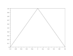
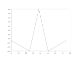
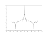
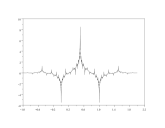
Figure 1: From left to right: the scaling function $\phi$ with its associated symmetric wavelet with shortest support, and their duals: the dual scaling function $\phi^{*}$ and the dual wavelet $\psi^{*}$.

2.2 Decomposition-recomposition algorithm and useful example

In the context of a biorthogonal Multiresolution Analysis, the wavelet decomposition of a given function $f\in L^{2}(\mbox{\mat{R}})$ (equation (2)), is obtained through the now well known Fast Wavelet Transform [22]. We briefly review here the formula that will be useful for the following.

In practice we begin with an approximation $f_{J}$ of $f$ in some space $V_{J}$ of the MRA. This approximation may be the oblique projection of $f$ onto $V_{J}$ following the direction perpendicular to $V^{*}_{J}$ (also called the biorthogonal projection on $V_{J}$); but usually $f_{J}$ means an interpolating function of $f$, associated to nodes $\{k2^{-J}~{};~{}k\in\mbox{$\mathbb{Z}$}\}$ (see in last section some examples of procedure).

This approximation $f_{J}$ of function $f$ may be expanded in terms of the scaling basis $\phi_{J,k}=2^{J/2}\phi(2^{J}x-k)$ of $V_{J}$:

$$f_{J}(x)=2^{J/2}\sum_{k=-\infty}^{+\infty}c_{J,k}~{}\phi(2^{J}x-k)$$

The wavelet decomposition of $f_{J}$ corresponds to a truncated sum in equation (2) up to the level $J-1$, meaning that $2^{-J}$ is the finest scale of approximation:

$$f_{J}=\sum_{k\in\mathbb{Z}}c_{k}~{}\mathbf{\phi}_{k}+\sum_{j=0}^{J-1}\sum_{k\in\mathbb{Z}}~{}d_{j,k}~{}\mathbf{\psi}_{j,k}$$ (9)

The wavelet coefficients $d_{j,k}$ are then computed recursively on the level $j$, from $j=J-1$ to $j=1$ using the decomposition of spaces (1):

$$f_{j+1}=\sum_{k=-\infty}^{+\infty}c_{j+1,k}~{}\phi_{j+1,k}=\sum_{k=-\infty}^{+\infty}c_{j,k}~{}\phi_{j,k}+\sum_{k=-\infty}^{+\infty}d_{j,k}~{}\psi_{j,k}$$

(Here $f_{j+1}$ denotes the biorthogonal projection of $f_{J}$ onto $V_{j+1}$). By biorthogonality (3) one has:

$$c_{j,k}=<f_{j+1}|\phi^{*}_{j,k}>~{},~{}~{}d_{j,k}=<f_{j+1}|\psi^{*}_{j,k}>~{},~{}~{}c_{j+1,k}=<f_{j+1}|\phi^{*}_{j+1,k}>$$

which yield the decomposition formula: for all $j=0,\dots J-1$,

$$\left\{\begin{array}[]{c}c_{j,k}=\sum_{\ell}h^{*}_{\ell}~{}c_{j+1,\ell+2k}\\ \vspace{0.1cm}\hfil\\ d_{j,k}=\sum_{\ell}g^{*}_{\ell}~{}c_{j+1,\ell+2k}\end{array}\right.$$

where the filters $h^{*}_{\ell}$ and $g^{*}_{\ell}$ arise from the scaling equations (6) of the dual basis functions.
In the same way, we obtain the reconstruction formula:

$$c_{j+1,k}=\sum_{\ell}\left(h_{k-2\ell}~{}c_{j,\ell}+g_{k-2\ell}~{}d_{j,\ell}\right)$$

where $h_{k}$ and $g_{k}$ are the filters provided by the scaling equations (4, 5) of the primal basis functions.

The computing cost for the whole wavelet decomposition (9) (as well as for the recomposition) is about $C2^{J}$ operations, where $2^{J}$ is the number of point values $f(k2^{-J})$ we start with, and $C$ means the length of the filters ($h^{*}_{k}$ for the decomposition, $h_{k}$ for the synthesis).

Example: spline wavelets of degree 1 and 2: Biorthogonal splines provide with wavelet bases which are regular, compactly-supported and easy to implement. The scaling functions of the associated MRA are standard B-spline bases, and the wavelets are constructed easily, by linear combinations of translated B-splines. We focus here on two examples of wavelet bases, which will be useful for the construction of divergence-free wavelets: splines of degree 1 ($V^{0}_{j}$ MRA spaces) and splines of degree 2 ($V^{1}_{j}$ MRA spaces). In both cases we draw the scaling functions and the associated wavelets with shortest support (figure 2).

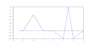
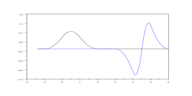
$\phi_{0}\qquad\qquad\qquad\psi_{0}$	$\phi_{1}\qquad\qquad\qquad\psi_{1}$

Figure 2: Scaling functions and associated even and odd wavelets with shortest support, for splines of degree 1 (left) and 2 (right).

In both cases the filters are easy to compute (see [17, 6]). Since the support of basis function is very short, the filters have a few non zero coefficients. The values of the decomposition and reconstruction filters are given on Table 1.

$$\begin{array}[]{|c|c|c|c|c|c|c|}\hline\cr\ell&-2&-1&0&1&2&3\\ \hline\cr\frac{1}{\sqrt{2}}h^{*0}_{\ell}&-1/8&1/4&3/4&1/4&-1/8&0\\ \hline\cr\frac{1}{\sqrt{2}}g^{*0}_{\ell}&0&0&-1/4&1/2&-1/4&0\\ \hline\cr\frac{1}{\sqrt{2}}h_{\ell}^{0}&0&1/4&1/2&1/4&0&0\\ \hline\cr\frac{1}{\sqrt{2}}g_{\ell}^{0}&0&-1/8&-1/4&3/4&-1/4&-1/8\\ \hline\cr\end{array}~{}~{}~{}~{}~{}~{}\begin{array}[]{|c|c|c|c|c|}\hline\cr\ell&-1&0&1&2\\ \hline\cr\frac{1}{\sqrt{2}}h^{*1}_{\ell}&-1/4&3/4&3/4&-1/4\\ \hline\cr\frac{1}{\sqrt{2}}g^{*1}_{\ell}&1/8&-3/8&3/8&-1/8\\ \hline\cr\frac{1}{\sqrt{2}}h_{l}^{1}&1/8&3/8&3/8&1/8\\ \hline\cr\frac{1}{\sqrt{2}}g_{l}^{1}&-1/4&-3/4&3/4&1/4\\ \hline\cr\end{array}$$

Table 1: Decomposition filter ($h^{*}_{k},~{}g^{*}_{k}$) and reconstruction filter ($h_{k},~{}g_{k}$) coefficients, associated to piecewise linear splines (left) and piecewise quadratic splines (right), verifying (11) (see hereafter) with shortest supports.

2.3 Multivariate wavelets

The above considerations can be extended to multi-D. The simplest way to obtain multivariate wavelets is to employ anisotropic or isotropic tensor products of one-dimensional functions.
To be more precise, we focus on the two dimensional case: let $(V^{0}_{j})$ and $(V^{1}_{j})$ two multiresolution analyses of $L^{2}(\mbox{\mat{R}})$ be given, associated with scaling functions and wavelets $(\phi_{0},\psi_{0})$ and $(\phi_{1},\psi_{1})$; the two dimensional tensor product space $V^{0}_{J}\otimes V^{1}_{J}$ is generated by the scaling basis $\{\phi_{0,J,k_{1}}(x)\phi_{1,J,k_{2}}(y);(k_{1},k_{2})\in\mbox{$\mathbb{Z}$}^{2}\}$, where $\phi_{0,J,k_{1}}(x)=2^{J/2}\phi_{0}(2^{J}x-k_{1})$ and similarly for $\phi_{1,J,k_{2}}$. Then each function $f_{J}$ in $V^{0}_{J}\otimes V^{1}_{J}$ can be written:

$$f_{J}(x,y)=\sum_{k_{1}=-\infty}^{\infty}\sum_{k_{2}=-\infty}^{\infty}c_{J,k_{1},k_{2}}~{}2^{J}\phi_{0}(2^{J}x-k_{1})~{}\phi_{1}(2^{J}y-k_{2})$$ (10)

The anisotropic 2D wavelets are constructed with tensor products of wavelets at different scales $\{\psi_{0,j_{1},k_{1}}(x)\psi_{1,j_{2},k_{2}}(y)\}$. For certain choices of $j_{1},j_{2}$, the support of the functions may be very lengthened. In this case the wavelet decomposition of $f_{J}$ writes:

$$f_{J}(x,y) = \sum_{(k_{1},k_{2})\in\mbox{$\mathbb{Z}$}^{2}}c_{k_{1},k_{2}}~{}\phi_{0}(x-k_{1})~{}\phi_{1}(y-k_{2})$$

$$+\sum_{j_{1}=0}^{J-1}\sum_{j_{2}=0}^{J-1}2^{(j_{1}+j_{2})/2}\sum_{(k_{1},k_{2})\in\mbox{$\mathbb{Z}$}^{2}}d_{j_{1},j_{2},k_{1},k_{2}}~{}\psi_{0}(2^{j_{1}}x-k_{1})~{}\psi_{1}(2^{j_{2}}y-k_{2})$$

The anisotropic decomposition is the most easy way to compute a multi-dimensional wavelet transform, as it corresponds to apply one-dimensional wavelet decompositions in each direction. In the 2D case, this is schematized in figure 3.

Figure 3: Anisotropic 2D wavelet transform.

In the isotropic case, the 2D wavelets are obtained through tensor products of wavelets and scaling functions or wavelets at the same scale. This produces the following decomposition for $f_{J}$:

$$f_{J}(x,y) = \sum_{(k_{1},k_{2})\in\mbox{$\mathbb{Z}$}^{2}}c_{k_{1},k_{2}}~{}\phi_{0}(x-k_{1})~{}\phi_{1}(y-k_{2})$$

$$+\sum_{j_{=}0}^{J-1}\left(\sum_{k_{1},k_{2}}d_{j,k_{1},k_{2}}^{(1,0)}~{}\psi_{0,j,k_{1}}(x)~{}\phi_{1,j,k_{2}}(y)+\sum_{k_{1},k_{2}}d_{j,k_{1},k_{2}}^{(1,1)}~{}\psi_{0,j,k_{1}}(x)~{}\psi_{1,j,k_{2}}(y)\right.$$

$$\left.\quad+\sum_{k_{1},k_{2}}d_{j,k_{1},k_{2}}^{(0,1)}~{}\phi_{0,j,k_{1}}(x)~{}\psi_{1,j,k_{2}}(y)\right)$$

As one can see, this decomposition involves three kinds of wavelets, one following the direction $x$: $\Psi^{(1,0)}(x,y)=\psi_{0}(x)~{}\phi_{1}(y)$, one following the direction $y$: $\Psi^{(0,1)}(x,y)=\phi_{0}(x)~{}\psi_{1}(y)$ and one in both directions: $\Psi^{(1,1)}(x,y)=\psi_{0}(x)~{}\psi_{1}(y)$. The interest of this basis remains in the fact that the size of their support is proportional to $2^{-j}$ in each direction, i.e. the basis functions are rather isotropic. The principle of the associated decomposition algorithm is illustrated by figure 4.

Figure 4: Isotropic 2D wavelet transform.

2.4 Theoretical ground of the divergence-free wavelet vectors

Let introduce

$$\vec{\textbf{H}}_{\textrm{div}}(\mbox{\mat{R}}^{n})=\{f\in(L^{2}(\mathbb{R}^{n}))^{n}/\textrm{div}f\in L^{2}(\mathbb{R}^{n}),\quad\textrm{div}f=0\}$$

the space of divergence-free vector functions in $\mbox{\mat{R}}^{n}$.
The construction of compactly divergence-free wavelets in $(L^{2}(\mathbb{R}^{n}))^{n}$, which will correspond to Riesz bases of $\vec{\textbf{H}}_{\textrm{div}}(\mbox{\mat{R}}^{n})$, was originally derived by Lemarié-Rieusset [19]: it is based on the following proposition, which relates two different multiresolution analyses of $L^{2}(\mathbb{R})$ by differentiation and integration:

Proposition: Let $(V^{0}_{j})$ a one-dimensional MRA with a derivable scaling function $\phi_{1}$ and a wavelet $\psi_{1}$, be given. Then, we can build a MRA $(V^{1}_{j})$ with a scaling function $\phi_{0}$ and a wavelet $\psi_{0}$ verifying:

$$V_{0}^{0}=\textrm{span}\{\phi_{0}(x-k),k\in\mbox{$\mathbb{Z}$}\}\qquad V_{0}^{1}=\textrm{span}\{\phi_{1}(x-k),k\in\mbox{$\mathbb{Z}$}\}$$

and

$$\phi_{1}^{\prime}(x)=\phi_{0}(x)-\phi_{0}(x-1)\qquad\psi_{1}^{\prime}(x)=4~{}\psi_{0}(x)$$ (11)

For the refinement polynomials it can be traduced by:

$$m_{0}(\xi)=\frac{2}{1+e^{-i\xi}}~{}m_{1}(\xi)$$

Equation (11) rewrites for the dual functions $\phi_{0}^{*}$, $\psi_{0}^{*}$, $\phi_{1}^{*}$, and $\psi_{1}^{*}$:

$${\phi_{0}^{*}}^{\prime}(x)=\phi_{1}^{*}(x+1)-\phi_{1}^{*}(x)\\ {\psi_{0}^{*}}^{\prime}(x)=-4~{}\psi_{1}^{*}(x)$$ (12)

which induces:

$$m_{0}^{*}(\xi)=\frac{1+e^{i\xi}}{2}~{}m_{1}^{*}(\xi)$$

Example: As an example of functions fulfilling the above proposition, one shall cite the piecewise linear spline functions $\phi_{0}$, $\psi_{0}$, associated with the piecewise quadratic spline functions $\phi_{1}$, $\psi_{1}$ introduced in section 2.2, and plotted on figure 2.

Then, the divergence-free wavelets are explicitly constructed by combining suitable tensor products of these functions. For instance, in the 2D case we may have the following basis [19]:

Example: The 2D divergence-free vector scaling function takes the form:

$$\begin{array}[]{llll}\Phi_{\textrm{div}}(x_{1},x_{2})=\left|\begin{array}[]{l}\phi_{1}(x_{1}){\phi_{1}}^{\prime}(x_{2})\\ -{\phi_{1}}^{\prime}(x_{1})\phi_{1}(x_{2})\end{array}\right.&=&\left|\begin{array}[]{l}\phi_{1}(x_{1})~{}[\phi_{0}(x_{2})-\phi_{0}(x_{2}-1)]\\ -[\phi_{0}(x_{1})-\phi_{0}(x_{1}-1)]~{}\phi_{1}(x_{2})\end{array}\right.\end{array}$$

and the corresponding isotropic vector wavelets are given by the system:

$$\begin{array}[]{ll}\Psi_{\textrm{div}}^{(1,0)}(x_{1},x_{2})=\left|\begin{array}[]{l}-\frac{1}{4}\psi_{1}(x_{1})[\phi_{0}(x_{2})-\phi_{0}(x_{2}-1)]\\ \psi_{0}(x_{1})\phi_{1}(x_{2})\end{array}\right.\\ \vspace{1mm}&\vspace{1mm}\\ \Psi_{\textrm{div}}^{(0,1)}(x_{1},x_{2})=\left|\begin{array}[]{l}\phi_{1}(x_{1})\psi_{0}(x_{2})\\ -\frac{1}{4}[\phi_{0}(x_{1})-\phi_{0}(x_{1}-1)]\psi_{1}(x_{2})\end{array}\right.\\ \vspace{1mm}&\vspace{1mm}\\ \Psi_{\textrm{div}}^{(1,1)}(x_{1},x_{2})=\left|\begin{array}[]{l}\psi_{1}(x_{1})\psi_{0}(x_{2})\\ -\psi_{0}(x_{1})\psi_{1}(x_{2})\end{array}\right.\end{array}$$

It can be easily seen that the dilated and translated functions $\Psi_{\textrm{div},j,\mbox{$\mathbf{k}$}}^{\varepsilon}=2^{j}\Psi_{\textrm{div}}^{\varepsilon}(2^{j}x_{1}-k_{1},2^{j}x_{2}-k_{2})$ with $j,k_{1},k_{2}\in\mbox{$\mathbb{Z}$}$ and $\varepsilon\in\{0,1\}^{2}\setminus(0,0)$ span the space $\vec{\textbf{H}}_{\textrm{div}}(\mbox{\mat{R}}^{2})$ of divergence-free vector functions in $\mbox{\mat{R}}^{2}$. We represent in figure 5 the three generating functions in the case of spline generators of degree 1 and 2 of figure 2.

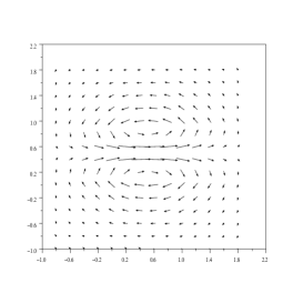
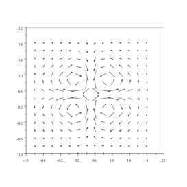
Figure 5: Isotropic 2D generating divergence-free wavelets $\Psi_{\textrm{div}}^{(1,0)}$ (left), $\Psi_{\textrm{div}}^{(0,1)}$ (center) and $\Psi_{\textrm{div}}^{(1,1)}$ (right).

More generally, the construction of divergence-free wavelets in $\mbox{\mat{R}}^{n}$ is carried out by suitable combinations of tensor products of functions $\phi_{0}$, $\psi_{0}$, and $\phi_{1}$, $\psi_{1}$, satisfying the above proposition (see [19, 27, 28]). These allow to state the following theorem of existence of isotropic divergence-free wavelet bases in the general case [19]:

Theorem: There exist $(n-1)(2^{n}-1)$ vector functions $\Psi_{\textrm{div},i}^{\varepsilon}\in\vec{\textbf{H}}_{\textrm{div}}(\mbox{\mat{R}}^{n})$ ($\varepsilon\in\Omega_{n}^{*}$ of cardinal $(2^{n}-1)$, $1\leq i\leq n-1$) compactly supported, such that every vector function $\mbox{$\mathbf{u}$}\in\vec{\textbf{H}}_{\textrm{div}}(\mbox{\mat{R}}^{n})$ can be expanded in a unique way:

$$\mbox{$\mathbf{u}$}=\sum_{j\in\mbox{$\mathbb{Z}$}}\sum_{\varepsilon\in\Omega_{n}^{*}}\sum_{\mbox{$\mathbf{k}$}\in\mbox{$\mathbb{Z}$}^{n}}d_{\mbox{div},i,j,\mbox{$\mathbf{k}$}}^{\varepsilon}~{}\Psi_{\textrm{div},i,j,\mbox{$\mathbf{k}$}}^{\varepsilon}$$

and one has, for a constant $C>0$ independent from $\mbox{$\mathbf{u}$}=(u_{1},u_{2},\dots,u_{n})$:

$$\frac{1}{C}\|\mbox{$\mathbf{u}$}\|_{\vec{L}^{2}}\leq\bigg{\{}\sum_{j\in\mbox{$\mathbb{Z}$}}\sum_{\varepsilon\in\Omega_{n}}\sum_{\mbox{$\mathbf{k}$}\in\mbox{$\mathbb{Z}$}^{n}}|d_{\mbox{div},i,j,\mbox{$\mathbf{k}$}}^{\varepsilon}|^{2}\bigg{\}}^{1/2}\leq C\|\mbox{$\mathbf{u}$}\|_{\vec{L}^{2}}$$

where $\|\mbox{$\mathbf{u}$}|_{\vec{L}^{2}}^{2}=\sum_{i=1}^{n}\|u_{i}\|_{L^{2}}^{2}$.

These wavelets have already been studied by several authors for 2D analyses of turbulent flows [1, 15], and also to solve the Stokes problem in two and three dimensions [26, 27, 28]. From now on, we will focus on the 2D and 3D case, and we will see that the expansion of compressible flow in terms of divergence-free wavelet bases is not uniquely given. We will also present in a practical way, the associated fast algorithms.

3 Practical implementation of divergence-free wavelets

In this section, we present in detail the two and three-dimensional divergence-free wavelet bases, and we study how to compute the associated fast wavelet transforms. We present the constructions in the isotropic multivariate wavelet case (see section 2.3), and also in the anisotropic one, which differs somewhat from previous studies.

In the following, we are given two 1D multiresolution analyses $(V^{0}_{j})$ and $(V^{1}_{j})$ satisfying the proposition of section 2.4. We note $\phi_{0}$, $\psi_{0}$ and $\phi_{1}$, $\psi_{1}$ their associated (one-dimensional) scaling functions and wavelets.

3.1 Isotropic divergence-free wavelet transforms

3.1.1 The 2D case

The starting point of the construction lies in considering as 2D multiresolution analysis of $L^{2}(\mbox{\mat{R}}^{2})^{2}$ the vector space of tensor-products $(V^{1}_{j}\otimes V^{0}_{j})\times(V^{0}_{j}\otimes V^{1}_{j})$. In the isotropic case, the 2D scaling functions $\Phi_{1}$, $\Phi_{2}$ and the 2D wavelets $\Psi_{1}^{\varepsilon}$, $\Psi_{2}^{\varepsilon}$ of this MRA are given by:

$$\begin{array}[]{llcll}\Phi_{1}(x_{1},x_{2})=&\left|\begin{array}[]{l}\phi_{1}(x_{1})\phi_{0}(x_{2})\\ 0\end{array}\right.&&\Phi_{2}(x_{1},x_{2})=&\left|\begin{array}[]{l}0\\ \phi_{0}(x_{1})\phi_{1}(x_{2})\end{array}\right.\\ \vspace{0.3mm}&\vspace{0.3mm}&\vspace{0.3mm}\hfil&\vspace{0.3mm}\\ \Psi_{1}^{(1,0)}(x_{1},x_{2})=&\left|\begin{array}[]{l}\psi_{1}(x_{1})\phi_{0}(x_{2})\\ 0\end{array}\right.&&\Psi_{2}^{(1,0)}(x_{1},x_{2})=&\left|\begin{array}[]{l}0\\ \psi_{0}(x_{1})\phi_{1}(x_{2})\end{array}\right.\\ \vspace{0.3mm}&\vspace{0.3mm}&\vspace{0.3mm}\hfil&\vspace{0.3mm}\\ \Psi_{1}^{(0,1)}(x_{1},x_{2})=&\left|\begin{array}[]{l}\phi_{1}(x_{1})\psi_{0}(x_{2})\\ 0\end{array}\right.&&\Psi_{2}^{(0,1)}(x_{1},x_{2})=&\left|\begin{array}[]{l}0\\ \phi_{0}(x_{1})\psi_{1}(x_{2})\end{array}\right.\\ \vspace{0.3mm}&\vspace{0.3mm}&\vspace{0.3mm}\hfil&\vspace{0.3mm}\\ \Psi_{1}^{(1,1)}(x_{1},x_{2})=&\left|\begin{array}[]{l}\psi_{1}(x_{1})\psi_{0}(x_{2})\\ 0\end{array}\right.&&\Psi_{2}^{(1,1)}(x_{1},x_{2})=&\left|\begin{array}[]{l}0\\ \psi_{0}(x_{1})\psi_{1}(x_{2})\end{array}\right.\end{array}$$

As explained in section 2.3, the functions

$$\bigg{\{}\Psi_{i,j,\mbox{$\mathbf{k}$}}^{\varepsilon}(x_{1},x_{2})=2^{j}\Psi_{i}^{\varepsilon}(2^{j}x_{1}-k_{1},2^{j}x_{2}-k_{2})\bigg{\}}\\$$

with $j\in\mbox{$\mathbb{Z}$},\mbox{$\mathbf{k}$}=(k_{1},k_{2})\in\mbox{$\mathbb{Z}$}^{2},\varepsilon\in\{(0,1),(1,0),(1,1)\},i=1,2$, form a basis of $(L^{2}(\mathbb{R}^{2}))^{2}$. Then, a velocity field $\mathbf{u}$ in $(L^{2}(\mathbb{R}^{2}))^{2}$ has the following wavelet decomposition:

$$\mathbf{u} =~{}\sum_{j\in\mbox{$\mathbb{Z}$}}\sum_{\mbox{$\mathbf{k}$}\in\mbox{$\mathbb{Z}$}^{2}} \left(d_{1,j,\mbox{$\mathbf{k}$}}^{(1,0)}~{}\Psi_{1,j,\mbox{$\mathbf{k}$}}^{(1,0)}+d_{2,j,\mbox{$\mathbf{k}$}}^{(1,0)}~{}\Psi_{2,j,\mbox{$\mathbf{k}$}}^{(1,0)}+d_{1,j,\mbox{$\mathbf{k}$}}^{(0,1)}~{}\Psi_{1,j,\mbox{$\mathbf{k}$}}^{(0,1)}\right.$$

$$+\left.d_{2,j,\mbox{$\mathbf{k}$}}^{(0,1)}~{}\Psi_{2,j,\mbox{$\mathbf{k}$}}^{(0,1)}+d_{1,j,\mbox{$\mathbf{k}$}}^{(1,1)}~{}\Psi_{1,j,\mbox{$\mathbf{k}$}}^{(1,1)}+d_{2,j,\mbox{$\mathbf{k}$}}^{(1,1)}~{}\Psi_{2,j,\mbox{$\mathbf{k}$}}^{(1,1)}\right)$$

By a simple linear change of basis we are able to find out a divergence-free wavelet basis, and its complement:

$$\begin{array}[]{ccl}\left\{\begin{array}[]{c}\Psi_{1}^{(1,0)}\\ \Psi_{2}^{(1,0)}\end{array}\right.&\longrightarrow&\left\{\begin{array}[]{l}\Psi_{\textrm{div}}^{(1,0)}=\Psi_{2}^{(1,0)}-\frac{1}{4}[\Psi_{1}^{(1,0)}-\Psi_{1}^{(1,0)}(x_{1},x_{2}-1)]\\ \Psi_{n}^{(1,0)}=\Psi_{1}^{(1,0)}\end{array}\right.\\ \vspace{0.3mm}\hfil&\vspace{0.3mm}\hfil&\vspace{0.3mm}\\ \left\{\begin{array}[]{c}\Psi_{1}^{(0,1)}\\ \Psi_{2}^{(0,1)}\end{array}\right.&\longrightarrow&\left\{\begin{array}[]{l}\Psi_{\textrm{div}}^{(0,1)}=\Psi_{1}^{(0,1)}-\frac{1}{4}[\Psi_{2}^{(0,1)}-\Psi_{2}^{(0,1)}(x_{1}-1,x_{2})]\\ \Psi_{n}^{(0,1)}=\Psi_{2}^{(0,1)}\end{array}\right.\\ \vspace{0.3mm}\hfil&\vspace{0.3mm}\hfil&\vspace{0.3mm}\\ \left\{\begin{array}[]{c}\Psi_{1}^{(1,1)}\\ \Psi_{2}^{(1,1)}\end{array}\right.&\longrightarrow&\left\{\begin{array}[]{l}\Psi_{\textrm{div}}^{(1,1)}=\Psi_{1}^{(1,1)}-\Psi_{2}^{(1,1)}\\ \Psi_{n}^{(1,1)}=\Psi_{1}^{(1,1)}+\Psi_{2}^{(1,1)}\end{array}\right.\end{array}$$

The first functions $\Psi_{\textrm{div}}^{\varepsilon}$ yield a divergence-free basis (already shown in example of section 2.4), and the second ones $\Psi_{n}^{\varepsilon}$ are the complement functions corresponding to non divergence-free part of the data. Remark that the functions $\Psi_{\textrm{div}}^{\varepsilon}$ and $\Psi_{n}^{\varepsilon}$ are not orthogonal. Moreover, the choice of the functions $\Psi_{n}^{\varepsilon}$ is not unique, and this choice has an influence on the values of all the coefficients, when applying this transform to a compressible flow. The choice of $\Psi_{n}^{\varepsilon}$ we made in this work, leads to very simple formula to obtain the divergence-free coefficients.
Now, the expansion (3.1.1) of a given vector function $\mathbf{u}$ can be rewritten:

$$\mathbf{u} = \sum_{j\in\mbox{$\mathbb{Z}$}}\sum_{\mbox{$\mathbf{k}$}\in\mbox{$\mathbb{Z}$}^{2}}\left(d_{\textrm{div},j,\mbox{$\mathbf{k}$}}^{(1,0)}~{}\Psi_{\textrm{div},j,\mbox{$\mathbf{k}$}}^{(1,0)}+d_{\textrm{div},j,\mbox{$\mathbf{k}$}}^{(0,1)}~{}\Psi_{\textrm{div},j,\mbox{$\mathbf{k}$}}^{(0,1)}+d_{\textrm{div},j,\mbox{$\mathbf{k}$}}^{(1,1)}~{}\Psi_{\textrm{div},j,\mbox{$\mathbf{k}$}}^{(1,1)}\right)$$ (14)

$$+\sum_{j\in\mbox{$\mathbb{Z}$}}\sum_{\mbox{$\mathbf{k}$}\in\mbox{$\mathbb{Z}$}^{2}}\left(d_{n,j,\mbox{$\mathbf{k}$}}^{(1,0)}~{}\Psi_{n,j,\mbox{$\mathbf{k}$}}^{(1,0)}+d_{n,j,\mbox{$\mathbf{k}$}}^{(0,1)}~{}\Psi_{n,j,\mbox{$\mathbf{k}$}}^{(0,1)}+d_{n,j,\mbox{$\mathbf{k}$}}^{(1,1)}~{}\Psi_{n,j,\mbox{$\mathbf{k}$}}^{(1,1)}\right)$$

where the new coefficients are directly expressed from the original ones by:

$$(d_{div})~{}\left\{\begin{array}[]{l}d_{\textrm{div},j,\mbox{$\mathbf{k}$}}^{(1,0)}=d_{2,j,\mbox{$\mathbf{k}$}}^{(1,0)}\\ \vspace{-0.6mm}\\ d_{\textrm{div},j,\mbox{$\mathbf{k}$}}^{(0,1)}=d_{1,j,\mbox{$\mathbf{k}$}}^{(0,1)}\\ \vspace{-0.6mm}\\ d_{\textrm{div},j,\mbox{$\mathbf{k}$}}^{(1,1)}=\frac{1}{2}d_{1,j,\mbox{$\mathbf{k}$}}^{(1,1)}-\frac{1}{2}d_{2,j,\mbox{$\mathbf{k}$}}^{(1,1)}\end{array}\right. (d_{n})~{}\left\{\begin{array}[]{l}d_{n,j,\mbox{$\mathbf{k}$}}^{(1,0)}=d_{1,j,\mbox{$\mathbf{k}$}}^{(1,0)}+\frac{1}{4}d_{2,j,\mbox{$\mathbf{k}$}}^{(1,0)}-\frac{1}{4}d_{2,j,k_{1},k_{2}-1}^{(1,0)}\\ \vspace{-0.6mm}\\ d_{n,j,\mbox{$\mathbf{k}$}}^{(0,1)}=d_{2,j,\mbox{$\mathbf{k}$}}^{(0,1)}+\frac{1}{4}d_{1,j,\mbox{$\mathbf{k}$}}^{(0,1)}-\frac{1}{4}d_{1,j,k_{1}-1,k_{2}}^{(0,1)}\\ \vspace{-0.6mm}\\ d_{n,j,\mbox{$\mathbf{k}$}}^{(1,1)}=\frac{1}{2}d_{1,j,\mbox{$\mathbf{k}$}}^{(1,1)}+\frac{1}{2}d_{2,j,\mbox{$\mathbf{k}$}}^{(1,1)}\end{array}\right.$$ (25)

As one can see, the computation of divergence-free wavelet coefficients $d_{\textrm{div},j,\mbox{$\mathbf{k}$}}^{\varepsilon}$ is reduced to a very simple linear combination of the standard wavelet coefficients $d_{i,j,\mbox{$\mathbf{k}$}}^{\varepsilon}$ provided by the biorthogonal fast wavelet transform, which makes programming easy.

Remark: $\textrm{div}(\Psi_{n}^{(1,0)})$, $\textrm{div}(\Psi_{n}^{(0,1)})$ and $\textrm{div}(\Psi_{n}^{(1,1)})$ are generating functions of the scalar space $V^{0}\otimes V^{0}$. Moreover, for all $\mathbf{u}$, we have

$$\textrm{div}~{}\mbox{$\mathbf{u}$}=\sum_{j\in\mbox{$\mathbb{Z}$}}\sum_{\mbox{$\mathbf{k}$}\in\mbox{$\mathbb{Z}$}^{2}}\left(d_{n,j,\mbox{$\mathbf{k}$}}^{(1,0)}~{}\textrm{div}(\Psi_{n,j,\mbox{$\mathbf{k}$}}^{(1,0)})+d_{n,j,\mbox{$\mathbf{k}$}}^{(0,1)}~{}\textrm{div}(\Psi_{n,j,\mbox{$\mathbf{k}$}}^{(0,1)})+d_{n,j,\mbox{$\mathbf{k}$}}^{(1,1)}~{}\textrm{div}(\Psi_{n,j,\mbox{$\mathbf{k}$}}^{(1,1)})\right)$$

Then, the incompressibility condition $\textrm{div}~{}\mbox{$\mathbf{u}$}=0$ is equivalent to $d_{n,j,\mbox{$\mathbf{k}$}}^{\varepsilon}=0$, for all $j,\mbox{$\mathbf{k}$},\varepsilon$.

For incompressible flows, since the biorthogonal projectors onto the spaces $(V^{1}_{j}\otimes V^{0}_{j})\times(V^{0}_{j}\otimes V^{1}_{j})$ commute with partial derivatives [19], the coefficients $d_{\textrm{div},j,\mbox{$\mathbf{k}$}}^{\varepsilon}$ are uniquely determined, by the formula $(d_{div})$ in equation (28). We present in section 5.2, numerical experiments on 2D incompressible turbulent flows.
Difficulties arise when we want to compute the divergence-free part of a compressible flow. Because of the non-orthogonality between the divergence-free basis $(\Psi_{\textrm{div}}^{\varepsilon})$ and its complement $(\Psi_{n}^{\varepsilon})$, the values of the divergence-free wavelet coefficients depend on the choice of the complement basis. We address this problem in the specific section 4, on the Hodge decomposition.

3.1.2 The isotropic 3D case

The construction of the 3D divergence-free wavelet bases may be obtained in a similar fashion as for the 2D bases. Again, the key-point is to start with a vector multiresolution analysis of $(L^{2}(\mbox{\mat{R}}^{3}))^{3}$, of the type

$$(V^{1}_{j}\otimes V^{0}_{j}\otimes V^{0}_{j})\times(V^{0}_{j}\otimes V^{1}_{j}\otimes V^{0}_{j})\times(V^{0}_{j}\otimes V^{0}_{j}\otimes V^{1}_{j})$$

This MRA provides naturally with 3 generating 3D-vector scaling functions:

$$\begin{array}[]{lclcl}\Phi_{1}(x_{1},x_{2},x_{3})=\left|\begin{array}[]{l}\phi_{1}(x_{1})\phi_{0}(x_{2})\phi_{0}(x_{3})\\ 0\\ 0\end{array}\right.&&\Phi_{2}=\left|\begin{array}[]{l}0\\ \phi_{0}\phi_{1}\phi_{0}\\ 0\end{array}\right.&&\Phi_{3}=\left|\begin{array}[]{l}0\\ 0\\ \phi_{0}\phi_{0}\phi_{1}\end{array}\right.\end{array}$$

and 21 generating 3D-vector wavelets:

$$\left\{\Psi_{i}^{\varepsilon}~{}|~{}i=1,2,3~{},~{}\varepsilon=(\varepsilon_{1},\varepsilon_{2},\varepsilon_{3})~{}\mbox{with}~{}\varepsilon_{i}=0,1~{}\mbox{and}~{}\varepsilon\neq(0,0,0)\right\}$$

For example, we give below the expressions of wavelets $\Psi_{i}^{(1,0,0)}$, $\Psi_{i}^{(1,0,0)}$, and $\Psi_{i}^{(1,0,0)}$:

$$\begin{array}[]{lclcl}\Psi_{1}^{(1,0,0)}(x_{1},x_{2},x_{3})=\left|\begin{array}[]{l}\psi_{1}(x_{1})\phi_{0}(x_{2})\phi_{0}(x_{3})\\ 0\\ 0\end{array}\right.&&\Psi_{2}^{(1,0,0)}=\left|\begin{array}[]{l}0\\ \psi_{0}\phi_{1}\phi_{0}\\ 0\end{array}\right.&&\Psi_{3}^{(1,0,0)}=\left|\begin{array}[]{l}0\\ 0\\ \psi_{0}\phi_{0}\phi_{1}\end{array}\right.\\ \vspace{1mm}&\vspace{1mm}\hfil&\vspace{1mm}&\vspace{1mm}\hfil&\vspace{1mm}\\ \Psi_{1}^{(1,1,0)}(x_{1},x_{2},x_{3})=\left|\begin{array}[]{l}\psi_{1}(x_{1})\psi_{0}(x_{2})\phi_{0}(x_{3})\\ 0\\ 0\end{array}\right.&&\Psi_{2}^{(1,1,0)}=\left|\begin{array}[]{l}0\\ \psi_{0}\psi_{1}\phi_{0}\\ 0\end{array}\right.&&\Psi_{3}^{(1,1,0)}=\left|\begin{array}[]{l}0\\ 0\\ \psi_{0}\psi_{0}\phi_{1}\end{array}\right.\\ \vspace{1mm}&\vspace{1mm}\hfil&\vspace{1mm}&\vspace{1mm}\hfil&\vspace{1mm}\\ \Psi_{1}^{(1,1,1)}(x_{1},x_{2},x_{3})=\left|\begin{array}[]{l}\psi_{1}(x_{1})\psi_{0}(x_{2})\psi_{0}(x_{3})\\ 0\\ 0\end{array}\right.&&\Psi_{2}^{(1,1,1)}=\left|\begin{array}[]{l}0\\ \psi_{0}\psi_{1}\psi_{0}\\ 0\end{array}\right.&&\Psi_{3}^{(1,1,1)}=\left|\begin{array}[]{l}0\\ 0\\ \psi_{0}\psi_{0}\psi_{1}\end{array}\right.\\ \end{array}$$

and it goes similarly for $(0,1,0)$, $(0,0,1)$, $(1,0,1)$ and $(0,1,1)$.
Let introduce $\Omega_{3}^{*}=\{\varepsilon\in\{0,1\}^{3}\setminus(0,0,0)\}$. The isotropic wavelet expansion of a given function $\mathbf{u}$ writes:

$$\mbox{$\mathbf{u}$}=\sum_{j\in\mbox{$\mathbb{Z}$}}\sum_{\mbox{$\mathbf{k}$}\in\mbox{$\mathbb{Z}$}^{3}}\sum_{\varepsilon\in\Omega_{3}^{*}}\left(d_{1,j,\mbox{$\mathbf{k}$}}^{\varepsilon}~{}\Psi_{1,j,\mbox{$\mathbf{k}$}}^{\varepsilon}+d_{2,j,\mbox{$\mathbf{k}$}}^{\varepsilon}~{}\Psi_{2,j,\mbox{$\mathbf{k}$}}^{\varepsilon}+d_{3,j,\mbox{$\mathbf{k}$}}^{\varepsilon}~{}\Psi_{3,j,\mbox{$\mathbf{k}$}}^{\varepsilon}\right)$$ (26)

Following theorem of section 2.4, there exist 14 kinds of isotropic divergence-free wavelets, with arbitrary possible choices concerning the privileged direction of each basis function. In the following we do not detail all the expressions we choose, but only some typical ones:

$$\begin{array}[]{l}\Psi_{\textrm{div},1}^{(1,0,0)}(x_{1},x_{2},x_{3})=\left|\begin{array}[]{l}-\frac{1}{4}\psi_{1}(x_{1})[\phi_{0}(x_{2})-\phi_{0}(x_{2}-1)]\phi_{0}(x_{3})\\ \psi_{0}(x_{1})\phi_{1}(x_{2})\phi_{0}(x_{3})\\ 0\end{array}\right.\\ \vspace{1mm}\\ \Psi_{\textrm{div},2}^{(1,0,0)}(x_{1},x_{2},x_{3})=\left|\begin{array}[]{l}-\frac{1}{4}\psi_{1}(x_{1})\phi_{0}(x_{2})[\phi_{0}(x_{3})-\phi_{0}(x_{3}-1)]\\ 0\\ \psi_{0}(x_{1})\phi_{0}(x_{2})\phi_{1}(x_{3})\end{array}\right.\\ \vspace{1mm}\\ \Psi_{\textrm{div},1}^{(1,1,0)}(x_{1},x_{2},x_{3})=\left|\begin{array}[]{l}\psi_{1}(x_{1})\psi_{0}(x_{2})\phi_{0}(x_{3})\\ -\psi_{0}(x_{1})\psi_{1}(x_{2})\phi_{0}(x_{3})\\ 0\end{array}\right.\\ \vspace{1mm}\\ \Psi_{\textrm{div},2}^{(1,1,0)}(x_{1},x_{2},x_{3})=\left|\begin{array}[]{l}-\frac{1}{8}\psi_{1}(x_{1})\psi_{0}(x_{2})[\phi_{0}(x_{3})-\phi_{0}(x_{3}-1)]\\ -\frac{1}{8}\psi_{0}(x_{1})\psi_{1}(x_{2})[\phi_{0}(x_{3})-\phi_{0}(x_{3}-1)]\\ \psi_{0}(x_{1})\psi_{0}(x_{2})\phi_{1}(x_{3})\end{array}\right.\\ \vspace{1mm}\\ \Psi_{\textrm{div},1}^{(1,1,1)}(x_{1},x_{2},x_{3})=\left|\begin{array}[]{l}-\psi_{1}(x_{1})\psi_{0}(x_{2})\psi_{0}(x_{3})\\ 0\\ \psi_{0}(x_{1})\psi_{0}(x_{2})\psi_{1}(x_{3})\end{array}\right.\vspace{1mm}\\ \Psi_{\textrm{div},2}^{(1,1,1)}(x_{1},x_{2},x_{3})=\left|\begin{array}[]{l}0\\ \psi_{0}(x_{1})\psi_{1}(x_{2})\psi_{0}(x_{3})\\ -\psi_{0}(x_{1})\psi_{0}(x_{2})\psi_{1}(x_{3})\end{array}\right.\end{array}$$

It goes similarly for all basis function: for each $\varepsilon\in\Omega_{3}^{*}$ given, two divergence-free wavelets $\Psi_{\textrm{div},i}^{\varepsilon}$, $i=1,2$ are carried out by linear combination of $\Psi_{1}^{\varepsilon}$, $\Psi_{2}^{\varepsilon}$, $\Psi_{3}^{\varepsilon}$, in order to satisfy the divergence-free condition. The complement wavelet $\Psi_{\textrm{n}}^{\varepsilon}$ is constructed in order to take care of the symmetry. For example, we consider:

$$\left\{\begin{array}[]{l}\Psi_{\textrm{div},1}^{(1,0,0)}=\Psi_{2}^{(1,0,0)}-\frac{1}{4}(\Psi_{1}^{(1,0,0)}(.,.,.)-\Psi_{1}^{(1,0,0)}(.,.-1,.))\\ \vspace{1mm}\\ \Psi_{\textrm{div},2}^{(1,0,0)}=\Psi_{3}^{(1,0,0)}-\frac{1}{4}(\Psi_{1}^{(1,0,0)}(.,.,.)-\Psi_{1}^{(1,0,0)}(.,.,.-1))\\ \vspace{1mm}\\ \Psi_{\textrm{n}}^{(1,0,0)}=\Psi_{1}^{(1,0,0)}\end{array}\right.$$

and similarly for $\Psi_{\textrm{div},i}^{(0,1,0)}$ and $\Psi_{\textrm{div},i}^{(0,0,1)}$, $i=1,2$.

$$\left\{\begin{array}[]{ll}\Psi_{\textrm{div},1}^{(1,1,0)}=&\Psi_{1}^{(1,1,0)}-\Psi_{2}^{(1,1,0)}\\ \vspace{1mm}&\vspace{1mm}\\ \Psi_{\textrm{div},2}^{(1,1,0)}=&\Psi_{3}^{(1,1,0)}-\frac{1}{8}(\Psi_{1}^{(1,1,0)}(.,.,.)-\Psi_{1}^{(1,1,0)}(.,.,.-1))\\ &-\frac{1}{8}(\Psi_{2}^{(1,1,0)}(.,.,.)-\Psi_{2}^{(1,1,0)}(.,.,.-1))\\ \vspace{1mm}&\vspace{1mm}\\ \Psi_{\textrm{n}}^{(1,1,0)}=&\Psi_{1}^{(1,1,0)}+\Psi_{2}^{(1,1,0)}\end{array}\right.$$

and similarly for $\Psi_{\textrm{div},i}^{(0,1,1)}$ and $\Psi_{\textrm{div},i}^{(1,0,1)}$, $i=1,2$.

$$\left\{\begin{array}[]{l}\Psi_{\textrm{div},1}^{(1,1,1)}=\Psi_{3}^{(1,1,1)}-\Psi_{1}^{(1,1,1)}\\ \vspace{1mm}\\ \Psi_{\textrm{div},2}^{(1,1,1)}=\Psi_{2}^{(1,1,1)}-\Psi_{3}^{(1,1,1)}\\ \vspace{1mm}\\ \Psi_{\textrm{n}}^{(1,1,1)}=\Psi_{1}^{(1,1,1)}+\Psi_{2}^{(1,1,1)}+\Psi_{3}^{(1,1,1)}\end{array}\right.$$

Now we can rewrite (26):

$$\mbox{$\mathbf{u}$}=\sum_{j\in\mbox{$\mathbb{Z}$}}\sum_{\mbox{$\mathbf{k}$}\in\mbox{$\mathbb{Z}$}^{3}}\sum_{\varepsilon\in\Omega_{3}^{*}}\left(d_{\textrm{div},1,j,\mbox{$\mathbf{k}$}}^{\varepsilon}\Psi_{\textrm{div},1,j,\mbox{$\mathbf{k}$}}^{\varepsilon}+d_{\textrm{div},2,j,\mbox{$\mathbf{k}$}}^{\varepsilon}\Psi_{\textrm{div},2,j,\mbox{$\mathbf{k}$}}^{\varepsilon}+d_{\textrm{n},j,\mbox{$\mathbf{k}$}}^{\varepsilon}\Psi_{\textrm{n},j,\mbox{$\mathbf{k}$}}^{\varepsilon}\right)$$

where the divergence-free wavelets are simply obtained from the standard ones, for example:

$$\begin{array}[]{ll}\left\{\begin{array}[]{l}d_{\textrm{div},1}^{(1,0,0)}=d_{2}^{(1,0,0)}\\ \vspace{0mm}\\ d_{\textrm{div},2}^{(1,0,0)}=d_{3}^{(1,0,0)}\end{array}\right.&\left\{\begin{array}[]{l}d_{\textrm{div},1}^{(1,1,0)}=\frac{1}{2}(d_{1}^{(1,1,0)}-d_{2}^{(1,1,0)})\\ \vspace{0mm}\\ d_{\textrm{div},2}^{(1,1,0)}=d_{3}^{(1,1,0)}\end{array}\right.\\ \left\{\begin{array}[]{l}d_{\textrm{div},1}^{(1,1,1)}=\frac{1}{3}(-2d_{1}^{(1,1,1)}+d_{2}^{(1,1,1)}+d_{3}^{(1,1,1)})\\ \vspace{0mm}\\ d_{\textrm{div},2}^{(1,1,1)}=\frac{1}{3}(-d_{1}^{(1,1,1)}+2d_{2}^{(1,1,1)}-d_{3}^{(1,1,1)})\end{array}\right.&\end{array}$$

The complement coefficients are in this case:

$$(d_{\mbox{n}})~{}\left\{\begin{array}[]{l}d_{\textrm{n},k}^{(1,0,0)}=d_{1,k_{1},k_{2},k_{3}}^{(1,0,0)}+\frac{1}{4}(d_{2,k_{1},k_{2},k_{3}}^{(1,0,0)}-d_{2,k_{1},k_{2}-1,k_{3}}^{(1,0,0)})+\frac{1}{4}(d_{3,k_{1},k_{2},k_{3}}^{(1,0,0)}-d_{3,k_{1},k_{2},k_{3}-1}^{(1,0,0)})\\ \vspace{0mm}\\ d_{\textrm{n},k}^{(1,1,0)}=\frac{1}{2}(d_{1}^{(1,1,0)}+d_{2}^{(1,1,0)})+\frac{1}{8}(d_{3,k_{1},k_{2},k_{3}}^{(1,1,0)}-d_{3,k_{1},k_{2},k_{3}-1}^{(1,1,0)})\\ \vspace{0mm}\\ d_{\textrm{n}}^{(1,1,1)}=\frac{1}{3}(d_{1}^{(1,1,1)}+d_{2}^{(1,1,1)}+d_{3}^{(1,1,1)})\end{array}\right.$$

As for the two-dimensional case, the computation of divergence-free wavelet coefficients of any 3D vector field lies in a short linear combination of standard biorthogonal wavelet coefficients, arising from the fast wavelet transform.

3.2 Anisotropic divergence-free wavelet transforms

In this section we will construct anisotropic wavelets that are divergence-free. Since the one-dimensional wavelets verify ${\psi_{1}}^{\prime}=4\psi_{0}$, we derive easily divergence-free wavelet bases by tensor products of one-dimensional wavelets. We detail in the following the construction of such bases in the two and three dimensional cases.

3.2.1 The anisotropic 2D case

The 2D anisotropic divergence-free wavelets are given by:

$$\Psi_{\textrm{div},\mbox{$\mathbf{j}$},\mbox{$\mathbf{k}$}}^{\textrm{an}}(x_{1},x_{2})=\left|\begin{array}[]{l}2^{j_{2}}\psi_{1}(2^{j_{1}}x_{1}-k_{1})\psi_{0}(2^{j_{2}}x_{2}-k_{2})\\ -2^{j_{1}}\psi_{0}(2^{j_{1}}x_{1}-k_{1})\psi_{1}(2^{j_{2}}x_{2}-k_{2})\end{array}\right.$$

where $\mbox{$\mathbf{j}$}=(j_{1},j_{2})\in\mbox{$\mathbb{Z}$}^{2}$ is the scale parameter (which is different in both directions), and $\mbox{$\mathbf{k}$}=(k_{1},k_{2})\in\mbox{$\mathbb{Z}$}^{2}$ is the position parameter. When the indices $\mathbf{k}$ and $\mathbf{j}$ vary in $\mbox{$\mathbb{Z}$}^{2}$, the family $\{\Psi_{\textrm{div},\mbox{$\mathbf{j}$},\mbox{$\mathbf{k}$}}^{\textrm{an}}\}$ forms a basis of $\vec{\textbf{H}}_{\textrm{div}}(\mbox{\mat{R}}^{2})$.
We introduced the complement functions:

$$\Psi_{\textrm{n},\mbox{$\mathbf{j}$},\mbox{$\mathbf{k}$}}^{\textrm{an}}(x_{1},x_{2})=\left|\begin{array}[]{l}2^{j_{1}}\psi_{1}(2^{j_{1}}x_{1}-k_{1})\psi_{0}(2^{j_{2}}x_{2}-k_{2})\\ 2^{j_{2}}\psi_{0}(2^{j_{1}}x_{1}-k_{1})\psi_{1}(2^{j_{2}}x_{2}-k_{2})\end{array}\right.$$

The anisotropic divergence-free wavelet transform works similarly as the isotropic one but with fewer elements to be computed. The decomposition of a given vector function $\mathbf{u}$ begins with the anisotropic wavelet decomposition associated to the MRA $(V^{1}_{j}\otimes V^{0}_{j})\times(V^{0}_{j}\otimes V^{1}_{j})$ (see section 2.3);

$$\mbox{$\mathbf{u}$}=\sum_{\mbox{$\mathbf{j}$}\in\mbox{$\mathbb{Z}$}^{2}}\sum_{\mbox{$\mathbf{k}$}\in\mbox{$\mathbb{Z}$}^{2}}\left(d_{1,\mbox{$\mathbf{j}$},\mbox{$\mathbf{k}$}}^{\textrm{an}}~{}\Psi_{1,\mbox{$\mathbf{j}$},\mbox{$\mathbf{k}$}}^{\textrm{an}}+d_{2,\mbox{$\mathbf{j}$},\mbox{$\mathbf{k}$}}^{\textrm{an}}~{}\Psi_{2,\mbox{$\mathbf{j}$},\mbox{$\mathbf{k}$}}^{\textrm{an}}\right)$$

with:

$$\begin{array}[]{ll}\Psi_{1,\mbox{$\mathbf{j}$},\mbox{$\mathbf{k}$}}^{\textrm{an}}(x_{1},x_{2})=&\left|\begin{array}[]{l}\psi_{1}(2^{j_{1}}x_{1}-k_{1})\psi_{0}(2^{j_{2}}x_{2}-k_{2})\\ 0\end{array}\right.\\ \vspace{1mm}&\vspace{1mm}\\ \Psi_{2,\mbox{$\mathbf{j}$},\mbox{$\mathbf{k}$}}^{\textrm{an}}(x_{1},x_{2})=&\left|\begin{array}[]{l}0\\ \psi_{0}(2^{j_{1}}x_{1}-k_{1})\psi_{1}(2^{j_{2}}x_{2}-k_{2})\end{array}\right.\end{array}$$

for $\mbox{$\mathbf{j}$},\mbox{$\mathbf{k}$}\in\mbox{$\mathbb{Z}$}^{2}$. Remark that for more simplicity, the dilated functions are not normalized, in $L^{2}$-norm.
$\mathbf{u}$ can be expanded onto the new basis:

$$\mbox{$\mathbf{u}$}=\sum_{\mbox{$\mathbf{j}$}\in\mbox{$\mathbb{Z}$}^{2}}\sum_{\mbox{$\mathbf{k}$}\in\mbox{$\mathbb{Z}$}^{2}}\left(d_{\textrm{div},\mbox{$\mathbf{j}$},\mbox{$\mathbf{k}$}}^{\textrm{an}}~{}\Psi_{\textrm{div},\mbox{$\mathbf{j}$},\mbox{$\mathbf{k}$}}^{\textrm{an}}+d_{n,\mbox{$\mathbf{j}$},\mbox{$\mathbf{k}$}}^{\textrm{an}}~{}\Psi_{n,\mbox{$\mathbf{j}$},\mbox{$\mathbf{k}$}}^{\textrm{an}}\right)$$ (27)

with the corresponding coefficients:

$$\begin{array}[]{l}d_{\textrm{div},\mbox{$\mathbf{j}$},\mbox{$\mathbf{k}$}}^{\textrm{an}}=\frac{2^{j_{2}}}{2^{2j_{1}}+2^{2j_{2}}}~{}d_{1,\mbox{$\mathbf{j}$},\mbox{$\mathbf{k}$}}^{\textrm{an}}-\frac{2^{j_{1}}}{2^{2j_{1}}+2^{2j_{2}}}~{}d_{2,\mbox{$\mathbf{j}$},\mbox{$\mathbf{k}$}}^{\textrm{an}}\\ \vspace{-2mm}\\ d_{\mbox{n},\mbox{$\mathbf{j}$},\mbox{$\mathbf{k}$}}^{\textrm{an}}=\frac{2^{j_{1}}}{2^{2j_{1}}+2^{2j_{2}}}~{}d_{1,\mbox{$\mathbf{j}$},\mbox{$\mathbf{k}$}}^{\textrm{an}}+\frac{2^{j_{2}}}{2^{2j_{1}}+2^{2j_{2}}}~{}d_{2,\mbox{$\mathbf{j}$},\mbox{$\mathbf{k}$}}^{\textrm{an}}\end{array}$$ (28)

3.2.2 The anisotropic 3D case

In the same way, the (non normalized) anisotropic 3D divergence-free wavelets take the form:

$$\begin{array}[]{c}\Psi_{\textrm{div},1,\mbox{$\mathbf{j}$},\mbox{$\mathbf{k}$}}^{\textrm{an}}(x_{1},x_{2},x_{3})=\left|\begin{array}[]{l}2^{j_{2}}\psi_{1}(2^{j_{1}}x_{1}-k_{1})\psi_{0}(2^{j_{2}}x_{2}-k_{2})\psi_{0}(2^{j_{3}}x_{3}-k_{3})\\ -2^{j_{1}}\psi_{0}(2^{j_{1}}x_{1}-k_{1})\psi_{1}(2^{j_{2}}x_{2}-k_{2})\psi_{0}(2^{j_{3}}x_{3}-k_{3})\\ 0\end{array}\right.\\ \vspace{0cm}\hfil\\ \Psi_{\textrm{div},2,\mbox{$\mathbf{j}$},\mbox{$\mathbf{k}$}}^{\textrm{an}}(x_{1},x_{2},x_{3})=\left|\begin{array}[]{l}0\\ 2^{j_{3}}\psi_{0}(2^{j_{1}}x_{1}-k_{1})\psi_{1}(2^{j_{2}}x_{2}-k_{2})\psi_{0}(2^{j_{3}}x_{3}-k_{3})\\ -2^{j_{2}}\psi_{0}(2^{j_{1}}x_{1}-k_{1})\psi_{0}(2^{j_{2}}x_{2}-k_{2})\psi_{1}(2^{j_{3}}x_{3}-k_{3})\end{array}\right.\\ \vspace{0cm}\hfil\\ \Psi_{\textrm{div},3,\mbox{$\mathbf{j}$},\mbox{$\mathbf{k}$}}^{\textrm{an}}(x_{1},x_{2},x_{3})=\left|\begin{array}[]{l}-2^{j_{3}}\psi_{1}(2^{j_{1}}x_{1}-k_{1})\psi_{0}(2^{j_{2}}x_{2}-k_{2})\psi_{0}(2^{j_{3}}x_{3}-k_{3})\\ 0\\ 2^{j_{1}}\psi_{0}(2^{j_{1}}x_{1}-k_{1})\psi_{0}(2^{j_{2}}x_{2}-k_{2})\psi_{1}(2^{j_{3}}x_{3}-k_{3})\end{array}\right.\end{array}$$

with $\mbox{$\mathbf{j}$}=(j_{1},j_{2},j_{3}),~{}\mbox{$\mathbf{k}$}=(k_{1},k_{2},k_{3})\in\mbox{$\mathbb{Z}$}^{3}$.
The 3D divergence-free basis is carried out by considering only two types of functions among the three above. As complement basis we introduce a function which is the most as possible orthogonal to the previous ones:

$$\begin{array}[]{c}\Psi_{\textrm{n},\mbox{$\mathbf{j}$},\mbox{$\mathbf{k}$}}^{\textrm{an}}(x_{1},x_{2},x_{3})=\left|\begin{array}[]{l}2^{j_{1}}\psi_{1}(2^{j_{1}}x_{1}-k_{1})\psi_{0}(2^{j_{2}}x_{2}-k_{2})\psi_{0}(2^{j_{3}}x_{3}-k_{3})\\ 2^{j_{2}}\psi_{0}(2^{j_{1}}x_{1}-k_{1})\psi_{1}(2^{j_{2}}x_{2}-k_{2})\psi_{0}(2^{j_{3}}x_{3}-k_{3})\\ 2^{j_{3}}\psi_{0}(2^{j_{1}}x_{1}-k_{1})\psi_{0}(2^{j_{2}}x_{2}-k_{2})\psi_{1}(2^{j_{3}}x_{3}-k_{3})\end{array}\right.\end{array}$$

The operations to compute divergence-free coefficients and complement coefficients are similar to the 2D case.

4 An iterative algorithm to compute the Hodge wavelet decomposition

4.1 Principle of the Hodge decomposition

The Hodge decomposition consists in splitting a vector function $\mbox{$\mathbf{u}$}\in(L^{2}(\mbox{\mat{R}}^{n}))^{n}$ into its divergence-free component $\mbox{$\mathbf{u}$}_{\mbox{div}}$ and a gradient vector. More precisely, there exist a pressure $p$ and a stream-function $\psi$ such that:

$$\mbox{$\mathbf{u}$}=\mbox{$\mathbf{u}$}_{\mbox{div}}+\vec{\nabla}p~{}~{}~{}\mbox{and}~{}~{}~{}\mbox{$\mathbf{u}$}_{\mbox{div}}=\vec{\mbox{curl}}~{}\psi$$ (29)

Moreover, the functions $\vec{\mbox{curl}}~{}\psi$ and $\vec{\nabla}p$ are orthogonal in $(L^{2}(\mbox{\mat{R}}^{n}))^{n}$. The stream-function $\psi$ and the pressure $p$ are unique, up to an additive constant.
In $\mbox{\mat{R}}^{2}$, the stream-function is a scalar valued function, whereas in $\mbox{\mat{R}}^{3}$ it is a 3D vector function.
This decomposition may be viewed as the following orthogonal space splitting:

$$(L^{2}(\mbox{\mat{R}}^{n}))^{n}=\vec{\textbf{H}}_{\textrm{div}}(\mbox{\mat{R}}^{n})\oplus\vec{\textbf{H}}_{\textrm{curl}}(\mbox{\mat{R}}^{n})$$

where we note

$$\vec{\textbf{H}}_{\textrm{div}}(\mbox{\mat{R}}^{n})=\{\mbox{$\mathbf{v}$}\in(L^{2}(\mathbb{R}^{n}))^{n}/\textrm{div}~{}\mbox{$\mathbf{v}$}\in L^{2}(\mathbb{R}^{n}),\quad\textrm{div}~{}\mbox{$\mathbf{v}$}=0\}$$

the space of divergence-free vector functions, and

$$\vec{\textbf{H}}_{\textrm{curl}}(\mbox{\mat{R}}^{n})=\{\mbox{$\mathbf{v}$}\in(L^{2}(\mathbb{R}^{n}))^{n}/\vec{\textrm{curl}}~{}\mbox{$\mathbf{v}$}\in(L^{2}(\mathbb{R}^{n}))^{n},\quad\vec{\textrm{curl}}~{}\mbox{$\mathbf{v}$}=\vec{0}\}$$

the space of curl-free vector functions (if $n=2$ we have to replace $\vec{\textrm{curl}}~{}\mbox{$\mathbf{v}$}\in(L^{2}(\mathbb{R}^{n}))^{n}$ by $\textrm{curl}~{}\mbox{$\mathbf{v}$}\in L^{2}(\mathbb{R}^{2})$ in the definition). For the whole space $\mbox{\mat{R}}^{n}$, the proofs of the above decompositions can be derived easily, by mean of the Fourier transform. In more general domains, we refer to [12].

The objective now is to provide with a wavelet Hodge decomposition. Since in the previous sections we have constructed wavelet bases of $\vec{\textbf{H}}_{\textrm{div}}(\mbox{\mat{R}}^{n})$, we have to work analogously to carry out wavelet bases of $\vec{\textbf{H}}_{\textrm{curl}}(\mbox{\mat{R}}^{n})$.

4.2 Construction of a gradient wavelet basis

A definition of wavelet bases for the space $\vec{\textbf{H}}_{\textrm{curl}}(\mbox{\mat{R}}^{n})$ $(n=2,3)$ has already been provided by K. Urban in the isotropic case [28]. We will focus here on the construction of anisotropic curl-free vector wavelets in the 2D case (it goes similarly in the $n$-dimensional case).

This construction is very similar to the divergence-free wavelet construction, despite some crucial differences. The starting point here is to search wavelets in the MRA $(V^{0}_{J}\otimes V^{1}_{J})\times(V^{1}_{J}\otimes V^{0}_{J})$ instead of $(V^{1}_{J}\otimes V^{0}_{J})\times(V^{0}_{J}\otimes V^{1}_{J})$, where the one-dimensional spaces $V_{0}$ and $V_{1}$ are related by differentiation and integration (proposition of section 2.4).
Since $\vec{\textbf{H}}_{\textrm{curl}}(\mbox{\mat{R}}^{2})$ is the space of gradient functions in $L^{2}(\mbox{\mat{R}}^{2})$, we construct gradient wavelets by taking the gradient of a 2D wavelet basis of the MRA $(V^{1}_{j}\otimes V^{1}_{j})$. If we avoid the $L^{2}$-normalization, the anisotropic gradient wavelets are defined by:

$$\Psi_{\textrm{curl},\mbox{$\mathbf{j}$},\mbox{$\mathbf{k}$}}^{\textrm{an}}(x_{1},x_{2})=\frac{1}{4}~{}\vec{\nabla}\left(\psi_{1}(2^{j_{1}}x_{1}-k_{1})\psi_{1}(2^{j_{2}}x_{2}-k_{2})\right)=\left|\begin{array}[]{l}2^{j_{1}}\psi_{0}(2^{j_{1}}x_{1}-k_{1})\psi_{1}(2^{j_{2}}x_{2}-k_{2})\\ \vspace{0cm}\\ 2^{j_{2}}\psi_{1}(2^{j_{1}}x_{1}-k_{1})\psi_{0}(2^{j_{2}}x_{2}-k_{2})\end{array}\right.$$

Thus, when $\mbox{$\mathbf{j}$}=(j_{1},j_{2})$, $\mbox{$\mathbf{k}$}=(k_{1},k_{2})$ vary in $\mbox{$\mathbb{Z}$}^{2}$, the family $\{\Psi_{\textrm{curl},\mbox{$\mathbf{j}$},\mbox{$\mathbf{k}$}}^{\textrm{an}}\}$ forms a wavelet basis of $\vec{\textbf{H}}_{\textrm{curl}}(\mbox{\mat{R}}^{2})$.

The decomposition algorithm on curl-free wavelets $\{\Psi_{\textrm{curl},\mbox{$\mathbf{j}$},\mbox{$\mathbf{k}$}}^{\textrm{an}}\}$ works similarly as the decomposition algorithm on anisotropic divergence-free wavelets. A vector function $\mathbf{v}$ is firstly approximated in a space $(V^{0}_{J}\otimes V^{1}_{J})\times(V^{1}_{J}\otimes V^{0}_{J})$ by:

$$\mbox{$\mathbf{v}$}^{\#}_{J}=\left|\begin{array}[]{l}v^{\#}_{1}=\sum_{\mbox{$\mathbf{k}$}\in\mbox{$\mathbb{Z}$}^{2}}c_{1,J,\mbox{$\mathbf{k}$}}~{}\phi_{0}(2^{J}x_{1}-k_{1})\phi_{1}(2^{J}x_{2}-k_{2})\\ v^{\#}_{2}=\sum_{\mbox{$\mathbf{k}$}\in\mbox{$\mathbb{Z}$}^{2}}c_{2,J,\mbox{$\mathbf{k}$}}~{}\phi_{1}(2^{J}x_{1}-k_{1})\phi_{0}(2^{J}x_{2}-k_{2})\end{array}\right.$$

By applying to $v^{\#}_{1}$ the standard anisotropic wavelet transform of $(V^{0}_{J}\otimes V^{1}_{J})$ and to $v^{\#}_{2}$ the one of $(V^{1}_{J}\otimes V^{0}_{J})$, it rewrites:

$$\mbox{$\mathbf{v}$}_{J}^{\#}(x_{1},x_{2})=\left|\begin{array}[]{l}v^{\#}_{1}(x_{1},x_{2})=\sum_{j_{1},j_{2}<J}\sum_{\mbox{$\mathbf{k}$}\in\mbox{$\mathbb{Z}$}^{2}}d^{\textrm{an}}_{1,j,\mbox{$\mathbf{k}$}}~{}\psi_{0}(2^{j_{1}}x_{1}-k_{1})~{}\psi_{1}(2^{j_{2}}x_{2}-k_{2})\\ v^{\#}_{2}(x_{1},x_{2})=\sum_{j_{1},j_{2}<J}\sum_{\mbox{$\mathbf{k}$}\in\mbox{$\mathbb{Z}$}^{2}}d^{\textrm{an}}_{2,j,\mbox{$\mathbf{k}$}}~{}\psi_{1}(2^{j_{1}}x_{1}-k_{1})~{}\psi_{0}(2^{j_{2}}x_{2}-k_{2})\end{array}\right.$$

Let us introduce the vector wavelets:

$$\begin{array}[]{llll}\Psi_{1,\mbox{$\mathbf{j}$},\mbox{$\mathbf{k}$}}^{\textrm{an,\#}}(x_{1},x_{2})=&\left|\begin{array}[]{l}\psi_{0}(2^{j_{1}}x_{1}-k_{1})\psi_{1}(2^{j_{2}}x_{2}-k_{2})\\ 0\end{array}\right.&\Psi_{2,\mbox{$\mathbf{j}$},\mbox{$\mathbf{k}$}}^{\textrm{an,\#}}(x_{1},x_{2})=&\left|\begin{array}[]{l}0\\ \psi_{1}(2^{j_{1}}x_{1}-k_{1})\psi_{0}(2^{j_{2}}x_{2}-k_{2})\end{array}\right.\end{array}$$

then

$$\mbox{$\mathbf{v}$}_{J}^{\#}=\sum_{j_{1},j_{2}<J}\sum_{\mbox{$\mathbf{k}$}\in\mbox{$\mathbb{Z}$}^{2}}\left(d^{\textrm{an}}_{1,\mbox{$\mathbf{j}$},\mbox{$\mathbf{k}$}}~{}\Psi_{1,\mbox{$\mathbf{j}$},\mbox{$\mathbf{k}$}}^{\textrm{an,\#}}+d^{\textrm{an}}_{2,\mbox{$\mathbf{j}$},\mbox{$\mathbf{k}$}}~{}\Psi_{2,\mbox{$\mathbf{j}$},\mbox{$\mathbf{k}$}}^{\textrm{an,\#}}\right)$$

Thus, to compute the expansion of $P_{J}^{\#}\mbox{$\mathbf{v}$}$ in terms of the gradient vector wavelets, we have to perform the change of basis:

$$\begin{array}[]{ccl}\left\{\begin{array}[]{c}\Psi_{1,\mbox{$\mathbf{j}$},\mbox{$\mathbf{k}$}}^{\textrm{an,\#}}\\ \Psi_{2,\mbox{$\mathbf{j}$},\mbox{$\mathbf{k}$}}^{\textrm{an,\#}}\end{array}\right.&\longrightarrow&\left\{\begin{array}[]{ll}\Psi_{\textrm{curl},\mbox{$\mathbf{j}$},\mbox{$\mathbf{k}$}}^{\textrm{an}}&=2^{j_{1}}\Psi_{1,\mbox{$\mathbf{j}$},\mbox{$\mathbf{k}$}}^{\textrm{an,\#}}+2^{j_{2}}\Psi_{2,\mbox{$\mathbf{j}$},\mbox{$\mathbf{k}$}}^{\textrm{an,\#}}\\ \Psi_{N,\mbox{$\mathbf{j}$},\mbox{$\mathbf{k}$}}^{\textrm{an}}&=2^{j_{2}}\Psi_{1,\mbox{$\mathbf{j}$},\mbox{$\mathbf{k}$}}^{\textrm{an,\#}}-2^{j_{1}}\Psi_{2,\mbox{$\mathbf{j}$},\mbox{$\mathbf{k}$}}^{\textrm{an,\#}}\end{array}\right.\end{array}$$

which leads to:

$$\mbox{$\mathbf{v}$}_{J}^{\#}=\sum_{j_{1},j_{2}<J}\sum_{\mbox{$\mathbf{k}$}\in\mbox{$\mathbb{Z}$}^{2}}\left(d^{\textrm{an}}_{\textrm{curl},\mbox{$\mathbf{j}$},\mbox{$\mathbf{k}$}}~{}\Psi_{\textrm{curl},\mbox{$\mathbf{j}$},\mbox{$\mathbf{k}$}}^{\textrm{an}}+d^{\textrm{an}}_{N,\mbox{$\mathbf{j}$},\mbox{$\mathbf{k}$}}\Psi_{N,\mbox{$\mathbf{j}$},\mbox{$\mathbf{k}$}}^{\textrm{an}}\right)$$ (30)

where the curl-free wavelet coefficients are obtained from the standard ones by:

$$d_{\textrm{curl},\mbox{$\mathbf{j}$},\mbox{$\mathbf{k}$}}^{\textrm{an}}=\frac{2^{j_{1}}}{2^{2j_{1}}+2^{2j_{2}}}~{}d_{1,\mbox{$\mathbf{j}$},\mbox{$\mathbf{k}$}}^{\textrm{an}}+\frac{2^{j_{2}}}{2^{2j_{1}}+2^{2j_{2}}}~{}d_{2,\mbox{$\mathbf{j}$},\mbox{$\mathbf{k}$}}^{\textrm{an}}$$ (31)

associated to complement coefficients:

$$d_{N,\mbox{$\mathbf{j}$},\mbox{$\mathbf{k}$}}^{\textrm{an}}=\frac{2^{j_{2}}}{2^{2j_{1}}+2^{2j_{2}}}~{}d_{1,\mbox{$\mathbf{j}$},\mbox{$\mathbf{k}$}}^{\textrm{an}}-\frac{2^{j_{1}}}{2^{2j_{1}}+2^{2j_{2}}}~{}d_{2,\mbox{$\mathbf{j}$},\mbox{$\mathbf{k}$}}^{\textrm{an}}$$ (32)

4.3 Implementation of the Hodge decomposition in the wavelet context

From now on, our objective is to compute the wavelet decomposition of a given vector function $\mathbf{v}$: this means to find a divergence-free component $\mbox{$\mathbf{v}$}_{\mbox{div}}$ and an orthogonal curl-free component $\mbox{$\mathbf{v}$}_{\mbox{curl}}$ such that:

$$\mbox{$\mathbf{v}$}=\mbox{$\mathbf{v}$}_{\mbox{div}}+\mbox{$\mathbf{v}$}_{\mbox{curl}}$$

where:

$$\mbox{$\mathbf{v}$}_{\mbox{div}}=\sum_{\mbox{$\mathbf{j}$},\mbox{$\mathbf{k}$}}d_{\textrm{div},\mbox{$\mathbf{j}$},\mbox{$\mathbf{k}$}}\Psi_{\textrm{div},\mbox{$\mathbf{j}$},\mbox{$\mathbf{k}$}}\qquad\mbox{$\mathbf{v}$}_{\mbox{curl}}=\sum_{\mbox{$\mathbf{j}$},\mbox{$\mathbf{k}$}}d_{\textrm{curl},\mbox{$\mathbf{j}$},\mbox{$\mathbf{k}$}}\Psi_{\textrm{curl},\mbox{$\mathbf{j}$},\mbox{$\mathbf{k}$}}$$

are the wavelet expansions onto div-free and curl-free wavelet bases constructed previously (section 3.2.1 and 4.2). For more simplicity, we will focus on 2D anisotropic wavelet bases (and we will omit the superscript ”an” in the notation of the basis functions).

To provide with such decomposition, we have to overcome two problems:

- The first one lies in the fact that div-free wavelets and curl-free wavelets form biorthogonal bases in their respective spaces, and as already noticed by K. Urban [28], they would not give rise, in a simple way, to the orthogonal projections $\mbox{$\mathbf{v}$}_{\mbox{div}}$ and $\mbox{$\mathbf{v}$}_{\mbox{curl}}$ of $\mathbf{v}$. As solution, we propose to construct, in wavelet spaces, two sequences $(\mbox{$\mathbf{v}$}_{\mbox{div}}^{p})$ and $(\mbox{$\mathbf{v}$}_{\mbox{curl}}^{p})$ that will converge to $\mbox{$\mathbf{v}$}_{\mbox{div}}$ and $\mbox{$\mathbf{v}$}_{\mbox{curl}}$.

- The second difficulty is that div-free wavelets leave in spaces of the form $(V^{1}_{J}\otimes V^{0}_{J})\times(V^{0}_{J}\otimes V^{1}_{J})$, whereas curl-free wavelets arise from $(\tilde{V}^{0}_{J}\otimes\tilde{V}^{1}_{J})\times(\tilde{V}^{1}_{J}\otimes\tilde{V}^{0}_{J})$, where $V^{0}_{0},V^{1}_{0}$ and $\tilde{V}^{0}_{0},\tilde{V}^{1}_{0}$ are couples of spaces related by differentiation and integration. These spaces are different, and in order to construct our approximations $(\mbox{$\mathbf{v}$}_{\mbox{div}}^{p})$ and $(\mbox{$\mathbf{v}$}_{\mbox{curl}}^{p})$, we have to define a precise interpolation procedure between the two kinds of spaces. In particular, the spaces $\tilde{V}^{0}_{0},\tilde{V}^{1}_{0}$ can be suitably chosen from $V^{0}_{0},V^{1}_{0}$.

4.3.1 Iterative construction of the div-free and curl-free parts of a flow

Let $\mbox{$\mathbf{v}$}=(v_{1},v_{2})$ a vector function be given, and suppose that $\mathbf{v}$ is periodic in both directions, and known on $2^{J}\times 2^{J}$ grid points that are not necessarily the same for $v_{1}$ and $v_{2}$. In the following, we will note:

- $\mbox{$\mathbb{I}$}_{J}\mbox{$\mathbf{v}$}$ an approximation of $\mathbf{v}$ in the space $(V^{1}_{J}\otimes V^{0}_{J})\times(V^{0}_{J}\otimes V^{1}_{J})$, given by some interpolating process.

- $\mbox{$\mathbb{I}$}_{J}^{\#}\mbox{$\mathbf{v}$}$ an approximation of $\mathbf{v}$ in the space $(\tilde{V}^{0}_{J}\otimes\tilde{V}^{1}_{J})\times(\tilde{V}^{1}_{J}\otimes\tilde{V}^{0}_{J})$, also given by some interpolating process.

We now define the sequences $\mbox{$\mathbf{v}$}_{\mbox{div}}^{p}\in(V^{1}_{J}\otimes V^{0}_{J})\times(V^{0}_{J}\otimes V^{1}_{J})$ satisfying $\mbox{div}~{}\mbox{$\mathbf{v}$}_{\mbox{div}}^{p}=0$, and $\mbox{$\mathbf{v}$}_{\mbox{curl}}^{p}\in(\tilde{V}^{0}_{J}\otimes\tilde{V}^{1}_{J})\times(\tilde{V}^{1}_{J}\otimes\tilde{V}^{0}_{J})$ satisfying $\mbox{curl}~{}\mbox{$\mathbf{v}$}_{\mbox{curl}}^{p}=0$, as follows:

- We begin with $\mbox{$\mathbf{v}$}^{0}=\mbox{$\mathbb{I}$}_{J}\mbox{$\mathbf{v}$}$ and we compute $\mbox{$\mathbf{v}$}_{\mbox{div}}^{0}$, the divergence-free wavelet decomposition of $\mbox{$\mathbf{v}$}^{0}$, and its complement $\mbox{$\mathbf{v}$}_{n}^{0}$, by formula (27,28):

$$\mbox{$\mathbb{I}$}_{J}\mbox{$\mathbf{v}$}=\mbox{$\mathbf{v}$}_{\mbox{div}}^{0}+\mbox{$\mathbf{v}$}_{n}^{0}=\sum_{\mbox{$\mathbf{j}$},\mbox{$\mathbf{k}$}}d_{\textrm{div},\mbox{$\mathbf{j}$},\mbox{$\mathbf{k}$}}^{0}~{}\Psi_{\textrm{div},\mbox{$\mathbf{j}$},\mbox{$\mathbf{k}$}}+\sum_{\mbox{$\mathbf{j}$},\mbox{$\mathbf{k}$}}d_{n,\mbox{$\mathbf{j}$},\mbox{$\mathbf{k}$}}^{0}~{}\Psi_{n,\mbox{$\mathbf{j}$},\mbox{$\mathbf{k}$}}$$

Then we compute at grid points the difference $\mbox{$\mathbf{v}$}-\mbox{$\mathbf{v}$}_{\mbox{div}}^{0}$.
Secondly we consider $\mbox{$\mathbb{I}$}_{J}^{\#}(\mbox{$\mathbf{v}$}-\mbox{$\mathbf{v}$}_{\mbox{div}}^{0})$, and we apply the curl-free wavelet decomposition (30,31,32), leading to a curl-free part and its complement:

$$\mbox{$\mathbb{I}$}_{J}^{\#}(\mbox{$\mathbf{v}$}-\mbox{$\mathbf{v}$}_{\mbox{div}}^{0})=\mbox{$\mathbf{v}$}_{\mbox{curl}}^{0}+\mbox{$\mathbf{v}$}_{N}^{0}=\sum_{\mbox{$\mathbf{j}$},\mbox{$\mathbf{k}$}}d^{0}_{\textrm{curl},\mbox{$\mathbf{j}$},\mbox{$\mathbf{k}$}}~{}\Psi_{\textrm{curl},\mbox{$\mathbf{j}$},\mbox{$\mathbf{k}$}}+\sum_{\mbox{$\mathbf{j}$},\mbox{$\mathbf{k}$}}d^{0}_{N,\mbox{$\mathbf{j}$},\mbox{$\mathbf{k}$}}\Psi_{N,\mbox{$\mathbf{j}$},\mbox{$\mathbf{k}$}}$$

Finally we define pointwise: $\mbox{$\mathbf{v}$}^{1}=\mbox{$\mathbf{v}$}-\mbox{$\mathbf{v}$}_{\mbox{div}}^{0}-\mbox{$\mathbf{v}$}_{\mbox{curl}}^{0}$.

- At step $p$, by knowing $\mbox{$\mathbf{v}$}^{p}$ at grid points, we are able to construct a divergence free-part $\mbox{$\mathbf{v}$}_{\mbox{div}}^{p}$ of $\mbox{$\mathbb{I}$}_{J}\mbox{$\mathbf{v}$}^{p}$ by (27), and $\mbox{$\mathbf{v}$}_{\mbox{curl}}^{p}$, the curl-free component of $\mbox{$\mathbb{I}$}_{J}^{\#}(\mbox{$\mathbf{v}$}^{p}-\mbox{$\mathbf{v}$}_{\mbox{div}}^{p})$ by (30) ($\mbox{$\mathbf{v}$}^{p}-\mbox{$\mathbf{v}$}_{\mbox{div}}^{p}$ being computed at grid points). The next term of the sequence is again defined pointwise:

$$\mbox{$\mathbf{v}$}^{p+1}=\mbox{$\mathbf{v}$}^{p}-\mbox{$\mathbf{v}$}_{\mbox{div}}^{p}-\mbox{$\mathbf{v}$}_{\mbox{curl}}^{p}$$ (33)

We iterate this process until $\|\mbox{$\mathbf{v}$}^{P}\|_{\ell^{2}}<\epsilon$, and we obtain:

$$\mathbf{v} \approx_{\epsilon} \sum_{p=1}^{P}\mbox{$\mathbf{v}$}_{\mbox{div}}^{p}+\sum_{p=1}^{P}\mbox{$\mathbf{v}$}_{\mbox{curl}}^{p}$$

$$= \sum_{\mbox{$\mathbf{j}$},\mbox{$\mathbf{k}$}}\left(\sum_{p=1}^{P}d_{\textrm{div},\mbox{$\mathbf{j}$},\mbox{$\mathbf{k}$}}^{p}\right)~{}\Psi_{\textrm{div},\mbox{$\mathbf{j}$},\mbox{$\mathbf{k}$}}+\sum_{\mbox{$\mathbf{j}$},\mbox{$\mathbf{k}$}}\left(\sum_{p=1}^{P}d^{p}_{\textrm{curl},\mbox{$\mathbf{j}$},\mbox{$\mathbf{k}$}}\right)~{}\Psi_{\textrm{curl},\mbox{$\mathbf{j}$},\mbox{$\mathbf{k}$}}$$

where the right hand side is an approximation of $\mathbf{v}$, which interpolates the data up to an error $\epsilon$ ($\epsilon$ being given).

For the moment, we are not able to prove theoretically the convergence to $0$ of the sequence $(\mbox{$\mathbf{v}$}^{p})$: we will prove it experimentally in section 5.4, on arbitrary fields. Nevertheless, we can outline some remarks:

- The convergence rate depends on the choice of complement functions $\Psi_{n,\mbox{$\mathbf{j}$},\mbox{$\mathbf{k}$}}$, $\Psi_{N,\mbox{$\mathbf{j}$},\mbox{$\mathbf{k}$}}$. The more the $L^{2}$-scalar products $<\Psi_{\textrm{div},\mbox{$\mathbf{j}$},\mbox{$\mathbf{k}$}},\Psi_{\textrm{n},\mbox{$\mathbf{j}$}^{\prime},\mbox{$\mathbf{k}$}^{\prime}}>$ and $<\Psi_{\textrm{curl},\mbox{$\mathbf{j}$},\mbox{$\mathbf{k}$}},\Psi_{\textrm{N},\mbox{$\mathbf{j}$}^{\prime},\mbox{$\mathbf{k}$}^{\prime}}>$ are small, the faster the sequence converges.

- Ideally, we would like to choose the interpolating operators $\mbox{$\mathbb{I}$}_{J}$ and $\mbox{$\mathbb{I}$}_{J}^{\#}$ such that the convergence doesn’t depend on this choice. We propose below a choice for these operators, based on spline-quasi interpolation, which is satisfactory at relatively-slow convergence rate.

4.3.2 Hodge-adapted spline interpolation

In this part, we will detail our choice of operators $\mbox{$\mathbb{I}$}_{J}$ and $\mbox{$\mathbb{I}$}_{J}^{\#}$, in the context of spline spaces of degree 1 ($V^{0}_{j}$) and 2 ($V^{1}_{j}$) that we have introduced at the beginning.

Let us suppose the components $v_{1}$ and $v_{2}$ of a velocity field $\mathbf{v}$ be known respectively at knot points $2^{-J}(k_{1}+\frac{1}{2},k_{2})$ and $2^{-J}(k_{1},k_{2}+\frac{1}{2})$, for $k_{1},k_{2}=0.2^{J}-1$. This choice of grid is induced by the symmetry centers of scaling functions $\phi_{0}$ of $V_{0}$ and $\phi_{1}$ of $V_{1}$ (see Figure 6).

Figure 6: The two scaling functions of $V_{0}$ and $V_{1}$, and their symmetry centers

For $J$ given, $\mbox{$\mathbb{I}$}_{J}$ is chosen as an operator of quasi-interpolation (similarly to section 5.1.1) in the spline space $(V^{1}_{J}\otimes V^{0}_{J})\times(V^{0}_{J}\otimes V^{1}_{J})$

$$\mathbb{I}_{J}\mbox{$\mathbf{v}$}=\sum_{\mbox{$\mathbf{k}$}}c_{\mbox{$\mathbf{k}$}}^{1}~{}\Phi_{\textrm{1},J,\mbox{$\mathbf{k}$}}+\sum_{\mbox{$\mathbf{k}$}}c_{\mbox{$\mathbf{k}$}}^{2}~{}\Phi_{\textrm{2},J,\mbox{$\mathbf{k}$}}$$

where $\Phi_{\textrm{1}}$ and $\Phi_{\textrm{2}}$ are the vector scaling functions introduced in section 3.1.1.

The second operator $\mbox{$\mathbb{I}$}_{J}^{\#}$ provides again with a quasi-interpolation of vector functions onto a new spline space $(\tilde{V}^{0}_{J}\otimes\tilde{V}^{1}_{J})\times(\tilde{V}^{1}_{J}\otimes\tilde{V}^{0}_{J})$. Under interpolating considerations, we define:

$$\tilde{V}^{0}=\{\mbox{$\mathbf{v}$}~{};~{}\mbox{$\mathbf{v}$}(x-1/2)\in V_{0}\}=span\{\phi_{0}(x-1/2-k)~{};~{}k\in\mbox{$\mathbb{Z}$}\}$$

$$\tilde{V}^{1}=\{\mbox{$\mathbf{v}$}~{};~{}\mbox{$\mathbf{v}$}(x-1/2)\in V_{1}\}=span\{\phi_{1}(x-1/2-k)~{};~{}k\in\mbox{$\mathbb{Z}$}\}$$

Hence we can write:

$$\mathbb{I}^{\#}_{J}\mbox{$\mathbf{v}$}=\sum_{\mbox{$\mathbf{k}$}}c_{\mbox{$\mathbf{k}$}}^{\#1}~{}\tilde{\Phi}_{\textrm{1},J,\mbox{$\mathbf{k}$}}+\sum_{\mbox{$\mathbf{k}$}}c_{\mbox{$\mathbf{k}$}}^{\#2}~{}\tilde{\Phi}_{\textrm{2},J,\mbox{$\mathbf{k}$}}$$

where $\tilde{\Phi}_{\textrm{1},J,\mbox{$\mathbf{k}$}}$ and $\tilde{\Phi}_{\textrm{2},J,\mbox{$\mathbf{k}$}}$ are the 2D anisotropic vector scaling functions of 3.1.1 built from $\tilde{\phi}_{0}=\phi_{0}$ and $\tilde{\phi}_{1}=\phi_{1}$.

5 Numerical experiments

In this section, we present our numerical results concerning the application of divergence-free wavelet decomposition, for analyzing several data. We begin with the analyses of periodic, numerical, incompressible velocity fields in dimensions two and three, arising from pseudo-spectral codes. First, we have to take care of the initial interpolation of such fields, in order not to break the incompressible condition satisfied in Fourier space. Then, after the vizualisation of the divergence-free wavelet coefficients, we study the compression obtained through the wavelet decomposition. In the last part, we investigate and numerically prove the convergence of the algorithm presented in section 29, which provides with the wavelet Hodge decomposition of any flow. As an example, we compute the div-free component of the nonlinear term of the Navier-Stokes equations, and we extract the associated pressure, directly in wavelet space. In all the experiments, we will use divergence-free wavelets constructed with splines of degrees 1 and 2.

5.1 Approximation of the velocity in spline spaces

Usually, the data are provided by point values of the velocity field. The first step of the wavelet decomposition consists in interpolating the velocity coordinates on the suitable B-spline space. The arising problem is that this approximation may not conserve the divergence free condition that is verified in Fourier space, when velocity arise from a spectral code.
The spline approximation of data, obtained through spectral methods, introduces a slight error for the divergence free condition. This difference may not be neglectable. For the turbulent fields we studied (2D and 3D) the error is about $1\%$ of the $L^{2}$-norm (i.e. 0.01 % of the energy).

Thus we propose two ways to overcome the problem. The first way is to interpolate the velocity in the Fourier domain and to compute exactly its biorthogonal projection on wavelet spaces. The second way is to interpolate on the divergence free B-spline spaces with a Hodge decomposition made by wavelet decompositions as it is proposed in the part 4.3.1 . This can be applied to any compressible flow.

5.1.1 By quasi-interpolation

The spline quasi-interpolation is a good compromise when we have to deal simultaneously with spline approximations of degree even and odd. In this context, the order of approximation is $n+1$, by using B-splines of degree $n$ [7]. An advantage of the procedure is that it may be applied in any case of boundary conditions.

Let $b$ be a B-spline scaling function ($b=\phi_{0}$ or $\phi_{1}$). Given the sampling $f(k/N)$ ($N=2^{J}$), we want to compute scaling coefficients $c_{k}$, of a spline function $f_{N}$, that will nearly interpolate the values $f(k/N)$:

$$f_{N}(x)=\sum_{k\in\mbox{$\mathbb{Z}$}}c_{k}~{}b(Nx-k)$$ (34)

$f_{N}$ is an interpolating function if:

$$\sum_{k\in\mbox{$\mathbb{Z}$}}c_{k}~{}b(\ell-k)=f(\frac{\ell}{N})\quad\forall\ell\in\mbox{$\mathbb{Z}$}$$

For example, if we consider $b=\phi_{1}$ (spline of degree 2), the previous condition implies:

$$f_{N}(\frac{\ell}{N})=\frac{1}{2}(c_{\ell-1}+c_{\ell})=f(\frac{\ell}{N})\quad\forall\ell\in\mbox{$\mathbb{Z}$}$$

In order to avoid the inversion of a linear system, the quasi-interpolation introduces, instead of $c_{\ell}$:

$$\widetilde{c}_{\ell}=\frac{5}{8}[f(\frac{\ell}{N})+f(\frac{\ell+1}{N})]-\frac{1}{8}[f(\frac{\ell-1}{N})+f(\frac{\ell+2}{N})]\quad\forall\ell\in\mbox{$\mathbb{Z}$}$$

By replacing $c_{\ell}$ by $\widetilde{c}_{\ell}$ in (34), we obtain the following error at each grid point:

$$\frac{1}{2}(\widetilde{c}_{\ell-1}+\widetilde{c}_{\ell})-f(\frac{\ell}{N}) = \frac{1}{16}[-f(\frac{\ell-2}{N})$$

$$+4f(\frac{\ell-1}{N})-6f(\frac{\ell}{N})+4f(\frac{\ell+1}{N})-f(\frac{\ell+2}{N})]$$

$$= -\frac{1}{48N^{4}}f^{(4)}(\theta)+O(\frac{1}{N^{6}})\quad,\textrm{with}\quad\theta\in]\frac{\ell-2}{N},\frac{\ell+2}{N}[$$

Therefore, the pointwise error of quasi-interpolation is order 4, for a sufficiently regular function.

5.1.2 By using the Discrete Fourier Transform

Since they are highly accurate, spectral methods are often considered as a reference technique for simulating incompressible turbulent flows. For periodic boundary conditions on the cube $[0,1]^{2}$, the Discrete Fourier Transform is used to decompose the velocity $\mathbf{u}$.
If $\hat{\mbox{$\mathbf{u}$}}_{\mbox{$\mathbf{k}$}}$ means the Discrete Fourier coefficients of $\mathbf{u}$ on a $N^{2}$ regular grid,

$$\hat{\mbox{$\mathbf{u}$}}_{\mbox{$\mathbf{k}$}}=\frac{1}{N^{2}}\sum_{\mbox{$\mathbf{n}$}\in\{0,1,\dots,N-1\}^{2}}\mbox{$\mathbf{u}$}(\frac{\mbox{$\mathbf{n}$}}{N})~{}e^{-2i\pi\frac{\mbox{$\mathbf{k}$}.\mbox{$\mathbf{n}$}}{N}}$$

the velocity expansion in the Fourier exponential basis is:

$${\mbox{$\mathbf{u}$}}{(\mbox{$\mathbf{x}$})}=\sum_{\mbox{$\mathbf{k}$}\in\{0,1,\dots,N-1\}^{2}}\hat{\mbox{$\mathbf{u}$}}_{\mbox{$\mathbf{k}$}}~{}e^{2i\pi\mbox{$\mathbf{k}$}.\mbox{$\mathbf{x}$}}$$ (35)

In this context, the divergence-free condition $\mbox{div}~{}\mbox{$\mathbf{u}$}=0$ writes:

$$\mbox{$\mathbf{k}$}.\hat{\mbox{$\mathbf{u}$}}_{\mbox{$\mathbf{k}$}}=0~{},~{}~{}\forall\mbox{$\mathbf{k}$}\in\{0,1,\dots,N-1\}^{2}$$ (36)

Assume now that the velocity field $\mathbf{u}$ we have to analyze (supposed to be 1-periodic in both directions), is obtained from a spectral method and verifies the incompressibility condition in Fourier domain (36). To compute its decomposition in a divergence-free wavelet basis of $\mbox{\mat{R}}^{2}$, we have first to approximate $\mbox{$\mathbf{u}$}=(u_{1},u_{2})$ in the suitable space $(V^{1}_{J}\otimes V^{0}_{J})\times(V^{0}_{J}\otimes V^{1}_{J})$ which has been introduced in section 3.1.1, where $J$ corresponds to $N=2^{J}$. Then we search for an approximate function $\mbox{$\mathbf{u}$}_{J}=(u_{J~{}1},u_{J~{}2})$ such that:

$$\left\{\begin{array}[]{lll}\mbox{$\mathbf{u}$}_{J~{}1}&=&\sum_{n_{1}=0}^{2^{J}-1}\sum_{n_{2}=0}^{2^{J}-1}c^{1}_{J,n_{1},n_{2}}~{}\phi_{1,J,n_{1}}\phi_{0,J,n_{2}}\\ &&\\ \mbox{$\mathbf{u}$}_{J~{}2}&=&\sum_{n_{1}=0}^{2^{J}-1}\sum_{n_{2}=0}^{2^{J}-1}c^{2}_{J,n_{1},n_{2}}~{}\phi_{0,J,n_{1}}\phi_{1,J,n_{2}}\end{array}\right.$$

For the choice of functions $\phi_{0}$ and $\phi_{1}$ defined above (see equation (11)), the incompressibility condition $\mbox{div}~{}\mbox{$\mathbf{u}$}_{J}=0$ takes the discrete form on the coefficients $c^{i}_{J,n_{1},n_{2}}$:

$$c^{1}_{J,n_{1},n_{2}}-c^{1}_{J,n_{1}+1,n_{2}}+c^{2}_{J,n_{1},n_{2}}-c^{2}_{J,n_{1},n_{2}+1}=0~{},~{}~{}\forall(n_{1},n_{2})$$ (37)

To conserve the incompressibility condition verified by $\mathbf{u}$, a solution consists in considering $\mbox{$\mathbf{u}$}_{J}$ as the biorthogonal projection onto the space $(V^{1}_{J}\otimes V^{0}_{J})\times(V^{0}_{J}\otimes V^{1}_{J})$, since we know that this projector commutes with the partial derivatives [19]. This is equivalent to consider that:

$$\left\{\begin{array}[]{lll}c^{1}_{J,n_{1},n_{2}}&=&<\mbox{$\mathbf{u}$}~{}|~{}\phi^{*}_{1,J,n_{1}}\phi^{*}_{0,J,n_{2}}>$$\\ &&\\ c^{2}_{J,n_{1},n_{2}}&=&<\mbox{$\mathbf{u}$}~{}|~{}\phi^{*}_{0,J,n_{1}}\phi^{*}_{1,J,n_{2}}>$$\end{array}\right.$$

Replacing $\mathbf{u}$ by its Fourier expansion (35), it follows:

$$c^{1}_{J,n_{1},n_{2}} = \sum_{\mbox{$\mathbf{k}$}\in\{0,1,\dots,N-1\}^{2}}\hat{\mbox{$\mathbf{u}$}}_{\mbox{$\mathbf{k}$}}~{}\int\!\!\!\!\int_{\mbox{\mat{R}}^{2}}e^{2i\pi\mbox{$\mathbf{k}$}.\mbox{$\mathbf{x}$}}~{}\phi^{*}_{1,J,n_{1}}(x_{1})~{}\phi^{*}_{0,J,n_{2}}(x_{2})~{}dx_{1}dx_{2}$$

$$= 2^{-J}\sum_{\mbox{$\mathbf{k}$}\in\{0,1,\dots,N-1\}^{2}}\hat{\mbox{$\mathbf{u}$}}_{\mbox{$\mathbf{k}$}}~{}\overline{\hat{\phi}^{*}_{1}(2^{-J}2\pi k_{1})}~{}~{}\overline{\hat{\phi}^{*}_{0}(2^{-J}2\pi k_{2})}~{}e^{2i\pi\frac{\mbox{$\mathbf{k}$}.\mbox{$\mathbf{n}$}}{2^{J}}}$$

where $\hat{\phi}^{*}_{1}$, $\hat{\phi}^{*}_{2}$ denote the (continuous) Fourier transforms of the dual scaling functions ${\phi}^{*}_{1}$, ${\phi}^{*}_{2}$. Finally, we obtain an explicit form for the Discrete Fourier Transform DFT of the coefficients $c^{1}_{J,n_{1},n_{2}}$ (and in the same way for $c^{2}_{J,n_{1},n_{2}}$):

$$\left\{\begin{array}[]{lll}\mbox{DFT}(c^{1}_{J,\mbox{$\mathbf{n}$}})_{\mbox{$\mathbf{k}$}}&=&\hat{\mbox{$\mathbf{u}$}}_{\mbox{$\mathbf{k}$}}~{}2^{-J}~{}\overline{\hat{\phi}^{*}_{1}(2^{-J}(2\pi k_{1}))}~{}~{}\overline{\hat{\phi}^{*}_{0}(2^{-J}(2\pi k_{2}))}\\ &&\\ \mbox{DFT}(c^{2}_{J,\mbox{$\mathbf{n}$}})_{\mbox{$\mathbf{k}$}}&=&\hat{\mbox{$\mathbf{u}$}}_{\mbox{$\mathbf{k}$}}~{}2^{-J}~{}\overline{\hat{\phi}^{*}_{0}(2^{-J}(2\pi k_{1}))}~{}~{}\overline{\hat{\phi}^{*}_{1}(2^{-J}(2\pi k_{2}))}\end{array}\right.$$ (38)

It means that the discrete Fourier transform of coefficients $c^{i}_{J,n_{1},n_{2}}$ is given by the discrete Fourier transform of $\mathbf{u}$, multiplied by tabulate values on $[0,2\pi]$ of the Fourier transform of the duals $\hat{\phi}^{*}_{1}$, $\hat{\phi}^{*}_{2}$. In practice, we don’t know the explicit forms of these functions, except by the infinite product:

$$\hat{\phi}^{*}_{0}(\xi) = \hat{\phi}_{0}(\xi)~{}\Pi_{j\geq 1}(2-\cos(\xi 2^{-j}))~{}=\left(\frac{\sin(\xi/2)}{\xi/2}\right)^{2}~{}\Pi_{j\geq 1}(2-\cos(\xi 2^{-j}))$$

$$\hat{\phi}^{*}_{1}(\xi) = \hat{\phi}_{0}^{*}~{}(\xi)\left(\frac{e^{i\xi}-1}{i\xi}\right)~{}=~{}e^{i\xi/2}~{}\hat{\phi}_{0}^{*}(\xi)~{}\left(\frac{\sin(\xi/2)}{\xi/2}\right)$$

Nevertheless, the infinite product converges rapidly, which allows to obtain point values of $\hat{\phi}^{*}_{0}$ and $\hat{\phi}^{*}_{1}$, with sufficiently accurate precision.

In dimension 3, it goes similarly, by considering the biorthogonal projection of a 3D vector field $\mathbf{u}$ onto the space $(V^{1}_{J}\otimes V^{0}_{J}\otimes V^{0}_{J})\times(V^{0}_{J}\otimes V^{1}_{J}\otimes V^{0}_{J})\times(V^{0}_{J}\otimes V^{0}_{J}\otimes V^{1}_{J})$.

5.2 Analysis of 2D incompressible fields

We focus in this part on the analyses of two-dimensional decaying turbulent flows.

The first numerical experiment we present studies the merging of two same sign vortices. It concerns free decaying turbulence (no forcing term). The experiment was originally designed by M. Farge and N. Kevlahan [25], and often used to test new models [2, 13]. This experiment was here reproduced by using a pseudo-spectral/finite-difference method, solving the Navier-Stokes equations in velocity-pressure formulation.

The initial state is displayed on figure 7 left. In a periodic box, three vortices with a gaussian vorticity profile are present; two are positive with the same intensity, one is negative with half the intensity of the others. The negative vortex is here to force the merging of the two positive ones. The time step was $\delta t=10^{-2}$ and the viscosity $\nu=5~{}10^{-5}$. The solution is computed on a $512\times 512$ point grid.

The vorticity fields at times $t=0$, $t=10$, $t=20$ and $t=40$ are displayed on figure 7. The last row of figure 7 displays the absolute values of the isotropic divergence-free wavelet coefficients at corresponding times, renormalized by $2^{j}$ at scale index $j$. As one can see, divergence-free wavelet coefficients concentrate on strong change in vorticity zones, that is around or in between vortices, or along vorticity filaments, as they are equivalent to second derivatives of the velocity.

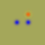
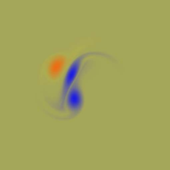
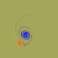
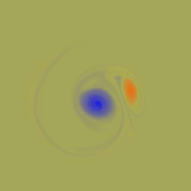
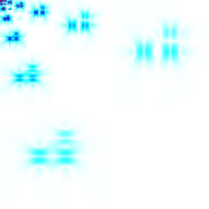
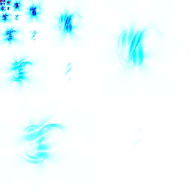
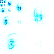
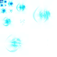
Figure 7: Vorticity fields at times $t=0$, $t=10$, $t=20$ and $t=40$, and corresponding divergence-free wavelet coefficients of the velocity.

The second experiment deals with a decaying two-dimensional turbulent field, obtained with an initial state of random phase spectrum. That vorticity field was computed with the spectral code of [14], at a resolution $1024\times 1024$, and a Reynolds number of $3.5\times 10^{4}$. This field has been kindly provided to us by G. Lapeyre [18]. Figure 8 left represents the vorticity, after $40$ turnover time-scale, where it exhibits the emergence of coherent structures together with strong filamentation of the flow field outside the vortices.
We show in Figure 8 right, the isotropic divergence-free wavelet coefficients of the corresponding velocity field, in $L^{\inf}$-norm.

As expected, the wavelet coefficients get an insight into the energy distribution over the scales of the flow. As one can see on Figure 8, the energy at smallest scale (or highest wavenumbers) is localized along the strong deformation lines, and fits the filamentation between vortices, or with strong changes in vortices. The top-right square corresponding to vertical isotropic wavelets ($\Psi_{\mbox{div},j,\mbox{$\mathbf{k}$}}^{(1,0)}$) exhibits vertical structures, whether the bottom-left square corresponding to horizontal wavelets ($\Psi_{\mbox{div},j,\mbox{$\mathbf{k}$}}^{(0,1)}$) exhibits horizontal deformation lines.

Turbulent vorticity field	Divergence-free wavelet decomposition of the velocity

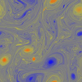
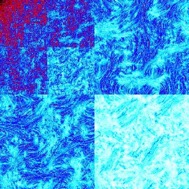
Figure 8: Vorticity field for a $1024\times 1024$ simulation of decaying turbulence (left), and the corresponding divergence-free wavelet coefficients of the velocity field (right).

Now we investigate the compression properties of the divergence-free wavelet analysis: as predicted by the nonlinear approximation theory (see [3]), the compression ratio in energy-norm is governed by the underlying regularity of the velocity field in some Besov space.
Let $\mathbf{u}$ an incompressible field be given, its divergence-free wavelet expansion writes:

$$\mbox{$\mathbf{u}$}=\mbox{$\mathbf{u}$}_{0}+\sum_{j\geq 0}\sum_{\mbox{$\mathbf{k}$}\in\mbox{$\mathbb{Z}$}^{2}}\left(d_{\textrm{div},j,\mbox{$\mathbf{k}$}}^{(1,0)}~{}\Psi_{\textrm{div},j,\mbox{$\mathbf{k}$}}^{(1,0)}+d_{\textrm{div},j,\mbox{$\mathbf{k}$}}^{(0,1)}~{}\Psi_{\textrm{div},j,\mbox{$\mathbf{k}$}}^{(0,1)}+d_{\textrm{div},j,\mbox{$\mathbf{k}$}}^{(1,1)}~{}\Psi_{\textrm{div},j,\mbox{$\mathbf{k}$}}^{(1,1)}\right)$$

The nonlinear approximation of $\mathbf{u}$ relies on computing the best N-terms wavelet approximation by reordering the wavelet coefficients:

$$|d_{\textrm{div},j_{1},\mbox{$\mathbf{k}$}_{1}}^{\varepsilon_{1}}|>|d_{\textrm{div},j_{2},\mbox{$\mathbf{k}$}_{2}}^{\varepsilon_{2}}|>\dots>|d_{\textrm{div},j_{N},\mbox{$\mathbf{k}$}_{N}}^{\varepsilon_{N}}|>\dots$$

and introducing

$$\Sigma_{N}(\mbox{$\mathbf{u}$})=\mbox{$\mathbf{u}$}_{0}+\sum_{i=1}^{N}d_{\textrm{div},j_{i},\mbox{$\mathbf{k}$}_{i}}^{\varepsilon_{i}}~{}\Psi_{\textrm{div},j_{i},\mbox{$\mathbf{k}$}_{i}}^{\varepsilon_{i}}$$ (39)

Then we have

$$\|\mbox{$\mathbf{u}$}-\Sigma_{N}(\mbox{$\mathbf{u}$})\|_{L^{2}}\leq C\left(\frac{1}{N}\right)^{s}\|\mbox{$\mathbf{u}$}\|_{B^{s,q}_{q}}$$ (40)

if the quantity $\|\mbox{$\mathbf{u}$}\|_{B^{s,q}_{q}}^{q}=\sum_{\varepsilon,j,\mbox{$\mathbf{k}$}}\left|d_{\textrm{div},j,\mbox{$\mathbf{k}$}}^{\varepsilon}\right|^{q}$ is finite, with $\frac{1}{q}=\frac{1}{2}+\frac{s}{n}$ (this means that $\mathbf{u}$ belongs to the Besov space $B^{s,q}_{q}$). As stated in [3], the evaluated regularity $s$ can’t be larger than the order of polynomial reproduction in scaling spaces plus one (that equals the number of zero moments of the dual wavelet). In our experiment, the dual spline wavelets $\psi^{*}_{0}$ and $\psi^{*}_{1}$ introduced in 2.2 have respectively two and three zero moments, which only allows us to evaluate regularities smaller than two.
Figure 9 shows the nonlinear compression of divergence-free wavelets, provided on the $1024^{2}$ turbulent field. The curve represents the $L^{2}$-error $\|\mbox{$\mathbf{u}$}-\Sigma_{N}(\mbox{$\mathbf{u}$})\|_{L^{2}}$, versus $N$, in log-log plot. The convergence rate measured on the curve is $s\thickapprox 1.35$ , which induces that the velocity flow belongs to the corresponding Besov space $B^{s,q}_{q}$ with $q=0.85$.
When looking at the compression curve on figure 9, we observe three zones:

- First, large scale wavelets capture the large scale structure of the flows. Consequently, the compression progresses slowly and irregularly.

- Then we observe a linear slope that represents the nonlinear structure of the turbulent flows. In this region, we are able to evaluate the regularity of the field.

- The last region corresponds to an abrupt decrease, due to the fact that the data are discrete.

One can also remark on Figure 9 that only $1.2$% of the coefficients recover about $99$% of the $L^{2}$-norm.

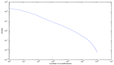
Figure 9: $L^{2}$-error provided by the nonlinear N-best terms wavelet approximation (39): in log-log plot, $L^{2}$-error (40) versus $N$ for a 2D turbulent flow.

The same experiment was carried out on the three interacting vortices, but due to the few number of vanishing moments of the wavelets we use (2), the slope of the curve saturates at $s=2$, meaning that these fields are more regular.

5.3 Analysis of a 3D incompressible field

In this part we consider a three dimensional periodic field, arising from a freely decaying isotropic turbulence, and kindly provided to us by G.-H. Cottet and B. Michaux [4]. The experiment deals with an initial velocity condition of Gaussian distribution, and $128^{3}$ collocation points. Figure 10 displays the vorticity isosurfaces corresponding to about $40\%$ of the maximum vorticity at five turnover times.

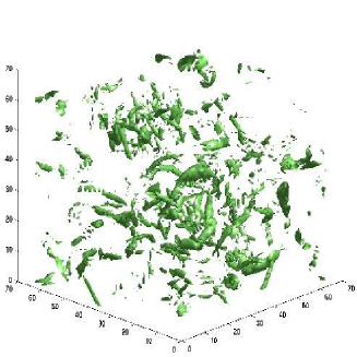
Figure 10: Isosurface of vorticity magnitude after 5 large-eddy turnovers provided by a spectral method [4].

The divergence-free wavelet decomposition of the corresponding velocity field is computed, and displayed on Figures 11 and 12. As explained in section 3.1.2, the isotropic 3D divergence-free wavelet decomposition provides with $14$ generating wavelets $\Psi_{\textrm{div},1,j,\mbox{$\mathbf{k}$}}^{\varepsilon}$, $\Psi_{\textrm{div},2,j,\mbox{$\mathbf{k}$}}^{\varepsilon}$.

Figure 11 left shows the corresponding renormalized coefficients $2^{j}d_{\textrm{div},1,j,\mbox{$\mathbf{k}$}}$, whereas Figure 11 right shows the $2^{j}d_{\textrm{div},2,j,\mbox{$\mathbf{k}$}}$, until $j=6$. The smallest scale ($j=7$) wavelet coefficients are displayed on Figure 12 below, for two kinds of generating wavelets: we choose $\Psi_{\textrm{div},2}^{(1,0,0)}$, which corresponds to horizontal structures, and $\Psi_{\textrm{div},1}^{(0,0,1)}$ which exhibits vertical ones.

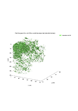
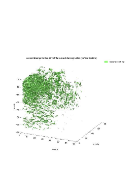
Figure 11: Isosurface $0.2$ of divergence-free wavelet coefficients associated to $\Psi_{\textrm{div},1,j,\mbox{$\mathbf{k}$}}^{\varepsilon}$ (left) and to $\Psi_{\textrm{div},2,j,\mbox{$\mathbf{k}$}}^{\varepsilon}$ (right), in absolute value.

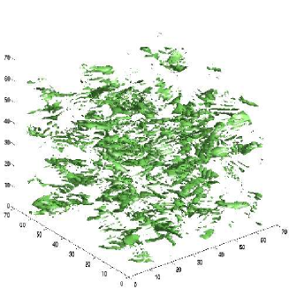
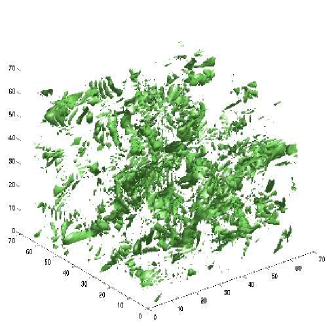
Figure 12: Isosurface $0.06$ of divergence-free wavelet coefficients associated to $\Psi_{\textrm{div},2,J,\mbox{$\mathbf{k}$}}^{(1,0,0)}$ (left) and to $\Psi_{\textrm{div},1,J,\mbox{$\mathbf{k}$}}^{(0,0,1)}$ (right), in absolute value.

Figure 13 displays the nonlinear compression error: we have computed the convergence rate on the linear part of the graph (which is shorter by comparison with the 2D case, due the low resolution) and we have found $s\thickapprox 1.45$.

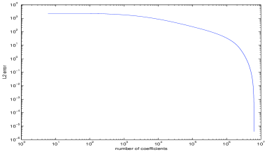
Figure 13: $L^{2}$-error provided by the nonlinear N-best terms wavelet approximation (39): in log-log plot, $L^{2}$-error (40) versus $N$ for a 3D turbulent flow.

5.4 Analysis of 2D compressible fields

We presented in section 4.3, an algorithm which gave rise to a wavelet Hodge decomposition of any flow. In order to numerically prove that it always converges, we have tested the method on various random two-dimensional fields. We constructed some of them by summing random gaussians, and we modified their Fourier spectra in order to vary the regularity. Figure 14 displays the $L^{2}$-norm of the residual, in terms of the number of iterations, for four different vector functions. We can infer the following conclusions:

- For all functions we have tested, the method converges, and curves shows that, except at the early beginning, the convergence is exponential.

- The slope of the curve do not depend to much on the number of grid-points, but the curve itself, corresponding to $1024^{2}$ grid points, is upon these of $256^{2}$ grid points.

- The convergence rate increase with the number of vanishing moments of the dual wavelets.

In the futur, we will investigate the influence of the wavelet bases and of the interpolating projectors, on the convergence rate.

Figure 14: Convergence curves of the iterative wavelet Hodge algorithm.

Since our main objective for further research is to use divergence-free wavelets for solving the Navier-Stokes equations, we have to provide with the wavelet Hodge decomposition of the nonlinear term $(u.\nabla)u$. Indeed, although $\mathbf{u}$ should be incompressible, this term breaks the divergence-free condition and yields a compressible part. As an illustration, we consider as $\mathbf{u}$ the 2D turbulent field displayed on Figure 8, and we compute, by mean of our wavelet Hodge decomposition, the div-free and curl-free wavelet components of $(\mbox{$\mathbf{u}$}.\nabla)\mbox{$\mathbf{u}$}$. Figure 15 shows the anisotropic wavelet coefficients of the divergence-free part (left) and of the curl-free part (right) of the $(\mbox{$\mathbf{u}$}.\nabla)\mbox{$\mathbf{u}$}$ arising from this decomposition.

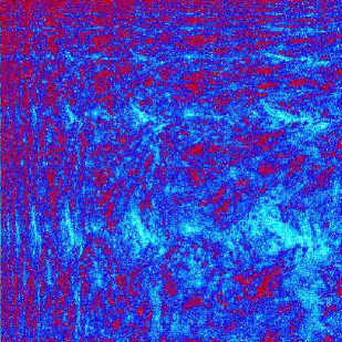
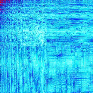
Figure 15: Anisotropic wavelet coefficients corresponding to the wavelet Hodge decomposition of $(\mbox{$\mathbf{u}$}.\nabla)\mbox{$\mathbf{u}$}$: divergence-free coefficients (left), and curl-free coefficients (right).

Figure 16 (left) displays the vorticity field associated to the divergence-free part of $(\mbox{$\mathbf{u}$}.\nabla)\mbox{$\mathbf{u}$}$, while Figure 16 (right) represents the pressure issued from the curl-free term, that is easily reconstructed in wavelet domain, as it will be explain below.

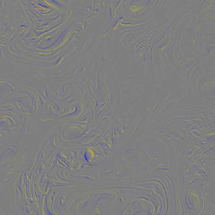
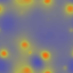
Figure 16: Vorticity (on the left) and pressure (on the right) derived from the wavelet Hodge decomposition of the nonlinear term $\mbox{$\mathbf{u}$}\nabla\mbox{$\mathbf{u}$}$, with $\mathbf{u}$ displayed on Figure 8.

The extracted div-free part of $(\mbox{$\mathbf{u}$}.\nabla)\mbox{$\mathbf{u}$}$ is all what is needed to compute the time-evolution of the velocity in the incompressible Navier-Stokes equations. Thanks to the curl-free wavelet definition, we are also able to directly reconstruct the pressure from the curl-free coefficients of $\nabla p$:
Indeed, with periodic boundary conditions, the curl-free part of $(\mbox{$\mathbf{u}$}.\nabla)\mbox{$\mathbf{u}$}$ writes:

$$[(\mbox{$\mathbf{u}$}.\nabla)\mbox{$\mathbf{u}$}]_{\textrm{curl}~{}1}=\frac{\partial p}{\partial x}= \sum_{j_{1},j_{2}=0}^{J-1}\sum_{k_{1}=0}^{2^{j_{1}}-1}\sum_{k_{2}=0}^{2^{j_{2}}-1}d_{\textrm{curl},k_{1},k_{2}}~{}2^{j_{1}}~{}\psi_{0}(2^{j_{1}}~{}x-k_{1})~{}\psi_{1}(2^{j_{2}}~{}y-k_{2})$$

$$+\sum_{j_{1}=0}^{J-1}\sum_{k_{1}=0}^{2^{j_{1}}-1}d_{\textrm{curl},k_{1}}^{1}~{}2^{j_{1}}~{}\psi_{0}(2^{j_{1}}~{}x-k_{1})$$

$$[(\mbox{$\mathbf{u}$}.\nabla)\mbox{$\mathbf{u}$}]_{\textrm{curl}~{}2}=\frac{\partial p}{\partial y}= \sum_{j_{1},j_{2}=0}^{J-1}\sum_{k_{1}=0}^{2^{j_{1}}-1}\sum_{k_{2}=0}^{2^{j_{2}}-1}d_{\textrm{curl},k_{1},k_{2}}~{}2^{j_{2}}~{}\psi_{1}(2^{j_{1}}~{}x-k_{1})~{}\psi_{0}(2^{j_{2}}~{}y-k_{2})$$

$$+\sum_{j_{2}=0}^{J-1}\sum_{k_{2}=0}^{2^{j_{2}}-1}d_{\textrm{curl},k_{2}}^{2}~{}2^{j_{2}}~{}\psi_{0}(2^{j_{2}}~{}y-k_{2})$$

Be integrating the system (we recall that $\psi_{1}^{\prime}=4~{}\psi_{0}$, see the definition of gradient wavelets), we obtain (up to a constant):

$$4~{}p(x,y)= \sum_{j_{1},j_{2}=0}^{J-1}\sum_{k_{1}=0}^{2^{j_{1}}-1}\sum_{k_{2}=0}^{2^{j_{2}}-1}d_{\textrm{curl},k_{1},k_{2}}\psi_{1}(2^{j_{1}}~{}x-k_{1})~{}\psi_{1}(2^{j_{2}}~{}y-k_{2})$$

$$+\sum_{j_{1}=0}^{J-1}\sum_{k_{1}=0}^{2^{j_{1}}-1}~{}d_{\textrm{curl},k_{1}}^{1}\psi_{1}(2^{j_{1}}~{}x-k_{1})$$

$$+\sum_{j_{2}=0}^{J-1}\sum_{k_{2}=0}^{2^{j_{2}}-1}~{}d_{\textrm{curl},k_{2}}^{2}~{}\psi_{1}(2^{j_{2}}~{}y-k_{2})$$

Thus the computation of the pressure is no more than a standard anisotropic wavelet reconstruction in $V^{1}_{J}\times V^{1}_{J}$, from the curl-free coefficients. By comparison to the pressure computed in Fourier domain, we have found a relative error of $2.5~{}10^{-4}$ in the $L^{2}$-norm, which probably arises from the interpolating process. On the other hand the difference between the Leray projection (in Fourier space) and the wavelet projection onto the divergence-free space represents $1$% of the $L^{2}$-norm, that is to say $0.01$% of the energy. Figure 17 displays the localisation of this error.

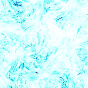
Figure 17: Error between the divergence-free part of $(\mbox{$\mathbf{u}$}.\nabla)\mbox{$\mathbf{u}$}$ (obtained through Fourier transform) and the one provided by the wavelet Hodge decomposition.

Conclusion and perspectives

We have presented in detail the construction of 2D and 3D divergence-free wavelet bases, and a practical way to compute the associated coefficients. We have introduced anisotropic div-free and curl-free wavelet bases, which are more easy to handle. We have shown that these bases make possible an iterative algorithm to compute the wavelet Hodge decomposition of any flow. Thus, numerical tests prove the feasibility of divergence-free wavelets for simulating turbulent flows in two and three dimensions. A divergence-free wavelet based solver for 2D Navier-Stokes equations is underway and will be reported in a forthcoming paper.

An important issue that must be addressed is the great ability of the method: although all numerical tests have been presented in the periodic case, the method extends readily to non-periodic problems, by using wavelets adapted to the proper boundary conditions [28, 24], in the div-free construction. Another point is since we consider the $(\mbox{$\mathbf{u}$},p)$-formulation for the Navier-Stokes equation, and since we are able to compute the Leray projector in the wavelet domain, the method extends easily to the 3D case. At last, this method should be competitive by comparison to a classical Fourier method in the non-periodic case: indeed, the periodic case corresponds to boundary conditions for which spectral methods are obviously fast, while it is clear that wavelet methods take advantage both of the compression properties of the wavelet bases for functions and for operators, in any case.

References

Figure captions

Figure 1: From left to right: the scaling function $\phi$ with its associated symmetric wavelet with shortest support, and their duals: the dual scaling function $\phi^{*}$ and the dual wavelet $\psi^{*}$.

Figure 2: Scaling functions and associated wavelets with shortest support, for splines of degree 1 (left) and 2 (right).

Figure 3: Anisotropic 2D wavelet transform.

Figure 4: Isotropic 2D wavelet transform.

Figure 5: Isotropic 2D generating divergence free wavelets $\Psi_{\textrm{div}}^{(1,0)}$ (left), $\Psi_{\textrm{div}}^{(0,1)}$ (center) and $\Psi_{\textrm{div}}^{(1,1)}$ (right).

Figure 6: The two scaling functions $\phi_{0}$ and $\phi_{1}$, and their symmetry centers.

Figure 7: Vorticity fields at times $t=0$, $t=10$, $t=20$ and $t=40$, and corresponding divergence-free wavelet coefficients of the velocity.

Figure 8: Vorticity field for a $1024\times 1024$ simulation of decaying turbulence (left), and the corresponding divergence-free wavelet coefficients of the velocity field (right).

Figure 9: $L^{2}$-error provided by the nonlinear N-best terms wavelet approximation (39): in log-log plot, $L^{2}$-error (40) versus $N$ for a 2D turbulent flow.

Figure 10: Isosurface of vorticity magnitude after 5 large-eddy turnovers provided by a spectral method [4].

Figure 11: Isosurface $0.2$ of divergence-free wavelet coefficients associated to $\Psi_{\textrm{div},1,j,\mbox{$\mathbf{k}$}}^{\varepsilon}$ (left) and to $\Psi_{\textrm{div},2,j,\mbox{$\mathbf{k}$}}^{\varepsilon}$ (right) in absolute value.

Figure 12: Isosurface $0.06$ of divergence-free wavelet coefficients associated to $\Psi_{\textrm{div},2,J,\mbox{$\mathbf{k}$}}^{(1,0,0)}$ (left) and to $\Psi_{\textrm{div},1,J,\mbox{$\mathbf{k}$}}^{(0,0,1)}$ (right), in absolute value.

Figure 13: $L^{2}$-error provided by the nonlinear N-best terms of wavelet approximation (39): in log-log plot, $L^{2}$-error (40) versus $N$ for a 3D turbulent flow.

Figure 14: Convergence curves of the iterative wavelet Hodge algorithm.

Figure 15: Anisotropic wavelet coefficients corresponding to the wavelet Hodge decomposition of $(\mbox{$\mathbf{u}$}.\nabla)\mbox{$\mathbf{u}$}$: divergence-free coefficients (left), and curl-free coefficients (right).

Figure 16: Vorticity (on the left) and pressure (on the right) derived from the wavelet Hodge decomposition of the nonlinear term $\mbox{$\mathbf{u}$}\nabla\mbox{$\mathbf{u}$}$, with $\mathbf{u}$ displayed on Figure 8.

Figure 17: Error between the divergence-free part of $(\mbox{$\mathbf{u}$}.\nabla)\mbox{$\mathbf{u}$}$ (obtained through Fourier transform) and the one provided by the wavelet Hodge decomposition.

References

- [1] C.-M. Albukrek, K. Urban, W. Dahmen, D. Rempfer, and J.-L. Lumley, Divergence-Free Wavelet Analysis of Turbulent Flows, J. of Scientific Computing 17(1): 49-66, 2002.
- [2] P. Charton, V. Perrier, A pseudo-wavelet scheme for the two-dimensional Navier-Stokes equations, Comp. Appl. Math. 15(2): 139-160, 1996.
- [3] A.Cohen, Wavelet methods in numerical analysis, Handbook of Numerical Analysis, vol. VII, P.G.Ciarlet and J.L.Lions eds., Elsevier, Amsterdam, 2000.
- [4] G.-H. Cottet, B. Michaux, S.Ossia and G. Vanderlinden, A comparison of spectral and vortex methods in three-dimensional incompressible flows, J. Comp. Phys, 175, 2002.
- [5] W. Dahmen, A. Kunoth and K. Urban, A wavelet-Galerkin method for the Stokes problem, Computing 56, 1996, 259-302.
- [6] I. Daubechies, Ten lectures on Wavelets, SIAM book, Philadelphia, Pennsylvania, 1992.
- [7] C. De Boor, A Practical Guide to Splines, book, Springer-Verlag New York Inc., 2001.
- [8] M. Farge, Wavelet transforms and their applications to turbulence, Ann. Rev. Flu. Mech. :395-457, 1992.
- [9] M. Farge, N. Kevlahan, V. Perrier & E. Goirand, Wavelets and turbulence, Proc. IEEE 84(4), 639-669,1996.
- [10] M. Farge and K. Schneider, Coherent Vortex Simulation (CVS), A Semi-Deterministic Turbulence Model Using Wavelets, Flow, Turbulence and Combution, 66: 393-426, 2001.
- [11] J. Fröhlich and K. Schneider, Numerical simulation of decaying turbulence in an adaptive wavelet basis, Appl. Comput. Harmon. Anal., 3: 393-397, 1996.
- [12] V. Girault, P.A. Raviart, Finite element approximations of the Navier-Stokes equations, Lecture Notes in Mathematics, Springer-Verlag, 1979.
- [13] M. Griebel and F. Koster, Adaptive wavelet solvers for the unsteady incompressible Navier-Stokes equations, Advances in Mathematical Fluid Mechanics, J. Malek and J. Necas and M. Rokyta eds, Springer-Verlag, 2000.
- [14] B.L. Hua and D. Haidvogel, Numerical simulations of the vertical structure of quasi-geostrophic turbulence, J. Atmos. Sci. 3:2923-2936, 1986.
- [15] J. Ko, A.J. Kurdila and O.K. Rediniotis, divergence-free Bases and Multiresolution Methods for Reduced-Order Flow Modeling, AIAA Journal, 38(2): 2219-2232, 2000.
- [16] F. Koster and M. Griebel and N. Kevlahan and M. Farge and K. Schneider, Towards an adaptive wavelet-based 3D Navier-Stokes solver, Numerical flow simulation I, Notes on Numerical Fluid Mechanics, Vol. 66, 339-364, E.H. Hirschel eds, Vieweg-Verlag, Braunschweig, 1998.
- [17] J.-P. Kahane and P.-G. Lemarié-Rieusset, Fourier series and wavelets, book, Gordon & Breach, London, 1995.
- [18] G. Lapeyre, Topologie de mélange dans un fluide turbulent géophysique (in french), Thèse de doctorat de l’Université Paris VI, 2000.
- [19] P.-G. Lemarié-Rieusset, Analyses multi-résolutions non orthogonales, commutation entre projecteurs et dérivation et ondelettes vecteurs à divergence nulle (in french), Revista Matemática Iberoamericana, 8(2): 221-236, 1992.
- [20] P.- G. Lemarié-Rieusset, Un théorème d’inexistance pour les ondelettes vecteurs à divergence nulle (in french), C. R. Acad. Sci. Paris, t. 319, Série I, p. 811-813, 1994.
- [21] J. Lewalle, Wavelet transform of the Navier-Stokes equations and the generalized dimensions of turbulence, Appl. Sci. Res. 51(1-2):109-113, 1993.
- [22] S. Mallat, A Wavelet Tour of Signal Processing, book, Academic Press, 1999.
- [23] C. Meneveau, Analysis of turbulence in the orthonormal wavelet representation, Journal of Fluid Mechanics 232: 469-520, 1991.
- [24] P. Monasse and V. Perrier, Orthonormal wavelet bases adapted for partial differential equations with boundary conditions, SIAM J. on Math. Analysis 29(4):1040-1065, 1998.
- [25] K. Schneider, N. Kevlahan, M. Farge, Comparison of an adaptive wavelet method and nonlinearly filtered pseudo-spectral methods for two-dimensional turbulence, Theor. Comput. Fluid Dyn. 9: 191-206, 1997.
- [26] K. Urban, A Wavelet-Galerkin Algorithm for the Driven–Cavity–Stokes–Problem in Two Space Dimensions, RWTH Aachen, Preprint 1994.
- [27] K. Urban, Using divergence free wavelets for the numerical solution of the Stokes problem, AMLI’96: Proceedings of the Conference on Algebraic Multilevel Iteration Methods with Applications, 2: 261–277, University of Nijmegan, The Netherlands, 1996.
- [28] K. Urban, Wavelet Bases in H(div) and H(curl), Mathematics of Computation 70(234): 739-766, 2000.
- [29] K. Urban, Wavelets in Numerical Simulation, Springer, 2002.
- [30]