Abstract

We address here the problem of generating random graphs uniformly from the set of simple connected graphs having a prescribed degree sequence. Our goal is to provide an algorithm designed for practical use both because of its ability to generate very large graphs (efficiency) and because it is easy to implement (simplicity).

We focus on a family of heuristics for which we prove optimality conditions, and show how this optimality can be reached in practice. We then propose a different approach, specifically designed for typical real-world degree distributions, which outperforms the first one. Assuming a conjecture which we state and argue rigorously, we finally obtain an $O(n\log n)$ algorithm, which, in spite of being very simple, improves the best known complexity.

1 Introduction

In the context of large complex networks, the generation of random graphs is intensively used for simulations of various kinds. Until recently, the main model was the Erdös and Renyi [10, 6] one. Many recent studies however gave evidence of the fact that most real-world networks have several properties in common [22, 4, 8, 23] which make them very different from random graphs. Among those, it appeared that the degree distribution of most real-world complex networks is well approximated by a power law, and that this unexpected feature has a crucial impact on many phenomena of interest [7, 23, 22, 11]. Since then, many models have been introduced to capture this feature. In particular, the Molloy and Reed model [20], on which we will focus, generates a random graph with prescribed degree sequence in linear time. However, this model produces graphs that are neither simple nor connected. To bypass this problem, one generally simply removes multiple edges and loops, and then keeps only the largest connected component. Apart from the expected size of this component [21, 3], very little is known about the impact of these removals on the obtained graphs, on their degree distribution and on the simulations processed using them.

The problem we address here is the following: given a degree sequence, we want to generate a random simple connected graph having exactly this degree sequence. Moreover, we want to be able to generate very large such graphs, typically with more than one million vertices, as often needed in simulations.

Although it has been widely investigated, it is still an open problem to directly generate such a random graph, or even to enumerate them in polynomial time, even without the connectivity requirement [24, 18, 19].

In this paper, we will first present the best solution proposed so far [12, 19], discussing both theoretical and practical considerations. We will then deepen the study of this algorithm, which will lead us to an improvement that makes it optimal among its family. Furthermore, we will propose a new approach solving the problem in $O(n\log n)$ time, and being very simple to implement.

2 Context

The Markov chain Monte-Carlo algorithm

Several techniques have been proposed to solve the problem we address. We will focus here on the Markov chain Monte-Carlo algorithm [12], pointed out recently by an extensive study [19] as the most efficient one.

The generation process is composed of three main steps:

1. Realize the sequence: generate a simple graph that matches the degree sequence,

2. Connect this graph, without changing its degrees, and

3. Shuffle the edges to make it random, while keeping it connected and simple.

The Havel-Hakimi algorithm [15, 14] solves the first step in linear time and space. A result of Erdös and Gallai [9] shows that this algorithm succeeds if and only if the degree sequence is realizable.

The second step is achieved by swapping edges to merge separated connected components into a single connected component, following a well-known graph theory algorithm [5, 26]. Its time and space complexities are also linear.

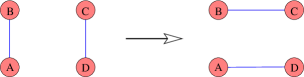
Figure 1: Edge swap

The third step is achieved by randomly swapping edges of the graph, checking at each step that we keep the graph simple and connected. Given the graph $G_{t}$ at some step $t$, we pick two edges at random, and then we swap them as shown in Figure 1, obtaining another graph $G^{\prime}$ with the same degrees. If $G^{\prime}$ is simple and connected, we consider the swap as valid: $G_{t+1}=G^{\prime}$. Otherwise, we reject the swap: $G_{t+1}=G_{t}$

This algorithm is a Markov chain where the space $S$ is the set of all simple connected graphs with the given degree sequence, the initial state $G_{0}$ is the graph obtained by the first two steps, and the transition $G_{t}\to G_{t+1}$ has probability $\frac{1}{m(m-1)}$ if there exists an edge swap that transforms $G_{t}$ in $G_{t+1}$. If there are no such swap, this transition has probability $0$ (note that if $G_{t}=G_{t+1}$, the probability of this transition is given by the number of swaps that disconnect the graph divided by $m(m-1)$).

We will use the following known results:

Theorem 1.

This Markov chain is irreducible [26], symmetric [12], and aperiodic [12].

Corollary 2.

The Markov chain converges to the uniform distribution on every states of its space, i.e. all graphs having the wanted properties.

These results show that, in order to generate a random graph, it is sufficient to do enough transitions. However, no formal result is known about the convergence speed of the Markov chain, i.e. the required number of transitions. A result from Will [28] bounds the diameter of the space $S$ by $m$. Furthermore, massive experiments [12, 19] showed clearly that, even if the original graph (initial state) is extremely biased, $O(m)$ transitions are sufficient to make the graph appear to be “really” random. More precisely, the distributions of a large set of non-trivial metrics (such as the diameter, the flow, and so on) over the sampled graphs is not different from the distributions obtained with random graphs. Notice that we tried, unsuccessfully, to find a metric that would prove this assertion false. Therefore, we will assume the following:

Empirical Result 1.

[19, 12] The Markov chain converges after $O(m)$ swaps.

Equivalence between swaps and transitions

Notice that Empirical Result 1 concerns actual swaps, and not the transitions of the Markov chain: in order to do $O(m)$ swaps one may have to process much more transitions. This point has never been discussed rigorously in the literature, and we will deepen it now. We proved the following result:

Theorem 3.

For any simple connected graph, let us denote by $\rho$ the fraction of all possible pairs of vertices which have distance greater than or equal to $3$. The probability that a random edge swap is valid is at least $\frac{\rho}{2z(z+1)}$, where $z$ is the average degree.

Proof.

If $\rho=0$ the result is trivial. If $\rho>0$, consider a pair $(v,w)$ of vertices having distance $d(v,w)\geq 3$ (i.e. there exist no path of length lower than 3 between $v$ and $w$). Since the graph is connected, there exists a path of length $l\geq 3$  $\left(v,v_{1},\cdots,v_{l-1},w\right)$  connecting $v$ and $w$. The edge swap $(v,v_{1})(w,v_{l-1})\to(v,v_{l-1})(w,v_{1})$ is valid: it does not disconnect the graph, and since the edges it creates could not pre-exist (else we would have $d(v,w)\leq 2$), it keeps it simple.

Now, the $\rho\cdot n(n-1)$ ordered pairs of vertices define at least $\frac{\rho\cdot n(n-1)}{8}$ edges swaps, since an edge swap corresponds to at most $8$ ordered pairs. Therefore, a random edge swap is valid with probability at least $\frac{\rho\cdot n(n-1)}{8m(m-1)}$. The fact that $m=\frac{n\cdot z}{2}$ ends the proof. ∎

In practice, $\rho>0$ (the only connected graphs such that $\rho=0$ are the star-graphs), and its value tends to grow with the size of the graph. Therefore, Theorem 3 makes it possible to deduce from Empirical Result 1 the following result:

Corollary 4 (of Empirical result 1).

The Markov chain converges after $O(m)$ transitions.

Convention 1.

From now on, and in order to simplify the notations, we will take advantage of Theorem 3 and use the terms ”edge swap” and ”transition” indifferently.

Complexity

As we have already seen, the first two steps of the random generation (realization of the degree sequence and connection of the graph) are done in $O(m)$ time and space. The last step requires $O(m)$ transitions to be done (Corollary 4). Each transition consists in an edge swap, a simplicity test, a connectivity test, and possibly the cancellation of the swap (i.e. one more edge swap).

Using hash tables for the adjacency lists, each edge swap and simplicity test can be done in constant time and space. Each connectivity test, on the contrary, needs $O(m)$ time and space. Therefore, the $O(m)$ swaps and simplicity tests are done in $C_{swaps}=O(m)$ time and $O(1)$ space, while the $O(m)$ connectivity tests require $C_{conn}=O(m^{2})$ time and $O(m)$ space. Thus, the total time complexity for the shuffle is quadratic:

$$C_{naive}=O(m^{2})$$ (1)

while the space complexity is linear.

One can however improve significantly this time complexity using the structures described in [16, 17, 27] to maintain connectivity in dynamic graphs. These structures require $O(m)$ space. Each connectivity test can be performed in time $O(\log n/\log\log\log n)$ and each simplicity test in $O(\log n)$ time. Each edge swap then has a cost in $O(\log n(\log\log n)^{3})$ time. Thus, the space complexity is $O(m)$, and the time complexity is given by:

$$C_{dynamic}=O\left(m\log n(\log\log n)^{3}\right)$$ (2)

Notice however that these structures are quite intricate, and that the constants are large for both time and space complexities. The naive algorithm, despite the fact that it runs in $O(m^{2})$ time, is therefore generally used in practice since it has the advantage of being extremely easy to implement. Our contribution in this paper will be to show how it can be significantly improved while keeping it very simple, and that it can even outperform the dynamical algorithm.

Speed-up and the Gkantsidis et al. heuristics

Gkantsidis et al. proposed a simple way to speed-up the shuffle process [12] in the case of the naive implementation in $O(m^{2})$: instead of running a connectivity test for each transition, they do it every $T$ transitions, for an integer $T$ called the speed-up window. Thus, a transition now only consists in an edge swap and a simplicity test, and possibly the cancellation of the swap. If the graph obtained after these $T$ transitions is not connected anymore, the $T$ transitions are cancelled.

They proved that Corollary 2 still holds, i.e. that this process converges to the uniform distribution, although it is no longer composed of a single Markov chain but of a concatenation of Markov chains [12].

The global time complexity of connectivity tests $C_{conn}$ is reduced by a factor $T$, but at the same time the swaps are more likely to get cancelled: with $T$ swaps in a row, the graph has more chances to get disconnected than with a single one. Let us introduce the following quantity:

Definition 1 (Success rate).

The success rate $r(T)$ of the speed-up at a given step is the probability that the graph obtained after $T$ swaps is still connected.

In order to do $O(m)$ swaps, the shuffle process now requires $O(m/r(T))$ transitions, according to Convention 1. The time complexity therefore becomes:

$$C_{Gkan}=O\left(\frac{\displaystyle m+\frac{m^{2}}{T}}{\displaystyle r(T)}\right)$$ (3)

The behavior of the success rate $r(T)$ is not easily predictable. If $T$ is too large, the graph will get disconnected too often, and $r(T)$ will be too small. If on the contrary $T$ is too small, then $r(T)$ will be large but the complexity improvement is reduced. To bypass this problem, Gkantsidis et al. used the following heuristics (see Figure 2).

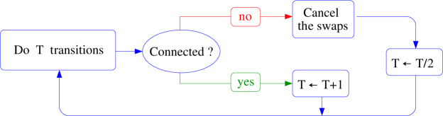
Figure 2: Heuristics 1 (Gkantsidis et al. heuristics)

Heuristics 1 (Gkantsidis et al. heuristics).

IF  the graph got disconnected after $T$ swaps  THEN  $T\leftarrow T/2$  ELSE  $T\leftarrow T+1$

Intuitively, they expect $T$ to converge to a good compromise between a large window $T$ and a sufficient success rate $r(T)$, depending on the graph topology (i.e. on the degree distribution).

3 More from the Gkantsidis et al. heuristics

The problem we address now is to estimate the efficiency of the Gkantsidis heuristics. First, we introduce a framework to evaluate the ideal value for the window $T$. Then, we analyze the behavior of the Gkantsidis et al. heuristics, and get an estimation of the difference between the speed-up factor they obtain and the optimal speed-up factor. We finally propose an improvement of this heuristics which reaches the optimal. We also give experimental evidences for the obtained performance.

The optimal window problem

We introduce the following quantity:

Definition 2 (Disconnection probability).

Given a graph $G$, the disconnection probability $p$ is the probability that the graph gets disconnected after a random edge swap.

Now, let us assume the two following hypothesis:

Hypothesis 1.

The disconnection probability $p$ is constant during  $T$ consecutive swaps

Hypothesis 2.

The probability that a disconnected graph gets reconnected with a random swap, called the reconnection probability, is equal to zero.

Notice that these hypothesis are not true in general. They are however reasonable approximations in our context and will actually be confirmed in the following. We also conduced intensive experiments which gave empirical evidence of this. Moreover, we will give a formal explanation of the second hypothesis in the case of scale-free graphs in Section 4. With these two hypothesis, the success rate $r(T)$, which is the probability that the graph stays connected after $T$ swaps, is given by:

$$r(T)=(1-p)^{T}$$ (4)

Definition 3 (Speed-up factor).

The speed-up factor $\theta(T)$ is the expected number of swaps actually performed between two connectivity tests, which is $0$ if the swaps are cancelled, and $T$ if they are not.

The speed-up factor $\theta(T)$, the success rate $r(T)$ and the disconnection probability $p$ are related as:

$$\theta(T)\ =\ T\cdot r(T)\ =\ T\cdot(1-p)^{T}$$ (5)

The speed-up factor $\theta(T)$ represents the actual gain induced by the speed-up, i.e. the reduction factor of the time complexity of the connectivity tests $C_{conn}$.

Now, given a graph $G$ with disconnection probability $p$, the best window $T$ is the window that maximizes the speed-up factor $\theta(T)$. We find an optimal value $T=1/p$, which corresponds to a success rate $r(T)=1/e$. Finally, we obtain the following theorem:

Theorem 5.

The maximal speed-up factor $\theta_{max}$ is reached if and only if one of the following equivalent conditions is satisfied:

• $T=\frac{1}{p}$

• $r(T)=e^{-1}$

The value of this maximum depends only on $p$ and is given by $\theta_{max}=(p\cdot e)^{-1}$

Analysis of the heuristics

Knowing the optimality condition, we tried to estimate the performance of the Gkantsidis et al. heuristics. Considering $p$ as given, the evolution of the window $T$ under these heuristics leads to :

Theorem 6.

The speed-up factor $\theta_{Gkan}(p)$ obtained with the Gkantsidis heuristics verifies:

$$\forall\epsilon>0,\qquad\theta_{Gkan}=o\left((\theta_{max})^{\frac{1}{2}+\epsilon}\right)\quad when\quad p\to 0$$

Sketch of proof.

We give here a simple mean field approximation leading to the stronger, but approximate result: $\theta_{Gkan}=\Omega\left(\sqrt{\theta_{max}}\right)$. The proof of Theorem 6, not detailled here, follows the same idea.

Given the window $T_{t}$ at step $t$, we obtain an expectation for $T_{t+1}$ depending on the succes rate $r(T_{t})$:

$$\overline{T_{t+1}}=r(T_{t})(T_{t}+1)+(1-r(T_{t}))\frac{T_{t}}{2}$$

We now suppose that $T$ eventually reaches a mean value T. We then obtain:

$$\mathbf{T}=(1-p)^{\mathbf{T}}(\mathbf{T}+1)+\left(1-(1-p)^{\mathbf{T}}\right)\frac{\mathbf{T}}{2}$$

which leads to

$$\frac{\mathbf{T}}{2}=\frac{1}{1-(1-p)^{\mathbf{T}}}-1$$

Therefore, if $p\to 0$ we must have $\mathbf{T}\to\infty$, thus $1-(1-p)^{\mathbf{T}}\to 0$ and finally $1-(1-p)^{\mathbf{T}}\sim p\mathbf{T}$. Therefore:

$$\mathbf{T}\sim\sqrt{\frac{2}{p}}$$

which gives, with Equation 5 and Theorem 5, still for $p\to 0$:

$$\theta_{Gkan}\sim\sqrt{2e\cdot\theta_{max}}$$ (6)

∎

Intuitively, this Theorem means that the Gkantsidis et al. heuristics is too pessimistic: when the graph gets disconnected, the decrease of $T$ is too strong; conversely, when the graph stays connected, $T$ grows too slowly. By doing so, one obtains a very high success rate (very close to 1), which is not the optimal (see Theorem 5).

An optimal dynamics

To improve the Gkantsidis et al. heuristics we propose the following one (with two parameters $q^{-}$ and $q^{+}$) :

Heuristics 2.

IF  the graph got disconnected after $T$ swaps  THEN  $T\leftarrow T\cdot(1-q^{-})$  ELSE  $T\leftarrow T\cdot(1+q^{+})$

The main idea was to avoid the linear increase in $T$, which is too slow, and to allow more flexibility between the two factors $1-q^{-}$ and $1+q^{+}$.

Theorem 7.

With this heuristics, a constant $p$, and for $q^{+},q^{-}$ close enough to $0$, the window $T$ converges to the optimal value and stays arbitrarily close to it with arbitrarily high probability if and only if

$$\frac{q^{+}}{q^{-}}=e-1$$ (7)

Sketch of proof.

If the window $T$ is too large, the success rate $r(T)$ will be small, and $T$ will decrease. Conversely, a too small window $T$ will grow. This, provided that the factors $1+q^{+}$ and $1-q^{-}$ are close enough to $1$, ensures the convergence of $T$ to a mean value T. Like in the proof of Theorem 6, we have:

$$\mathbf{T}=r(\mathbf{T})(1+q^{+})\mathbf{T}+(1-r(\mathbf{T}))(1-q^{-})\mathbf{T}$$

This time, the error made by this approximation can be as small as one wants by taking $q^{+}$ and $q^{-}$ small enough, so that $T$ stays close to its mean value $\mathbf{T}$. It follows that:

$$r(\mathbf{T})=\frac{q^{-}}{q^{+}+q^{-}}$$

This quantity is equal to $e^{-1}$ (optimality condition (ii) of Theorem 5) if and only if $\frac{q^{+}}{q^{-}}=e-1$ ∎

Experimental evaluation of the new heuristics

To evaluate the relevance of these results, based on Hypothesis 1 and 2, and dependent on a constant value of $p$ (which is not the case, since the graph continuously changes during the shuffle) we will now compare empirically the three following heuristics:

1. The Gkantsidis et al. heuristics (Fig. 2, Heuristics 1)

2. Our new heuristics (Heuristics 2)

3. The optimal heuristics: at every step, we compute the window $T$ giving the maximal speed-up factor $\theta_{max}$.

We compared the average speed-up factors obtained with these three heuristics (respectively $\theta_{Gkan}$, $\theta_{new}$ and $\theta_{max}$) for the generation of graphs with various heavy tailed degree sequences. We used a wide set of parameters, and all the results were consistent with our analysis: the average speed-up factor $\theta_{Gkan}$ obtained with the Gkantsidis et al. heuristics behaved asymptotycally like the square root of the optimal, and our average speed-up factor $\theta_{new}$ always reached at least $90\%$ of the optimal $\theta_{max}$. Some typical results on heavy-tailed distributions with $\alpha=2.5$ and $\alpha=3$ are shown below.

$\alpha=2.5$
$z$	$\theta_{Gkan}$	$\theta_{new}$	$\theta_{max}$
2.1	0.79	0.88	0.90
3	3.00	5.00	5.19
6	20.9	112	117
12	341	35800	37000

$\alpha=3$
$z$	$\theta_{Gkan}$	$\theta_{new}$	$\theta_{max}$
2.1	1.03	1.20	1.26
3	5.94	12.3	12.4
6	32.1	216	234
12	578	89800	91000

Table 1: Average speed-up factors for various values of the average degree $z$. We limited ourselves to $n=10^{4}$ because the computations are quite expensive, in particular concerning $\theta_{Gkan}$ and $\theta_{max}$.

These experiments show that our new heuristics is very close to the optimal. Thus, despite the fact that $p$ actually varies during the shuffle, our heuristics react fast enough (in regard to the variations of $p$) to get a good, if not optimal, window $T$. We therefore obtain a success rate $r(T)$ in a close range around $e^{-1}$. From Equation 3 and Theorem 5, we obtain the following complexity for the shuffle:

$$C_{new}=O\left(m+<p>\cdot m^{2}\right)$$ (8)

(where $<p>$ is the average value of $p$ during the shuffle), instead of the $O\left(m+\sqrt{<p>}\cdot m^{2}\right)$ complexity of the Gkantsidis et al. heuristics, also obtained from Eq. 3 and Th. 5. Further empirical comparisons of the two heuristics will be provided in the next section, see Table 2.

Our complexity $C_{new}$, despite the fact that it is asymptotically still outperformed by the complexity of the dynamic connectivity algorithm $C_{dynamic}$ (see Eq. 2), may be smaller in practice if $p$ is small enough. For many graph topologies corresponding to real-world networks, especially graphs having a quite high density (social relations, word co-occurences, WWW), and therefore a low disconnection probability, our algorithm represents an alternative that may behave faster, and which implementation is much easier.

4 A log-linear algorithm ?

We will now show that, in the particular case of heavy-tailed degree distributions like the ones met in practice [11, 22], one may reduce the disconnection probability $p$ at logarithmic cost, thus reducing dramatically the complexity of the connectivity tests. We first outline the main idea, then we present empirical tests showing the asymptotical behavior of the disconnection probability: this leads us to a conjecture, strongly supported by both intuition, experiments and formal arguments, from which we obtain a $O(n\log n)$ algorithm. We finally improve this algorithm, which makes us expect a $O(n\log\log n)$ complexity.

Guiding principle

In a graph with a heavy-tailed degree distribution, most vertices have a very low degree. This means in particular that, swapping two random edges, one has a significant probability to connect two vertices of degree 1 together, creating an isolated component of size 2. One may also create small components of size 3, and so on. Conversely, the non-negligible number of vertex of high degree form a robust core, so that it is very unlikely that a random swap creates two large disjoint components. Therefore, an heavy-tailed distribution implies that when a swap disconnects the graph, it creates in general a small isolated component rather than a large one.

Definition 4 (Isolation test).

An isolation test of width $K$ on vertex $v$ tests wether this vertex belongs to a connected component of size lower than or equal to $K$.

To avoid the disconnection, we now do an isolation test for every transition, just after the simplicity test. If this isolation test returns true, we cancel the swap rightaway. This way, we detect at low cost (as long as $K$ is small) a significant part of the disconnections. As before, we will use Convention 1, considering that every transition corresponds to a valid swap, i.e. a swap that passes both the simplicity and isolation tests.

The disconnection probability $p$ is now the probability that after $T$ swaps which passed the isolation test, the graph gets disconnected. It is straightforward to see that $p$ is decreasing with $K$, even if the relation between them is yet to establish. Therefore, given a graph, the success rate $r$ now depends on both $T$ and $K$.

Empirical study of $p$

Since the disconnection probability $p$ now depends on $K$, and in order to study this relation, we will denote it by $p(K)$ in this subsection. We ran extensive experiments on a very large variety of heavy-tailed degree distributions and graph sizes, as well as real-world network degree distributions. Results are shown in Figure 3 for the degree distribution of the Internet backbone topology presented in [13] (Inet) and for the heavy-tailed degree distribution with the values for $z$ and $\alpha$ that gave the worst results ($g_{2.05}$), i.e. the largest $p(K)$. This worst-case distribution had average degree $z=2.05$ and exponent $\alpha=2.1$.

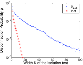
Figure 3: Empirical behavior of $p(K)$ for two degree distributions

We finally state the following conjecture and assume it is true in the sequel:

Conjecture 1.

The average disconnection probability for random simple connected graphs with heavy-tailed degree distributions decreases exponentially with $K$: $p(K)=O(e^{-\lambda K})$ for some positive constant $\lambda$ depending on the distribution, and not on the size of the graph.

The final algorithm

Let us introduce the following quantity:

Definition 5 (Characteristic isolation width).

The characteristic isolation width $K_{G}$ of a graph $G$ having $m$ edges is the minimal isolation test width $K$ such that the disconnection probability $p(K)$ verifies $p(K)<1/m$.

This leads naturally to:

Lemma 8.

Applying the shuffle process to a graph $G$ having at least $10$ edges, with an isolation test width $K\geq K_{G}$, and a period $T$ equal to $m$, we obtain a success rate $r$ larger than $\frac{1}{3}$.

Proof.

Even without Hypothesis 2, the success rate is always greater than or equal to $(1-p)^{T}$. Choosing $K\geq K_{G}$ and $T=m$, we obtain:

$$r\geq\left(1-\frac{1}{m}\right)^{m}$$

which is larger than $\frac{1}{3}$ for $m\geq 10$ ∎

Moreover, still assuming Conjecture 1, and because $m=O(n)$ for the degree distributions we consider:

Lemma 9.

For a given degree distribution, the characteristic isolation width $K_{G}$ of random graphs of size $n$ is in $O(\log n)$

It follows that:

Theorem 10.

For a given degree distribution, the shuffle process for graphs of size $n$ has complexity $O(n\log n)$ time and $O(m)$ space.

Proof.

Let us define the procedure shuffle(G) as follows:

1. set $K$ to $1$,

2. save the graph $G$,

3. do $m$ edge swaps on $G$ with isolation tests of width $K$,

4. if the obtained graph is connected, then return it,

5. else, restore $G$ to its saved value, set $K$ to $2\cdot K$, and go back to step 2.

This procedure returns a connected graph obtained after applying $m$ edge swaps to $G$. Lemma 8 and 9 ensure that this procedure ends after $O(\log\log n)$ iterations with high probability. Moreover, the cost of iteration $i$ is $O(2^{i}\cdot m)$, since dominating complexity comes from the $O(m)$ isolation tests of width $2^{i}$. Therefore, we obtain a global complexity of $O(m\log n)$ time. We have $m=O(n)$, so that the complexity is finally $O(n\log n)$ time. The space complexity is straightforward. ∎

One can easily check that the heuristics presented in Figure 4 is at least as efficient as the one presented in this proof. It aims at equilibrating $C_{swaps}$ and $C_{conn}$ by dynamically adjusting the isolation test width $K$ and the window $T$, keeping a high success rate $r(K,T)$ and a large window $T$ (here we impose $T\geq\frac{m}{10}$).

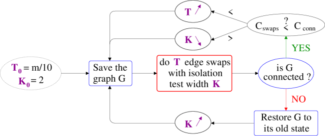
Figure 4: Our final heuristics used to adjust the isolation test width $K$ and the window $T$ in an implementation of the log-linear algorithm.

We compare in Table 2 typical running times obtained for various sizes and for an heavy-tailed degree distribution with the naive algorithm, the Gkantsidis et al. heuristics, our improved version of this heuristics, and our final algorithm. Notice that our final algorithm allows to generate massive graphs in a very reasonable time, while the previously used heuristics could need several weeks to do so. The limitation for the generation of massive graphs now comes from the memory needed to store the graph more than the computation time. Implementations are provided at [29].

$m$	Naive	Gkan. heur.	Heuristics 2	Final algo.
$10^{3}$	0.51s	0.02s	0.02s	0.02s
$10^{4}$	26.9s	1.15s	0.47s	0.08s
$10^{5}$	3200s	142s	48s	1.1s
$10^{6}$	$\approx$ 4$\cdot 10^{5}$s	$\approx$ 3$\cdot 10^{4}$s	10600s	25.9s
$10^{7}$	$\approx$ 4$\cdot 10^{7}$s	$\approx$ 3$\cdot 10^{6}$s	$\approx$ $10^{6}$s	420s

Table 2: Average computation time for the generation of graphs of various sizes with an heavy-tailed degree distribution of exponent $\alpha=2.5$ and average degree $z=6.7$ (on a Intel Centrino 1.5MHz with 512MB RAM).

Towards a $O(n\log\log n)$ algorithm ?

The isolation tests are typically breadth- or depth-first searches that stop when they have visited $K+1$ vertices. Taking advantage of the heavy-tailed degree distribution, we may be able to reduce their complexity as follows: if the search meets a vertex of degree greater than $K$, it can stop because it means that the component is large enough. This is a first improvement.

Moreover, if the search is processed in an appropriate way, like a depth-first search directed at the neighbour of highest degree, it may reach a vertex of degree greater than $K$ in only a few steps. Several recent results indicate that searching a vertex of degree at least $K$ in an heavy-tailed network takes $O(\log K)$ steps in average [25, 2, 1]. Thus, running an isolation test after an edge swap that did not disconnect the graph would be done in $O(\log\log n)$ time instead of $O(\log n)$.

In the case of a swap that disconnected the graph, we also have the following result:

Lemma 11.

For a given heavy-tailed degree distribution, the expected complexity of an isolation test, knowing that it returned true, is constant.

Proof.

Knowing that the test returned true, the probability $s_{i}$ that the isolated component had a size equal to $i$ is given by:

$$s_{i}=\frac{p(i)-p(i+1)}{p(0)-p(K+1)}$$

where $p(k)$ is the disconnection probability for an isolation test width $k$. Using Conjecture 1 that assumes an exponential decrease of $p(k)$, it follows that the expectation of the size of this isolated component is $O(1)$. ∎

Finally, the complexity of any isolation test would be $O(\log\log n)$ time, so that the global complexity would become $O(n\log\log n)$ time.

5 Conclusion

Focusing on the speed-up method introduced by Gkantsidis et al. for the Markov chain Monte Carlo algorithm, we introduced a formal background allowing us to show that this heuristics is not optimal in its own family. We improved it in order to reach the optimal, and empirically confirmed the results.

Going further, we then took advantage of the characteristics of real-world networks to introduce an original method allowing the generation of random simple connected graphs with heavy-tailed degree distributions in $O(n\log n)$ time and $O(m)$ space. It outperforms the previous best known methods, and has the advantage of being extremly easy to implement. We also have pointed directions for further enhancements to reach a complexity of $O(n\log\log n)$ time. The empirical measurement of the performances of our methods show that it yields significant progress. We provide an implementation of this last algorithm [29].

Notice however that the last results rely on a conjecture, for which we gave several arguments and strong empirical evidences, but were unable to prove.

Appendix A Evaluation of the bias of the common method

The “common method” to generate random simple connected graphs with a prescribed degree sequence is the following :

1. Generate a graph $G$ with the Molloy and Reed model [20].

2. Remove the multiple edges and loops, obtaining a simple graph $G_{S}$.

3. Keep only the largest connected component, obtaining a simple connected subgraph $G_{CS}$

In the following, we also call $G_{C}$ the subgraph obtained by step 3 without step 2 ($G_{C}$ is the non-simple giant connected component of $G$). It is clear that $G_{S}$, $G_{C}$ and $G_{CS}$ are different from $G$. We provide here experimental evidences that this difference is significant. Since our model doesn’t suffer of any such bias, as it is simple and connected from the beginning, we recommend its use for anyone who needs to generate random simple connected graphs with a prescribed degree sequence.

Notations

We call $N$ the number of vertices in $G$, $M$ the number of edges and $Z$ the average degree. Likewise, $N_{C}$, $N_{S}$, $N_{CS}$, $M_{C}$, $M_{S}$, $M_{CS}$, $Z_{C}$, $Z_{S}$ and $Z_{CS}$ refer respectively to $G_{C}$, $G_{S}$ and $G_{CS}$.

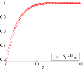
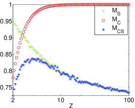
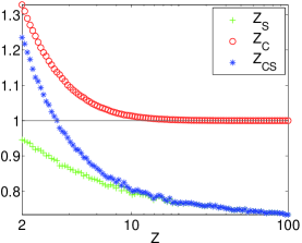
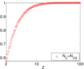
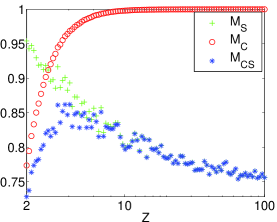
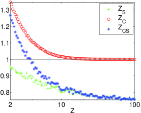
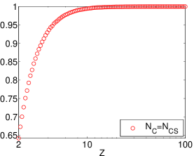
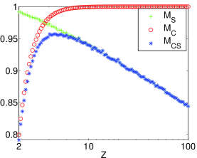
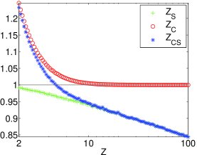
Figure 5: Comparison of the number of vertices (left), the number of edges (center) and the average degree (right) in the graphs $G_{S}$, $G_{C}$ and $G_{CS}$, for various values of the average degree $Z$ of the original graph $G$. We used heavy-tailed degree distributions with $N=10^{4},\alpha=2.1$ (top), $N=10^{5},\alpha=2.1$ (middle) and $N=10^{4},\alpha=2.5$ (bottom).

Plots

To quantify the modifications caused by the removal of multiple edges and/or the restriction to the giant connected component, we plotted the number of vertices, the number of edges and the average degrees of the concerned subgraphs $G_{C}$, $G_{S}$ and $G_{CS}$ against the average degree of $G$. In each plot, the three curves refer to $G_{C}$ (red circles), $G_{S}$ (green plus) and $G_{CS}$(blue stars). The quantities are normalized so that a value of $1$ represents the value of the concerned quantity in $G$.

Notice that, since $N_{S}$ is always equal to $N$ (the removal of edges by itself does not change the number of vertices), we only plotted $N_{C}$, which is also equal to $N_{CS}$.

Discussion

Many things can be observed from those plots. In particular :

• The left and middle plots show clearly that one loses a significant part of the graph when performing multiple edge removal, restricting to the giant component, or both.

• The similarity between the plots at the top and in the middle show that the size $N$ has very little, if any, influence on this loss. The only noticeable difference comes fom the fact that the top plots, due to their lower computation costs, were averaged on more instances than the middle ones.

• The bottom plots are closer to $1$, meaning that the bias is less significant. This is due to the greater exponent $\alpha$, causing the heavy-tailed degree distribution to be less heterogenous. Thus, less vertices have very low degree (these ones get more likely removed in $G_{C}$) or very high degree (these ones are more likely to get many edges removed in $G_{S}$).

• The left part of the plots (low average degree $Z$) show a significant loss of vertices in $G_{C}$. This is of course because the more edges we have, the bigger the giant connected component is. On the other hand, the right part of the plots (high average degree $Z$) show an increasing loss of edges due to the removal of more multiple edges.

• The plots on the right-hand side show that two opposite biases act on the average degree $Z_{CS}$ of $G_{CS}$: the multiple edges removals tends to lower it, while the removal of vertices that don’t belong to the giant component tends to raise it (since these vertices more likely have a low degree).

Conclusions

We showed that the bias caused by the two last steps of the “common method” is significant, not only on the size of the graph but also on its properties, like the average degree. These biases should therefore cause the deviation of many other properties. Our model, which respect exactly the degree sequence given at the beginning, represents a reference that may be used to better quantify these deviations. Its simplicity and efficiency should also convince users to implement it (or to use our implementation, available at [29]). Notably, it provides an easy way to separate the properties of the known models, like the Barabàsi-Albert one, in two groups: the ones that come from the degree distribution only, and the ones that come from the model itself.

References

- [1] L. A. Adamic, R. M. Lukose, and B. A. Huberman. Local search in unstructured networks. In Handbook of Graphs and Networks: From the Genome to the Internet, pages 295–317. Wiley-VCH Verlag, 2003.
- [2] L. A. Adamic, R. M. Lukose, A. R. Puniyani, and B. A. Huberman. Search in power-law networks. Phys. Rev. E, 64(046135), 2001.
- [3] W. Aiello, F. Chung, and L. Lu. A random graph model for massive graphs. Proc. of the 32nd ACM STOC, pages 171–180, 2000.
- [4] R. Albert and A. Barabási. Statistical mechanics of complex networks. Reviews of Modern Physics, 74:47, 2002.
- [5] C. Berge. Graphs and Hypergraphs. North-Holland, 1973.
- [6] B. Bollobas. Random Graphs. Academic Press, London - New York, 1985.
- [7] A. Clauset and C. Moore. Traceroute sampling makes random graphs appear to have power law degree distributions. cond-mat/0312674, 2003.
- [8] S.N. Dorogovtsev and J.F.F. Mendes. Evolution of networks. Adv. Phys., 51:1079, 2002.
- [9] P. Erdos and T. Gallai. Graphs with prescribed degree of vertices. Mat. Lapok, 11:264–274, 1960.
- [10] P. Erdös and A. Rényi. On random graphs. Publ. Math. Debrecen, 6:290–291, 1959.
- [11] M. Faloutsos, P. Faloutsos, and C. Faloutsos. On power-law relationships of the internet topology. Proc. ACM SIGCOMM, 29:251–262, 1999.
- [12] C. Gkantsidis, M. Mihail, and E. Zegura. The markov chain simulation method for generating connected power law random graphs. Proc. of ALENEX’03, LNCS, pages 16–25, 2003.
- [13] R. Govindan and H. Tangmunarunkit. Heuristics for internet map discovery. Proc. of IEEE INFOCOM’00, pages 1371–1380, 2000.
- [14] S. L. Hakimi. On the realizability of a set of integers as degrees of the vertices of a linear graph. SIAM Journal, 10(3):496–506, 1962.
- [15] V. Havel. A remark on the existence of finite graphs. Caposis Pest. Mat., 80:496–506, 1955.
- [16] M. R. Henzinger and V. King. Randomized fully dynamic graph algorithms with polylogarithmic time per operation. Journal of the ACM, 46(4):502–516, 1999.
- [17] J. Holm, K. de Lichtenberg, and M. Thorup. Poly-logarithmic deterministic fully-dynamic algorithms for connectivity, minimum spanning tree, -edge, and biconnectivity. Proc. of the 30th ACM STOC, pages 79–89, 1998.
- [18] J. M. Roberts Jr. Simple methods for simulating sociomatrices with given marginal totals. Social Networks, 22:273–283, 2000.
- [19] R. Milo, N. Kashtan, S. Itzkovitz, M. E. J. Newman, and U. Alon. Uniform generation of random graphs with arbitrary degree sequences. submitted to Phys. Rev. E, 2001.
- [20] M. Molloy and B. Reed. A critical point for random graphs with a given degree sequence. Random Structures and Algorithms, pages 161–179, 1995.
- [21] M. Molloy and B. Reed. The size of the giant component of a random graph with a given degree sequence. Combinatorics, Probability and Computing, 7:295, 1998.
- [22] M. E. J. Newman. The structure and function of complex networks. SIAM Review, 45(2):167–256, 2003.
- [23] M. E. J. Newman, S. H. Strogatz, and D. J. Watts. Random graphs with arbitrary degree distributions and their applications. Phys. Rev. E, 64(026118), 2001.
- [24] A. R. Rao, R. Jana, and S. Bandyopadhyay. A markov chain monte carlo method for generating random (0,1)-matrices with given marginals. Indian Journal of Statistics, 58(A):225–242, 1996.
- [25] N. Sarshar, P. O. Boykin, and R. Roychowdhury. Scalable percolation search in power law networks. Proc. of 4th IEEE conference on Peer-to-peer networks (P2P’04), pages 2–9, 2004.
- [26] R. Taylor. Constrained switchings in graphs. Combinatorial Mathematics, 8:314–336, 1980.
- [27] Mikkel Thorup. Near-optimal fully-dynamic graph connectivity. Proc. of the 32nd ACM STOC, pages 343–350, 2000.
- [28] T. G. Will. Switching distance between graphs with the same degrees. SIAM Journal on Discrete Mat., 12(3):298–306, 1999.
- [29] www.liafa.jussieu.fr/fabien/generation.